


 Abstract
 HTML
HTML Reference
 Related
 PDF
PDF


-
Two-body non-leptonic B meson decays play an essential role in particle physics to help us understand quantum chromodynamics (QCD) and CP violation in the standard model (SM) [1–4]. With precision measurements, such decays also provide a window to investigate possible new physics beyond the SM [5–8].
Since the Large Hadron Collider began operation at CERN, the LHCb Collaboration has provided a number of more precise B decay measurements than the B factories. The High Luminosity phase of the Large Hadron Collider will improve the measurement of B decay channels with the integrated luminosity increasing from
$ 23 \, {\rm{fb^{-1}}} $ in Phase 1 to$ 300 \, {\rm{fb^{-1}}} $ in Phase 2 [3]. After the successful operation of the B factory, an upgrade of Super-KEKB is expected to provide 50 times more data [4], which will provide another independent precise measurement. Belle-II is expected to improve the measurement of most charmless two-body B decays. For example, the measurement of direct CP violation in the$B \to K^\ast \pi, K \rho, \, K^\ast \rho$ channels could be improved greatly to achieve the same accuracy as that of$ K\pi $ channels. Another type of precision measurement in Belle-II focuses on decays to two vector meson final states. Besides the branching ratios, more physical observables in these decays, such as the perpendicular polarization fraction ($ f_\perp $ ), relative phase ($ \varphi_\parallel, \, \varphi_\perp, \, \delta_0 $ ), and helicity CP asymmetry parameters ($ {{\cal{A}}}_{CP}^0, \, {{\cal{A}}}_{CP}^\perp $ ), are awaiting measurement.On the theoretical side, high precision calculation of two-body charmless B decays is moving forward on a variety of fronts within different approaches. One example is the light cone sum rules (LCSRs) approach, which is a traditional method of calculating heavy-to-light transition form factors [9–15]. Form factors are key inputs for many factorization approaches on hadronic B decays. The high order power corrections in this method have been performed in recent years. A systematic power correction study on the radiative leptonic decay
$ B \to \gamma l \nu_l $ [16, 17] shed light on sub-leading twist B meson wave function information [18], which includes key inputs for the study of hadronic B meson decay. Besides the form factors, the LCSRs approach is also applied to two-body non-leptonic$ B \to \pi\pi $ decays [19–22].The QCD calculation of non-leptonic B decays has a long history. The first attempt was the naive factorization approach [23, 24], which assumed that the two body non-leptonic decay amplitude is a production of transition form factors and the meson decay constant. The so called generalized factorization approach was the first to include the perturbative QCD (PQCD) corrections of effective operators and the chiral enhanced penguin contribution in hadronic B decays [25, 26]. The factorization is approved order by order later in the QCD factorization approach (QCDF) [27, 28], allowing the calculation of high order QCD corrections and leaving the non-perturbative parameters to be determined by experiments [29]. The vertex corrections to the tree amplitudes [30, 31] and penguin amplitudes [32, 33] were recently obtained at next-to-next-to-leading-order (NNLO). These calculations, together with the next-to-leading-order (NLO) calculations of spectator scattering (NNLO in
$ \alpha_s $ ) [34–36], compose the full corrections to the hard kernels at NNLO. By introducing different fields in different energy regions, an improved factorization approach known as soft-collinear effective theory (SCET) is established by two-step matching [37–40]. SCET has simple kinematics but complicated dynamics with several typical scales, which results in a more apparent and efficient factorization formalism.Although the NNLO calculation has been performed in the QCDF, the dominant contribution for hadronic B decays originates from transition form factors, which are not calculable in the QCDF. In the QCDF/SCET, the transverse momentum of the valence quark is often neglected to simplify the perturbative calculation; however, this results in endpoint divergence in the Feynman diagram of form factor calculation. This divergence also occurs in annihilation type diagrams, which is not a physical divergence. Recently, leading order (LO) weak annihilation diagrams were shown to be calculable without encountering end-point divergence by considering the hard-collinear gluon exchange effect [41]. In the PQCD factorization approach [42, 43], the transverse momenta
$ k_T $ are collected for each external light quark line to regularize the end-point singularity. The additional scale$ k_T $ will result in extra logarithms in the QCD calculation, which may spoil the perturbative expansion. Resummation techniques are performed for large logarithms, resulting in a Sudakov exponent, which highly suppresses the dynamics in small$ k_T $ and small x, where x is the longitudinal momentum fraction of partons in a meson. Two-body charmless B decays were first calculated at LO with the PQCD approach for$ PP $ , with P denoting a pseudo-scalar meson [44–46],$ PV $ [47, 48], with V denoting a vector meson, and$ VV $ [49–51] final states, which provided a correct prediction of the first direct CP asymmetry measurement in B decays. A recent global analysis of all$ B\to PP $ ,$ PV $ decays in the LO PQCD approach is also available [52].With the success of the LO PQCD results and increasingly precise experimental measurements, NLO corrections in PQCD are required to improve the accuracy of the approach. There are two types of NLO corrections to two-body charmless B decays in the framework of
$ k_T $ factorization: the first is associated with the four fermion effective operators, and the second is accompanied by the transition matrix elements sandwiched between a B meson and two light mesons. The first type includes vertex correction, quark loop correction, and chromo-magnetic penguin correction to the operator$ O_{8g} $ . These corrections are first considered in PQCD to investigate$ B \to \pi K, \phi K $ puzzles [53, 54]. One part of these NLO correlations is included in the effective Wilson coefficients, whereas the other parts provide the independent decay amplitudes for certain channels. The second type of NLO QCD corrections carries the dynamics from the$ m_B $ scale to the hadronic scale, which are manifested by means of heavy-to-light transition form factors [55, 56], the timelike form factors of final light mesons [57–61], Glauber effects in the hard scattering spectator and annihilation amplitudes [62–64], and other possible corrections that have not been studied in detail [65]. Besides the QCD correction at NLO, the sub-leading power corrections from high twist light cone distribution amplitudes (LCDAs) were recently studied for pion form factors and the radiative leptonic decay$ B \to \gamma l \nu_l $ in the PQCD approach [66–68].The effects of the NLO corrections mentioned above have been partly examined case by case in several charmless two-body B decay channels [69–78]. The theoretical precision was explicitly improved with a lower theoretical uncertainty, and the agreement between PQCD predictions and experimental measurements were effectively improved for the branching ratios and other physical observables. In this review, we summarize all 78 channels of charmless
$ B \to PP, PV, VV $ decays in the PQCD approach using updated input parameters. With the inclusion of all currently known NLO QCD and power corrections, we discuss some longstanding "puzzle" channels, particularly for$B \to K \pi, K\rho, K^\ast \pi, K^\ast\rho$ decays.This paper is organized as follows. In the next section, the three scale factorization approach is introduced in terms of the effective Hamilton of b quark decay and the definition of meson wave functions. In Section III, we exhibit the PQCD calculation of charmless hadronic B decay matrix elements at LO. We then discuss the NLO corrections in Section IV. The phenomenological results for all two-body charmless decays,
$ B \to PP $ ,$ PV $ , and$ VV $ , are discussed in Section V. The summary is given in the final section. -
All charmless B meson decays are weak decays in the SM and are induced by charged current. Because the W boson mass is significantly larger than the b quark mass, the heavy W boson and top quark are typically integrated out to obtain the effective Hamiltonian of four quark operators with QCD corrections. The relevant effective Hamiltonian of
$ b \to q U \bar{U} $ decays with$ U \in \{ u, c\} $ and$ q \in \{ d, s \} $ is$ \begin{aligned}[b] {{\cal{H}}}_{{\rm{eff}}}(\Delta b = - 1) =& \frac{{G_\rm{F}}}{\sqrt{2}} \Big[ V_{U q}^\ast \, V_{Ub} \left( C_1(\mu) \, O_1(\mu) + C_2(\mu) \, O_2(\mu) \right) \\ & - V_{tq}^\ast \, V_{tb} \, \sum_{i=3}^{10} \, C_{i}(\mu) \, O_{i}(\mu) \\&- V_{tq}^\ast \, V_{tb} C_{8g}(\mu) \, O_{8g}(\mu) \Big] , \end{aligned} $

(1) where
$ V_{ij} $ are the CKM matrix elements. With the chiral representation of the fermion fields$ \left(\bar{q}_1 q_2\right)_{{\rm{V-A}}} = \bar{q}_1 \gamma_\mu (1 - \gamma_5) q_2 $ and$ \left(\bar{q}_1 q_2\right)_{{\rm{V+A}}} = \bar{q}_1 \gamma^\mu (1 + \gamma_5) q_2 $ , the local operators involved in nonleptonic B decay processes are$ \begin{aligned}[b] O_1 =& \left( \bar{q}_\alpha \, U_\beta \right)_{{\rm{V-A}}} \left( \bar{U}_\beta \, b_\alpha \right)_{{\rm{V-A}}} \,,\\ O_2 =& \left( \bar{q}_\alpha \, U_\alpha \right)_{{\rm{V-A}}} \left( \bar{U}_\beta \, b_\beta \right)_{{\rm{V-A}}} \,, \end{aligned} $

(2) $ \begin{aligned}[b]O_3 =& \left( \bar{q}_\alpha \, b_\alpha \right)_{{\rm{V-A}}} \sum_{q^\prime} \left( \bar{q}^\prime_\beta \, q^\prime_\beta \right)_{{\rm{V-A}}} \,, \\ O_4 =& \left( \bar{q}_\alpha \, b_\beta \right)_{{\rm{V-A}}} \sum_{q^\prime} \left( \bar{q}^\prime_\beta \, q^\prime_\alpha \right)_{{\rm{V-A}}} \,, \\ O_5 =& \left( \bar{q}_\alpha \, b_\alpha \right)_{{\rm{V-A}}} \sum_{q^\prime} \left( \bar{q}^\prime_\beta \, q^\prime_\beta \right)_{{\rm{V+A}}} \,, \\ O_6 =&\left( \bar{q}_\alpha \, b_\beta \right)_{{\rm{V-A}}} \sum_{q^\prime} \left( \bar{q}^\prime_\beta \, q^\prime_\alpha \right)_{{\rm{V+A}}} \,, \end{aligned} $

(3) $ \begin{aligned}[b] O_7 = &\frac{3}{2} \left( \bar{q}_\alpha \, b_\alpha \right)_{{\rm{V-A}}} \sum_{q^\prime} e_{q^\prime} \left( \bar{q}^\prime_\beta \, q^\prime_\beta \right)_{{\rm{V+A}}} \,, \\ O_8 =& \frac{3}{2} \left( \bar{q}_\alpha \, b_\beta \right)_{{\rm{V-A}}} \sum_{q^\prime} e_{q^\prime} \left( \bar{q}^\prime_\beta \, q^\prime_\alpha \right)_{{\rm{V+A}}} \,, \\O_9 =& \frac{3}{2} \left( \bar{q}_\alpha \, b_\alpha \right)_{{\rm{V-A}}} \sum_{q^\prime} e_{q^\prime} \left( \bar{q}^\prime_\beta \, q^\prime_\beta \right)_{{\rm{V-A}}} \,, \\ O_{10} = &\frac{3}{2} \left( \bar{q}_\alpha \, b_\beta \right)_{{\rm{V-A}}} \sum_{q^\prime} e_{q^\prime} \left( \bar{q}^\prime_\beta \, q^\prime_\alpha \right)_{{\rm{V-A}}} \,, \end{aligned} $

(4) $ O_{8 g} = \frac{g_s}{8 \pi^2} \, m_b \, \bar{q}_\alpha \, \sigma^{\mu\nu} \left( 1 + \gamma_5 \right) T_{\alpha\beta}^a \, G_{\mu\nu}^a \, b_\beta \,. $

(5) These effective operators are grouped into current-current (tree) operators,
$ O_{1,2} $ , QCD (electroweak) penguin operators,$ O_{3-6} $ ($ O_{7-10} $ ), and the chromomagnetic operator$ O_{8 g} $ .The Wilson coefficients
$ C_{1-10} $ and$ C_{8g} $ are obtained by matching the effective Hamiltonian with the full theory of weak decays [79–82], including the NLO QCD corrections. The explicit renormalization scale dependence of the Wilson coefficients should be canceled by the matrix elements of the effective operators. For this reason, in the LO calculation of the PQCD factorization approach, we usually use LO Wilson coefficients, although NLO corrections are already on the market [45]. -
Because the masses of charmless mesons are all negligible compared with the large B meson mass, the two final state mesons are in the collinear state with large momenta in the rest frame of the B meson. It is convenient to work in light cone coordinates. If we define one of the outgoing light meson directions as "-," its momentum in the light cone coordinates is
$ \begin{eqnarray} p_3 = \frac{1}{\sqrt{2}} \left( 0, m_B, {\bf{0}}_T \right) . \end{eqnarray} $

(6) The valence quark (anti-quark) in this final state meson is also collinear and its momentum is
$ x_3p_3 $ ($ \bar x_3p_3=(1-x_3)p_3 $ ). Here,$ x_3 $ is the momentum fraction carried by the quark, as defined in the parton model. All charmless two body B decays are characterized by b quark weak decay through the four quark operators defined in Eqs. (2)–(4). The large b quark mass ensures that all three final state light quarks from the four-quark operator are energetic (collinear); hence, a hard gluon is required to kick the spectator quark, which is soft in the B meson, to make it collinear and therefore form the final light mesons.The hard gluon connects the spectator quark to the four quark operators, producing the four Feynman diagrams for nonleptonic two-body B decays in the framework of the PQCD approach at LO, which is depicted in Fig. 1(a)–(d). Fig. 1(a) and (b) are also the leading Feynman diagrams in the QCDF and SCET framework in numerical calculations. The main difference between these approaches is the treatment of Fig. 1(a) and (b). For example, in the calculation of the second diagram, the gluon propagator along with the quark propagator are proportional to
$ x_1^2x_2 $ , which appears in the denominator of the decay amplitude. The range of a parton momentum fraction x is not experimentally controllable and spans from 0 to 1. Hence, the endpoint region with$ x \to 0 $ is unavoidable. The leading twist distribution amplitude is proportional to x; therefore, the leading diagram in Fig. 1(a) and (b) diverges in the endpoint region. In QCDF, researchers argue that these two diagrams can be treated as the generalized factorization approach and are products of transition form factors and the meson decay constant. As a result, the most important diagrams in the numerical calculation of the QCDF are not perturbatively calculable.
Figure 1. (color online) Leading order Feynman diagrams of two-body hadronic
$ \bar{B}^0/B^- $ decays. The two black dots denote the vertices of the effective four quark operator.In fact, at the endpoint region, when
$ x\to 0 $ , the transverse momentum of the valence quark is no longer negligible. In the PQCD approach, we keep the transverse momentum of quarks at the denominator of the decay amplitude to remove endpoint divergence [44, 45]. However, in the numerator of the decay amplitude, we still neglect the transverse momentum compared with the large longitudinal momentum. After this treatment, the gauge invariance of the decay amplitude is maintained, and the endpoint singularity is avoided. The introduction of transverse momentum enriches the study of hadron distribution amplitudes, where the light-cone aligned definition is corrected to the transverse momentum dependent definition with a general Wilson link. The collinear factorization breaks down, and$ k_T $ factorization should be adopted. It has been shown that infrared divergences appearing in loop corrections to exclusive processes can be absorbed into hadron LCDAs in$ k_T $ factorization without breaking the gauge invariance [83]. The transverse momentum of a quark is an extra scale in the QCD calculation of the decay amplitude, which results in extra logarithms to spoil the perturbative expansion. These double logarithms should be resummed using the renormalization group equation to repair the perturbative expansion. The resummation is performed to the leading logarithms or next-to-leading logarithms to produce a$ k_T $ Sudakov factor [84], which exhibits high suppression for large distances (small$ k_T $ when$ x \sim 0 $ ). Integrating over the transverse momentum, the decay amplitude is still proportional to the logarithm term$ \ln^2 x $ . To improve the perturbative expansion in the PQCD approach, these logarithms are also resummed by the so called threshold resummation [85–88]. Remarkably, the two-stage application of resummation repairs the self-consistency between the perturbative strong coupling$ \alpha_s(t) $ and the hard logarithm$ \ln (x_1x_2Q/t^2) $ . Here, t is the factorization scale, which is typically chosen at the largest virtuality in hard scattering, that is, the characterized factorization scale in the$ B \to \pi l \nu $ decay is$ t \sim 8 \Lambda_{\rm QCD} m_b $ . The typical infrared divergence, including the soft divergence and collinear divergence, in the PQCD approach is treated the same way as those in soft-collinear effective theory [37], which we do not discuss in detail.There is also the possibility that the light quark of the B meson is one of the quarks in the four quark operators, with a light quark anti-quark pair generated by a hard gluon. These types of Feynman diagrams are usually called annihilation type diagrams, which are shown in Fig. 1(e)–(h). Because the B meson is a pseudoscalar meson, its decay into two massless quarks in a weak interaction is helicity suppressed. These diagrams are neglected in the generalized factorization approach [25]. Similar to Fig. 1(a) and (b), an endpoint singularity also exists in the calculation of annihilation type diagrams. Their contributions in the QCDF are parametrized as free parameters to be fitted from experiments. Again, we can perform the PQCD calculation of these diagrams in PQCD by including the transverse momentum of valence quarks in the meson.
For the topological emission diagrams in Fig. 1(a) and (b), the decaying amplitudes are real functions because this transition occurs in the space-like region, whereas in the annihilation topology, the decaying amplitudes are complex functions with internal propagators varying in the shell, which can be re-expressed using the identity
$ \begin{eqnarray} \frac{1}{k_T^2 - xm_B^2 - {\rm i} \epsilon} = {{\cal{P}}} \left( \frac{1}{k_T^2 - xm_B^2} \right) + {\rm i} \pi \delta(k_T^2 - xm_B^2). \end{eqnarray} $

(7) Here,
$ {{\cal{P}}} (f) $ is the Cauchy principal value obtained by evenly approaching the singular point from both sides such that the diverging pieces cancel each other out. This is not in conflict with the hard mechanism of the amplitudes, which implies a large off-shellness. In fact, on-shell configuration indeed occurs for internal propagators, even though the soft mechanism is highly suppressed by the Sudakov exponents, that is, the factorizable annihilation amplitudes in the$ B \to \pi\pi $ decay are proportional to the timelike pion form factor, where the energy dependent imaginary part continues from the resonance region to the$ {{\cal{O}}}(m_B^2) $ energy region. The strong phase in Eq. (7) may induce large$ {C P} $ violation in two-body hadronic B meson decays, which is essential to explain the large direct CP asymmetry of$ B^0\to K^+\pi^- $ [44] and$ B^0\to \pi^+\pi^- $ [45] decays.Besides the annihilation amplitudes, there are other sources of strong phase in the PQCD approach. The first candidate is the Sudakov exponent, which is related to the center of mass scattering angle and the angular distribution of scattering hadrons. This contribution may be important in baryon decays owing to the angle distribution, whereas in the B meson decays, it is negligible. The second candidate originates from the NLO corrections to the spectator emission amplitudes with the Glauber gluon [62–64]. This effect only supplies a sizable phase to the pion final state and modifies the interactions between different topological amplitudes. The strong phase from the quark loop correction, with an on shell charm quark, is the leading strong phase in the QCDF but a type of NLO correction in
$ \alpha_s $ expansion. Note that all these sources of strong phases reflect either the soft or Glauber gluon corrections to the wave function at high orders, whereas the on shell configuration of the annihilation amplitudes is mechanized by the hard gluon exchange at LO.The ultraviolet divergence in high order calculations is investigated using the standard renormalization method, which we do not discuss in detail. The large ultraviolet logarithms
$ \ln (m_W/t) $ and$ \ln (t/\Lambda_{{\rm{QCD}}}) $ are summed using the standard renormalization-group method to give two-stage evolutions, where the interaction that occurs in the energy interval$ t \sim {{\cal{O}}} [m_b, m_W] $ is described by the effective Wilson coefficients, and the interaction that occurs below the energy scale t is demonstrated by the hadronic transition matrix element. The renormalization scale dependences cancel in these two evolutions, which results in a scale independent amplitude, producing a reliable prediction for charmed B decays [89–91]. The standard formula of the PQCD approach used to handle an exclusive scattering/weak decay is expressed by a combination of the hard scattering mechanism and transverse momentum dependent wave functions, with the guidance of the factorization theorem to detach the physical amplitude according to the acting intervals between interactions.By employing the resummation techniques to sum all the double and single logarithms between the W boson mass, b quark mass, and transverse momentum, the three scale factorization schemes allow us to calculate the two-body B decays perturbatively. The decay amplitude can therefore be expressed in the convolution of hard kernels and meson LCDAs.
$ \begin{aligned}[b] {{\cal{M}}}(B \to M_2M_3) =& H_{r}(M_W, t ) \otimes H(t,\mu) \otimes \phi(x,P^+,b,\mu) \\ =& \sum_{i} C_i(M_W,t) \otimes H_i(t,b) \otimes \phi(x,b,1/b) \\& \cdot \exp \Bigg[ -s(P^+,b) - \int_{1/b}^{t} \frac{{\rm d}\overline{\mu}}{\overline{\mu}} \gamma_\phi(\alpha_s(\overline{\mu}))\Bigg]. \end{aligned} $

(8) Here,
$ H_r $ ($ C_i $ ) is the hard kernel (Wilson coefficients) carrying the first-stage evolution stretched from$ m_W $ down to the t scale,$ H(t,\mu) $ is the perturbative calculable hard part shown in Fig. 1,$ H_i \otimes \phi $ is taken along the second-stage evolution from the hard scale t down to$\Lambda_{\rm QCD}$ , in which ϕ is the LCDAs defined with a certain twist in the meson wave functions.$ s(P^+,b) $ in the exponent is the so called Sudakov factor resulting from the resummation of double logarithms, and$ \gamma_\phi $ is the anomalous dimension of the wave function emerging from the resummation of the single logarithms in quark self-energy correction. -
B meson distribution amplitude is defined under heavy quark effective theory by dynamical twist expansion [92–96]. The leading LCDA of a B meson in momentum space is
$ \begin{aligned}[b] &\int {\rm d}^4z_1 \, {\rm e}^{{\rm i} \bar{k}_1 \cdot z_1} \big\langle 0 \vert \bar{d}_\sigma(z_1) \, b_{ \beta}(0) \vert \bar{B}^0(p_1) \big\rangle \\ =& \frac{{\rm i} f_B}{\sqrt {2 N_c}} \Bigg\{ ( \not p_1 + m_B) \gamma_5 \Bigg[ \frac{ \not n_+}{\sqrt{2}} \varphi_+(\bar{x}_1, b_1) \\&+ \left( \frac{ \not n_-}{\sqrt{2}} - k_1^+ \gamma_\perp^\nu \frac{\partial}{\partial {\bf{k}}^\nu_{1 T}}\right) \varphi_-(\bar{x}_1, b_1) \Bigg] \Bigg\}_{\beta\sigma} \, \\ =& \frac{-{\rm i} }{\sqrt {2 N_c}} \left\{ ( \not p_1 + m_B) \gamma_5 \left[ \varphi_B(x_1, b_1) - \frac{ \not n_+ - \not n_-}{\sqrt{2}} \bar{\varphi}_B(x_1, b_1) \right] \right\} _{\beta\sigma} \,. \end{aligned} $

(9) Here,
$ x_1 = k_1^-/p_1^- $ denotes the momentum fraction of an antiquark moving along the minus direction on the light cone; the underlying integral$\varphi_{\pm} (x_1, b_1)= $ $ \int {\rm d} k_1^+ {\rm d}^2 {\boldsymbol k}_{\rm{1T}} {\rm e}^{{\rm i} {\boldsymbol k}_{\rm{1T}} \cdot {\boldsymbol b}_1} \times \varphi_{\pm}(k_1)$ is implemented. To obtain the approximate expression in the 2nd line, we omit the transverse projection term. The following comments are made to explain the definition:$ (1) $ The definition of matrix elements in Eq. (9) is only valid in factorizable scatterings in which the hard interaction occurs locally, independent of nonlocal matrix elements.$ (2) $ By definition, it is easy to show that$ \begin{aligned}[b] \varphi_B(x_1, b_1) =& \frac{1}{2} \left[ \varphi_+(x_1, b_1) + \varphi_-(x_1, b_1) \right] \,, \\ \bar{\varphi}_B(x_1, b_2) =& \frac{1}{2} \left[ \varphi_-(x_1, b_1) - \varphi_+(x_1, b_1) \right] \,. \end{aligned} $

(10) The contribution from the LCDA
$ \bar{\varphi}_B(x_1) = \bar{\varphi}_B(x_1, 0) $ is argued to be suppressed by$ {\cal{O}}(\ln \frac{\bar{\Lambda}}{m_B}) $ , in contrast with$ \varphi_B(x_1) $ [97], by the relation$\varphi_-(x) = \int_x^\infty {\rm d} x' \, \varphi_+(x')/x'$ and the hadronic scale$ \bar{\Lambda} \simeq m_B - m_b $ . In the symmetry limit of$ \varphi_+ $ and$ \varphi_- $ , we have$ \varphi_B = \varphi_+ $ and$ \bar{\varphi}_B = 0 $ . This approximation is employed in our calculation with an accuracy of up to$ {\cal{O}}(\bar{\Lambda}/m_b) $ . We note that broken symmetry between$ \varphi_+ $ and$ \varphi_- $ has been considered recently in two-body hadronic B decays, and the result is positive for the approximation [98].$ (3) $ The LCDA is usually parameterized in the exponential model,$ \begin{eqnarray} \varphi_B(x_1,b_1) = N_B \,x_1^2 \, (1-x_1)^2 \, {\rm{exp}} \left[ - \frac{x_1^2m_B^2}{2 \omega_B^2} - \frac{(\omega_B b_1)^2}{2} \right] , \end{eqnarray} $

(11) where the parameter
$ N_B $ is determined by the distribution amplitude normalization as$ \begin{eqnarray} \int_0^1 {\rm d} x_1 \, \varphi_B(x_1, b_1=0) = \frac{f_B}{2 \sqrt{2N_c}} \,. \end{eqnarray} $

(12) -
LCDAs are rigorously defined by the matrix element sandwiched by quark bilinears with light-cone separation and then switch to actual momenta and a lightlike distance x for the practice of phenomena.
In this paper, we do not consider the three-particle LCDAs of light mesons, whose contributions can be expected to be power suppressed in B decays, although three-particle LCDAs relate to high twist LCDAs with two-particle assignment via the equation of motion [99]. The three-particle LCDA contributions are carefully examined in the π and K electromagnetic and transition form factor [66, 68] and are at least one order of magnitude smaller than the two-particle contribution in the large energy region
$ Q^2 \geqslant 10 \, {\rm{GeV}}^2 $ . In momentum space, the vacuum to pion matrix element with possible currents can be expressed in the twist expansion in the following form up to twist-3 accuracy:$ \begin{aligned}[b] & \int {\rm d}^4z \, {\rm e}^{-{\rm i} \bar{k} \cdot z} \,\big\langle \pi^+(p) \big\vert \bar{u}_\delta(0) \, d_\alpha(z) \big\vert 0 \big\rangle \\ =& \frac{-\rm i }{\sqrt {2N_c}} \, \Big\{ \gamma_5 \Big[ \, \not p \, \varphi_\pi^{\rm{a}}( x, b) + m_0^\pi \, \varphi_\pi^{\rm{p}}(x, b) \\&-m_0^\pi \left( \not n_+ \not n_- - 1\right) \, \varphi_\pi^{\rm{t}}(x, b) \Big] \Big\}_{\alpha\delta} . \end{aligned} $

(13) $ f_\pi $ is the decay constant,$ m_0^\pi \equiv m_\pi^2/(m_u+m_d) $ is the chiral mass, and$ \varphi_\pi^a $ and$ \varphi^{{\rm{p}}, \sigma}_\pi $ are the LCDAs at dynamical leading twist and twist-3, respectively. They both have the normalization$\int_0^1 {\rm d} x \, \varphi_\pi^{\rm{a}}(x) = f_{\pi}/2\sqrt{2N_c}$ .LCDAs are usually formulated using conformal partial expansion and expressed in terms of the Gegenbauer polynomials
$ C_n^{j/2} $ . The leading twist LCDA of pseudoscalar mesons is$ \begin{eqnarray} \varphi_P^{\rm{a}}(x, \mu) = \frac{f_{\pi}}{2\sqrt{2N_c}}6x\bar{x} \sum_{n=0} \, a^P_n(\mu) \, C_n^{3/2}(2x-1) \,. \end{eqnarray} $

(14) Two-particle twist-3 LCDAs are related to the three-particle LCDA and leading twist LCDA by the QCD equation of motion. The parameter
$ \rho^P = (m_{q_1}+m_{q_2})/m_0^P $ is then introduced to reflect the quark mass terms in the equation of motion. Up to the accuracy, with conformal spin at NLO and the second Gegenbauer moment, the LCDAs of pseudoscalar mesons are$ \begin{aligned}[b] \varphi^{\rm{p}}_P(x, \mu) =& \frac{f_{\pi}}{2\sqrt{2N_c}} \Bigg[1 + 3 \rho^P \Big( 1-3a_1^P+6a_2^P\Big)(1+\ln x) \\&- \frac{\rho^P}{2} \Big( 3-27a_1^P+54a_2^P\Big) \, C_1^{1/2}(2x-1) \\ &+ 3 \Big(10 \eta_{3P} - \rho^P (a_1^P - 5 a_2^P) \Big) \, C_2^{1/2}(2x-1) \\&+ \Big(10 \eta_{3P} \lambda_{3P} - \frac{9}{2}\rho^Pa_2^P \Big) \, C_3^{1/2}(2x-1) \\ &- 3 \eta_{3P} \omega_{3P} \, C_4^{1/2}(2x-1) \Bigg] \, , \end{aligned} $

(15) $ \begin{aligned}[b] \varphi_P^{\rm{t}}(x, \mu)=& \frac{1}{6} \, \frac{\rm d}{{\rm d} x }\varphi_P^\sigma(x, \mu), \\ \varphi_P^\sigma(x, \mu) =& \frac{f_{\pi}}{2\sqrt{2N_c}} 6x(1-x) \Bigg\{ 1 + \frac{\rho^P}{2} \Big(2 - 15 a_1^P + 30 a_2^P\Big) \\&+ \rho^P \Big(3a_1^P - \frac{15}{2}a_2^P\Big) \, C_1^{3/2}(2x-1) \\ &+ \frac{1}{2} \Big( \eta_{3P}(10-\omega_{3P}) + 3\rho^P a_2^P \Big) \, C_2^{3/2}(2x-1) \\&+ \eta_{3P} \lambda_{3P} \, C_3^{3/2}(2x-1) \\ &+ 3 \rho^P \Big( 1- 3a_1^P + 6 a_2^P \Big) \, \ln x \Bigg\} \,. \end{aligned} $

(16) In the above expression, contributions from the three-particle and two-particle configurations by the equation of motion are clearly separated. The three-particle parameters
$ f_{3P} $ ,$ \lambda_{3P} $ , and$ \omega_{3P} $ are defined by the matrix element of local twist-3 operators, and their evolutions have mixing terms with the quark mass [100]. In our case, we only consider the mass of the strange quark, neglecting the$ u, d $ quark masses. Furthermore, we do not include the terms proportional to the parameters$ f_{3P}, \lambda_{3P}, \omega_{3P} $ within the present accuracy. -
The longitudinal and transverse decay constants of vector mesons are defined as
$ \begin{aligned}[b] \big\langle \rho^+(p, \epsilon^\lambda) \big\vert \bar{u}(0) \gamma_\tau d(0) \big\vert 0 \big\rangle =& - {\rm i} f^\parallel_\rho m_\rho \epsilon^\lambda_\tau \,, \\ \big\langle \rho^+(p, \epsilon^\lambda) \big\vert \bar{u}(0) \sigma_{\tau,\tau^\prime} d(0) \big\vert 0 \big\rangle =& - {\rm i} f^\perp_\rho \left( \epsilon^\lambda_\tau p_{\tau^\prime} - \epsilon^\lambda_{\tau^\prime} p_\tau \right) \,. \end{aligned} $

(17) In the convenient momentum space used in practice, the matrix elements of vacuum to vector mesons up to twist-3 are arranged for longitudinal and transverse polarization, respectively,
$ \begin{aligned}[b] &\int {\rm d}^4 z \, {\rm e}^{-{\rm i} \bar{k} \cdot z} \, \big\langle \rho^+(p, \epsilon^\parallel) \big\vert \bar{u}_{\delta}(0) d_\alpha(z) \big\vert 0 \big\rangle \\ =&\frac{-{\rm i} }{\sqrt {2N_c}} \left\{m_\rho \not \epsilon \,^\parallel \, \varphi_{\rho}^\parallel( x) + \not \epsilon \,^\parallel \not p \, \varphi_{\rho}^{t,\parallel}( x) - m_\rho \, \bar{\psi}_{\rho}^{s,\parallel}( x) \right\}_{\alpha\delta} \,, \end{aligned} $

(18) $ \begin{aligned}[b] &\int {\rm d}^4z \, {\rm e}^{-{\rm i} \bar{k} \cdot z} \, \big\langle \rho^+(p, \epsilon^\perp) \big\vert \bar{u}_{\delta}(0) d_\alpha(z) \big\vert 0 \big\rangle \\ =&\frac{-{\rm i} }{\sqrt {2N_c}} \Bigg\{ \not \epsilon \,^\perp \not p \, \varphi_{\rho}^\perp( x) + m_\rho \not \epsilon\,^\perp\, \varphi_{\rho}^{t,\perp}( x) \\&- \frac{{\rm i} \, m_\rho}{(p \cdot n_-)} \varepsilon_{\tau\tau'\kappa\kappa'} \gamma_5 \gamma^\tau \epsilon^{\perp \tau'} p^\kappa n_-^{\kappa'} \, \bar{\psi}_{\rho}^{s,\perp}(x) \Bigg\}_{\alpha\delta} \,. \end{aligned} $

(19) The normalizations of the LCDAs
$ \varphi_\rho = \{ \varphi^{\parallel(\perp)}_\rho, \varphi_{\rho}^{t,\parallel(\perp)} \} $ are$ \begin{aligned}[b] \int_0^1 {\rm d} x \, \varphi^{\parallel(\perp)}_\rho(x) =&\frac{f^{\parallel(\perp)}_{\rho}}{2\sqrt{2N_c}} \,,\\ \int_0^1 {\rm d} x \, \varphi_{\rho}^{t,\parallel(\perp)}(x) =& \frac{1}{2\sqrt{2N_c}} \left(f^{\perp(\parallel)}_{\rho} - f^{\parallel(\perp)}_{\rho} \frac{m_u+m_d}{m_\rho} \right)\,. \end{aligned} $

(20) The LCDAs of light vector mesons are more complicated than those of pseudoscalars owing to the polarizations, which are quoted as [99, 101, 102]
$ \varphi^\parallel_{V}(x, \mu) =\frac{3 f_\rho^\parallel}{\sqrt{6}} x\bar{x} \sum_{n=0} \, a^{V, \parallel}_n(\mu) \, C_n^{3/2}(2x-1) \,, $

(21) $ \begin{aligned}[b] \varphi^{t,\parallel}_{V}(x, \mu) =& \frac{3 f_\rho^\perp}{2\sqrt{6}} (2x-1) \Big\{C_1^{1/2}(2x-1) \\&+ \, a_{V, 1}^\perp \, C_2^{1/2}(2x-1) + \, a_{V, 2}^\perp \, C_3^{1/2}(2x-1) \Big\} \,, \end{aligned} $

(22) $ \begin{eqnarray} \psi^{s,\parallel}_{V}(x, \mu) = \frac{3 f_\rho^\perp}{2\sqrt{6}} x\bar{x} \left\{1 + \frac{a_{V,1}^\perp}{3} \, C_1^{3/2}(2x - 1) + \frac{a_{V, 2}^\perp}{6} \, C_2^{3/2}(2x - 1) \right\} \,. \end{eqnarray} $

(23) $ \begin{eqnarray} \varphi^\perp_{V}(x, \mu) &=& \frac {3 f_\rho^\perp}{\sqrt{6}} x\bar{x} \sum_{n=0} \, a^{V, \perp}_n(\mu) \, C_n^{3/2}(2x-1) \,, \end{eqnarray} $

(24) $ \begin{aligned}[b] \varphi^{t,\perp}_{V}(x, \mu) =& \frac{3 f_\rho^\parallel}{8 \sqrt{6}} \big\{ [1 + (2x-1)^2] + 2\, a_{V,1}^{\parallel} \, (2x-1)^3\\& +8 \, a_{V, 2}^\parallel \, C_2^{1/2}(2x-1) + \frac{6}{7} \, a_{V, 2}^\parallel \, C_4^{1/2}(2x-1) \big\} \,, \end{aligned} $

(25) $ \begin{aligned}[b] \psi^{s,\perp}_{V}(x, \mu) =& \frac{3 f_\rho^\parallel}{4 \sqrt{6}} x\bar{x} \Bigg\{1 + \frac{a_{V,1}^\parallel}{3} \, C_1^{3/2}(2x-1) \\&+ \frac{a_{V, 2}^\parallel}{6} \, C_2^{3/2}(2x-1) \Bigg\} \,. \end{aligned} $

(26) Note the relation
${\bar \psi}^{s,\perp(\parallel)}_{V}(x) = \dfrac{\rm d}{{\rm d}x} \psi^{s,\perp(\parallel)}_{V}(x)$ . For isospin-half light mesons (K and$ K^\ast $ ), the definition of LCDAs is similar to that of isospin-vector mesons (π and ρ) if substituting non-perturbative parameters, such as$ m_{K^{(\ast)}}, f_{K^{(\ast)}}, m_0^{K^{(\ast)}}, a_n^{K^{(\ast)}}, \rho^{K^{(\ast)}} $ . -
For the isospin-singlet light mesons η and
$ \eta^\prime $ , mixing [103–105] should be considered. We consider the$ \eta_q-\eta_s $ mixing scheme [106, 107], where the physical states are expressed as a linear combination of the orthogonal quark-flavor basis$ \eta_q = (\bar{u}u + \bar{d}d)/\sqrt{2} $ and$ \eta_s = \bar{s}s $ via the octet-singlet basis$ \eta_1 = (\bar{u}u + \bar{d}d + \bar{s}s)/\sqrt{3} $ and$ \eta_8 = (\bar{u}u + \bar{d}d - 2\bar{s}s)/\sqrt{6} $ via$ \begin{aligned}[b] \left( \begin{array}{c} \big\vert \eta \rangle \\ \big\vert \eta^\prime \rangle \end{array} \right) =& U(\theta) \, \left( \begin{array}{c} \big\vert \eta_8 \rangle \\ \big\vert \eta_1 \rangle \end{array} \right) \, = U(\phi) \, \left( \begin{array}{c} \big\vert \eta_q \rangle \\ \big\vert \eta_s \rangle \end{array} \right) \,\\ =& \left( \begin{array}{ccc} \cos \phi & - \sin \phi \\ \sin \phi & \cos \phi \end{array} \right) \, \left( \begin{array}{c} \big\vert \eta_q \rangle \\ \big\vert \eta_s \rangle \end{array} \right) \, . \end{aligned} $

(27) The decay constants of physical states,
$ \begin{aligned}[b] \big\langle 0 \big\vert \, \bar{q} \gamma_\tau \gamma_5 q \, \big\vert \eta (\eta') \big\rangle =& {\rm i} f_{\eta (\eta')}^{q} p_\tau \,, \\\big\langle 0 \big\vert \, \bar{s} \gamma_\tau \gamma_5 s \, \big\vert \eta (\eta') \big\rangle =& {\rm i} f_{\eta (\eta')}^{s} p_\tau \,, \end{aligned} $

(28) are obtained from those of the quark flavor basis,
$ \begin{eqnarray} &&\big\langle 0 \big\vert \, \bar{q} \gamma_\tau \gamma_5 q \, \big\vert \eta_q (p) \big\rangle = \frac{\rm i}{\sqrt{2}} \, p_\tau \, f_q \,, \,\,\,\,\,\, \big\langle 0 \big\vert \, \bar{s} \gamma_\tau \gamma_5 s\, \big\vert \eta_s (p) \big\rangle = {\rm i} \, p_\tau \, f_s \, \end{eqnarray} $

(29) by the same rotation, which are written in terms of mass independent superpositions of
$ f_q $ and$ f_s $ $ \begin{eqnarray} \left( \begin{array}{c c } f_\eta^q & f_\eta^s \\ f_{\eta^\prime}^q & f_{\eta^\prime}^s \end{array} \right) = U(\phi) \, \left( \begin{array}{c c} f_q & 0 \\ 0 & f_s \end{array} \right) \,. \end{eqnarray} $

(30) Considering the well-known anomaly of axial vector currents,
$ \begin{aligned}[b] \partial^\tau \left(J_{\tau, 5}^{q} \right) =& \sqrt{2} \left( m_u \bar{u} \gamma_5 u + m_d \bar{d} \gamma_5 d + \frac{\alpha_s}{4\pi} G \tilde{G} \right) \,, \\ \partial^\tau \left(J_{\tau, 5}^{s} \right) =& 2 m_s \bar{s} \gamma_5 s + \frac{\alpha_s}{4\pi} G \tilde{G} \,, \end{aligned} $

(31) where
$ J_{\tau, 5}^{q} = \dfrac{1}{\sqrt{2}} (\bar{u} \gamma_\tau \gamma_5 u + \bar{d} \gamma_\tau \gamma_5 d) $ ,$ J_{\tau, 5}^{s} = \bar{s} \gamma_\tau \gamma_5 s $ ,$ m_i $ is the current quark mass, and G and$ \tilde{G} $ are the gluon field strength tensor and its dual, respectively. Similar to those defined in Eq. (28), the matrix elements of the axial vector current are given by the product of the decay constants of mesons and the square of meson mass as follows:$ \begin{aligned}[b] &\left\langle 0 \left\vert \partial^\tau \left( \begin{array}{c c}J_{\tau, 5}^{q} & 0 \\ 0 & J_{\tau, 5}^{s}\end{array} \right)\right\vert \left(\begin{array}{c c} \eta & 0 \\ 0 & \eta^\prime \end{array} \right) \right\rangle \\=& \left(\begin{array}{c c } m_{\eta}^2 & 0 \\ 0 & m_{\eta^\prime}^2 \end{array} \right) \left(\begin{array}{c c } f_\eta^q & f_\eta^s \\ f_{\eta^\prime}^q & f_{\eta^\prime}^s \end{array} \right) = {\cal{M}}^2 U(\phi) \left( \begin{array}{c c} f_q & 0 \\ 0 & f_s \end{array} \right) \,, \end{aligned} $

(32) which resolves the mass matrix in the quark flavor basis,
$ \begin{aligned}[b] {\cal{M}}_{qs}^2 =& U^\dagger(\phi) {\cal{M}}^2 U(\phi) \\=& \left( \begin{array}{c c} m_{qq}^2+\dfrac{\sqrt{2}}{f_q}\big\langle 0 \big\vert \dfrac{\alpha_s}{4\pi} G \tilde{G} \big\vert \eta_q \big\rangle & \dfrac{1}{f_s}\big\langle 0 \big\vert \dfrac{\alpha_s}{4\pi} G \tilde{G} \big\vert \eta_q \big\rangle \\ \dfrac{\sqrt{2}}{f_q}\big\langle 0 \big\vert \dfrac{\alpha_s}{4\pi} G \tilde{G} \big\vert \eta_s \big\rangle & m_{ss}^2+\dfrac{1}{f_s}\big\langle 0 \big\vert \dfrac{\alpha_s}{4\pi} G \tilde{G} \big\vert \eta_s \big\rangle \end{array} \right) \, \end{aligned} $

(33) with the quark mass contributions
$ \begin{aligned}[b] m_{qq}^2 \equiv& {\rm i} \frac{\sqrt{2}}{f_q} \big\langle 0 \big\vert m_u \bar{u} \gamma_5 u + m_d \bar{d} \gamma_5 d \big\vert \eta_q \big\rangle \\ =& m_\eta^2 \cos^2 \phi + m^2_{\eta^\prime} \sin^2\phi- \frac{\sqrt{2}f_s}{f_q} \left( m^2_{\eta^\prime} - m^2_\eta \right) \cos\phi \sin\phi \,, \\ m_{ss}^2 \equiv& \frac{2}{f_s} \big\langle 0 \big\vert m_s \bar{s} \gamma_5 s \big\vert \eta_s \big\rangle = m_\eta^2 \sin^2 \phi + m^2_{\eta^\prime} \cos^2\phi \\&- \frac{f_q}{\sqrt{2}f_s} \left( m^2_{\eta^\prime} - m^2_\eta \right) \cos\phi \sin\phi\,. \end{aligned} $

(34) The chiral mass entered into the high twist LCDAs of the quark flavour
$ \eta_{i} $ state is$ m_0^i \equiv m_{ii}^2/(2 m_i) $ , with$ i=q,s $ . The$ \eta_q $ and$ \eta_s $ components of$ \eta, \eta^\prime $ mesons obey a similar twist expansion to that in pion and kaon mesons. -
The main uncertainty in the PQCD approach arises from higher order QCD corrections and the nonperturbative parameters of meson LCDAs. The high order QCD corrections characterized by the variation in the factorization scale are usually minimized by setting the factorization scale as the largest virtuality in hard scattering processes. We adopt a two-loop expression for the strong coupling constant with the
$ \beta_{1,2} $ functions [108]$ \begin{eqnarray} \alpha_s(\mu) = \frac{\pi}{2\,\beta_1\, {\rm{log}}(\mu/\Lambda^{(n_f)})} \left[ 1 - \frac{\beta_2}{\beta_1^2} \, \frac{ {\rm{log}}(2\, {\rm{log}}(\mu/\Lambda^{(n_f)}))}{2\, {\rm{log}}(\mu/\Lambda^{(n_f)})} \right] \,, \end{eqnarray} $

(35) where the active flavor number is chosen as
$ n_f(\mu) = 3, 4, 5 $ when the involved scale μ is located in$ [0, \overline{m}_c) $ ,$ [\overline{m}_c, \overline{m}_b) $ , and$ [\overline{m}_b, \overline{m}_t) $ , respectively, by considering the quark masses in the$ \overline{{\rm{MS}}} $ scheme [108]$ \begin{aligned}[b]& \overline{m}_c(\overline{m}_c) = 1.28 \, {\rm{GeV}}\,, \,\,\,\,\,\, \overline{m}_b(\overline{m}_b)= 4.18 \, \mathrm{GeV}\,, \\&\overline{m}_t(\overline{m}_t) = 165 \, \mathrm{GeV} \,. \end{aligned} $

(36) The QCD scale
$ \Lambda^{(n_f)} $ is determined by the experimental value of$ \alpha_{s}(m_Z) = 0.1182 $ .The definition of B meson wave function in Eqs. (9) and (11) relies on three independent parameters, the mass
$ m_B $ , decay constant$ f_B $ , and first inverse moment$ \omega_B $ . We take$ m_{B} = 5.28 \, {\rm{GeV}} $ from the Particle Data Group (PDG) [108] and adopt$ f_B = 190.0 \pm 1.3\, {\rm{MeV}} $ from the lattice QCD calculation [109]. Regarding the inverse moment$ \omega_B $ , there are numerous studies in literature [110, 111]. In our PQCD evaluation, we take the conventional interval$ \omega_B (1 \, {\rm{GeV}}) = 400 \pm 40 \, {\rm{MeV}} $ . The mean lifetimes of B mesons entered into the observables are also taken from the PDG as$ \tau_{B^\pm} = 1.638 \times 10^{-12} \, {\rm{s}} $ and$ \tau_{B^0} = 1.520 \times 10^{-12} \, {\rm{s}} $ . In Table 1, we present all the parameters of light meson LCDAs used in our evaluation. The default scale is indicated at$ 1 \, {\rm{GeV}} $ .Meson $ \pi^\pm/\pi^0 $ 

$ K^\pm/K^0 $ 

$ \eta_q $ 

$ \eta_s $ 

m/GeV [108] $ 0.140/0.135 $ 

$ 0.494/0.498 $ 

$ 0.104 $ 

$ 0.705 $ 

f/GeV $ 0.130 $ [108]

$ 0.156 $ [108]

$ 0.125 $ [114]

$ 0.177 $ [114]

$ m_0 $ /GeV

$ 1.400 $ 

$ 1.892 $ [112]

$ 1.087 $ 

$ 1.990 $ 

$ a_1 $ 

$ 0 $ 

$ 0.076 \pm 0.004 $ [113]

$ 0 $ 

$ 0 $ 

$ a_2 $ 

$ 0.270 \pm 0.047 $ [14]

$ 0.221 \pm 0.082 $ [113]

$ 0.250 \pm 0.150 $ [115]

$ 0.250 \pm 0.150 $ [115]

Meson $ \rho^{\pm}/\rho^0 $ 

$ K^{\ast \pm}/K^{\ast 0} $ 

ω ϕ m/GeV [108] $ 0.775 $ 

$ 0.892 $ 

$ 0.783 $ 

$ 1.019 $ 

$ f^\parallel $ /GeV [9]

$ 0.210/0.213 $ 

$ 0.204 $ 

$ 0.197 $ 

$ 0.233 $ 

$ f^\perp $ /GeV

$ 0.144/0.146 $ [116]

$ 0.159 $ [9]

$ 0.162 $ [9]

$ 0.191 $ [9]

$ a_1^\parallel $ 

$ 0 $ 

$ 0.060 \pm 0.040 $ [117]

$ 0 $ 

$ 0 $ 

$ a_1^\perp $ 

$ 0 $ 

$ 0.040 \pm 0.030 $ [117]

$ 0 $ 

$ 0 $ 

$ a_2^\parallel $ 

$ 0.180 \pm 0.037 $ [116]

$ 0.160 \pm 0.090 $ [117]

$ 0.150 \pm 0.120 $ [117]

$ 0.230 \pm 0.080 $ [117]

$ a_2^\perp $ 

$ 0.137 \pm 0.030 $ [116]

$ 0.100 \pm 0.080 $ [117]

$ 0.140 \pm 0.120 $ [117]

$ 0.140 \pm 0.070 $ [117]

Table 1. Inputs of parameters in light meson LCDAs.
-
The eight LO Feynman diagrams in Fig. 1 are classed into four groups: naive factorizable diagrams ((a) and (b)), hard scattering emission diagrams ((c) and (d)), naive factorizable annihilation type diagrams ((e) and (f)), and hard scattering annihilation type diagrams ((g) and (h)). The calculation is not trivial. We present the LO formulas for the
$ B \to PP $ ,$ PV $ , and$ VV $ decay amplitudes in the subsequent sections. -
The decay amplitudes associated with Fig. 1(a) and (b) are detached in the production of heavy-to-light form factors and the decay constant of the emission meson (
$ f_{M_2} $ ) based on the naive factorization hypothesis [44, 45]. The complete expressions for the naive factorizable emission amplitudes of different types of operators are$ \begin{aligned}[b] {\cal{E}}_{M_3}^{{\bf{LL}}} =& -{\cal{E}}_{M_3}^{{\bf{LR}}}= 8 \pi C_F m_B^4 f_{M_2} \int_0^1 {\rm d}x_1 \, {\rm d}x_3 \,\\&\times \int_0^{1/\Lambda} b_1 {\rm d} b_1 \, b_3 {\rm d} b_3 \varphi_B(x_1,b_1)\, \\ &\cdot \Big\{ h_{e}(x_1,x_3,b_1,b_3) E_e(\mu_e) \Big[ (2\,r_b-\bar{x}_3)\varphi_{\pi}^a(x_3)\\&-r_3\left(r_b-2\bar{x}_3 \right)\left(\varphi_{\pi}^p(x_3)+\varphi_{\pi}^t(x_3)\right) \Big] \\ & + h_{e}(x_3,x_1,b_3,b_1)E_{e^{\prime}}(\mu_{e^{\prime}}) \,2\,r_3\varphi_{\pi}^p(x_3) \Big\} \,, \end{aligned} $

(37) $ \begin{aligned}[b] {\cal{E}}_{M_3}^{{\bf{SP}}} =& 16 \pi r_2 C_F m_B^4 f_{M_2} \int_0^1 {\rm d} x_1 \, {\rm d}x_3 \, \int_0^{1/\Lambda} b_1 {\rm d}b_1 \, b_3 {\rm d}b_3 \varphi_B(x_1,b_1)\, \cdot \Big\{ h_{e}(x_1,x_3,b_1,b_3) E_e(\mu_e) \\ &\times\Big[ \left(2-r_b \right)\varphi_{\pi}^a(x_3) +r_3\left(4r_b+x_3-2\right)\varphi_{\pi}^p(x_3)-r_3x_3\varphi_{\pi}^t(x_3) \Big] + h_{e}(x_3,x_1,b_3,b_1) E_{e^{\prime}}(\mu_{e^{\prime}})\, \left(x_1\varphi_{\pi}^a(x_3)+2r_3 \bar{x}_1 \varphi_{\pi}^p(x_3)\right) \Big\} \,. \end{aligned} $

(38) We use
$ r_i \equiv m_0^{M_i}/m_B $ to denote the ratio between the chiral mass and B meson mass. The transverse-momentum integrated hard functions$ h_{e^{(\prime)}}(x_i,b_j) $ and Sudakov factor involved function$ E_{e}(\mu) $ are collected in Appendix A. The subscripts$ {\bf LL, LR} $ , and$ {\bf SP} $ indicate the decay amplitudes generated by the corresponding${\rm{(V-A) \otimes \rm (V-A)}}$ ,$ {\rm{(V-A) \otimes (V+A)}} $ , and$ {\rm{(S-P) \otimes (S+P)}} $ types of four-quark operators, as shown in Eqs. (2)–(4). In contrast with previous PQCD calculations, we consider two more power corrections proportional to$ x_1 $ and$ r_b \equiv m_b/m_B $ , which reflect the high order corrections of heavy quark effective theory in B meson decays. We note that the$ r_b $ corrections are only considered in the numerators of invariant decaying amplitudes and not the denominators (hard functions). The decay amplitudes of the hard scattering diagrams shown in Fig. 1(c) and (d) read as$ \begin{aligned}[b] {\cal{E}}_{NF,M_3}^{{\bf{LL}}} =& \frac{16 \sqrt {6}}{3} \pi C_F m_B^4 \int_0^1 {\rm d}x_1 \,{\rm d}x_2 \, {\rm d}x_3 \, \int_0^{1/\Lambda} b_1 {\rm d}b_1 \, b_2 {\rm d}b_2 \varphi_B(x_1,b_1)\,\varphi_\pi(x_2) \\ &\cdot \Big\{ h_{ne}(x_1,{\bar x}_2,x_3,b_1,b_2)E_{ne}(\mu_{ne}) \Big[ (\bar{x}_2-x_1)\varphi_{\pi}^a(x_3)-r_3x_3\left(\varphi_{\pi}^p(x_3)-\varphi_{\pi}^t(x_3)\right) \Big] \\ & + h_{ne}(x_1,x_2,x_3,b_1,b_2) E_{ne}(\mu_{ne^{\prime}}) \Big[\left(x_1-x_2-x_3\right)\varphi_{\pi}^a(x_3) + r_3x_3\left(\varphi_{\pi}^p(x_3)+\varphi_{\pi}^t(x_3)\right)\Big] \Big\} \,, \end{aligned} $ 
(39) $ \begin{aligned}[b] {\cal{E}}_{NF,M_3}^{{\bf{LR}}} =& \frac{16 \sqrt {6}}{3} \pi C_F m_B^4 r_2 \int_0^1 {\rm d}x_1 \,{\rm d}x_2 \, {\rm d}x_3 \, \int_0^{1/\Lambda} b_1 {\rm d}b_1 \, b_2 {\rm d}b_2 \varphi_B(x_1,b_1)\, \\ &\cdot \Big\{ h_{ne}(x_1,{\bar x}_2,x_3,b_1,b_2)E_{ne}(\mu_{ne}) \Big[ \left(\bar{x}_2-x_1\right)\varphi_{\pi}^a(x_3)\left(\varphi_{\pi}^p(x_2) +\varphi_{\pi}^t(x_2) \right) + r_3x_3 \left(\varphi_{\pi}^p(x_2)-\varphi_{\pi}^t(x_2) \right)\left(\varphi_{\pi}^p(x_3)+\varphi_{\pi}^t(x_3)\right) \\ & + r_3(\bar{x}_2- x_1) \left(\varphi_{\pi}^p(x_2)+\varphi_{\pi}^t(x_2) \right)\left(\varphi_{\pi}^p(x_3)-\varphi_{\pi}^t(x_3)\right) \Big] + h_{ne}(x_1,x_2,x_3,b_1,b_2) E_{ne}(\mu_{ne^{\prime}}) \Big[ -x_2\varphi_{\pi}^a(x_3)\left(\varphi_{\pi}^p(x_2)-\varphi_{\pi}^t(x_2)\right) \\ & - r_3x_2\left(\varphi_{\pi}^p(x_2)-\varphi_{\pi}^t(x_2)\right)\left(\varphi_{\pi}^p(x_3)-\varphi_{\pi}^t(x_3)\right) - r_2x_3\left(\varphi_{\pi}^p(x_2)+\varphi_{\pi}^t(x_2)\right)\left(\varphi_{\pi}^p(x_3)+\varphi_{\pi}^t(x_3)\right) \\ & + x_1\left(\varphi_{\pi}^p(x_2)-\varphi_{\pi}^t(x_2)\right) \left(\varphi_{\pi}^a(x_3)+r_3(\varphi_{\pi}^p(x_3)-\varphi_{\pi}^t(x_3)) \right) \Big]\Big\} \,, \end{aligned} $

(40) $ \begin{aligned}[b] {\cal{E}}_{NF,M_3}^{{\bf{SP}}} =& \frac{16 \sqrt {6}}{3} \pi C_F m_B^4 \int_0^1 {\rm d}x_1 \,{\rm d}x_2 \, {\rm d}x_3 \, \int_0^{1/\Lambda} b_1 {\rm d}b_1 \, b_2 {\rm d}b_2 \varphi_B(x_1,b_1)\,\varphi_\pi(x_2) \\ &\cdot \Big\{ h_{ne}(x_1,{\bar x}_2,x_3,b_1,b_2)E_{ne}(\mu_{ne}) \Big[\left(x_1-\bar{x}_2-x_3\right)\varphi_{\pi}^a(x_3) +r_3x_3\left(\varphi_{\pi}^p(x_3)+\varphi_{\pi}^t(x_3) \right) \Big] \\ & + h_{ne}(x_1,x_2,x_3,b_1,b_2)E_{ne}(\mu_{ne^{\prime}}) \Big[\left( x_2 -x_1\right) \varphi_{\pi}^a(x_3)- r_3x_3\left(\varphi_{\pi}^p(x_3)-\varphi_{\pi}^t(x_3) \right) \Big]\Big\} \,. \end{aligned} $

(41) The Feynman diagrams in Fig. 1(e) and (f) can be naively factorized as a product of the B meson decay constant and light meson timelike form factor because the quark and anti-quark in the B meson should form a color singlet state. The factorizable amplitudes of these diagrams for two-body
$ \bar{B}^0 \to P_2P_3 $ decays are then collected as [53, 54, 69–73]$ \begin{aligned}[b]\\[-12pt] {\cal{A}}^{{\bf{LL}}}_{M_3}=&{\cal{A}}^{{\bf{LR}}}_{M_3}= 8 \pi C_F m_B^4 f_B \int_0^1 \,{\rm d}x_2 \, {\rm d}x_3 \, \int_0^{1/\Lambda} b_2 {\rm d}b_2 \, b_3 {\rm d}b_3 \Big\{ h_{a}(x_2,{\bar x}_3,b_2,b_3)E_a({\mu_a}) \Big[ -\bar{x}_3 \varphi_{\pi}^a(x_2)\varphi_{\pi}^a(x_3)+ 2r_2r_3 \varphi_{\pi}^p(x_2) \\ & \cdot \Big[ - \left( \varphi_{\pi}^p(x_3) + \varphi_{\pi}^t(x_3) \right) + {\bar x}_3 \left( \varphi_{\pi}^t(x_3) - \varphi_{\pi}^p(x_3) \right) \Big] \Big] + h_{a}({\bar x}_3,x_2,b_3,b_2) E_{a^\prime}({\mu_{a^\prime}}) \Big[ x_2 \varphi_{\pi}^a(x_2)\varphi_{\pi}^a(x_3) \\ &+ 2r_2r_3 \varphi_{\pi}^p(x_3) \Big[ \left( \varphi_{\pi}^p(x_2) - \varphi_{\pi}^t(x_2) \right) + x_2 \left( \varphi_{\pi}^p(x_2) + \varphi_{\pi}^t(x_2) \right) \Big] \Big]\Big\} \,, \end{aligned} $ 
(42) $ \begin{aligned}[b] {\cal{A}}^{{\bf{SP}}}_{M_3}=& 16 \pi C_F m_B^4 f_B \int_0^1 \,{\rm d}x_2 \, {\rm d}x_3 \, \int_0^{1/\Lambda} b_2 {\rm d}b_2 \, b_3 {\rm d}b_3 \cdot \Big\{ h_{a}(x_2,{\bar x}_3,b_2,b_3)E_a({\mu_a}) \Big[ r_3\bar{x}_3\varphi_{\pi}^a(x_2) \left( \varphi_{\pi}^p(x_3)+\varphi_{\pi}^t(x_3)\right)\\ &+2r_2\varphi_{\pi}^p(x_2)\varphi_{\pi}^a(x_3) \Big] + h_{a}({\bar x}_3,x_2,b_3,b_2)E_{a^\prime}({\mu_{a^\prime}}) \Big[r_2x_2\varphi_{\pi}^a(x_3)\left(\varphi_{\pi}^p(x_2)-\varphi_{\pi}^t(x_2)\right) + 2r_3\varphi_{\pi}^a(x_2)\varphi_{\pi}^p(x_3) \Big]\Big\} \,. \end{aligned} $

(43) It is easy to see that the decay amplitudes of these types of Feynman diagrams are independent of the LCDA of the B meson. In the case of two identical particle final states, only the scalar meson form factors contribute to the factorizable annihilation amplitudes in two-body B meson decays, whereas the contribution from the
$ {\rm{V-A}} $ current is canceled between electromagnetic form factors owing to the identical particle symmetry. The electromagnetic form factor are carried by the$ {\rm{(V-A)}} $ and$ {\rm{(V+A)}} $ currents of four fermion effective operators. Moreover, the scalar density$ {\cal{J}}_S = m_q \, \bar{q} q $ also gives the contribution for the factorizable annihilation amplitudes, especially in color suppressed channels, such as$ B \to \pi^0\pi^0, \rho^0\rho^0 $ . This contribution is generated by the Fierz transformation of the weak decay operator from$ {\rm{(V-A) \otimes (V+A)}} $ to$ {\rm{(S-P) \otimes (S+P)}} $ . In fact, the$ {\rm{P}} $ term is forbidden because two pion states cannot be produced by the pseudo-scalar density operator$ \big \langle P_2P_2 \big\vert {\cal{J}}_{\rm{P}} \big\vert 0 \big\rangle = 0 $ . However, in other final states, such as one pseudo-scalar and one vector meson final state, the$ {\rm{P}} $ term gives the leading contribution.The final piece of the decay amplitude is considered for the hard scattering annihilation diagrams shown in Fig. 1(g) and (h),
$ \begin{aligned}[b] {\cal{A}}^{{\bf{LL}}}_{NF,M_3}=& \frac{16 \sqrt {6}}{3} \pi C_F m_B^4 \int_0^1 {\rm d}x_1 \,{\rm d}x_2 \, {\rm d}x_3 \, \int_0^{1/\Lambda} b_1 {\rm d}b_1 \, b_2 {\rm d}b_2 \varphi_B(x_1,b_1)\, \cdot \Big\{ h_{na}(x_1,x_2,x_3,b_1,b_2)E_{na}(\mu_{na}) \\&\times\Big[ \left(\bar x_1-r_b-x_2\right) \varphi_{\pi}^a(x_2)\varphi_{\pi}^a(x_3)-4r_br_2r_3\varphi_{\pi}^p(x_2)\varphi_{\pi}^p(x_3) \\ & - r_2r_3\left(x_1-\bar{x}_2 \right)\left(\varphi_{\pi}^p(x_2)+\varphi_{\pi}^t(x_2)\right)\left(\varphi_{\pi}^p(x_3)-\varphi_{\pi}^t(x_3)\right) + r_2r_3x_3 \left(\varphi_{\pi}^p(x_2)-\varphi_{\pi}^t(x_2)\right)\left(\varphi_{\pi}^p(x_3)+\varphi_{\pi}^t(x_3)\right)\Big] \\ & + h_{na^\prime}(x_1,x_2,x_3,b_1,b_2)E_{na}(\mu_{na^{\prime}}) \Big[ \bar{x}_3\varphi_{\pi}^a(x_2)\varphi_{\pi}^a(x_3) + \bar{x}_3r_2r_3\left(\varphi_{\pi}^p(x_2)+\varphi_{\pi}^t(x_2)\right)\left(\varphi_{\pi}^p(x_3)-\varphi_{\pi}^t(x_3) \right) \\ & + r_2r_3 (x_2-x_1) \left(\varphi_{\pi}^p(x_2)-\varphi_{\pi}^t(x_2)\right)\left(\varphi_{\pi}^p(x_3)+\varphi_{\pi}^t(x_3)\right) \Big]\Big\} \,, \end{aligned} $ 
(44) $ \begin{aligned}[b] {\cal{A}}^{{\bf{LR}}}_{NF,M_3}=& \frac{16 \sqrt {6}}{3} \pi C_F m_B^4 \int_0^1 {\rm d}x_1 \,{\rm d}x_2 \, {\rm d}x_3 \, \int_0^{1/\Lambda} b_1 {\rm d}b_1 \, b_2 {\rm d}b_2 \varphi_B(x_1,b_1)\, \cdot \Big\{ h_{na}(x_1,x_2,x_3,b_1,b_2)E_{na}(\mu_{na}) \\&\times\Big[ r_3\left(r_b+x_3\right) \varphi_{\pi}^a(x_2)\left(\varphi_{\pi}^t(x_3)-\varphi_{\pi}^p(x_3)\right) + r_2\left(r_b-x_1+\bar{x}_2 \right)\varphi_{\pi}^a(x_3) \left(\varphi_{\pi}^p(x_2)+\varphi_{\pi}^t(x_2) \right)\Big] \\ & + h_{na^\prime}(x_1,x_2,x_3,b_1,b_2)E_{na}(\mu_{na^{\prime}}) \Big[ r_3\bar{x}_3\varphi_{\pi}^a(x_2)\left(\varphi_{\pi}^t(x_3)-\varphi_{\pi}^p(x_3)\right) + r_2\left(x_2-x_1 \right)\varphi_{\pi}^a(x_3) \left(\varphi_{\pi}^p(x_2)+\varphi_{\pi}^t(x_2) \right) \Big]\Big\} \,, \end{aligned} $

(45) $ \begin{aligned}[b] {\cal{A}}^{{\bf{SP}}}_{NF,M_3}=& \frac{16 \sqrt {6}}{3} \pi C_F m_B^4 \int_0^1 {\rm d}x_1 \,{\rm d}x_2 \, {\rm d}x_3 \, \int_0^{1/\Lambda} b_1 {\rm d}b_1 \, b_2 {\rm d}b_2 \varphi_B(x_1,b_1)\, \cdot \Big\{ h_{na}(x_1,x_2,x_3,b_1,b_2)E_{na}(\mu_{na}) \\&\times\Big[ (x_3-r_b) \varphi_{\pi}^a(x_2)\varphi_{\pi}^a(x_3)-4r_2 r_3 \varphi_{\pi}^p(x_2)\varphi_{\pi}^p(x_3) + r_2r_3\left(\bar{x}_2-x_1 \right) \left(\varphi_{\pi}^p(x_2)-\varphi_{\pi}^t(x_2)\right)\left(\varphi_{\pi}^p(x_3)+\varphi_{\pi}^t(x_3)\right) \\ & + r_2r_3x_3 \left(\varphi_{\pi}^p(x_2)+\varphi_{\pi}^t(x_2)\right) \big( \varphi_{\pi}^p(x_3)-\varphi_{\pi}^t(x_2) \Big) \Big] + h_{na^\prime}(x_1,x_2,x_3,b_1,b_2) E_{na}(\mu_{na^{\prime}}) \Big[ \left(x_2-x_1\right)\varphi_{\pi}^a(x_2)\varphi_{\pi}^a(x_3) \\ & + r_2r_3\left(x_2- x_1\right)\left(\varphi_{\pi}^p(x_2)+\varphi_{\pi}^t(x_2)\right)\left(\varphi_{\pi}^p(x_3)-\varphi_{\pi}^t(x_3)\right) + r_2r_3\bar{x}_3\left(\varphi_{\pi}^p(x_2)-\varphi_{\pi}^t(x_2)\right)\left(\varphi_{\pi}^p(x_3)+\varphi_{\pi}^t(x_3)\right)\Big]\Big\} \,. \end{aligned} $

(46) -
Because of angular momentum conservation, only the longitudinal polarization of vector mesons contributes to
$ B\to PV $ decay modes. With similar spinor structures to those in the case of the$ B \to PP $ transition matrix element, one expects that the$ B \to PV $ decaying amplitudes can be obtained by a certain substitution from that of$ B \to PP $ decays [48, 52, 74–78]. For channels with a spectator vector meson and an emission pseudoscalar meson, we introduce the substitutions$ R1 $ and$ R2 $ ,$ \begin{eqnarray} &&R1=\Big\{ \varphi_{\pi}^a(x_3) \to \varphi^{\parallel}_{\rho}(x_3) \,, \; \varphi_{\pi}^p(x_3) \to \bar{\psi}_{\rho}^{s,\parallel}(x_3) \,, \; \varphi_{\pi}^t(x_3) \to \varphi_{\rho}^{t,\parallel}(x_3) \Big\} \,, \end{eqnarray} $ 
(47) $ \begin{eqnarray} &&R2=\Big\{ \varphi_{\pi}^a(x_3) \to \varphi^{\parallel}_{\rho}(x_3) \,, \; \varphi_{\pi}^p(x_3) \to - \bar{\psi}_{\rho}^{s,\parallel}(x_3) \,, \; \varphi_{\pi}^t(x_3) \to - \varphi_{\rho}^{t,\parallel}(x_3) \Big\} \,. \end{eqnarray} $

(48) Therefore, the decay amplitudes in
$ B \to P_2V_3 $ channels are obtained via$ \begin{aligned}[b]&{\cal{E}}^{{\bf LL}}_{{V_3}}=-{\cal{E}}^{{\bf LR}}_{{V_3}} \stackrel{R1}\Longleftarrow {\cal{E}}^{{\bf{LL}}}_{{M_3}} \,, \quad\ {\cal{E}}^{{\bf SP}}_{{V_3}} \stackrel{R1}\Longleftarrow -{\cal{E}}^{{\bf{SP}}}_{{M_3}} \,, \\ &{\cal{E}}^{{\bf LL}}_{{NF,V_3}} \stackrel{R1}\Longleftarrow {\cal{E}}^{{\bf{LL}}}_{{NF,M_3}} \,, \quad {\cal{E}}^{{\bf LR}}_{{NF,V_3}} \stackrel{R1}\Longleftarrow -{\cal{E}}^{{\bf{LR}}}_{{NF,M_3}} \,, \\& {\cal{E}}^{{\bf SP}}_{{NF,V_3}} \stackrel{R1}\Longleftarrow {\cal{E}}^{{\bf{SP}}}_{{NF,M_3}} \,, \\&{\cal{A}}^{{\bf LL}}_{{V_3}}=-{\cal{A}}^{{\bf LR}}_{{V_3}} \stackrel{R2}\Longleftarrow {\cal{A}}^{{\bf{LL}}}_{{M_3}} \,, \quad {\cal{A}}^{{\bf SP}}_{{V_3}} \stackrel{R2}\Longleftarrow -{\cal{A}}^{{\bf{SP}}}_{{M_3}} \,, \\ &{\cal{A}}^{{\bf LL}}_{{NF,V_3}} \stackrel{R2}\Longleftarrow {\cal{A}}^{{\bf{LL}}}_{{NF,M_3}} \,, \quad {\cal{A}}^{{\bf LR}}_{{NF,V_3}} \stackrel{R2}\Longleftarrow -{\cal{A}}^{{\bf{LR}}}_{{NF,M_3}} \,, \\& {\cal{A}}^{{\bf SP}}_{{NF,V_3}} \stackrel{R2}\Longleftarrow -{\cal{A}}^{{\bf{SP}}}_{{NF,M_3}} \,. \end{aligned} $

(49) For channels with a spectator pseudoscalar meson and an emission vector meson, we introduce the substitution R,
$ \begin{eqnarray} R=\Big\{ \varphi_{\pi}^a(x_2) \to \varphi^{\parallel}_{\rho}(x_2) \,, \; \varphi_{\pi}^p(x_2) \to \bar{\psi}_{\rho}^{s,\parallel}(x_2) \,, \; \varphi_{\pi}^t(x_2) \to \varphi_{\rho}^{t,\parallel}(x_2) \Big\} \,. \end{eqnarray} $

(50) The decay amplitudes of
$ B \to V_2P_3 $ channels are then obtained using$ \begin{aligned}[b]{\cal{E}}^{{\bf LL}}_{{P_3}} ={\cal{E}}^{{\bf LR}}_{{P_3}} \stackrel{R}\Longleftarrow {\cal{E}}^{{\bf{LL}}}_{{M_3}} \,, \quad {\cal{E}}^{{\bf SP}}_{{P_3}} =0 \,, \quad{\cal{E}}^{{\bf LL}}_{{NF,P_3}} \stackrel{R}\Longleftarrow {\cal{E}}^{{\bf{LL}}}_{{NF,M_3}} \,, \end{aligned} $

$ \begin{aligned}[b] & {\cal{E}}^{{\bf LR}}_{{NF,P_3}} \stackrel{R}\Longleftarrow {\cal{E}}^{{\bf{LR}}}_{{NF,M_3}} \,, \quad {\cal{E}}^{{\bf SP}}_{{NF,P_3}} \stackrel{R}\Longleftarrow -{\cal{E}}^{{\bf{SP}}}_{{NF,M_3}} \,,\\&{\cal{A}}^{{\bf LL}}_{{P_3}}= -{\cal{A}}^{{\bf LR}}_{{P_3}} \stackrel{R}\Longleftarrow {\cal{A}}^{{\bf{LL}}}_{{M_3}} \,, \quad {\cal{A}}^{{\bf SP}}_{{P_3}} \stackrel{R}\Longleftarrow {\cal{A}}^{{\bf{SP}}}_{{M_3}} \,, \\ &{\cal{A}}^{{\bf LL}}_{{NF,P_3}} \stackrel{R}\Longleftarrow {\cal{A}}^{{\bf{LL}}}_{{NF,P_3}} \,, \quad {\cal{A}}^{{\bf LR}}_{{NF,P_3}} \stackrel{R}\Longleftarrow {\cal{A}}^{{\bf{LR}}}_{{NF,P_3}} \,, \\& {\cal{A}}^{{\bf SP}}_{{NF,P_3}} \stackrel{R}\Longleftarrow -{\cal{A}}^{{\bf{SP}}}_{{NF,M_3}} \,. \end{aligned} $

(51) -
We now consider the decays to two vector meson final states [49–51]. When both final vector mesons are polarized in the longitudinal direction, the decay amplitudes can be obtained again by taking a simple substitution from those of
$ B \to PP $ decays.$ \begin{aligned}[b]&{\cal{E}}^{{\bf LL}}_{{V_3}}= {\cal{E}}^{{\bf LR}}_{{V_3}} \stackrel{R3} \Longleftarrow {\cal{E}}^{{\bf{LL}}}_{{M_3}} \,, \quad {\cal{E}}^{{\bf SP}}_{{V_3}} =0 \,, \quad{\cal{E}}^{{\bf LL}}_{{NF,V_3}} \stackrel{R3}\Longleftarrow {\cal{E}}^{{\bf{LL}}}_{{NF,M_3}} \,, \\& {\cal{E}}^{{\bf LR}}_{{NF,V_3}} \stackrel{R3}\Longleftarrow -{\cal{E}}^{{\bf{LR}}}_{{NF,M_3}} \,, \quad {\cal{E}}^{{\bf SP}}_{{NF,V_3}} \stackrel{R3}\Longleftarrow -{\cal{E}}^{{\bf{SP}}}_{{NF,M_3}} \,, \\ &{\cal{A}}^{{\bf LL}}_{{V_3}} = {\cal{A}}^{{\bf LR}}_{{V_3}} \stackrel{R4}\Longleftarrow {\cal{A}}^{{\bf{LL}}}_{{M_3}} \,, \quad {\cal{A}}^{{\bf SP}}_{{V_3}} \stackrel{R4}\Longleftarrow -{\cal{A}}^{{\bf{SP}}}_{{M_3}} \,, \\ &{\cal{A}}^{{\bf LL}}_{{NF,V_3}} \stackrel{R4}\Longleftarrow {\cal{A}}^{{\bf{LL}}}_{{NF,M_3}} \,, \quad {\cal{A}}^{{\bf LR}}_{{NF,V_3}} \stackrel{R4}\Longleftarrow -{\cal{A}}^{{\bf{LR}}}_{{NF,M_3}} \,, \\& {\cal{A}}^{{\bf SP}}_{{NF,V_3}} \stackrel{R4}\Longleftarrow {\cal{A}}^{{\bf{SP}}}_{{NF,M_3}} \,. \end{aligned} $

(52) Here, the new substitutions read as
$ \begin{aligned}[b]\\[-5pt] R3=\Big\{ \varphi^a_{\pi}(x_{2(3)}) \to \varphi^\parallel_{\rho}(x_{2(3)}) \,, \; \varphi_{\pi}^p(x_{2(3)}) \to \bar{\psi}_{\rho}^{s,\parallel}(x_{2(3)}) \,, \; \varphi_{\pi}^t(x_{2(3)}) \to \varphi_{\rho}^{t,\parallel}(x_{2(3)}) \Big\} \,, \end{aligned} $ 
(53) $ \begin{eqnarray} &&R4=\Big\{ \varphi^a_{\pi}(x_{2(3)}) \to \varphi^\parallel_{\rho}(x_{2(3)}) \,, \; \varphi_{\pi}^p(x_{2(3)}) \to (-) \bar{\psi}_{\rho}^{s,\parallel}(x_{2(3)}) \,, \; \varphi_{\pi}^t(x_{2(3)}) \to (-) \varphi_{\rho}^{t,\parallel}(x_{2(3)}) \Big\} \,. \end{eqnarray} $

(54) For
$ B \to VV $ decays in which both final vector mesons are transversely polarized, each of the decay amplitudes can be decomposed into two independent components: polarization along the parallel and perpendicular directions. Up to the power$ {\cal{O}}(r^2) $ with$ r_2 \equiv m_{V_2}/m_B $ and$ r_3 \equiv m_{V_3}/m_B $ , the results of the factorizable emission diagrams are$ \begin{aligned}[b] {\cal{E}}^{{\bf{LL,N}}}_{V_3}=& 8 \pi C_F m_B^4 f_{V_2}^\parallel r_2 \int_0^1 {\rm d}x_1 \, {\rm d}x_3 \, \int_0^{1/\Lambda} b_1 {\rm d}b_1 \, b_3 {\rm d}b_3 \varphi_B(x_1,b_1)\, \cdot \Big\{ h_{e}(x_1,x_3,b_1,b_3) E_e(\mu_e) \Big[ \left(2-r_b \right)\varphi_{\rho}^{\perp}(x_3) - r_3x_3\bar{\psi}_{\rho}^{s,\perp}(x_3) \\ & +r_3\left(4r_b+x_3-2\right)\varphi_{\rho}^{t,\perp}(x_3) \Big] + h_{e}(x_3,x_1,b_3,b_1)E_{e^{\prime}}(\mu_{e^{\prime}}) \Big[r_3 (x_1+1)\bar{\psi}_{\rho}^{s,\perp}(x_3)+r_3 \bar x_1 \varphi_{\rho}^{t,\perp}(x_3)\Big]\Big\} \,, \end{aligned} $ 
(55) $ \begin{aligned}[b] {\cal{E}}^{{\bf{LL,T}}}_{V_3}=& 8 \pi C_F m_B^4 f_{V_2}^\parallel r_2 \int_0^1 {\rm d}x_1 \, {\rm d}x_3 \, \int_0^{1/\Lambda} b_1 {\rm d}b_1 \, b_3 {\rm d}b_3 \varphi_B(x_1,b_1)\, \cdot \Big\{ h_{e}(x_1,x_3,b_1,b_3) E_e(\mu_e) \\&\times\Big[ \left(2-r_b \right)\varphi_{\rho}^{\perp}(x_3) + r_3\left(4r_b+x_3-2\right)\bar{\psi}_{\rho}^{s,\perp}(x_3) -r_3x_3\varphi_{\rho}^{t,\perp}(x_3) \Big] + h_{e}(x_3,x_1,b_3,b_1)E_{e^{\prime}}(\mu_{e^{\prime}}) \Big[r_3 \bar{x}_1\bar{\psi}_{\rho}^{s,\perp}(x_3)\\&+r_3(1+x_1)\varphi_{\rho}^{t,\perp}(x_3) \Big]\Big\} \,, \end{aligned} $

(56) $ \begin{eqnarray} {\cal{E}}^{{\bf{LR,N}}}_{V_3}&=&{\cal{E}}^{{\bf{LL,N}}}_{V_3}\,, \quad {\cal{E}}^{{\bf{LR,T}}}_{V_3}={\cal{E}}^{{\bf{LL,T}}}_{V_3}\,, \quad {\cal{E}}^{{\bf{SP,N}}}_{V_3}={\cal{E}}^{{\bf{SP,T}}}_{V_3}=0\,. \end{eqnarray} $

(57) The decay amplitudes of the hard scattering emission diagrams shown in Fig. 1(c) and (d) are
$ \begin{aligned}[b] {\cal{E}}^{{\bf{LL,N}}}_{NF,V_3}=& \frac{16 \sqrt {6}}{3} \pi C_F m_B^4 r_2 \int_0^1 {\rm d}x_1 \,{\rm d}x_2 \, {\rm d}x_3 \, \int_0^{1/\Lambda} b_1 {\rm d}b_1 \, b_2 {\rm d}b_2 \varphi_B(x_1,b_1)\, \cdot \Big\{ h_{ne}(x_1,{\bar x}_2,x_3,b_1,b_2)E_{ne}(\mu_{ne}) \\&\times \Big[ (\bar x_2-x_1)\left(\bar{\psi}_{\rho}^{s,\perp}(x_2)+\varphi_{\rho}^{t,\perp}(x_2)\right) \varphi_{\rho}^{\perp}(x_3) \Big] + h_{ne}(x_1,x_2,x_3,b_1,b_2) E_{ne}(\mu_{ne^{\prime}}) \Big[(x_2-x_1)\left(\bar{\psi}_{\rho}^{s,\perp}(x_2)+\varphi_{\rho}^{t,\perp}(x_2)\right)\varphi_{\rho}^{\perp}(x_3) \\ & + 2r_3(x_1-x_2-x_3)\left(\bar{\psi}_{\rho}^{s,\perp}(x_2)\bar{\psi}_{\rho}^{s,\perp}(x_3) +\varphi_{\rho}^{t,\perp}(x_2)\varphi_{\rho}^{t,\perp}(x_3)\right)\Big] \Big\} \,, \\[-12pt]\end{aligned} $

(58) $ \begin{aligned}[b] {\cal{E}}^{{\bf{LL,T}}}_{NF,V_3}=& \frac{16 \sqrt {6}}{3} \pi C_F m_B^4 r_2 \int_0^1 {\rm d}x_1 \,{\rm d}x_2 \, {\rm d}x_3 \, \int_0^{1/\Lambda} b_1 {\rm d}b_1 \, b_2 {\rm d}b_2 \varphi_B(x_1,b_1)\, \cdot \Big\{ h_{ne}(x_1,{\bar x}_2,x_3,b_1,b_2)E_{ne}(\mu_{ne}) \\&\times \Big[ (\bar x_2-x_1 )\left(\bar{\psi}_{\rho}^{s,\perp}(x_2)+\varphi_{\rho}^{t,\perp}(x_2)\right) \varphi_{\rho}^{\perp}(x_3) \Big] + h_{ne}(x_1,x_2,x_3,b_1,b_2) E_{ne}(\mu_{ne^{\prime}}) \Big[(x_2-x_1)\left(\bar{\psi}_{\rho}^{s,\perp}(x_2)+\varphi_{\rho}^{t,\perp}(x_2)\right)\varphi_{\rho}^{\perp}(x_3) \\ & + 2r_3(x_1-x_2-x_3)\left(\bar{\psi}_{\rho}^{s,\perp}(x_2)\varphi_{\rho}^{t,\perp}(x_3) +\varphi_{\rho}^{t,\perp}(x_2)\bar{\psi}_{\rho}^{s,\perp}(x_3)\right)\Big] \Big\} \,,\\[-12pt] \end{aligned} $

(59) $ \begin{aligned}[b] {\cal{E}}^{{\bf{LR,N}}}_{NF,V_3}=&{\cal{E}}^{{\bf{LR,T}}}_{NF,V_3}= \frac{16 \sqrt {6}}{3} \pi C_F m_B^4 r_3 x_3 \int_0^1 {\rm d}x_1 \,{\rm d}x_2 \, {\rm d}x_3 \, \int_0^{1/\Lambda} b_1 {\rm d}b_1 \, b_2 {\rm d}b_2 \cdot \varphi_B(x_1,b_1)\, \varphi_{\rho}^{\perp}(x_2) \Big[\bar{\psi}_{\rho}^{s,\perp}(x_3) - \varphi_{\rho}^{t,\perp}(x_3) \Big] \\ &\cdot \Big\{ h_{ne}(x_1,{\bar x}_2,x_3,b_1,b_2)E_{ne}(\mu_{ne}) + h_{ne}(x_1,x_2,x_3,b_1,b_2) E_{ne}(\mu_{ne^{\prime}}) \Big\} \,, \end{aligned} $

(60) $ \begin{aligned}[b] {\cal{E}}^{{\bf{SP,N}}}_{NF,V_3}=&\frac{16 \sqrt {6}}{3} \pi C_F m_B^4 r_2 \int_0^1 {\rm d}x_1 \,{\rm d}x_2 \, {\rm d}x_3 \, \int_0^{1/\Lambda} b_1 {\rm d}b_1 \, b_2 {\rm d}b_2 \varphi_B(x_1,b_1) \cdot \Big\{ h_{ne}(x_1,{\bar x}_2,x_3,b_1,b_2)E_{ne}(\mu_{ne}) \\&\times \Big[ ( x_1 -\bar{x}_2 )\left(\varphi_{\rho}^{t,\perp}(x_2)-\bar{\psi}_{\rho}^{s,\perp}(x_2)\right)\varphi_{\rho}^{\perp}(x_3) + 2r_3(x_1+\bar{x}_2+x_3)\left(\varphi_{\rho}^{t,\perp}(x_2)\varphi_{\rho}^{t,\perp}(x_3)-\bar{\psi}_{\rho}^{s,\perp}(x_2)\bar{\psi}_{\rho}^{s,\perp}(x_3)\right)\Big] \\ & + h_{ne}(x_1,x_2,x_3,b_1,b_2) E_{ne}(\mu_{ne^{\prime}}) \Big[(x_2-x_1)\left( \bar{\psi}_{\rho}^{s,\perp}(x_2)-\varphi_{\rho}^{t,\perp}(x_2)\right) \varphi_\rho ^\perp (x_3) \Big] \Big\} \,, \end{aligned} $

(61) $ \begin{aligned}[b] {\cal{E}}^{{\bf{SP,T}}}_{NF,V_3}=& \frac{16 \sqrt {6}}{3} \pi C_F m_B^4 r_2 \int_0^1 {\rm d}x_1 \,{\rm d}x_2 \, {\rm d}x_3 \, \int_0^{1/\Lambda} b_1 {\rm d}b_1 \, b_2 {\rm d}b_2 \varphi_B(x_1,b_1)\, \cdot \Big\{ h_{ne}(x_1,{\bar x}_2,x_3,b_1,b_2) E_{ne}(\mu_{ne}) \\&\times \Big[ (x_1-\bar{x}_2)\left(\varphi_{\rho}^{t,\perp}(x_2)-\bar{\psi}_{\rho}^{s,\perp}(x_2)\right)\varphi_{\rho}^{\perp}(x_3) + 2r_3(x_1-\bar{x}_2-x_3)\left(\bar{\psi}_{\rho}^{s,\perp}(x_2)\varphi_{\rho}^{t,\perp}(x_3)-\varphi_{\rho}^{t,\perp}(x_2)\bar{\psi}_{\rho}^{s,\perp}(x_3)\right) \Big] \\ & + h_{ne}(x_1,x_2,x_3,b_1,b_2) E_{ne}(\mu_{ne^{\prime}}) \Big[(x_2-x_1)\left(\bar{\psi}_{\rho}^{s,\perp}(x_2)-\varphi_{\rho}^{t,\perp}(x_2) \right) \varphi_\rho ^\perp (x_3)\Big] \Big\} \,. \end{aligned} $

(62) The decay amplitudes of the naive factorizable annihilation diagrams shown in Fig. 1(e) and (f) are
$ \begin{aligned}[b] {\cal{A}}^{{\bf{LL,N}}}_{V_3}=&{\cal{A}}^{{\bf{LR,N}}}_{V_3}= 8 \pi C_F m_B^4 f_B r_2 r_3 \int_0^1 \,{\rm d}x_2 \, {\rm d}x_3 \, \int_0^{1/\Lambda} b_2 {\rm d}b_2 \, b_3 {\rm d}b_3 \cdot \Big\{ h_{a}(x_2,{\bar x}_3,b_2,b_3)E_a({\mu_a}) \\&\times\Big[(x_3-2)(\bar{\psi}_{\rho}^{s,\perp}(x_2)\bar{\psi}_{\rho}^{s,\perp}(x_3)+\varphi_{\rho}^{t,\perp}(x_2)\varphi_{\rho}^{t,\perp}(x_3)) - x_3(\bar{\psi}_{\rho}^{s,\perp}(x_2)\varphi_{\rho}^{t,\perp}(x_3)+\varphi_{\rho}^{t,\perp}(x_2)\bar{\psi}_{\rho}^{s,\perp}(x_3) )\Big] \\ &+ h_{a}({\bar x}_3,x_2,b_3,b_2) E_{a^\prime}({\mu_{a^\prime}}) \Big[(x_2+1)\left (\varphi_{\rho}^{t,\perp}(x_2) \varphi_{\rho}^{t,\perp}(x_3)+\bar{\psi}_{\rho}^{s,\perp}(x_2)\bar{\psi}_{\rho}^{s,\perp}(x_3) \right) \\& - \bar x_2 \left(\varphi_{\rho}^{t,\perp}(x_2)\bar{\psi}_{\rho}^{s,\perp}(x_3) + \bar{\psi}_{\rho}^{s,\perp}(x_2) \varphi_{\rho}^{t,\perp}(x_3) \right) \Big]\Big\} \,, \end{aligned} $

(63) $ \begin{aligned}[b] {\cal{A}}^{{\bf{LL,T}}}_{V_3}=& -{\cal{A}}^{{\bf{LR,T}}}_{V_3}= -8 \pi C_F m_B^4 f_B r_2 r_3 \int_0^1 \,{\rm d}x_2 \, {\rm d}x_3 \, \int_0^{1/\Lambda} b_2 {\rm d}b_2 \, b_3 {\rm d}b_3 \cdot\Big\{h_{a}(x_2, {\bar x}_3,b_2,b_3)E_a({\mu_a}) \\&\times\Big[2\left(\varphi_{\rho}^{t,\perp}(x_2)\bar{\psi}_{\rho}^{s,\perp}(x_3)+\bar{\psi}_{\rho}^{s,\perp}(x_2)\varphi_{\rho}^{t,\perp}(x_3)\right) + x_3\left(\varphi_{\rho}^{t,\perp}(x_2)-\bar{\psi}_{\rho}^{s,\perp}(x_2)\right)\left(\varphi_{\rho}^{t,\perp}(x_3)-\bar{\psi}_{\rho}^{s,\perp}(x_3)\right) \Big] \end{aligned} $

$ \begin{aligned}[b]\quad + h_{a}({\bar x}_3,x_2,b_3,b_2) E_{a^\prime}({\mu_{a^\prime}}) \Big[\bar x_2 \left (\varphi_{\rho}^{t,\perp}(x_2) \varphi_{\rho}^{t,\perp}(x_3)+\bar{\psi}_{\rho}^{s,\perp}(x_2)\bar{\psi}_{\rho}^{s,\perp}(x_3) \right)- (1+x_2) \left(\varphi_{\rho}^{t,\perp}(x_2)\bar{\psi}_{\rho}^{s,\perp}(x_3) + \bar{\psi}_{\rho}^{s,\perp}(x_2) \varphi_{\rho}^{t,\perp}(x_3) \right) \Big]\Big\} \,, \end{aligned} $

(64) $ \begin{aligned}[b] {\cal{A}}^{{\bf{SP,N}}}_{V_3} =& {\cal{A}}^{{\bf{SP,T}}}_{V_3}= 16 \pi C_F m_B^4 f_B \int_0^1 \,{\rm d}x_2 \, {\rm d}x_3 \, \int_0^{1/\Lambda} b_2 {\rm d}b_2 \, b_3 {\rm d}b_3 \cdot \Big\{ h_{a}(x_2,{\bar x}_3,b_2,b_3) E_a({\mu_a}) \, r_2 \varphi_\rho ^\perp (x_3) \Big[\bar{\psi}_{\rho}^{s,\perp}(x_2)+\varphi_{\rho}^{t,\perp}(x_2)\Big] \\ & + h_{a}({\bar x}_3,x_2,b_3,b_2) E_{a^\prime}({\mu_{a^\prime}}) \, r_3 \varphi_\rho ^\perp (x_2) \Big[\varphi_{\rho}^{t,\perp}(x_3)-\bar{\psi}_{\rho}^{s,\perp}(x_3) \Big]\Big\} \, \,. \end{aligned} $

(65) For the decay amplitudes corresponding to the hard scattering annihilation diagrams shown in Fig. 1(g) and (h), the PQCD formulas are
$ \begin{aligned}[b] {\cal{A}}^{{\bf{LL,N}}}_{NF,V_3} =& -\frac{16 \sqrt {6}}{3} \pi C_F m_B^4 \int_0^1 {\rm d}x_1 \,{\rm d}x_2 \, {\rm d}x_3 \, \int_0^{1/\Lambda} b_1 {\rm d}b_1 \, b_2 {\rm d}b_2 \varphi_B(x_1,b_1)\,\\ & \cdot \Big\{ h_{na}(x_1,x_2,x_3,b_1,b_2)E_{na}(\mu_{na}) 2r_2r_3r_b \Big[ \varphi_{\rho}^{t,\perp}(x_2)\varphi_{\rho}^{t,\perp}+\bar{\psi}_{\rho}^{s,\perp}(x_2)\bar{\psi}_{\rho}^{s,\perp}(x_3)\Big] \\ & + h_{na^\prime}(x_1,x_2,x_3,b_1,b_2)E_{na}(\mu_{na^{\prime}}) \Big[ \varphi_\rho^\perp (x_2) \varphi_\rho^\perp (x_3) [r_3^2(x_3-1)-r_2^2x_2] \big] \Big\} \,, \end{aligned} $

(66) $ \begin{aligned}[b] {\cal{A}}^{{\bf{LL,T}}}_{NF,V_3}=& -\frac{16 \sqrt {6}}{3} \pi C_F m_B^4 \int_0^1 {\rm d}x_1 \,{\rm d}x_2 \, {\rm d}x_3 \, \int_0^{1/\Lambda} b_1 {\rm d}b_1 \, b_2 {\rm d}b_2 \varphi_B(x_1,b_1)\, \\ &\cdot \Big\{h_{na}(x_1,x_2,x_3,b_1,b_2)E_{na}(\mu_{na}) 2r_2r_3r_b \Big[ \varphi_{\rho}^{t,\perp}(x_2)\bar{\psi}_{\rho}^{s,\perp}(x_3)+\bar{\psi}_{\rho}^{s,\perp}(x_2)\varphi_{\rho}^{t,\perp}(x_3)\Big] \\ & + h_{na^\prime}(x_1,x_2,x_3,b_1,b_2) E_{na}(\mu_{na^{\prime}}) \Big[ \varphi_\rho^\perp (x_2) \varphi_\rho^\perp (x_3) [r_3^2(x_3-1) + r_2^2x_2] \big] \Big\} \,, \end{aligned} $

(67) $ \begin{aligned}[b] {\cal{A}}^{{\bf{LR,N}}}_{NF,V_3}=& \frac{16 \sqrt {6}}{3} \pi C_F m_B^4 \int_0^1 {\rm d}x_1 \,{\rm d}x_2 \, {\rm d}x_3 \, \int_0^{1/\Lambda} b_1 {\rm d}b_1 \, b_2 {\rm d}b_2 \varphi_B(x_1,b_1)\, \cdot \Big\{ h_{na}(x_1,x_2,x_3,b_1,b_2)E_{na}(\mu_{na}) \\&\times \Big[ r_2(r_b-x_1+\bar{x}_2)\varphi_{\rho}^{\perp}(x_3)\left(\varphi_{\rho}^{t,\perp}(x_2)+\bar{\psi}_{\rho}^{s,\perp}(x_2)\right) + r_3(r_b+x_3)\varphi_{\rho}^{\perp}(x_2)\left(\bar{\psi}_{\rho}^{s,\perp}(x_3)-\varphi_{\rho}^{t,\perp}(x_3)\right)\Big] \\ & + h_{na^\prime}(x_1,x_2,x_3,b_1,b_2)E_{na}(\mu_{na^{\prime}}) \Big[ r_3 \bar x_3 \varphi_{\rho}^{\perp}(x_2)\left(\bar{\psi}_{\rho}^{s,\perp}(x_3)-\varphi_{\rho}^{t,\perp}(x_3)\right) - r_2(x_1-x_2)\varphi_{\rho}^{\perp}(x_3)\left(\varphi_{\rho}^{t,\perp}(x_2)+\bar{\psi}_{\rho}^{s,\perp}(x_2)\right)\Big]\Big\} \,, \end{aligned} $

(68) $ \begin{eqnarray} {\cal{A}}^{{\bf{LR,T}}}_{NF,V_3}&=&{\cal{A}}^{{\bf{LR,N}}}_{NF,V_3} \,, \quad {\cal{A}}^{{\bf{SP,N}}}_{NF,V_3}={\cal{A}}^{{\bf{LL,N}}}_{NF,V_3} \,, \quad {\cal{A}}^{{\bf{SP,T}}}_{NF,V_3}=-{\cal{A}}^{{\bf{LL,T}}}_{NF,V_3} \,. \end{eqnarray} $

(69) -
In the last twenty years, considerable effort has been invested into improving the accuracy of PQCD calculation in non-leptonic B decays. The NLO QCD corrections are supplemented in the PQCD approach to calculate the factorizable emission amplitudes as depicted in Fig. 2. These corrections include vertex corrections ((a)–(d)), quark-loop contributions ((e)–(f)), and chromo-magnetic penguin
$ {{\cal{O}}}_{8g} $ contributions ((g)–(h)) [53, 54]. The Feynman diagrams of NLO QCD corrections to$ B \to M_3 $ transition form factors are shown in Fig. 3 (a)–(d), while QCD corrections to timelike$ M_2\to M_3 $ form factors are shown in Fig. 3 (e)–(h) [55, 56]. The NLO QCD corrections to the hard scattering amplitudes, depicted in Fig. 4 (a) and (b), are the Glauber gluon (red curves) contributions to the spectator amplitudes [62–64], which are essential to explain the$ \pi\pi $ and$ \pi K $ puzzle. The diagrams in Fig. 4(c) and (d) show the NLO contributions to the hard scattering annihilation amplitudes. These types of NLO corrections are still under investigation. Therefore, the current NLO QCD correction to charmless B decays is not complete.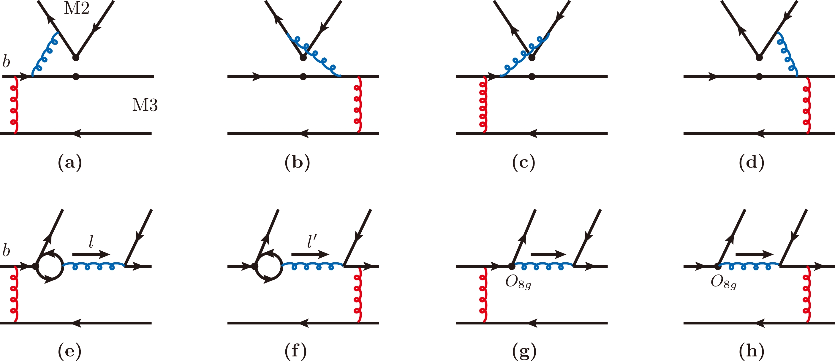
Figure 2. (color online) Typical Feynman diagrams of NLO corrections to the emission amplitudes via the vertex ((a)–(d)), quark-loop ((e)–(f)), and chromomagnetic dipole operator ((g)–(h)).
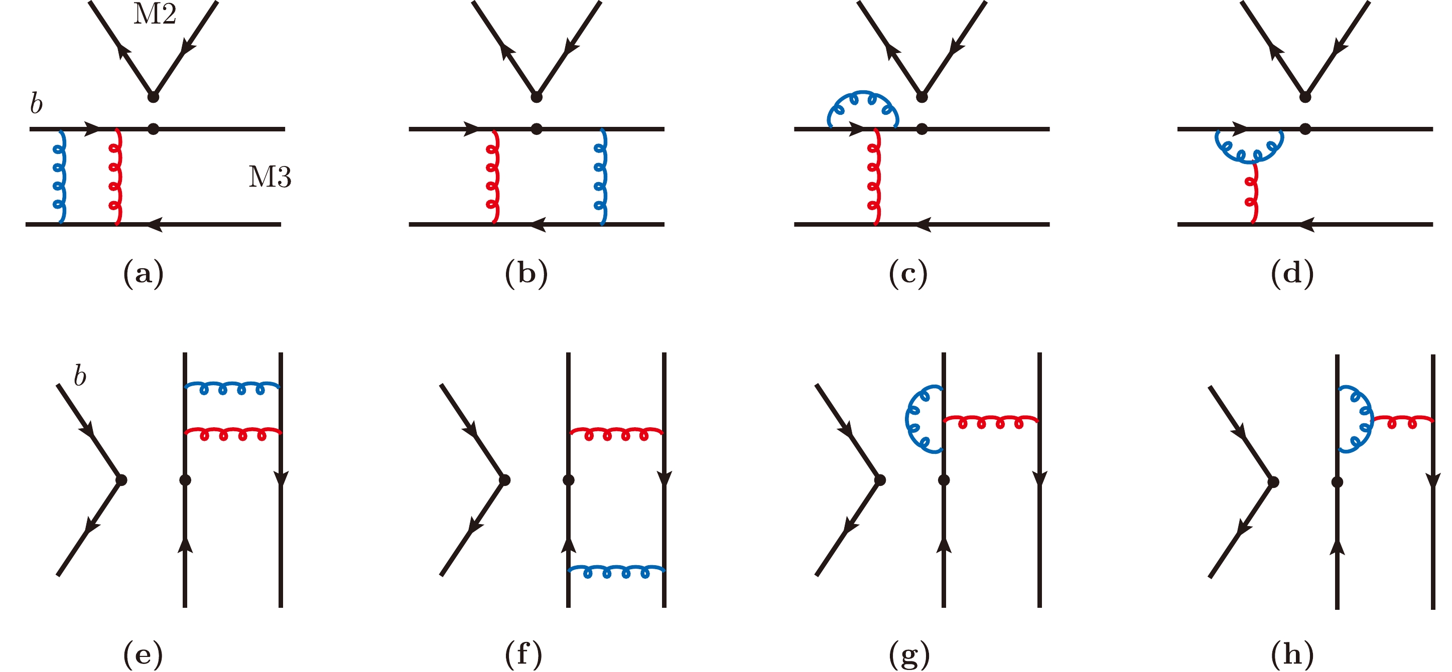
Figure 3. (color online) Typical Feynman diagrams of NLO corrections to the naive factorizable amplitudes for the
$ B \to M_2 $ transition ((a)–(d)) and timelike$ M_2 \to M_3 $ ((e)–(h)) form factor corrections.
Figure 4. (color online) Typical Feynman diagrams of NLO corrections to the hard scattering amplitudes.
-
NLO vertex corrections play an important role in reducing the dependence of Wilson coefficients on the renormalization/factorization scale. Because this type of correction does not involve the end-point singularity in the collinear factorization theorem, the results of the PQCD approach without
$ k_T $ dependence are the same as the QCDF results for vertex corrections given in Ref. [28]. The hard gluon in vertex corrections attaches two different fermion lines among the four quark operators; hence, the corrections can be absorbed into the effective Wilson coefficients according to the effective operators$ \begin{aligned}[b] a_{1,2}(\mu)\to& a_{1,2}(\mu) + \frac{\alpha_s(\mu)C_F}{4\pi} \frac{C_{1,2}(\mu)}{N_C} \, V_{1,2}(M_2) \,, \\ a_{i,i+1}(\mu) \to& a_{i,i+1}(\mu) + \frac{\alpha_s(\mu)C_F}{4\pi} \frac{C_{i+1,i}}{N_C} \, V_{i,i+1}(M_2) \\& {\rm{with}} \; i = 3,5,7,9 \,. \end{aligned} $

(70) Infrared divergence in the NLO QCD correction is factorized into the LCDAs of the emission meson. Therefore, the above NLO results are dependent on the meson type. The functions
$ V_{1,2} $ in the naive dimensional regularization scheme for the pseudoscalar meson are$ \begin{aligned}[b] V_i(P) =& 12 \ln\frac{m_b}{\mu} - 18 + \int_0^1 {\rm d} x \, \varphi_{P}^a(x) \, g(x) ~ {\rm{with}} ~ i = 1-4,9,10 \,, \\ V_i(P) =& - 12 \ln\frac{m_b}{\mu} + 6 - \int_0^1 {\rm d}x \, \varphi_{P}^a(x) \, g(1-x) ~ {\rm{with}}~ i = 5,7 \,, \end{aligned} $

$ \begin{aligned}[b]V_i(P) = - 6 + \int_0^1 {\rm d} x \, \varphi^{{\rm{p}}}_{P}(x) \, h(x) ~ {\rm{with}} ~ i = 6,8 \,, \end{aligned} $

(71) where
$ \varphi_{\rm{p}}^{(a)} $ is the LCDAs of the pseudoscalar meson. The hard kernel functions are$ \begin{aligned}[b] g(x) =& 3 \left( \frac{1-2x}{1-x} \ln x - {\rm i} \pi \right) + \Bigg[ 2 \, {\rm{Li_2}}(x) - \ln^2 x \\&+ \frac{2 \, \ln x}{1-x} + (3+2{\rm i}\pi) \, \ln x - \{ x \leftrightarrow 1-x\} \Bigg] \,, \\ h(x) =& 2 \, {\rm{Li_2}}(x) - \ln^2 x - (1+2{\rm i} \pi) \, \ln x - \{ x \leftrightarrow 1-x \} \,. \end{aligned} $

(72) When the emission particle is a vector meson, the correction functions in Eq. (71) are modified slightly by the simple substitutions of the LCDAs
$\varphi_{P}^a(x) \to \varphi_{V}^\parallel(x), \varphi_{P}^{\rm{p}}(x) \to \bar{\psi}_{V}^{s,\parallel}(x)$ .The vertex correction function contributes an imaginary part, whose effect is mainly embodied in
$ a_2, a_3 $ , and$ a_{10} $ . The Wilson coefficients$ a_3 $ and$ a_{10} $ are suppressed compared with$ a_4 $ and$ a_9 $ for the QCD penguin and electroweak penguins, respectively; hence, this correction leads to a significant change in the color-suppressed amplitudes, rather than the penguin amplitudes. For example, vertex corrections enhance the branching fraction of$ B^0 \to \pi^0\pi^0 $ by a factor of$ \sim 1.5 $ and change the sign of its direct${C P}$ violation from minus to plus, which are shown in the beginning of the next section.Besides the naive factorizable emission amplitudes shown in Figs. 2(a)–(d), the vertex correction to the hard scattering emission amplitudes is also an important part of the complete NLO results. This contribution is argued to be small in contrast with the naive factorizable ones for most charged channels. However, it is important in the color-suppressed decay channels with neutral meson final states because it may change the relative sign between the naive factorizable and hard scattering emission amplitudes, especially the imaginary parts. Further implementation of vertex correction in the annihilation topological amplitudes might provide significant changes for
${C P}$ violation with potential correction effects to the strong phase. Although the difference may be as small as estimated in Ref. [53], the direct calculation of the NLO vertex corrections in the framework of the PQCD approach is still important work to be performed in the near future. -
Because the quark-loop correction depicted in Fig. 2 (e)–(f) does not involve the end-point singularity or cause momentum redistribution in the hard kernel, the result of this NLO correction has the same form as the QCDF calculation [28].
$ \begin{eqnarray} {{\cal{C}}}^{(u,c)}(\mu, l^2) = \left[ {{\cal{G}}}^{(u,c)}(\mu, l^2) - \frac{2}{3} \right] C_2(\mu) \,, \end{eqnarray} $

(73) $ \begin{aligned}[b] {{\cal{C}}}^{(t)} (\mu, l^2)=& \left[ {{\cal{G}}}^{(s)}(\mu, l^2) - \frac{2}{3} \right] C_3(\mu) \\&+ \sum_{q^{\prime\prime}}^{u,d,s,c} {{\cal{G}}}^{(q^{\prime\prime})}(\mu, l^2) \left[ C_4(\mu) + C_6(\mu) \right] \,, \end{aligned} $

(74) where
$ l^2 $ is the invariant mass of the gluon attached to the quark loop. Here, we only include the quark-loop QCD corrections from the tree and QCD penguin operators. The quark-loop corrections from electroweak penguin operators are neglected owing to their smallness. The correction to the operator$ O_5 $ is special, with a pure ultraviolet effect, which is absorbed into the effective Wilson coefficient by the redefinition$ C_{8g}^{{\rm{eff}}} = C_{8g} + C_5 $ of the chromomagnetic dipole operator shown later. In the case of a massive charm quark①, the function$ {{\cal{G}}} $ reads as$ \begin{eqnarray} {{\cal{G}}}^{(c)}(\mu, l^2) = - 4 \int_0^1 \, {\rm d}x \, x(1-x) \ln \left[ \frac{m_c^2 - x(1-x) l^2}{\mu^2} \right] \,, \end{eqnarray} $

(75) with the real and imaginary parts
$ \begin{aligned}[b] {\rm{Re}} \left[ {{\cal{G}}}^{(c)}(\mu, l^2) \right] =& \frac{2}{3} \left( \frac{5}{3} + \frac{4 m_c^2}{l^2} - \ln \frac{m_c^2}{\mu^2} \right) + \frac{2}{3} \left( 1 + \frac{2 m_c^2}{l^2} \right) \\&\times\left\{ \begin{array}{*{20}{l}} \sqrt{\beta} \ln \dfrac{\sqrt{\beta} - 1}{\sqrt{\beta} + 1}\,, & l^2\in (- \infty, 0) \,, \\ -2 \sqrt{- \beta} \cot^{-1} \sqrt{- \beta} \,, & l^2\in [0, 4m_c^2) \,, \\ -2 \sqrt{\beta} \,, & l^2 = 4 m_c^2 \,,\\ \sqrt{\beta} \ln \dfrac{1 - \sqrt{\beta}}{1 + \sqrt{\beta}} \,, & l^2\in (4 m_c^2, \infty) \,, \end{array} \right. \, \end{aligned} $

(76) $ \begin{eqnarray} {\rm{Im}} \left[ {{\cal{G}}}^{(c)}(\mu, l^2) \right] = \frac{2 \pi}{3} \left( 1 + \frac{2 m_c^2}{l^2} \right) \sqrt{\beta} \, \Theta[\beta] \,, \end{eqnarray} $

(77) where
$ \Theta[\beta] $ is the Heaviside function. The phase space factor of the quark loop invariant mass is defined by$ \beta \equiv \beta(l^2) = 1 - 4 m_c^2/l^2 $ . We note that the above expressions with the active quark flavour number$ n_f =4 $ are slightly different from the QCDF result with$ n_f = 5 $ because the characteristic hard scale is$ {{\cal{O}}}(\sqrt{\bar{\Lambda} m_b} \sim 1.5 {\rm{GeV}}) $ in PQCD.The gluon momentum
$ l^2 $ of the quark-loop corrections is the sum of two quark momenta from two final state mesons, as shown in Fig. 2(e)–(f), which makes the decay amplitude of nonleptonic two-body$ {B} $ decays dependent on three meson wave functions,$ \begin{aligned}[b] {{\cal{M}}}^{({\rm{ql}})}_{B \to P_2 P_3} =& - \frac{8}{\sqrt{6}} C_F^2 m_B^4 \int_0^1 {\rm d}x_1{\rm d}x_2 \, {\rm d}x_3 \, \int_0^{1/\Lambda} b_1 {\rm d}b_1 \, b_3 {\rm d}b_3 \varphi_B(x_1,b_1) \, \Big\{h_{e}(x_1,x_3,b_1,b_3) E_q(\mu_q) \\ &\times\Big[ \varphi_{\pi}^a(x_2)\big[ \left(2r_b-\bar{x}_3\right)\varphi_{\pi}^a(x_3) - r_3\left(r_b-2\bar{x}_3\right)\left(\varphi_{\pi}^p(x_3)+\varphi_{\pi}^t(x_3)\right)\big] \\ & - 2r_2\varphi_{\pi}^p(x_2)\big[\left(r_b-2\right)\varphi_{\pi}^a(x_3) - r_3\left(4r_b+x_3-2\right)\varphi_{\pi}^p(x_3) +r_3x_3\varphi_{\pi}^t(x_3)\big] \Big] \\ & + h_{e}(x_3,x_1,b_3,b_1)E_{q^{\prime}}(\mu_{q^{\prime}}) \, 2 \big[ r_3\varphi_{\pi}^a(x_2)\varphi_{\pi}^p(x_3) + r_2\varphi_{\pi}^p(x_2) (x_1\varphi_{\pi}^a(x_3)+2r_3\bar{x}_1\varphi_{\pi}^p(x_3) )\big] \Big\} \,, \end{aligned} $ 
(78) $ \begin{aligned}[b] {{\cal{M}}}^{({\rm{ql}})}_{ B\to P_2V_3} =& \frac{8}{\sqrt{6}} C_F^2 m_B^4 \int_0^1 {\rm d}x_1 {\rm d}x_2 \, {\rm d}x_3 \, \int_0^{1/\Lambda} b_1 {\rm d}b_1 \, b_3 {\rm d}b_3 \varphi_B(x_1,b_1) \, \Big\{ \, h_{e}(x_1,x_3,b_1,b_3) E_q(\mu_q) \\ &\times \Big[ \varphi_{\pi}^a(x_2) \big[ \left(\bar{x}_3- 2 r_b\right)\varphi_\rho^\parallel(x_3)+r_3\left(r_b-2\bar{x}_3\right) \left(\bar{\psi}_{\rho}^{s,\parallel}(x_3)+\varphi_{\rho}^{t,\parallel}(x_3)\right) \big] \\ & - 2r_2\varphi_{\pi}^p(x_2)\big[\left(r_b-2\right)\varphi_\rho^\parallel(x_3)-r_3\left(4r_b+x_3-2\right)\bar{\psi}_{\rho}^{s,\parallel}(x_3)+r_3x_3\varphi_{\rho}^{t,\parallel}(x_3) \big] \Big] \\ &+ h_{e}(x_3,x_1,b_3,b_1)E_{q^{\prime}}(\mu_{q^{\prime}}) \, 2 \big[ -r_3 \varphi_{\pi}^a(x_2) \bar{\psi}_{\rho}^{s,\parallel}(x_3) + r_2 \varphi_{\pi}^p(x_2) (x_1 \varphi_{\rho}^{\parallel}(x_3) +2 r_3 \bar x_1 \bar{\psi}_{\rho}^{s,\parallel}(x_3) ) \big] \Big\} \,, \end{aligned} $

(79) $ \begin{eqnarray} {{\cal{M}}}^{({\rm{ql}})}_{B\to V_2P_3} &\stackrel{R}\Longleftarrow& {{\cal{M}}}^{({\rm{ql}})}_{B \to P_2 P_3} , \quad\quad\quad\quad {{\cal{M}}}^{({\rm{ql}})}_{B \to V_2V_3} \stackrel{R}\Longleftarrow {{\cal{M}}}^{({\rm{ql}})}_{ B\to P_2V_3} \,, \end{eqnarray} $

(80) $ \begin{aligned}[b] {{\cal{M}}}^{({\rm{ql}}), {\bf N}}_{B\to V_2V_3} =& -\frac{8}{\sqrt{6}} C_F^2 m_B^4 r_2 \int_0^1 {\rm d}x_1 {\rm d}x_2 \, {\rm d}x_3 \, \int_0^{1/\Lambda} b_1 {\rm d}b_1 \, b_3 {\rm d}b_3 \varphi_B(x_1,b_1)\, \Big\{ h_{e}(x_1,x_3,b_1,b_3) E_q(\mu_q) \\ &\times\Big[ r_3\big[(4r_b+x_3-2)\left(\bar{\psi}_{\rho}^{s,\perp}(x_2)\bar{\psi}_{\rho}^{s,\perp}(x_3) +\varphi_{\rho}^{t,\perp}(x_2)\varphi_{\rho}^{t,\perp}(x_3)\right) - x_3\left(\bar{\psi}_{\rho}^{s,\perp}(x_2)\varphi_{\rho}^{t,\perp}(x_3)+\varphi_{\rho}^{t,\perp}(x_2)\bar{\psi}_{\rho}^{s,\perp}(x_3)\right) \\ & - (r_b-2)\varphi_{\rho}^{\perp}(x_3)\left(\bar{\psi}_{\rho}^{s,\perp}(x_2)+\varphi_{\rho}^{t,\perp}(x_2)\right)\big]\Big] + h_{e}(x_3,x_1,b_3,b_1)E_{q^{\prime}}(\mu_{q^{\prime}}) \, r_3\Big[\bar{\psi}_{\rho}^{s,\perp}(x_2)\left(\bar{x}_1\bar{\psi}_{\rho}^{s,\perp}(x_3)+(1+x_1)\varphi_{\rho}^{t,\perp}(x_3)\right) \\& + \varphi_{\rho}^{t,\perp}(x_2)\left((1+x_1)\bar{\psi}_{\rho}^{s,\perp}(x_3)+\bar{x}_1\varphi_{\rho}^{t,\perp}(x_3)\right)\Big]\Big\} \,, \\[-12pt]\end{aligned} $

(81) $ \begin{aligned}[b] {{\cal{M}}}^{({\rm{ql}}), {\bf T}}_{B\to V_2V_3} =& -\frac{8}{\sqrt{6}} C_F^2 m_B^4 r_2 \int_0^1 {\rm d}x_1{\rm d}x_2 \, {\rm d}x_3 \, \int_0^{1/\Lambda} b_1 {\rm d}b_1 \, b_3 {\rm d}b_3 \varphi_B(x_1,b_1)\, \Big\{ \, h_{e}(x_1,x_3,b_1,b_3) E_q(\mu_q) \\ &\times \Big[r_3 \big[ x_3\left(\varphi_{\rho}^{t,\perp}(x_2)-\bar{\psi}_{\rho}^{s,\perp}(x_2)\right)\left(\bar{\psi}_{\rho}^{s,\perp}(x_3)-\varphi_{\rho}^{t,\perp}(x_3)\right) + 2(2 r_b-1)\left(\bar{\psi}_{\rho}^{s,\perp}(x_2)\varphi_{\rho}^{t,\perp}(x_3)+\varphi_{\rho}^{t,\perp}(x_2)\bar{\psi}_{\rho}^{s,\perp}(x_3)\right) \big] \\ & - (r_b-2)\varphi_{\rho}^{\perp}(x_3)\left(\bar{\psi}_{\rho}^{s,\perp}(x_2)+\varphi_{\rho}^{t,\perp}(x_2)\right) \Big] + h_{e}(x_3,x_1,b_3,b_1)E_{q^{\prime}}(\mu_{q^{\prime}}) \,r_3 \Big[ \bar{\psi}_{\rho}^{s,\perp}(x_2) \big[ (1+x_1)\bar{\psi}_{\rho}^{s,\perp}(x_3)+\bar{x}_1\varphi_{\rho}^{t,\perp}(x_3) \big] \\ & + \varphi_{\rho}^{t,\perp}(x_2) \big[ \bar{x}_1\bar{\psi}_{\rho}^{s,\perp}(x_3)+(1+x_1)\varphi_{\rho}^{t,\perp}(x_3) \big] \Big] \Big\} \,. \\[-12pt] \end{aligned} $

(82) The Sudakov factor functions
$ E_{q^{(\prime)}} $ in these amplitudes are also collected in Appendix A. -
As depicted in Fig. 2(g) and (h), the chromomagnetic dipole operator
$ O_{\rm{8g}} $ contributes another NLO correction. Similar to the quark-loop corrections, it introduces another independent amplitude to two body B decays.$ \begin{aligned}[b] {{\cal{M}}}^{({\rm{mp}})}_{B\to P_2P_3} =& -\frac{8}{\sqrt{6}} C_F^2 m_B^6 \int_0^1 {\rm d}x_1 {\rm d}x_2\, {\rm d}x_3 \, \int_0^{1/\Lambda} b_1 {\rm d}b_1 b_2 {\rm d}b_2 \, b_3 {\rm d}b_3 \varphi_B(x_1,b_1) \cdot\Big\{ h_g(\alpha_g,\beta_g,\gamma_g,b_1,b_2,b_3) E_{8g}(\mu_g) \\&\times \Big[-\bar{x}_3\varphi_{\pi}^a(x_2)\Big(2(r_b-2)\varphi_{\pi}^a(x_3) +r_3 \big[ \varphi_{\pi}^t(x_3)(-2r_b+x_3+1)- \varphi_{\pi}^p(x_3)\left(6r_b-\bar{x}_3\right) \big] \Big) \\ & +r_2 \big[ x_2\left(3\varphi_{\pi}^p(x_2)-\varphi_{\pi}^t(x_2)\right) \big(\varphi_{\pi}^a(x_3)(2r_b-\bar{x}_3)-r_3(r_b-2\bar{x}_3) \left(\varphi_{\pi}^p(x_3)+\varphi_{\pi}^t(x_3)\right)\Big) \\& - r_3(r_b-2)\bar{x}_3\left(3\varphi_{\pi}^p(x_2)+\varphi_{\pi}^t(x_2)\right)\left(\varphi_{\pi}^p(x_3)-\varphi_{\pi}^t(x_3)\right) \big] \Big] \\ & + h_g(\alpha_{g^\prime},\beta_{g^\prime},\gamma_{g^\prime},b_1,b_2,b_3) E_{8g^{\prime}}(\mu_{g^{\prime}}) \Big[x_1\varphi_{\pi}^a(x_3)\big[ \varphi_{\pi}^a(x_2)+r_2\left(3\varphi_{\pi}^p(x_2)+\varphi_{\pi}^t(x_2)\right)\Big] \end{aligned} $ 
$ \begin{aligned}[b] \quad\quad\quad\quad- 2 r_3\varphi_{\pi}^p(x_3) \big[(x_1-2)\varphi_{\pi}^a(x_2)+r_2\left(6x_1\varphi_{\pi}^p(x_2)+x_2\left(\varphi_{\pi}^t(x_2)-3\varphi_{\pi}^p(x_2)\right)\right)\big] \Big]\Big\} \,, \end{aligned} $

(83) $ \begin{aligned}[b] {{\cal{M}}}^{({\rm{mp}})}_{B\to P_2V_3} =& \frac{8}{\sqrt{6}} C_F^2 m_B^6 \int_0^1 {\rm d}x_1 {\rm d}x_2\, {\rm d}x_3 \, \int_0^{1/\Lambda} b_1 {\rm d}b_1 b_2 {\rm d}b_2 \, b_3 {\rm d}b_3 \varphi_B(x_1,b_1)\, \Big\{ h_g(\alpha_g,\beta_g,\gamma_g,b_1,b_2,b_3) E_{8g}(\mu_g)\\&\times\Big[ \bar{x}_3\varphi_{\pi}^a(x_2)\Big(2(r_b-2)\varphi_\rho^\parallel(x_3) + r_3\big[ \varphi_{\rho}^{t,\parallel}(x_3)(-2r_b+x_3+1) - \bar{\psi}_\rho^{s,\parallel}(x_2)\left(6r_b-\bar x_3 \right) \Big) \big] \\ & + r_2 \big[ x_2\left(3\varphi_{\pi}^p(x_2)-\varphi_{\pi}^t(x_2)\right)\big(\varphi_\rho^\parallel(x_3)(2r_b-\bar{x}_3) - r_3(r_b-2\bar{x}_3) (\bar{\psi}_\rho^{s,\parallel}(x_2)+\varphi_{\rho}^{t,\parallel}(x_3) )\big) \\ &+ r_3(r_b-2)\bar{x}_3\left(3\varphi_{\pi}^p(x_2)+\varphi_{\pi}^t(x_2)\right)\left( \varphi_{\rho}^{t,\parallel}(x_3)-\bar{\psi}_\rho^{s,\parallel}(x_3)\right) \big] \Big] \\ & + h_g(\alpha_{g^\prime},\beta_{g^\prime},\gamma_{g^\prime},b_1,b_2,b_3)E_{8g^{\prime}}(\mu_{g^{\prime}}) \Big[x_1\varphi_\rho^\parallel(x_3)\big[ r_2\left(3\varphi_{\pi}^p(x_2)+\varphi_{\pi}^t(x_2)\right)-\varphi_{\pi}^a(x_2) \big] \\ & + 2 r_3\bar{\psi}_\rho^{s,\parallel}(x_3)\big[ (x_1-2)\varphi_{\pi}^a(x_2)-r_2\left(6x_1\varphi_{\pi}^p(x_2)+x_2\left(\varphi_{\pi}^t(x_2)-3\varphi_{\pi}^p(x_2)\right)\right)\big] \Big]\Big\} \,, \end{aligned} $

(84) $ \begin{aligned}[b] {{\cal{M}}}^{({\rm{mp}}), {\bf N}}_{B\to V_2V_3}=& -\frac{8}{\sqrt{6}} C_F^2 m_B^6 \int_0^1 {\rm d}x_1{\rm d}x_2 \, {\rm d}x_3 \, \int_0^{1/\Lambda} b_1 {\rm d}b_1 b_2 {\rm d}b_2 \, b_3 {\rm d}b_3 \varphi_B(x_1,b_1)\,\cdot \Big\{ h_g(\alpha_g,\beta_g,\gamma_g,b_1,b_2,b_3) E_{8g}(\mu_g) \\ & \Big[r_2 r_3\Big( \big[ 2\left(1+x_2\right)\bar{x}_3-r_b\left(x_2+\bar{x}_3\right) \big] \big[ \bar{\psi}_{\rho}^{s,\perp}(x_2)\bar{\psi}_{\rho}^{s,\perp}(x_3) + \varphi_{\rho}^{t,\perp}(x_2)\varphi_{\rho}^{t,\perp}(x_3)\big] \\ &- \big[ 2\bar{x}_2\bar{x}_3+r_b\left(x_2-\bar{x}_3\right)\big] \big[\bar{\psi}_{\rho}^{s,\perp}(x_2)\varphi_{\rho}^{t,\perp}(x_3)+\varphi_{\rho}^{t,\perp}(x_2)\bar{\psi}_{\rho}^{s,\perp}(x_3)\big]\Big) \\ & + \left( \bar{x}_3-2r_b \right) \big[ r_3\bar{x}_3\varphi_{\rho}^{\perp}(x_2)\left(\bar{\psi}_{\rho}^{s,\perp}(x_3)-\varphi_{\rho}^{t,\perp}(x_3)\right) - r_2x_2\varphi_{\rho}^{\perp}(x_3)\left(\bar{\psi}_{\rho}^{s,\perp}(x_2)+\varphi_{\rho}^{t,\perp}(x_2)\right) \big] \Big] \\ & + h_g(\alpha_{g^\prime},\beta_{g^\prime},\gamma_{g^\prime},b_1,b_2,b_3) E_{8g^{\prime}}(\mu_{g^{\prime}}) \, r_3 \Big[ x_1\varphi_{\rho}^{\perp}(x_2)\left(\bar{\psi}_{\rho}^{s,\perp}(x_3)-\varphi_{\rho}^{t,\perp}(x_3)\right) \\ & + r_2\big[ x_2\left(\bar{\psi}_{\rho}^{s,\perp}(x_2)+\varphi_{\rho}^{t,\perp}(x_2)\right) \left(\bar{\psi}_{\rho}^{s,\perp}(x_3)+\varphi_{\rho}^{t,\perp}(x_3)\right) - 2x_1\left(\bar{\psi}_{\rho}^{s,\perp}(x_2)\bar{\psi}_{\rho}^{s,\perp}(x_3)+\varphi_{\rho}^{t,\perp}(x_2)\varphi_{\rho}^{t,\perp}(x_3)\right)\big] \Big] \Big\} \,, \end{aligned} $

(85) $ \begin{aligned}[b] {{\cal{M}}}^{({\rm{mp}}), {\bf T}}_{B\to V_2V_3} =& -\frac{8}{\sqrt{6}} C_F^2 m_B^6 \int_0^1 {\rm d}x_1{\rm d}x_2 \, {\rm d}x_3 \, \int_0^{1/\Lambda} b_1 {\rm d}b_1 b_2 {\rm d}b_2 \, b_3 {\rm d}b_3 \varphi_B(x_1,b_1)\, \cdot \Big\{h_g(\alpha_g,\beta_g,\gamma_g,b_1,b_2,b_3) E_{8g}(\mu_g) \\ &\times \Big[r_2 r_3\Big(-[ 2\bar{x}_2\bar{x}_3+r_b\left(x_2-\bar{x}_3\right) \big] \big[ \bar{\psi}_{\rho}^{s,\perp}(x_2)\bar{\psi}_{\rho}^{s,\perp}(x_3) + \varphi_{\rho}^{t,\perp}(x_2)\varphi_{\rho}^{t,\perp}(x_3) \big] \\ & + \big[ 2\left(1+x_2 \right)\bar{x}_3-r_b\left(x_2+\bar{x}_3\right)\big] \big[ \bar{\psi}_{\rho}^{s,\perp}(x_2)\varphi_{\rho}^{t,\perp}(x_3)+\varphi_{\rho}^{t,\perp}(x_2)\bar{\psi}_{\rho}^{s,\perp}(x_3)\big] \Big) \\ & + \left(\bar{x}_3-2r_b\right) \big[ r_3\bar{x}_3\varphi_{\rho}^{\perp}(x_2)\left(\bar{\psi}_{\rho}^{s,\perp}(x_3)-\varphi_{\rho}^{t,\perp}(x_3)\right) - r_2x_2\varphi_{\rho}^{\perp}(x_3)\left(\bar{\psi}_{\rho}^{s,\perp}(x_2)+\varphi_{\rho}^{t,\perp}(x_2)\right) \big] \Big] \\ & + h_g(\alpha_{g^\prime},\beta_{g^\prime},\gamma_{g^\prime},b_1,b_2,b_3) E_{8g^{\prime}}(\mu_{g^{\prime}}) \, r_3 \Big[ x_1\varphi_{\rho}^{\perp}(x_2)\left(\bar{\psi}_{\rho}^{s,\perp}(x_3)-\varphi_{\rho}^{t,\perp}(x_3)\right) \\ &+ r_2\big[ x_2\left(\bar{\psi}_{\rho}^{s,\perp}(x_2)+\varphi_{\rho}^{t,\perp}(x_2)\right) \left(\bar{\psi}_{\rho}^{s,\perp}(x_3)+\varphi_{\rho}^{t,\perp}(x_3)\right) - 2x_1\left(\bar{\psi}_{\rho}^{s,\perp}(x_2)\varphi_{\rho}^{t,\perp}(x_3)+\varphi_{\rho}^{t,\perp}(x_2)\bar{\psi}_{\rho}^{s,\perp}(x_3)\right)\big] \Big] \Big\} \,, \end{aligned} $

(86) $ \begin{eqnarray} {{\cal{M}}}^{({\rm{mp}})}_{B\to V_2P_3} &\stackrel{R}\Longleftarrow& {{\cal{M}}}^{({\rm{mp}})}_{B\to P_2P_3} \,, \quad {{\cal{M}}}^{({\rm{mp}})}_{B\to V_2V_3} \stackrel{R}\Longleftarrow {{\cal{M}}}^{({\rm{mp}})}_{B\to P_2V_3} \,. \end{eqnarray} $

(87) The hard functions in these decay amplitudes are also collected in Appendix A.
-
The NLO QCD corrections to the naive factorizable diagrams of hadronic B decays are the same as the
$ B \to \pi $ transition form factors. The typical Feynman diagrams shown in the first row of Fig. 3 are calculated in the framework of$ k_T $ factorization [55, 56]. The resulting NLO correction kernels are of the following form:$ \begin{aligned}[b] {\rm{F_{T2}}^{(1)}}(x_i, \zeta_3) =& \frac{\alpha_s(\mu_f)C_F}{4\pi} \Bigg[ \frac{21}{4}\ln \frac{\mu^2}{m_B^2} - \left( \ln \frac{m_B^2}{\zeta_1^2} + \frac{13}{2} \right) \ln \frac{\mu_f^2}{m_B^2} + \frac{7}{16} \ln^2(x_1x_3) + \frac{1}{8} \ln^2 x_1 + \frac{1}{4} \ln x_1 \ln x_3 \\&+ \left( 2 \ln \frac{m_B^2}{\zeta_1^2} - \frac{1}{4} \right) \ln x_1 - \frac{3}{2} \ln x_3 - \left( \frac{3}{2} \ln \frac{m_B^2}{\zeta_1^2} + 1 \right) \ln \frac{m_B^2}{\zeta_1^2} + \frac{101}{48} \pi^2 + \frac{219}{16} \Bigg] \,, \end{aligned} $ 
(88) $ \begin{aligned}[b] {\rm{F_{T3}}^{(1)}}(x_i, \zeta_3 )=& \frac{\alpha_s(\mu_f)C_F}{4\pi} \Bigg[ \frac{21}{4}\ln \frac{\mu^{\prime 2}}{m_B^2} - \left( \frac{1}{2} \ln \frac{m_B^2}{\zeta_1^2} + 3 \right) \ln \frac{\mu_f^2}{m_B^2} + \frac{7}{16} \ln^2 x_1 - \frac{3}{8} \ln^2 x_3 + \frac{9}{8} \ln x_1 \ln x_3 \\&+ \left( \ln \frac{m_B^2}{\zeta_1^2} - \frac{29}{8} \right) \ln x_1 + \ln \frac{m_B^2}{\zeta_3^2} + \left( \ln \frac{m_B^2}{\zeta_3^2} - \frac{25}{16} \right) \ln x_3 - \left( \frac{1}{4} \ln \frac{m_B^2}{\zeta_1^2} - \frac{1}{2} \right) \ln \frac{m_B^2}{\zeta_1^2} + \frac{37}{32} \pi^2 + \frac{91}{32} \Bigg] \, . \end{aligned} $

(89) To evade light-cone singularities in the above calculations, we introduce the dimensional parameters
$ \zeta_1^2 \equiv 4 (n_1 \cdot p_1)^2/\vert n_1^2 \vert $ and$ \zeta_3^2 \equiv 4 (n_3 \cdot p_3)^2/\vert n_3^2 \vert $ by varying the Wilson links in the transverse momentum dependent definition of mesons away from the light-cone ($ n_1^2, n_3^2 \neq 0 $ ). These additional scales introduce another scheme dependence known as rapidity singularities, which, in principle, should be resummed to all orders by resolving the evolution equation of B and π meson wave functions on the dimensionless scales$ \zeta_1^2/m_B^2 $ and$ \zeta_3^2/m_B^2 $ , respectively. The solutions demonstrate that the resummation effect suppresses the shape of theB meson LCDA $ \varphi_+(k^+, b, \mu) $ near the endpoint$ k^+ \to 0 $ [118], and the dependence on the choice of$ \zeta_3 $ is not significant in pion meson wave functions because the joint resummation-improved pion wave function does not exhibit sizable corrections [119]. This is not accidental because the$ k_T $ and threshold resummations have previously reshaped the end-point behaviours of meson wave functions [65]. For the sake of simplicity, we can take$ \zeta_3^2 = m_B^2 $ to eliminate the logarithm term$ \ln (\zeta_3^2/m_B^2) $ and take a large value of$ \zeta_1^2 $ at$ 25^2 m_B^2 $ to reduce the uncertainty on the constant terms from the loop calculation in different momentum regions.The factorization scale in NLO kernels is chosen on the hard scale in the corresponding decay amplitudes, and the choice of renormalization scale is purposed to eliminate all single logarithms, with the same argument to reduce the uncertainties as much as possible.
$ \begin{eqnarray} \mu \equiv \mu(\mu_f) =\Big\{ {\rm{Exp}} \Big[ c_1 + \left( \ln \frac{m_B^2}{\zeta_1^2} + \frac{5}{4} \right) \ln \frac{\mu_f^2}{m_B^2} \Big] x_1^{c_2} x_2^{c_3}\Big\}^{2/21} \mu_f \,, \end{eqnarray} $

(90) $ \begin{eqnarray} \mu^\prime \equiv \mu^\prime(\mu_f) = \Big\{ {\rm{Exp}} \Big[ c^\prime_1 + \left( \frac{1}{2}\ln \frac{m_B^2}{\zeta_1^2} - \frac{9}{4} \right) \ln \frac{\mu_f^2}{m_B^2} \Big] x_1^{c_2^\prime} x_2^{c_3^\prime}\Big\}^{2/21} \mu_f \,. \end{eqnarray} $

(91) The parameters entered into Eqs. (90) and (91) are
$ \begin{aligned}[b] c_1 =& \left( \frac{3}{2} \ln \frac{m_B^2}{\zeta_1^2} + 1 \right) \ln \frac{m_B^2}{\zeta_1^2} - \frac{101}{48} \pi^2 - \frac{219}{16} \,, \\ c_2 =& - \left( 2 \ln \frac{m_B^2}{\zeta_1^2} - \frac{1}{4} \right) \,, \quad c_3 = + \frac{3}{2} \,, \end{aligned} $

$ \begin{aligned}[b] c_1^\prime =& \left( \frac{1}{4} \ln \frac{m_B^2}{\zeta_1^2} - \frac{1}{2} \right) \ln \frac{m_B^2}{\zeta_1^2} - \frac{37}{32} \pi^2 - \frac{91}{32} \,, \\ c_2^\prime =& - \left( \ln \frac{m_B^2}{\zeta_1^2} - \frac{29}{8} \right) \,, \quad c_3^\prime = + \frac{25}{16} \,, \end{aligned} $

(92) We note that the kernels
$ {\rm{F_{T2}}^{(1)}} $ and$ {\rm{F_{T3}}^{(1)}} $ are the corrections to the decay amplitude of naive factorizable emission diagrams in$ B \to PP $ decays, as shown in Eq. (38), which are attached to the terms proportional to the leading twist π meson LCDA$ \varphi_\pi $ and twist-3 LCDA$ \varphi_\pi^p $ , respectively. The NLO expression is modified to$ \begin{aligned}[b] {\cal{E}}_{M_3}^{{\bf{LL}}, {\rm{NLO}}} =& -{\cal{E}}_{M_3}^{{\bf{LR}}, {\rm{NLO}}}= 8 \pi C_F m_B^4 f_{M_2} \int_0^1 {\rm d}x_1 \, {\rm d}x_3 \, \\&\times\int_0^{1/\Lambda} b_1 {\rm d}b_1 \, b_3 {\rm d}b_3 \varphi_B(x_1,b_1)\, \\ &\cdot \Big\{ h_{e}(x_1,x_3,b_1,b_3) E_e(\mu_e) \Big[ (2\,r_b-\bar{x}_3)\\&\times \left[ 1 + {\rm{F_{T2}}^{(1)}}(x_i, \zeta_3) \right] \varphi_{\pi}^a(x_3) \\ & - r_3\left(r_b-2\bar{x}_3 \right)\left(\varphi_{\pi}^p(x_3)+\varphi_{\pi}^t(x_3)\right) \Big] \\ & + h_{e}(x_3,x_1,b_3,b_1) E_{e^{\prime}}(\mu_{e^{\prime}}) \,2\,r_3\\&\times \left[ 1 + {\rm{F_{T3}}^{(1)}}(x_i, \zeta_3) \right] \varphi_{\pi}^p(x_3) \Big\} \,. \end{aligned} $

(93) The following comments are made:
$ (1) $ The ultraviolet divergence at NLO is treated by the traditional renormalization group technique in the$ \overline{{\rm{MS}}} $ scheme. It is regulated by the counter terms of quark fields and the strong coupling constant.$ (2) $ The infrared divergences are regulated by the transverse momenta of light quarks and the soft gluon mass, where the latter is introduced to protect the b quark on shell required by the standard effective heavy field in the$ k_T $ factorization theorem. The cancelation of infrared divergences occurs between the QCD quark diagrams and the effective diagrams of meson wave functions, up to sub-leading twist LCDAs of pions. The retaining infrared finite NLO hard kernel still has large logarithms, in which the double logarithms in terms of$ \ln^2 (x_i) $ are resummed to the threshold Sudakov exponent, and the single logarithm$ \ln(x_i) $ can be diminished by the choice of renormalization scale to the physical mass.$ (3) $ The infrared finite NLO hard kernel is$ k_T $ dependent because it is obtained by taking the difference of the NLO quark amplitude and the convolution of NLO wave functions with the LO hard kernel. Meanwhile, the small$ k_T $ contribution is highly suppressed by the$ k_T $ resummed wave functions.$ (4) $ From the phenomenological side, the$ \sim 30$ % enhancement from NLO correction with the leading twist distribution amplitude of pion mesons is partly canceled by the$ \sim 20$ % decrease in NLO correction with the sub-leading twist distribution amplitude. Therefore, this results in an approximately$ 8$ % NLO correction to the LO contributions of$ B \to \pi $ transition form factors.In fact, only the NLO correction for the
$ B \to \pi $ transition form factors induced by the vector current is complete. NLO calculations for the$ B \to \pi $ transition induced by the scalar quark current and those for the$ B \to \rho $ transition are still absent. Further effort is clearly required. -
Regarding color suppressed channels with the W-exchange diagram contribution, such as
$ B^0 \to \pi^0\pi^0, \pi^0 \eta_q, \eta_q\eta_q $ , annihilation type amplitudes provide not only the main source of large${C P}$ asymmetry, but also an indispensable contribution to the total decay amplitude. Annihilation amplitudes are more important than emission amplitudes when the strong destructive interaction between the color suppressed tree amplitude${{C}}$ and the penguin amplitude${{P}}$ becomes true. The NLO QCD corrections to the naive factorizable annihilation amplitudes have been calculated to improve the PQCD precision for relevant B meson decays [57–61]. The most important contribution of this type of NLO correction is the timelike form factors, as depicted in the second row of Fig. 3, and the NLO hard kernels are quoted as [57, 58]$ \begin{aligned}[b] {\rm{G}}_{\pi, {\rm{T2}}}^{(1)} =& \frac{\alpha_s(\mu) C_F}{4 \pi} \Big[ -\frac{3}{4} \ln \frac{\mu^2}{m_B^2} - \frac{1}{4} \ln^2 \left(\frac{4x_2x_3}{m_B^2b_2^2}\right) - \frac{17}{4} \ln^2 x_3 + \frac{27}{8} \ln x_2 \ln x_3 + \left( \frac{17}{8} \ln x_3 + \frac{23}{16} + \gamma_E + {\rm i} \frac{\pi}{2} \right) \ln \left( \frac{4x_2x_3}{m_B^2b_2^2} \right)\\& - \left( \frac{13}{8} + \frac{17}{4} \gamma_E - {\rm i} \frac{17}{8} \pi \right) \ln x_3 + \frac{31}{16} \ln x_2 - \frac{\pi^2}{2} + (1 - 2 \gamma_E) \pi + \frac{\ln 2}{2} + \frac{53}{4} - \frac{23 \gamma_E}{8} - \gamma_E^2 + {\rm i} \pi \left( \frac{171}{16} + \gamma_E \right) \Big] \,, \end{aligned} $ 
(94) $ \begin{eqnarray} {\rm{G}}_{\pi, {\rm{T3, 1}}}^{(1)} = \frac{\alpha_s(\mu) C_F}{4 \pi} \Big[ \frac{9}{4} \ln \frac{\mu^2}{m_B^2} - \frac{53}{32} \ln \left(\frac{4x_2x_3}{m_B^2b_2^2} \right) - \frac{23}{32} \ln \left( \frac{4x_3}{m_B^2b_3^2}\right) - \frac{1}{8} \ln^2 x_2 - \frac{9}{8} \ln x_2 - \frac{137}{96} \pi^2 + \frac{19}{4} \gamma_E + \frac{337}{64} + {\rm i} \pi \frac{39}{8} \Big] \,, \end{eqnarray} $

(95) $ \begin{aligned}[b] {\rm{G}}_{\pi, {\rm{T3, 2}}}^{(1)} =& \frac{\alpha_s(\mu) C_F}{4 \pi} \Bigg[ \frac{9}{4} \ln \frac{\mu^2}{m_B^2} - 2 \ln \left(\frac{4x_2x_3}{m_B^2b_2^2} \right) - \frac{1}{8} \ln^2 \left( \frac{4x_3}{m_B^2b_3^2}\right) + \left( \frac{\gamma_E}{2} + \frac{3}{4} {\rm i} \pi \right) \ln \left( \frac{4x_3}{m_B^2b_3^2}\right) \\ &+ 2\ln x_2 - \frac{\pi^2}{4} - \frac{\gamma_E^2}{2} + 4 \gamma_E + \frac{\ln 2}{4} + \frac{11}{2} + {\rm i} \pi \left( \frac{15}{4} - \frac{3}{2} \gamma_E \right)\Bigg]\,. \end{aligned} $

(96) The
$ B \to PP $ decay amplitudes with the$ {\rm{(V-A) \otimes (V \pm A)}} $ current in the naive factorizable annihilation diagrams at NLO accuracy are then modified to$ \begin{aligned}[b] {\cal{A}}^{{\bf{LL}}, {\rm{NLO}}}_{M_3}=&{\cal{A}}^{{\bf{LR}}, {\rm{NLO}}}_{M_3}= 8 \pi C_F m_B^4 f_B \int_0^1 \,{\rm d}x_2 \, {\rm d}x_3 \, \int_0^{1/ \Lambda} b_2 {\rm d}b_2 \, b_3 {\rm d}b_3 \\ &\cdot \Big\{ h_{a}(x_2,{\bar x}_3,b_2,b_3)E_a({\mu_a}) \Big[ -\bar{x}_3 \left( 1 + {\rm{G}}_{\pi, {\rm{T2}}}^{(1)} \right) \varphi_{\pi}^a(x_2)\varphi_{\pi}^a(x_3) + 2r_2r_3 \varphi_{\pi}^p(x_2) \\ & \cdot \big[ - \left( 1 + {\rm{G}}_{\pi, {\rm{T3, 2}}}^{(1)} \right) \left( \varphi_{\pi}^p(x_3) + \varphi_{\pi}^t(x_3) \right) + {\bar x}_3 \left( 1 + {\rm{G}}_{\pi, {\rm{T3, 1}}}^{(1)} \right) \left( \varphi_{\pi}^t(x_3) - \varphi_{\pi}^p(x_3) \right) \big] \Big] \\ & + h_{a}({\bar x}_3,x_2,b_3,b_2) E_{a^\prime}({\mu_{a^\prime}}) \Big[ x_2 \left( 1 + {\rm{G}}_{\pi, {\rm{T2}}}^{(1)} \right) \varphi_{\pi}^a(x_2)\varphi_{\pi}^a(x_3) + 2r_2r_3 \varphi_{\pi}^p(x_3) \\ & \cdot \big[\left( 1 + {\rm{G}}_{\pi, {\rm{T3, 1}}}^{(1)} \right) \left( \varphi_{\pi}^p(x_2) - \varphi_{\pi}^t(x_2) \right) + x_2 \left( 1 + {\rm{G}}_{\pi, {\rm{T3, 2}}}^{(1)} \right) \left( \varphi_{\pi}^p(x_2) + \varphi_{\pi}^t(x_2) \right) \big] \Big]\Big\} \,. \end{aligned} $

(97) This correction does not bring the contribution to the decaying channels with two identical mesons in the final states. However, its contribution to the channels
$ B^0 \to \pi^0 \eta, \pi^0 \eta^\prime $ may be expected as approximately$ 30 $ % with the general recognition of$S U(3)$ flavor breaking.For the channel
$ B^0 \to \pi^0 \pi^0 $ ,$ {{\cal{A}}}^{{\bf LL}} = {{\cal{A}}}^{{\bf LR}} = 0 $ , and hence naive factorizable annihilation only stems from the$ {\rm{(S+P) \otimes (S-P)}} $ current with the amplitude$ {{\cal{A}}}^{\bf SP} $ , as given in Eq. (43). Considering NLO correction, this part of the decay amplitude is modified to$ \begin{aligned}[b] {\cal{A}}^{{\bf{SP}}}_{M_3}=& 16 \pi C_F m_B^4 f_B \int_0^1 \,{\rm d}x_2 \, {\rm d}x_3 \, \int_0^{1/\Lambda} b_2 {\rm d}b_2 \, b_3 {\rm d} b_3\cdot \Big\{ h_{a}(x_2,{\bar x}_3,b_2,b_3)E_a({\mu_a}) \Big[ r_3\bar{x}_3\varphi_{\pi}^a(x_2) \left( \varphi_{\pi}^p(x_3)+\varphi_{\pi}^t(x_3)\right) \\&+ 2 r_2 \left( 1 + \Gamma^{(1)}(Q^2)\right) \varphi_{\pi}^p(x_2)\varphi_{\pi}^a(x_3) \Big] + h_{a}({\bar x}_3,x_2,b_3,b_2)E_{a^\prime}({\mu_{a^\prime}}) \Big[ r_2 x_2\varphi_{\pi}^a(x_3)\left(\varphi_{\pi}^p(x_2)-\varphi_{\pi}^t(x_2)\right) \\&+ 2 r_3 \left( 1 + \Gamma^{(1)}(Q^2)\right) \varphi_{\pi}^a(x_2)\varphi_{\pi}^p(x_2) \Big]\Big\} \, \end{aligned} $

(98) with the correction kernel function [59]
$ \begin{aligned}[b] \Gamma^{(1)}=& \frac{\alpha_s C_F}{8\pi} \Big\{ \frac{5}{2} \ln \frac{\mu^2}{m_B^2} - \frac{1}{16} \ln^2 \left( \frac{4 x_2 (1-x_3)}{m_B^2 b_3^2} \right) + \left( \frac{33}{8} - \frac{\gamma_E}{4} \right) \ln \left( \frac{4 x_2 (1-x_3)}{m_B^2 b_3^2} \right) - \ln^2 (1-x_3) - \frac{3}{8} \ln^2 x_2 \\&+ \frac{1}{2} \ln x_2 \ln (1-x_3) - \frac{71}{4} \ln (1-x_3) - \frac{7}{4} \ln x_2 - \frac{105}{48} \pi^2 + \frac{41}{2} - \frac{\gamma_E^2}{2} - \frac{33 \gamma_E}{4} + {\rm i} \pi \frac{5}{2} \Big\} \,. \end{aligned} $

(99) For the timelike scalar pion form factor, the positive real part and negative imaginary part at LO play a dominant role in producing large
$ {C P} $ asymmetry in$ B^0 \to \pi^0\pi^0 $ decay. The numerical results show that the NLO contribution is small in both the magnitude and phase, which is only slightly different from the LO PQCD predictions for$ B \to \pi\pi $ decays.The timelike
$ \rho\pi $ electromagnetic form factor is also studied at NLO in the framework of$ k_T $ factorization [61]. In$ B \to \rho\pi $ decays, it is found that the contribution proportional to the timelike electromagnetic form factor is power suppressed even at LO, which can be neglected in numerical calculations. The leading power contribution to the annihilation amplitude originates from the timelike$ \rho\pi $ transition form factor induced by the axial-vector current and pseudoscalar density operators, whose NLO correction is unknown at present. -
In previous sections, we present various NLO contributions for two body B meson decays. These corrections along with LO perturbation calculations are channel dependent, which are shown as different effective four quark operators involved in different B meson decay channels. With the inclusion of the various types of NLO corrections presented above, the total decay amplitudes for different
$ B \to PP $ channels are presented as follows:$ \begin{aligned}[b] {{\cal{M}}}(B^+ \to \pi^+ K^0) =& \frac{G_F}{\sqrt{2}} V^{\ast}_{ub} V_{us} \Big[ a_1 {{\cal{A}}}_{\pi}^{{\bf LL}} + C_1 {{\cal{A}}}_{NF, \pi}^{{\bf LL}} +{{\cal{M}}}^{({\rm{ql,u}})}_{B \to K^0 \pi^+} \Big]+\frac{G_F}{\sqrt{2}} V^{\ast}_{cb} V_{cs}{{\cal{M}}}^{({\rm{ql,c}})}_{B \to K^0 \pi^+} - \frac{G_F}{\sqrt{2}} \, V^{\ast}_{tb} V_{ts} \Bigg[ \left( a_4-\frac{a_{10}}{2} \right) {{\cal{E}}}_{\pi}^{{\bf LL}}\\& + \left( a_6 - \frac{a_{8}}{2} \right) {{\cal{E}}}_{\pi}^{{\bf SP}} + \left( C_3 - \frac{C _{9}}{2} \right) {{\cal{E}}}_{NF, \pi}^{{\bf LL}} + \left( C_5 - \frac{C_{7}}{2} \right) {{\cal{E}}}_{NF, \pi}^{{\bf LR}} + \left( a_4 + a_{10} \right) {{\cal{A}}}_{\pi}^{{\bf LL}} + \left( a_6 + a_{8} \right) {{\cal{A}}}_{\pi}^{{\bf SP}} \\ &+ \left( C_3 + C_{9} \right) {{\cal{A}}}_{NF, \pi}^{{\bf LL}} + \left( C_5 + C_{7} \right) {{\cal{A}}}_{NF, \pi}^{{\bf LR}} + {{\cal{M}}}^{({\rm{ql,t }})}_{B \to K^0 \pi^+}+ {{\cal{M}}}^{({\rm{mp}})}_{B \to K^0 \pi^+} \Bigg] \,, \end{aligned} $ 
(100) $ \begin{aligned}[b] \sqrt{2}{{\cal{M}}}(B^+ \to \pi^0 K^+) =& \frac{G_F}{\sqrt{2}} V^{\ast}_{ub }V_{us} \Big[ a_1 \left( {{\cal{E}}}_{\pi}^{{\bf LL}} + {{\cal{A}}}_{\pi}^{{\bf LL}} \right) + a_2 {{\cal{E}}}_{K}^{{\bf LL}} + C_1 \left( {{\cal{E}}}_{NF \pi}^{{\bf LL}} + {{\cal{A}}}_{NF, \pi}^{{\bf LL}} \right) + C_2 {{\cal{E}}}_{NF, K}^{{\bf LL}} +{{\cal{M}}}^{({\rm{ql,u}})}_{B \to K^+ \pi^0} \Big] \\ &+ \frac{G_F}{\sqrt{2}} V^{\ast}_{cb }V_{cs} {{\cal{M}}}^{({\rm{ql,c}})}_{B \to K^+ \pi^0} - \frac{G_F}{\sqrt{2}} V^{\ast}_{tb}V_{ts} \Big[ \left( a_4+a_{10} \right) {{\cal{E}}}_{\pi}^{{\bf LL}} + \left( a_6 + a_{8} \right) {{\cal{E}}}_{\pi}^{{\bf SP}} +\frac{3a_{9}}{2} {{\cal{E}}}_{K}^{{\bf LL}} + \frac{3a_{7}}{2} {{\cal{E}}}_{K}^{{\bf LR}} \, \\ & + \frac{3C_{10}}{2} {{\cal{E}}}_{NF, K}^{{\bf LL}} + \frac{3C_{8}}{2} {{\cal{E}}}_{NF, K}^{{\bf SP}} + \left( C_3 + C_{9} \right) {{\cal{E}}}_{NF, \pi}^{{\bf LL}} + \left( C_5 + C_{7} \right) {{\cal{E}}}_{NF, \pi}^{{\bf LR}} \\ & + \left( a_4 + a_{10} \right) {{\cal{A}}}_{\pi}^{{\bf LL}} + \left( a_6 + a_{8} \right) {{\cal{A}}}_{\pi}^{{\bf SP}} + \left( C_3 + C_{9} \right) {{\cal{A}}}_{NF, \pi}^{{\bf LL}} + \left( C_5 + C_{7} \right) {{\cal{A}}}_{NF, \pi}^{{\bf LR}} + {{\cal{M}}}^{({\rm{ql,t}})}_{B \to K^+ \pi^0} + {{\cal{M}}}^{({\rm{mp}})}_{B \to K^+ \pi^0} \Big] \,, \end{aligned} $

(101) $ \begin{aligned}[b] {{\cal{M}}}(B^+ \to \eta_s K^+) = & \frac{G_F}{\sqrt{2}} \, V^{\ast}_{ub} V_{us} \Big[ a_1 {{\cal{A}}}_{K}^{{\bf{LL}}} + C_1 {{\cal{A}}}_{NF, K}^{{\bf{LL}}} + {{\cal{M}}}^{({\rm{ql,u}})}_{B \to \eta_s K^+} \Big] + \frac{G_F}{\sqrt{2}} \, V^{\ast}_{cb} V_{cs} {{\cal{M}}}^{({\rm{ql,c}})}_{B \to \eta_s K^+} \\ & - \frac{G_F}{\sqrt{2}} \, V^{\ast}_{tb} V_{ts} \Big[ \left( a_3 + a_4-\frac{a_{9}+a_{10}}{2} \right) {{\cal{E}}}_{K}^{{\bf{LL}}} + \left( a_{5}-\frac{a_{7}}{2} \right) {{\cal{E}}}_{K}^{{\bf{LR}}} + \left( a_6 - \frac{a_{8}}{2} \right) {{\cal{E}}}_{K}^{{\bf{SP}}} \end{aligned} $

$ \begin{aligned}[b] \quad\quad & + \left( C_3 + C_4 - \frac{C_{9}+C_{10}}{2} \right) {{\cal{E}}}_{NF, K}^{{\bf{LL}}} + \left( C_5 - \frac{C_{7}}{2} \right) {{\cal{E}}}_{NF, K}^{{\bf{LR}}} + \left( C_6 - \frac{C_{8}}{2} \right) {{\cal{E}}}_{NF, K}^{{\bf{SP}}} \\ & + \left( a_4 + a_{10} \right) {{\cal{A}}}_{K}^{{\bf{LL}}} + \left( a_6 + a_{8} \right) {{\cal{A}}}_{K}^{{\bf{SP}}} + \left( C_3 + C_{9} \right) {{\cal{A}}}_{NF, K}^{{\bf{LL}}} + \left( C_5 + C_{7} \right) {{\cal{A}}}_{NF, K}^{{\bf{LR}}} +{{\cal{M}}}^{({\rm{ql,t}})}_{B \to \eta_s K^+} +{{\cal{M}}}^{({\rm{mp}})}_{B \to \eta_s K^+} \Big] \,, \end{aligned} $

(102) $ \begin{aligned}[b] \sqrt{2}{{\cal{M}}}(B^+ \to \eta_q K^+) = & \frac{G_F}{\sqrt{2}} V^{\ast}_{ub} V_{us} \Big[ a_1 \left( {{\cal{E}}}_{\eta_q}^{{\bf{LL}}} + {{\cal{A}}}_{\eta_q}^{{\bf{LL}}} \right) + a_2 {{\cal{E}}}_{K}^{{\bf{LL}}} + C_1 \left( {{\cal{E}}}_{NF, \eta_q}^{{\bf{LL}}} + {{\cal{A}}}_{NF, \eta_q}^{{\bf{LL}}} \right) + C_2 {{\cal{E}}}_{NF, K}^{{\bf{LL}}} + {{\cal{M}}}^{({\rm{ql,u}})}_{B \to K^+ \eta_q } \Big] \\&+ \frac{G_F}{\sqrt{2}} V^{\ast}_{cb} V_{cs} {{\cal{M}}}^{({\rm{ql,c}})}_{B \to K^+ \eta_q } - \frac{G_F}{\sqrt{2}} \, V^{\ast}_{tb}\, V_{ts} \Big[ \left( a_4 + a_{10} \right) {{\cal{E}}}_{\eta_q}^{{\bf{LL}}} + \left( a_6 + a_{8} \right) {{\cal{E}}}_{\eta_q}^{{\bf{SP}}} + \left( C_3 + C_{9} \right) {{\cal{E}}}_{NF, \eta_q}^{{\bf{LL}}}\\ & + \left( C_5 + C_{7} \right) {{\cal{E}}}_{NF, \eta_q}^{{\bf{LR}}} + \left( 2 a_{3} + \frac{a_{9}}{2} \right) {{\cal{E}}}_{K}^{{\bf{LL}}} + \left( 2a_{5} +\frac{a_{7}}{2} \right) {{\cal{E}}}_{K}^{{\bf{LR}}} + \left( 2C_4 + \frac{C_{10}}{2} \right) {{\cal{E}}}_{NF, K}^{{\bf{LL}}} \\ &+ \left( 2C_6 + \frac{C_{8}}{2} \right) {{\cal{E}}}_{NF, K}^{{\bf{SP}}} + \left( a_4 + a_{10} \right) {{\cal{A}}}_{\eta_q}^{{\bf{LL}}} + \left( a_6 + a_{8} \right) {{\cal{A}}}_{\eta_q}^{{\bf{SP}}} + \left( C_3 + C_{9} \right) {{\cal{A}}}_{NF, \eta_q}^{{\bf{LL}}} \\ &+ \left( C_5 + C_{7} \right) {{\cal{A}}}_{NF,\eta_q}^{{\bf{LR}}} + {{\cal{M}}}^{({\rm{ql,t}})}_{B \to K^+ \eta_q } + {{\cal{M}}}^{({\rm{mp}})}_{B \to K^+ \eta_q } \Big] \,, \end{aligned} $

(103) $ \begin{aligned}[b] {{\cal{M}}}(B^+ \toK^+ \bar K^0) =& \frac{G_F}{\sqrt{2}} V^{\ast}_{ub} V_{ud} \Big[ a_1 {{\cal{A}}}_{K^+}^{{\bf{LL}}} + C_1 {{\cal{A}}}_{NF, K^+}^{{\bf{LL}}} + {{\cal{M}}}^{({\rm{ql,u}})}_{B \to \bar K^0 K^+ } \Big] + \frac{G_F}{\sqrt{2}} V^{\ast}_{cb} V_{cd} {{\cal{M}}}^{({\rm{ql,c}})}_{B \to \bar K^0 K^+ } - \frac{G_F}{\sqrt{2}} \, V^{\ast}_{tb} V_{td} \Big[ \left( a_4 - \frac{a_{10}}{2} \right) {{\cal{E}}}_{K^+}^{{\bf{LL}}} \\ & + \left( a_6 - \frac{a_{8}}{2} \right) {{\cal{E}}}_{K^+}^{{\bf{SP}}} + \left( C_3 - \frac{C_{9}}{2} \right) {{\cal{E}}}_{NF, K^+}^{{\bf{LL}}} + \left( C_5 - \frac{C_{7}}{2} \right) {{\cal{E}}}_{NF, K^+}^{{\bf{LR}}} + \left( a_4 + a_{10} \right) {{\cal{A}}}_{K^+}^{{\bf{LL}}} + \left( a_6 + a_{8} \right) {{\cal{A}}}_{K^+}^{{\bf{SP}}} + \left( C_3 + C_{9} \right) {{\cal{A}}}_{NF, K^+}^{{\bf{LL}}} \\ & + \left( C_5 + C_{7} \right) {{\cal{A}}}_{NF, K^+}^{{\bf{LR}}} + {{\cal{M}}}^{({\rm{ql,t}})}_{B \to \bar K^0 K^+ } +{{\cal{M}}}^{({\rm{mp}})}_{B \to \bar K^0 K^+ } \Big] \,, \end{aligned} $

(104) $ \begin{aligned}[b] \sqrt{2}{{\cal{M}}}(B^+ \to \pi^0 \pi^+ ) =& \frac{G_F}{\sqrt{2}} \, V^{\ast}_{ub} V_{ud} \Big[ a_2 {{\cal{E}}}_{\pi^+}^{{\bf{LL}}} + C_2 {{\cal{E}}}_{NF, \pi^+}^{{\bf{LL}}} + a_1 {{\cal{E}}}_{\pi^0}^{{\bf{LL}}} + C_1 {{\cal{E}}}_{NF, \pi^0}^{{\bf{LL}}} + {{\cal{M}}}^{({\rm{ql,u}})}_{B \to \pi^+ \pi^0} - {{\cal{M}}}^{({\rm{ql,u}})}_{B \to \pi^0\pi^+ } \Big] \\& + \frac{G_F}{\sqrt{2}} \, V^{\ast}_{cb} V_{cd} ( {{\cal{M}}}^{({\rm{ql,c}})}_{B \to \pi^+ \pi^0} - {{\cal{M}}}^{({\rm{ql,c}})}_{B \to \pi^0\pi^+ } ) - \frac{G_F}{\sqrt{2}} \, V^{\ast}_{tb} V_{td} \Big[ \left( \frac{3a_{9}+a_{10}}{2} -a_4 \right) {{\cal{E}}}_{\pi^+}^{{\bf{LL}}} + \frac{3a_7}{2} {{\cal{E}}}_{\pi^+}^{{\bf{LR}}} +(\frac{a_8}{2}-a_6) {{\cal{E}}}_{\pi^+}^{{\bf{SP}}} \\ & + \left(\frac{ (3 C_{10} + C_9 )}{2}-C_3\right) {{\cal{E}}}_{NF, \pi^+}^{{\bf{LL}}} + \left(\frac{C_7}{2}-C_5\right) {{\cal{E}}}_{NF, \pi^+}^{{\bf{LR}}} +\frac{3C_8}{2} {{\cal{E}}}_{NF, \pi^+}^{{\bf{SP}}} + (a_4+a_{10}){{\cal{E}}}_{\pi^0}^{{\bf{LL}}} + (a_6+a_8){{\cal{E}}}_{\pi^0}^{{\bf{SP}}} \\&+(C_3+C_9) {{\cal{E}}}_{NF, \pi^0}^{{\bf{LL}}} + (C_5+C_7) {{\cal{E}}}_{NF, \pi^0}^{{\bf{LR}}} + {{\cal{M}}}^{({\rm{ql,t}})}_{B \to \pi^+ \pi^0} - {{\cal{M}}}^{({\rm{ql,t}})}_{B \to \pi^0\pi^+ }+ {{\cal{M}}}^{({\rm{mp}})}_{B \to \pi^+ \pi^0} - {{\cal{M}}}^{({\rm{mp}})}_{B \to \pi^0\pi^+ } \Big] \,, \end{aligned} $

(105) $ {{\cal{M}}}(B^+ \to \pi^+ \eta_s) = -\frac{G_F}{\sqrt{2}} \, V^{\ast}_{tb} V_{td} \Big[ \left( a_3-\frac{a_{9}}{2} \right) {{\cal{E}}}_{\pi}^{{\bf{LL}}} + \left(a_5-\frac{a_{7}}{2} \right) {{\cal{E}}}_{\pi}^{{\bf{LR}}} + \left( C_4-\frac{C_{10}}{2} \right) {{\cal{E}}}_{NF, \pi}^{{\bf{LL}}} + \left( C_6-\frac{C_{8}}{2} \right) {{\cal{E}}}_{NF, \pi}^{{\bf{SP}}} \Big] \,, $

(106) $ \begin{aligned}[b] \sqrt{2}{{\cal{M}}}(B^+ \to \pi^+ \eta_q) =& \frac{G_F}{\sqrt{2}} \, V^{\ast}_{ub} V_{ud} \Big[ a_1\left( {{\cal{E}}}_{\eta_q}^{{\bf{LL}}} + {{\cal{A}}}_{\eta_q}^{{\bf{LL}}} + {{\cal{A}}}_{\pi}^{{\bf{LL}}} \right) + a_2 {{\cal{E}}}_{\pi}^{{\bf{LL}}} + C_2 {{\cal{E}}}_{NF, \pi}^{{\bf{LL}}} \\ & + C_1 \left( {{\cal{E}}}_{NF, \eta_q}^{{\bf{LL}}} + {{\cal{A}}}_{NF, \eta_q}^{{\bf{LL}}} + {{\cal{A}}}_{NF, \pi}^{{\bf{LL}}} \right) + {{\cal{M}}}^{({\rm{ql,u}})}_{B \to \pi^+\eta_q } +{{\cal{M}}}^{({\rm{ql,u}})}_{B \to \eta_q \pi^+ } \Big] +\frac{G_F}{\sqrt{2}} \, V^{\ast}_{cb} V_{cd} ({{\cal{M}}}^{({\rm{ql,c}})}_{B \to \pi^+\eta_q } +{{\cal{M}}}^{({\rm{ql,c}})}_{B \to \eta_q \pi^+ }) \\ & - \frac{G_F}{\sqrt{2}} \, V^{\ast}_{tb} V_{td} \Big[ \left( 2a_3 + a_4 + \frac{a_{9}-a_{10} }{2} \right) {{\cal{E}}}_{\pi}^{{\bf{LL}}} + \left( 2a_{5}+\frac{a_{7}}{2} \right) {{\cal{E}}}_{\pi}^{{\bf{LR}}} + \left(a_6-\frac{a_{8}}{2} \right) {{\cal{E}}}_{\pi}^{{\bf{SP}}} \\ &+ \left( C_3+2C_4 - \frac{C_{9}-C_{10}}{2} \right) {{\cal{E}}}_{NF, \pi}^{{\bf{LL}}} + \left( C_5-\frac{C_{7}}{2} \right) {{\cal{E}}}_{NF, \pi}^{{\bf{LR}}} + \left(2 C_6 + \frac{C_{8}}{2} \right) {{\cal{E}}}_{NF, \pi}^{{\bf{SP}}} \\ & + \left( a_4+a_{10} \right) {{\cal{E}}}_{\eta_q}^{{\bf{LL}}} + \left(a_6+a_{8}\right) {{\cal{E}}}_{\eta_q}^{{\bf{SP}}} + \left( C_3+C_{9} \right) {{\cal{E}}}_{NF, \eta_q}^{{\bf{LL}}} + \left( C_5+C_{7} \right) {{\cal{E}}}_{NF, \eta_q}^{{\bf{LR}}} \\ & + \left( a_4+a_{10} \right) \left({{\cal{A}}}_{\pi}^{{\bf{LL}}} + {{\cal{A}}}_{\eta_q}^{{\bf{LL}}} \right) + \left(a_6+a_{8}\right) \left({{\cal{A}}}_{\pi}^{{\bf{SP}}} + {{\cal{A}}}_{\eta_q}^{{\bf{SP}}} \right) \\ & + \left(C_3+C_{9} \right) \left({{\cal{A}}}_{NF, \pi}^{{\bf{LL}}} + {{\cal{A}}}_{NF, \eta_q}^{{\bf{LL}}} \right) + \left( C_5+C_{7} \right) \left( {{\cal{A}}}_{NF, \pi}^{{\bf{LR}}} + {{\cal{A}}}_{NF, \eta_q}^{{\bf{LR}}} \right) \\ &+{{\cal{M}}}^{({\rm{ql,t}})}_{B \to \pi^+\eta_q } +{{\cal{M}}}^{({\rm{ql,t}})}_{B \to \eta_q \pi^+ } + {{\cal{M}}}^{({\rm{mp}})}_{B \to \pi^+\eta_q} +{{\cal{M}}}^{({\rm{mp}})}_{B \to \eta_q \pi^+ } \Big] \,, \end{aligned} $

(107) $ \begin{aligned}[b] {{\cal{M}}}(B^0 \to \pi^- K^+) =& \frac{G_F}{\sqrt{2}} \, V^{\ast}_{ub} V_{us} \Big[ a_1 {{\cal{E}}}_{\pi}^{{\bf{LL}}} + C_1 {{\cal{E}}}_{NF, \pi}^{{\bf{LL}}} + {{\cal{M}}}^{({\rm{ql,u}})}_{B \to K^+ \pi^- } \Big]+ \frac{G_F}{\sqrt{2}} \, V^{\ast}_{cb} V_{cs} {{\cal{M}}}^{({\rm{ql,c}})}_{B \to K^+ \pi^- } \\ & - \frac{G_F}{\sqrt{2}} \, V^{\ast}_{tb} V_{ts} \Big[ \left(a_4+a_{10}\right) {{\cal{E}}}_{\pi}^{{\bf{LL}}} + \left(a_6+a_{8}\right) {{\cal{E}}}_{\pi}^{{\bf{SP}}} + \left( C_3+C_{9} \right) {{\cal{E}}}_{NF, \pi}^{{\bf{LL}}} + \left( C_5+C_{7} \right) {{\cal{E}}}_{NF, \pi}^{{\bf{LR}}} + \left(a_4-\frac{a_{10}}{2} \right) {{\cal{A}}}_{\pi}^{{\bf{LL}}} \\ &+ \left(a_6-\frac{a_{8}}{2}\right) {{\cal{A}}}_{\pi}^{{\bf{SP}}} + \left(C_3-\frac{C_{9}}{2}\right) {{\cal{A}}}_{NF, \pi}^{{\bf{LL}}} + \left(C_5-\frac{C_{7}}{2} \right) {{\cal{A}}}_{NF, \pi}^{{\bf{LR}}}+ {{\cal{M}}}^{({\rm{ql,t}})}_{B \to K^+ \pi^- } +{{\cal{M}}}^{({\rm{mp}})}_{B \to K^+ \pi^-} \Big] \,, \end{aligned} $

(108) $ \begin{aligned}[b] \sqrt{2}{{\cal{M}}}(B^0 \to \pi^0 K^0) =& \frac{G_F}{\sqrt{2}} \, V^{\ast}_{ub} V_{us} \Big[ a_2 {{\cal{E}}}_{K}^{{\bf{LL}}} + C_2 {{\cal{E}}}_{NF, K}^{{\bf{LL}}} -{{\cal{M}}}^{({\rm{ql,u}})}_{B \to K^0 \pi^0 } \Big] -\frac{G_F}{\sqrt{2}} \, V^{\ast}_{cb} V_{cs} {{\cal{M}}}^{({\rm{ql,c}})}_{B \to K^0 \pi^0 } - \frac{G_F}{\sqrt{2}} \, V^{\ast}_{tb} V_{ts} \Big[ \left(-a_4+\frac{a_{10}}{2} \right) {{\cal{E}}}_{\pi}^{{\bf{LL}}} \\ & + \left(-a_6+\frac{a_{8}}{2} \right) {{\cal{E}}}_{\pi}^{{\bf{SP}}} +\frac{3a_{9}}{2} {{\cal{E}}}_{K}^{{\bf{LL}}} + \frac{3a_{7}}{2} {{\cal{E}}}_{K}^{{\bf{LR}}} + \frac{3C_{10}}{2} {{\cal{E}}}_{NF, K}^{{\bf{LL}}} + \frac{3C_{8}}{2} {{\cal{E}}}_{NF, K}^{{\bf{SP}}} + \left(-C_3+\frac{C_{9}}{2} \right) {{\cal{E}}}_{NF, \pi}^{{\bf{LL}}} \\ &+ \left(-C_5+\frac{C_{7}}{2} \right) {{\cal{E}}}_{NF, \pi}^{{\bf{LR}}} + \left(-a_4+\frac{a_{10}}{2} \right) {{\cal{A}}}_{\pi}^{{\bf{LL}}} + \left(-a_6+\frac{a_{8}}{2} \right) {{\cal{A}}}_{\pi}^{{\bf{SP}}} + \left(-C_3+\frac{C_{9}}{2} \right) {{\cal{A}}}_{NF, \pi}^{{\bf{LL}}} \\ & + \left(-C_5+\frac{C_{7}}{2} \right) {{\cal{A}}}_{NF, \pi}^{{\bf{LR}}}-{{\cal{M}}}^{({\rm{ql,t}})}_{B \to K^0 \pi^0 } - {{\cal{M}}}^{({\rm{mp}})}_{B \to K^0 \pi^0}\Big] \,, \end{aligned} $

(109) $ \begin{aligned}[b] {{\cal{M}}}(B^0\to \eta_s K^0) = &\frac{G_F}{\sqrt{2}} \, V^{\ast}_{ub} V_{us} {{\cal{M}}}^{({\rm{ql,u}})}_{B \to \eta_s K^0 } +\frac{G_F}{\sqrt{2}} \, V^{\ast}_{cb} V_{cs} {{\cal{M}}}^{({\rm{ql,c}})}_{B \to \eta_s K^0 } -\frac{G_F}{\sqrt{2}} \, V^{\ast}_{tb} V_{ts} \Big[ \left(a_3+a_4-\frac{a_{9}+a_{10}}{2} \right) {{\cal{E}}}_{K}^{{\bf{LL}}}\\ & + \left( a_{5}-\frac{a_{7}}{2} \right) {{\cal{E}}}_{K}^{{\bf{LR}}} + \left(a_6-\frac{a_{8}}{2} \right) {{\cal{E}}}_{K}^{{\bf{SP}}} + \left(C_3+C_4-\frac{C_{9}+C_{10}}{2} \right) {{\cal{E}}}_{NF, K}^{{\bf{LL}}} + \left(C_5-\frac{C_{7}}{2} \right) {{\cal{E}}}_{NF, K}^{{\bf{LR}}} \\ & + \left(C_6-\frac{C_{8}}{2} \right) {{\cal{E}}}_{NF, K}^{{\bf{SP}}} + \left(a_4-\frac{a_{10}}{2} \right) {{\cal{A}}}_{K}^{{\bf{LL}}} + \left(a_6-\frac{a_{8}}{2} \right) {{\cal{A}}}_{K}^{{\bf{SP}}} + \left(C_3-\frac{C_{9}}{2} \right) {{\cal{A}}}_{NF, K}^{{\bf{LL}}} \\ & + \left(C_5-\frac{C_{7}}{2} \right) {{\cal{A}}}_{NF, K}^{{\bf{LR}}} + {{\cal{M}}}^{({\rm{ql,t}})}_{B \to \eta_s K^0 }+ {{\cal{M}}}^{({\rm{mp}})}_{B \to \eta_s K^0 } \Big] \,, \end{aligned} $

(110) $ \begin{aligned}[b] \sqrt{2}{{\cal{M}}}(B^0 \to \eta_q K^0) =& \frac{G_F}{\sqrt{2}} \, V^{\ast}_{ub} V_{us} \Big[a_2 {{\cal{E}}}_{K}^{{\bf{LL}}} + C_2 {{\cal{E}}}_{NF, K}^{{\bf{LL}}} + {{\cal{M}}}^{({\rm{ql,u}})}_{B \to K^0 \eta_q } \Big] + \frac{G_F}{\sqrt{2}} \, V^{\ast}_{cb} V_{cs} {{\cal{M}}}^{({\rm{ql,c}})}_{B \to K^0 \eta_q } \\ &-\frac{G_F}{\sqrt{2}} \, V^{\ast}_{tb} V_{ts} \Big[ \left(a_4-\frac{a_{10}}{2} \right) {{\cal{E}}}_{\eta_q}^{{\bf{LL}}} + \left( a_6-\frac{a_{8}}{2} \right) {{\cal{E}}}_{\eta_q}^{{\bf{SP}}} + \left( 2a_{3}+\frac{a_{9}}{2} \right) {{\cal{E}}}_{K}^{{\bf{LL}}} \\ & +\left(2a_{5}+\frac{a_{7}}{2} \right) {{\cal{E}}}_{K}^{{\bf{LR}}} + \left(2C_4+\frac{C_{10}}{2} \right) {{\cal{E}}}_{NF, K}^{{\bf{LL}}} + \left( 2C_6+\frac{C_{8}}{2} \right) {{\cal{E}}}_{NF, K}^{{\bf{SP}}} \\ & + \left( C_3-\frac{C_{9}}{2} \right) {{\cal{E}}}_{NF, \eta_q}^{{\bf{LL}}} + \left(C_5-\frac{C_{7}}{2} \right) {{\cal{E}}}_{NF, \eta_q}^{{\bf{LR}}} + \left(a_4-\frac{a_{10}}{2} \right) {{\cal{A}}}_{\eta_q}^{{\bf{LL}}} + \left(a_6-\frac{a_{8}}{2} \right) {{\cal{A}}}_{\eta_q}^{{\bf{SP}}} \\ & + \left(C_3-\frac{C_{9}}{2} \right) {{\cal{A}}}_{NF, \eta_q}^{{\bf{LL}}} + \left(C_5-\frac{C_{7}}{2} \right) {{\cal{A}}}_{NF, \eta_q}^{{\bf{LR}}} + {{\cal{M}}}^{({\rm{ql,t}})}_{B \to K^0 \eta_q }+ {{\cal{M}}}^{({\rm{mp}})}_{B \to K^0 \eta_q }\Big] \,, \end{aligned} $

(111) $ \begin{aligned}[b] {{\cal{M}}}(B^0 \to K^0 \bar K^0) =&\frac{G_F}{\sqrt{2}} \, V^{\ast}_{ub} V_{ud} {{\cal{M}}}^{({\rm{ql,u}})}_{B \to \bar K^0 K^0 } +\frac{G_F}{\sqrt{2}} \, V^{\ast}_{cb} V_{cd} {{\cal{M}}}^{({\rm{ql,c}})}_{B \to \bar K^0 K^0 } \\ & -\frac{G_F}{\sqrt{2}} \, V^{\ast}_{tb} V_{td} \Big[ \left(a_4-\frac{a_{10}}{2}\right) {{\cal{E}}}_{K}^{{\bf{LL}}} + \left(a_6-\frac{a_{8}}{2} \right) {{\cal{E}}}_{K}^{{\bf{SP}}} + \left(C_3-\frac{C_{9}}{2} \right) {{\cal{E}}}_{NF, K}^{{\bf{LL}}} \\ & \left(C_5-\frac{C_{7}}{2} \right) {{\cal{E}}}_{NF, K}^{{\bf{LR}}} + \left(a_3+a_4-\frac{a_{9}+a_{10}}{2} \right) {{\cal{A}}}_{K}^{{\bf{LL}}} + \left(a_{5}-\frac{a_{7}}{2} \right) {{\cal{A}}}_{K}^{{\bf{LR}}} \\ & + \left(a_6-\frac{a_{8}}{2} \right) {{\cal{A}}}_{K}^{{\bf{SP}}} + \left(C_3+C_4-\frac{C_{9}+C_{10}}{2} \right) {{\cal{A}}}_{NF, K}^{{\bf{LL}}} + \left(C_5-\frac{C_{7}}{2} \right) {{\cal{A}}}_{NF, K}^{{\bf{LR}}} \\ & + \left(C_6-\frac{C_{8}}{2} \right) {{\cal{A}}}_{NF, K}^{{\bf{SP}}} + \left( a_3 - \frac{a_9}{2} \right) {{\cal{A}}}_{\bar{K}}^{{\bf{LL}}} + \left( a_5 - \frac{a_7}{2} \right) {{\cal{A}}}_{\bar{K}}^{{\bf{LR}}} + \left( C_4^\prime - \frac{C_{10}^\prime}{2} \right) {{\cal{A}}}_{NF, \bar{K}}^{{\bf{LL}}} \\ & + \left( C_6^\prime - \frac{C_8^\prime}{2} \right) {{\cal{A}}}_{NF, \bar{K}}^{{\bf{SP}}} +{{\cal{M}}}^{({\rm{ql,t}})}_{B \to \bar K^0 K^0 } + {{\cal{M}}}^{({\rm{mp}})}_{B \to \bar K^0 K^0 } \Big] \,, \end{aligned} $

(112) $ \begin{aligned}[b] {{\cal{M}}}(B^0 \to K^+ K^-) = & \frac{G_F}{\sqrt{2}} \, V^{\ast}_{ub} V_{ud} \Big[ a_2 {{\cal{A}}}_{K^+}^{{\bf{LL}}} + C_2 {{\cal{A}}}_{NF, K^+}^{{\bf{LL}}} \Big] - \frac{G_F}{\sqrt{2}} \, V^{\ast}_{tb} V_{td} \Big[ \left(a_3-\frac{a_{9}}{2} \right) {{\cal{A}}}_{K^+}^{{\bf{LL}}} + \left(a_5-\frac{a_{7}}{2} \right) {{\cal{A}}}_{K^+}^{{\bf{LR}}} + \left(C_4-\frac{C_{10}}{2} \right) {{\cal{A}}}_{NF, K^+}^{{\bf{LL}}} \\ & + \left(C_6-\frac{C_8}{2} \right) {{\cal{A}}}_{NF, K^+}^{{\bf{SP}}} + \left(a_3+a_{9} \right) {{\cal{A}}}_{K^-}^{{\bf{LL}}} + \left(a_5+a_7 \right) {{\cal{A}}}_{K^-}^{{\bf{LR}}} + \left(C_4+C_{10} \right) {{\cal{A}}}_{NF, K^-}^{{\bf{LL}}} + \left(C_6+C_{8}\right) {{\cal{A}}}_{NF, K^-}^{{\bf{SP}}} \Big] \,, \end{aligned} $

(113) $ \begin{aligned}[b] {{\cal{M}}}(B^0 \to \pi^+\pi^-) =&\frac{G_F}{\sqrt{2}} \, V^{\ast}_{ub} V_{ud} \Big[ a_1 {{\cal{E}}}_{\pi^-}^{{\bf{LL}}} + a_2 {{\cal{A}}}_{\pi^+}^{{\bf{LL}}} + C_1 {{\cal{E}}}_{NF, \pi^-}^{{\bf{LL}}} + C_2 {{\cal{A}}}_{NF, \pi^+}^{{\bf{LL}}} + {{\cal{M}}}^{({\rm{ql,u}})}_{B \to \pi^+ \pi^-} \Big] +\frac{G_F}{\sqrt{2}} \, V^{\ast}_{cb} V_{cd} {{\cal{M}}}^{({\rm{ql,c}})}_{B \to \pi^+ \pi^-} \\ & - \frac{G_F}{\sqrt{2}} \, V^{\ast}_{tb} V_{td} \Big[ \left(a_4+a_{10} \right) {{\cal{E}}}_{\pi^-}^{{\bf{LL}}} + \left(a_6+a_{8}\right) {{\cal{E}}}_{\pi^-}^{{\bf{SP}}} + \left(C_3+C_{9} \right) {{\cal{E}}}_{NF, \pi^-}^{{\bf{LL}}} + \left(C_5+C_{7} \right) {{\cal{E}}}_{NF, \pi^-}^{{\bf{LR}}} \\ & + \left(a_3+a_4-\frac{a_{9}+a_{10}}{2} \right) {{\cal{A}}}_{\pi^-}^{{\bf{LL}}} + \left(a_{5}-\frac{a_{7}}{2} \right) {{\cal{A}}}_{\pi^-}^{{\bf{LR}}} + \left(a_6-\frac{a_{8}}{2} \right) {{\cal{A}}}_{\pi^-}^{{\bf{SP}}} + \left(C_3+C_4-\frac{C_{9}+C_{10}}{2} \right) {{\cal{A}}}_{NF, \pi^-}^{{\bf{LL}}} \\ & + \left(C_5-\frac{C_{7}}{2} \right) {{\cal{A}}}_{NF, \pi^-}^{{\bf{LR}}} + \left(C_6-\frac{C_{8}}{2} \right) {{\cal{A}}}_{NF, \pi^-}^{{\bf{SP}}} + \left(a_3+a_9 \right) {{\cal{A}}}_{\pi^+}^{{\bf{LL}}} + \left(a_{5}+ a_{7} \right) {{\cal{A}}}_{\pi^+}^{{\bf{LR}}} \\ & + \left(C_4+C_{10} \right) {{\cal{A}}}_{NF, \pi^+}^{{\bf{LL}}}+\left(C_6+C_{8} \right) {{\cal{A}}}_{NF, \pi^+}^{{\bf{SP}}} + {{\cal{M}}}^{({\rm{ql,t}})}_{B \to \pi^+ \pi^-} +{{\cal{M}}}^{({\rm{mp}})}_{B \to \pi^+ \pi^- } \Big] \,, \end{aligned} $

(114) $ \sqrt{2}{{\cal{M}}}(B^0 \to \pi^0\eta_s) = -\frac{G_F}{\sqrt{2}} \, V^{\ast}_{tb}V_{td} \Big[ \left(-a_3+\frac{a_{9}}{2} \right) {{\cal{E}}}_{\pi}^{{\bf{LL}}} + \left(-a_5+\frac{a_{7}}{2} \right) {{\cal{E}}}_{\pi}^{{\bf{LR}}} + \left(-C_4+\frac{C_{10}}{2} \right) {{\cal{E}}}_{NF, \pi}^{{\bf{LL}}} + \left(-C_6+\frac{C_{8}}{2} \right) {{\cal{E}}}_{NF, \pi}^{{\bf{SP}}} \Big] \,, $

(115) $ {{\cal{M}}}(B^0 \to \eta_s\eta_s) = - \frac{G_F} {\sqrt{2}} \, V^{\ast}_{tb}V_{td} \, 2 \Big[ \left(a_3-\frac{a_{9}}{2}\right) {{\cal{A}}}_{\eta_s}^{{\bf{LL}}} + \left(a_5-\frac{a_{7}}{2} \right) {{\cal{A}}}_{\eta_s}^{{\bf{LR}}} + \left(C_4-\frac{C_{10}}{2} \right) {{\cal{A}}}_{NF, \eta_s}^{{\bf{LL}}} + \left(C_6-\frac{C_{8}}{2} \right) {{\cal{A}}}_{NF, \eta_s}^{{\bf{SP}}} \Big] \,, $

(116) $ \begin{aligned}[b] \sqrt{2} {{\cal{M}}}(B^0 \to \pi^0\pi^0) =& \frac{G_F}{\sqrt{2}} \, V^{\ast}_{ub}V_{ud} \Big[a_2 \left( {{\cal{A}}}_{\pi}^{{\bf{LL}}} - {{\cal{E}}}_{\pi}^{{\bf{LL}}} \right) + C_2 \left( {{\cal{A}}}_{NF, \pi}^{{\bf{LL}}} - {{\cal{E}}}_{NF, \pi}^{{\bf{LL}}} \right) + {{\cal{M}}}^{({\rm{ql,u}})}_{B \to \pi^0 \pi^0} \Big] \\ & +\frac{G_F}{\sqrt{2}} \, V^{\ast}_{cb}V_{cd} {{\cal{M}}}^{({\rm{ql,c}})}_{B \to \pi^0 \pi^0} - \frac{G_F}{\sqrt{2}} \, V^{\ast}_{tb} V_{td} \Big[ \left(a_4-\frac{3a_{9}}{2}-\frac{a_{10}}{2} \right) {{\cal{E}}}_{\pi}^{{\bf{LL}}} + \left(-\frac{3a_{7}}{2} \right) {{\cal{E}}}_{\pi}^{{\bf{LR}}} \\ & + \left(a_6-\frac{a_{8}}{2} \right) {{\cal{E}}}_{\pi}^{{\bf{SP}}} + \left(C_3-\frac{C_{9}}{2}-\frac{3C_{10}}{2} \right) {{\cal{E}}}_{NF, \pi}^{{\bf{LL}}} + \left(C_5-\frac{C_{7}}{2} \right) {{\cal{E}}}_{NF, \pi}^{{\bf{LR}}} \\ & - \left(\frac{3C_{8}}{2} \right) {{\cal{E}}}_{NF, \pi}^{{\bf{SP}}} + \left(2a_3+a_4+\frac{a_{9}-a_{10}}{2} \right) {{\cal{A}}}_{\pi}^{{\bf{LL}}} + \left(2a_{5}+\frac{a_{7}}{2} \right) {{\cal{A}}}_{\pi}^{{\bf{LR}}} \\ &+ \left(a_6-\frac{a_{8}}{2} \right) {{\cal{A}}}_{\pi}^{{\bf{SP}}} + \left(C_3+2C_4+\frac{-C_{9}+C_{10}}{2} \right) {{\cal{A}}}_{NF, \pi}^{{\bf{LL}}} + \left(C_5-\frac{C_{7}}{2} \right) {{\cal{A}}}_{NF, \pi}^{{\bf{LR}}} \\ & + \left(2C_6+\frac{C_{8}}{2} \right) {{\cal{A}}}_{NF, \pi}^{{\bf{SP}}} + {{\cal{M}}}^{({\rm{ql,t}})}_{B \to \pi^0 \pi^0} + {{\cal{M}}}^{({\rm{mp}})}_{B \to \pi^0 \pi^0 } \Big] \,, \end{aligned} $

(117) $ \begin{aligned}[b] 2{{\cal{M}}}(B^0 \to\pi^0\eta_q) = & \frac{G_F}{\sqrt{2}} \, V^{\ast}_{ub} V_{ud} \Big[a_2 \left({{\cal{E}}}_{\eta_q}^{{\bf{LL}}} - {{\cal{E}}}_{\pi}^{{\bf{LL}}} + {{\cal{A}}}_{\eta_q}^{{\bf{LL}}} + {{\cal{A}}}_{\pi}^{{\bf{LL}}} \right) + C_2 \left( {{\cal{E}}}_{NF, \eta_q}^{{\bf{LL}}} - {{\cal{E}}}_{NF, \pi}^{{\bf{LL}}} + {{\cal{A}}}_{NF, \pi}^{{\bf{LL}}} + {{\cal{A}}}_{NF, \eta_q}^{{\bf{LL}}} \right) - {{\cal{M}}}^{({\rm{ql,u}})}_{B \to \eta_q \pi^0 }-{{\cal{M}}}^{({\rm{ql,u}})}_{B \to \pi^0 \eta_q } \Big] \\ & - \frac{G_F}{\sqrt{2}} \, V^{\ast}_{cb} V_{cd} ( {{\cal{M}}}^{({\rm{ql,c}})}_{B \to \eta_q \pi^0 }+{{\cal{M}}}^{({\rm{ql,c}})}_{B \to \pi^0 \eta_q } ) - \frac{G_F}{\sqrt{2}} \, V^{\ast}_{tb}V_{td} \Big[ \left(-a_4+\frac{3a_{9}}{2}+\frac{a_{10}}{2} \right) \left( {{\cal{E}}}_{\eta_q}^{{\bf{LL}}} + {{\cal{A}}}_{\eta_q}^{{\bf{LL}}} + {{\cal{A}}}_{\pi}^{{\bf{LL}}} \right) \\ & + \left(\frac{3a_{7}}{2} \right) \left( {{\cal{E}}}_{\eta_q}^{{\bf{LR}}} + {{\cal{A}}}_{\eta_q}^{{\bf{LR}}} + {{\cal{A}}}_{\pi}^{{\bf{LR}}} \right) + \left(-a_6+ \frac{a_{8}}{2} \right) \left( {{\cal{E}}}_{\pi}^{{\bf{SP}}} + {{\cal{E}}}_{\eta_q}^{{\bf{SP}}} + {{\cal{A}}}_{\pi}^{{\bf{SP}}} + {{\cal{A}}}_{\eta_q}^{{\bf{SP}}} \right) + \left(-2a_3-a_4-\frac{a_{9}}{2}+\frac{a_{10}}{2} \right) {{\cal{E}}}_{\pi}^{{\bf{LL}}} \\ &+ \left(-2a_5-\frac{a_{7}}{2} \right) {{\cal{E}}}_{\pi}^{{\bf{LR}}} + \left(-C_3+\frac{C_{9}}{2}+\frac{3C_{10}}{2} \right) \left({{\cal{E}}}_{NF, \eta_q}^{{\bf{LL}}} + {{\cal{A}}}_{NF, \eta_q}^{{\bf{LL}}} + {{\cal{A}}}_{NF, \pi}^{{\bf{LL}}} \right) \\ & + \left(-C_5+\frac{C_{7}}{2} \right) \left( {{\cal{E}}}_{NF, \pi}^{{\bf{LR}}} + {{\cal{E}}}_{NF, \eta_q}^{{\bf{LR}}} + {{\cal{A}}}_{NF, \pi}^{{\bf{LR}}} + {{\cal{A}}}_{NF, \eta_q}^{{\bf{LR}}} \right) + \left(\frac{3C_{8}}{2} \right) \left( {{\cal{E}}}_{NF, \eta_q}^{{\bf{SP}}} + {{\cal{A}}}_{NF, \pi}^{{\bf{SP}}} + {{\cal{A}}}_{NF, \eta_q}^{{\bf{SP}}} \right) \\ &+ \left(-C_3-2C_4+\frac{C_{9}-C_{10}}{2} \right) {{\cal{E}}}_{NF, \pi}^{{\bf{LL}}} + \left(-2C_6-\frac{C_{8}}{2} \right) {{\cal{E}}}_{NF, \pi}^{{\bf{SP}}}-{{\cal{M}}}^{({\rm{ql,t}})}_{B \to \eta_q \pi^0 }- {{\cal{M}}}^{({\rm{ql,t}})}_{B \to \eta_q \pi^0 }-{{\cal{M}}}^{({\rm{mp}})}_{B \to \eta_q \pi^0 }- {{\cal{M}}}^{({\rm{mp}})}_{B \to \eta_q \pi^0 }\Big] \,, \end{aligned} $

(118) $ \begin{aligned}[b] {{\cal{M}}}(B^0 \to \eta_q\eta_q) =& \frac{G_F}{\sqrt{2}} \, V^{\ast}_{ub}V_{ud} \Big[a_2 \left( {{\cal{A}}}_{\eta_q}^{{\bf{LL}}} + {{\cal{E}}}_{\eta_q}^{{\bf{LL}}} \right) + C_2 \left({{\cal{A}}}_{NF, \eta_q}^{{\bf{LL}}} + {{\cal{E}}}_{NF, \eta_q}^{{\bf{LL}}} \right) +{{\cal{M}}}^{({\rm{ql,u}})}_{B \to \eta_q \eta_q} \Big] \\ & + \frac{G_F}{\sqrt{2}} \, V^{\ast}_{cb}V_{cd} {{\cal{M}}}^{({\rm{ql,c}})}_{B \to \eta_q \eta_q} - \frac{G_F}{\sqrt{2}} \, V^{\ast}_{tb} V_{td} \Big[ \left(2a_3+a_4+\frac{a_{9}-a_{10}}{2} \right) \left( {{\cal{A}}}_{\eta_q}^{{\bf{LL}}} + {{\cal{E}}}_{\eta_q}^{{\bf{LL}}} \right) \\ & + \left(2a_{5}+\frac{a_{7}}{2} \right)\left({{\cal{A}}}_{\eta_q}^{{\bf{LR}}}+{{\cal{E}}}_{\eta_q}^{{\bf{LR}}} \right) + \left(a_6-\frac{a_{8}}{2} \right) \left( {{\cal{A}}}_{\eta_q}^{{\bf{SP}}} + {{\cal{E}}}_{\eta_q}^{{\bf{SP}}} \right) + \left(C_3+2C_4+\frac{-C_{9}+C_{10}}{2}\right) \left( {{\cal{A}}}_{NF, \eta_q}^{{\bf{LL}}} + {{\cal{E}}}_{NF, \eta_q}^{{\bf{LL}}} \right) \\ & + \left(C_5-\frac{C_{7}}{2} \right) \left({{\cal{A}}}_{NF, \eta_q}^{{\bf{LR}}} + {{\cal{E}}}_{NF, \eta_q}^{{\bf{LR}}} \right) + \left(2C_6+\frac{C_{8}}{2} \right) \left({{\cal{A}}}_{NF, \eta_q}^{{\bf{SP}}} + {{\cal{E}}}_{NF, \eta_q}^{{\bf{SP}}} \right) + {{\cal{M}}}^{({\rm{ql,t}})}_{B \to \eta_q \eta_q} +{{\cal{M}}}^{({\rm{mp}})}_{B \to \eta_q \eta_q } \Big] \,, \end{aligned} $

(119) $ \begin{eqnarray} \sqrt{2}{{\cal{M}}}(B^0 \to \eta_q\eta_s) = -\frac{G_F}{\sqrt{2}} \, V^{\ast}_{tb} V_{td} \Big[ \left(a_3-\frac{a_{9}}{2} \right) {{\cal{E}}}_{\eta_q}^{{\bf{LL}}} + \left(a_5-\frac{a_{7}}{2} \right) {{\cal{E}}}_{\eta_q}^{{\bf{LR}}} + \left(C_4-\frac{C_{10}}{2} \right) {{\cal{E}}}_{NF, \eta_q}^{{\bf{LL}}} + \left(C_6-\frac{C_{8}}{2} \right) {{\cal{E}}}_{NF, \eta_q}^{{\bf{SP}}} \Big] \,. \end{eqnarray} $

(120) The meson presented with the subscript of typical decaying amplitudes is the spectator meson, and the Wilson coefficients
$ a_i $ and$ C_i^\prime $ in the above decay amplitudes are defined as$ \begin{aligned}[b] a_1=& \frac{C_1}{3} + C_2\,, \quad a_2 =\frac{C_2}{3}+C_1 \,, \\ a_i =& \frac{C_{i+1}}{3} + C_i \quad {\rm with}\quad i=3,5,7,9 \,, \\ a_i = & \frac{C_{i-1}}{3} + C_i \quad {\rm with}\quad i=4,6,8,10 \,. \end{aligned} $

(121) Note that the above Wilson coefficients are scale dependent, which should be set the same as the scale in the integration of LO or NLO decay amplitudes. In the above formulas, we show only the flavor singlet final states
$ \eta_q $ and$ \eta_s $ . To compare with experimental data, one can easily derive the$ B\to \eta^{(\prime)} \eta^{(\prime)} $ decay amplitudes from the above formulas using the mixing angle in Eq. (27).For the decay channels with at least one vector meson in the final states, the total decay amplitudes have the same configuration of Wilson coefficients because vector mesons have the same quark-antiquark components as their partner pseudoscalar mesons. We summarize in Table 2 the possible contributions as a general Wilson coefficient decomposition to each of the four typical decay amplitudes. The mode
$ [q_1,q_2,q_3] $ in the first column indicates the light quarks of the four fermion operator at the b quark weak decay vertex, with the configuration that$ q_1 $ and$ q_2 $ are the component quark flavors in the emission meson$ M_2 $ , and$ q_3 $ is the quark flavor in the spectator meson$ M_3 $ .Weak vertex Typical amplitudes Wilson coefficients $ [s,s,s], [d,d,d] $ 

$ {{\cal{E}}}^{{\bf{LL}}}/{{\cal{A}}}^{{\bf{LL}}}, {{\cal{E}}}_{NF}^{{\bf{LL}}}/{{\cal{A}}}_{NF}^{{\bf{LL}}} $ 

$ a_3+a_4-\frac{a_9+a_{10}}{2}, \quad C_3+C_4-\frac{C_9+C_{10}}{2} $ 

$ {{\cal{E}}}^{{\bf{LR}}}/{{\cal{A}}}^{{\bf{LR}}}, \quad {{\cal{E}}}_{NF}^{{\bf{LR}}}/{{\cal{A}}}_{NF}^{{\bf{LR}}} $ 

$ a_5-\frac{a_7}{2}, \quad C_5-\frac{C_7}{2} $ 

$ {{\cal{E}}}^{{\bf{SP}}}/{{\cal{A}}}^{{\bf{SP}}}, \quad {{\cal{E}}}_{NF}^{{\bf{SP}}}/{{\cal{A}}}_{NF}^{{\bf{SP}}} $ 

$ a_6-\frac{a_8}{2}, \quad C_6-\frac{C_8}{2} $ 

$ [d,s,s], \quad [s,d,d] $ 

$ {{\cal{E}}}^{{\bf{LL}}}/{{\cal{A}}}^{{\bf{LL}}}, \quad {{\cal{E}}}_{NF}^{{\bf{LL}}}/{{\cal{A}}}_{NF}^{{\bf{LL}}} $ 

$ a_4-\frac{a_{10}}{2}, \quad C_3-\frac{C_9}{2} $ 

$ {{\cal{E}}}^{{\bf{LR}}}/{{\cal{A}}}^{{\bf{LR}}}, \quad {{\cal{E}}}_{NF}^{{\bf{LR}}}/{{\cal{A}}}_{NF}^{{\bf{LR}}} $ 

$ a_6-\frac{a_8}{2}, \quad C_5-\frac{C_7}{2} $ 

$ [s,s,d], \quad [d,d,s] $ 

$ {{\cal{E}}}^{{\bf{LL}}}/{{\cal{A}}}^{{\bf{LL}}}, \quad {{\cal{E}}}_{NF}^{{\bf{LL}}}/{{\cal{A}}}_{NF}^{{\bf{LL}}} $ 

$ a_3-\frac{a_{9}}{2}, \quad C_4-\frac{C_{10}}{2} $ 

$ {{\cal{E}}}^{{\bf{LR}}}/{{\cal{A}}}^{{\bf{LR}}}, \quad {{\cal{E}}}_{NF}^{{\bf{LR}}}/{{\cal{A}}}_{NF}^{{\bf{LR}}} $ 

$ a_5-\frac{a_7}{2}, \quad C_6-\frac{C_8}{2} $ 

$ [u,u,s], \quad [u,u,d] $ 

$ {{\cal{E}}}^{{\bf{LL}}}/{{\cal{A}}}^{{\bf{LL}}}, \quad {{\cal{E}}}_{NF}^{{\bf{LL}}}/{{\cal{A}}}_{NF}^{{\bf{LL}}} $ 

$ a_2, \quad C_2 $ 

$ {{\cal{E}}}^{{\bf{LR}}}/{{\cal{A}}}^{{\bf{LR}}}, \quad {{\cal{E}}}_{NF}^{{\bf{LR}}}/{{\cal{A}}}_{NF}^{{\bf{LR}}} $ 

$ a_3+a_9, \quad C_4+C_{10} $ 

$ {{\cal{E}}}^{{\bf{SP}}}/{{\cal{A}}}^{{\bf{SP}}}, \quad {{\cal{E}}}_{NF}^{{\bf{SP}}}/{{\cal{A}}}_{NF}^{{\bf{SP}}} $ 

$ a_5+a_7, \quad C_6+C_{8} $ 

$ [s,u,u], \quad [d,u,u] $ 

$ {{\cal{E}}}^{{\bf{LL}}}/{{\cal{A}}}^{{\bf{LL}}}, \quad {{\cal{E}}}_{NF}^{{\bf{LL}}}/{{\cal{A}}}_{NF}^{{\bf{LL}}} $ 

$ a_1, \quad C_1 $ 

$ {{\cal{E}}}^{{\bf{LR}}}/{{\cal{A}}}^{{\bf{LR}}}, \quad {{\cal{E}}}_{NF}^{{\bf{LR}}}/{{\cal{A}}}_{NF}^{{\bf{LR}}} $ 

$ a_4+a_{10}, \quad C_3+C_{9} $ 

$ {{\cal{E}}}^{{\bf{SP}}}/{{\cal{A}}}^{{\bf{SP}}}, \quad {{\cal{E}}}_{NF}^{{\bf{SP}}}/{{\cal{A}}}_{NF}^{{\bf{SP}}} $ 

$ a_6+a_8, \quad C_5+C_{7} $ 

Table 2. General decomposition of Wilson coefficients for each certain effective weak vertex.
-
All charmless two-body B meson decays have been calculated using the LO PQCD approach by different authors [45, 48, 51, 77, 120–123]. They were recently updated by various authors at NLO [69–76, 78, 124]. To explicitly show the effects of NLO corrections from different sources, we present the PQCD results for the branching ratios② and
$ {C P} $ asymmetries of$ B \to \pi\pi $ and$ B \to K \pi $ decay modes at LO (second column) and with the inclusion of each of the four types of NLO corrections iteratively, that is, the vertex corrections, quark loop, magnetic penguin, and heavy-to-light form factor ($ {{\cal{F}}}^{{\rm{NLO}}} $ ) corrections (3rd-6th columns), in Table 3. For the definitions of the CP asymmetry parameters${\cal{A}}_{CP}, C_f$ , and$ S_f $ , we take the same convention as adopted by the PDG in Ref. [108]. As shown in Eq. (105), the quark loop and magnetic penguin diagrams do not contribute in$ B^+ \to \pi^+ \pi^0 $ decay. We see thatMode ${\rm LO}$ 

$+ {\rm VC}$ 

$+ {\rm QL}$ 

$+ {\rm MP}$ 

$+ {\cal F}^{\rm NLO}$ 

PDG [108] ${\cal B}(B^+ \to \pi^+\pi^0)$ 

$3.58$ 

$3.89$ 

$\cdots$ 

$\cdots$ 

$4.18^{+1.32}_{-0.97}$ 

$5.5 \pm 0.4$ 

${{\cal{A}}}_{{{{CP}}}}$ 

$-0.05$ 

$0.09$ 

$\cdots$ 

$\cdots$ 

$0.08^{+0.09}_{-0.09}$ 

$3 \pm 4$ 

${\cal B}(B^0 \to \pi^+\pi^-)$ 

$6.97$ 

$6.82$ 

$6.92$ 

$6.76$ 

$7.31^{+2.38}_{-1.72}$ 

$5.12 \pm 0.19$ 

$C_{\pi^+\pi^-}$ 

$-23.4$ 

$-27.6$ 

$-13.8$ 

$-13.3$ 

$-12.8^{+3.5}_{-3.3}$ 

$-32 \pm 4$ 

$S_{\pi^+\pi^-}$ 

$-31.1$ 

$-35.5$ 

$-46.4$ 

$-37.0$ 

$-36.4^{+1.5}_{-1.5}$ 

$-65 \pm 4$ 

${\cal B}(B^0 \to \pi^0\pi^0)$ 

$0.14$ 

$0.29$ 

$0.30$ 

$0.22$ 

$0.23^{+0.07}_{-0.05}$ 

$1.59 \pm 0.26$ 

$C_{\pi^0\pi^0}$ 

$-3.1$ 

$60.1$ 

$73.6$ 

$77.6$ 

$80.2^{+5.2}_{-6.7}$ 

$33 \pm 22$ 

${\cal B}(B^+ \to \pi^+K^0)$ 

$17.0$ 

$20.8$ 

$28.0$ 

$19.4$ 

$20.3^{+6.3}_{-4.4}$ 

$23.7 \pm 0.8$ 

${{\cal{A}}}_{{{{CP}}}}$ 

$-1.19$ 

$-0.95$ 

$-0.06$ 

$-0.08$ 

$-0.08^{+0.08}_{-0.09}$ 

$-1.7 \pm 1.6$ 

${\cal B}(B^+ \to \pi^0K^+)$ 

$10.0$ 

$12.75$ 

$16.76$ 

$11.92$ 

$12.3^{+3.8}_{-2.7}$ 

$12.9 \pm 0.5$ 

${{\cal{A}}}_{{{{CP}}}}$ 

$-10.9$ 

$-5.20$ 

$2.26$ 

$2.48$ 

$2.28^{+1.61}_{-1.74}$ 

$3.7 \pm 2.1$ 

${\cal B}(B^0 \to \pi^-K^+)$ 

$14.3$ 

$18.0$ 

$23.9$ 

$16.4$ 

$17.1^{+5.2}_{-3.7}$ 

$19.6 \pm 0.5$ 

${{\cal{A}}}_{{{{CP}}}}$ 

$-15.2$ 

$-14.2$ 

$-4.16$ 

$-5.42$ 

$-5.43^{+2.24}_{-2.34}$ 

$-8.3 \pm 0.4$ 

${\cal B}(B^0 \to \pi^0K^0)$ 

$5.90$ 

$8.12$ 

$10.4$ 

$6.99$ 

$7.38^{+2.11}_{-1.50}$ 

$9.9 \pm 0.5$ 

$C_{\pi^0K^0}$ 

$-2.62$ 

$-7.31$ 

$-6.57$ 

$-7.97$ 

$-7.70^{+0.21}_{-0.13}$ 

$0 \pm 13$ 

$S_{\pi^0K^0}$ 

$70.1$ 

$73.5$ 

$71.6$ 

$71.9$ 

$71.9^{+0.6}_{-0.6}$ 

$58 \pm 17$ 

Table 3. Anatomy of NLO corrections to the branching ratios (
$ {{\cal{B}}} $ , in units of$ 10^{-6} $ ) and${C P}$ asymmetry parameters (${{\cal{A}}}_{{{CP}}}, C_f, S_f$ , in units of$ 10^{-2} $ ) of$ B \to \pi\pi, K\pi $ decays in the PQCD approach.$ (1) $ For the seven$ B \to \pi\pi, K\pi $ decays, the corrections from the quark loop and magnetic penguin associated with higher dimension operators cancel each other out in the prediction of branching ratios. The four-fermion vertex corrections and$ B \to \pi $ form factor NLO corrections do not have a significant effect on the branching ratios.$ (2) $ The four-fermion vertex correction flips the sign of the direct${C P}$ asymmetry prediction in the$ B^+ \to \pi^+ \pi^0 $ and$ B^0 \to \pi^0 \pi^0 $ modes [72]. For the${C P}$ asymmetries of the seven considered decay modes, the agreement between the PQCD predictions and the measured values becomes significantly better with the inclusion of NLO corrections.$ (3) $ There are more sizable NLO corrections to the color suppressed decay modes, such as the$ B^0\to \pi^0\pi^0 $ and$ B^0 \to \pi^0 K^0 $ decays, than the color favored decay modes.$ (4) $ The NLO corrections change the$ {C P} $ asymmetry parameters more significantly than the branching ratios. For example, the direct$ {C P} $ asymmetry of$ B^+ \to \pi^0K^+ $ decay is similar to that of$ B^0 \to \pi^-K^+ $ decay at LO. However, the former changes sign with the inclusion of NLO corrections, which explicitly explains the so-called$ \pi K $ puzzle [53].$ (5) $ For the largest direct$ {C P} $ asymmetries measured in$ B^0\to \pi^+\pi^- $ and$ B^0\to K^+\pi^- $ decays, the NLO corrections reduce the size significantly compared with the LO results. This indicates that the strong phase from charm quark loop correction gives a destructive contribution to the annihilation type diagram at LO. -
In Table 4, we show the updated NLO PQCD predictions for the branching ratios of
$ B \to PP $ decays along with experiment data. As comparisons, the results from SCET [125] and the QCDF approach [126, 127] are also listed. The two dominant uncertainties shown in this table and the following tables arise from the B meson distribution amplitude parameter$ \omega_B $ and the Gegenbauer moments in the LCDAs of light mesons. Other sources of small theoretical errors, such as the combined uncertainty on the CKM matrix elements, are not included. For most$ B \to PP $ decays, the PQCD predictions for the branching ratios agree well with those of SCET and the QCDF and measured values within errors. For$ B^0 \to \pi^0\pi^0 $ decay, however, the NLO enhancements listed in Table 3 are still not sufficiently large to interpret the measured values. It is worth mentioning that the authors of Ref. [63] studied the Glauber-gluon effect in$ B^0 \to \pi^0\pi^0 $ decay and found that such an effect could provide a factor of$ 2.1 $ enhancement to the decay rate, reaching$ {\rm Br} (B^0 \to \pi^0\pi^0)= (0.61^{+0.21}_{-0.17}) \times 10^{-6} $ . The NLO corrections play an important role in explaining the data in penguin dominated channels, particularly in$ B^+ \to \pi^0 K^+, \pi^+ K^0, \eta^\prime K^+ $ and$ B^0 \to \pi^0K^0, \pi^-K^+, \eta^\prime K^0 $ [71]. For the pure annihilation decay$ B^0 \to K^+ K^- $ , the NLO effect is also found to be sizable compared with the previous PQCD prediction at LO [69].Mode PQCD SCET1 [125] SCET2 [125] QCDF [127] PDG [108] $ B^+ \to \pi^+ K^0 $ 

$ 20.3^{+6.3+0.1}_{-4.4-0.1} $ 

$ \cdots $ 

$ \cdots $ 

$ 21.7^{+13.4}_{-9.1} $ 

$ 23.7 \pm 0.8 $ 

$ B^+ \to \pi^0 K^+ $ 

$ 12.3^{+3.8+0.1}_{-2.7-0.1} $ 

$ \cdots $ 

$ \cdots $ 

$ 12.5^{+6.8}_{-4.8} $ 

$ 12.9 \pm 0.5 $ 

$ B^+ \to \eta^\prime K^+ $ 

$ 52.0^{+15.0+2.1}_{-10.8-0.7} $ 

$ 69.5\pm 28.4 $ 

$ 69.3\pm 27.7 $ 

$ 74.5^{+63.6}_{-31.6} $ 

$ 70.4 \pm 2.5 $ 

$ B^+ \to \eta K^+ $ 

$ 6.68^{+2.26+1.85}_{-1.60-0.96} $ 

$ 2.7\pm4.8 $ 

$ 2.3\pm 4.5 $ 

$ 2.2^{+2.0}_{-1.3} $ 

$ 2.4 \pm 0.4 $ 

$ B^+ \to K^+\bar{K}^0 $ 

$ 1.56^{+0.48+0.02}_{-0.34-0.02} $ 

$ \cdots $ 

$ \cdots $ 

$ 1.8^{+1.1}_{-0.7} $ 

$ 1.31\pm 0.17 $ 

$ B^+ \to \pi^0 \pi^+ $ 

$ 4.18^{+1.30+0.22}_{-0.94-0.22} $ 

$ \cdots $ 

$ \cdots $ 

$ 5.9^{+2.6}_{-1.6} $ 

$ 5.5 \pm 0.4 $ 

$ B^+ \to \pi^+\eta^\prime $ 

$ 2.00^{+0.57+0.36}_{-0.42-0.31} $ 

$ 2.4\pm 1.3 $ 

$ 2.8\pm 1.3 $ 

$ 3.8^{+1.6}_{-0.8} $ 

$ 2.7 \pm 0.9 $ 

$ B^+ \to \pi^+\eta $ 

$ 2.62^{+0.78+0.45}_{-0.57-0.40} $ 

$ 4.9\pm 2.0 $ 

$ 5.0\pm2.1 $ 

$ 5.0^{+1.5}_{-0.9} $ 

$ 4.02 \pm 0.27 $ 

$ B^0 \to \pi^- K^+ $ 

$ 17.1^{+5.2+0.1}_{-3.7-0.1} $ 

$ \cdots $ 

$ \cdots $ 

$ 19.3^{+11.4}_{-7.8} $ 

$ 19.6 \pm 0.5 $ 

$ B^0 \to \pi^0 K^0 $ 

$ 7.38^{+2.11+0.03}_{-1.50-0.04} $ 

$ \cdots $ 

$ \cdots $ 

$ 8.6^{+5.4}_{-3.6} $ 

$ 9.9 \pm 0.5 $ 

$ B^0 \to \eta^\prime K^0 $ 

$ 52.3^{+14.9+2.1}_{-10.8-0.3} $ 

$ 63.2\pm 26.3 $ 

$ 62.2\pm 25.4 $ 

$ 70.9^{+59.1}_{-29.8} $ 

$ 66 \pm 4 $ 

$ B^0 \to \eta K^0 $ 

$ 4.63^{+1.57+1.51}_{-1.09-0.79} $ 

$ 2.4\pm 4.4 $ 

$ 2.3\pm 4.4 $ 

$ 1.5^{+1.7}_{-1.1} $ 

$ 1.23^{+0.27}_{-0.24} $ 

$ B^0 \to K^0 \bar{K}^0 $ 

$ 1.48^{+0.47+0.01}_{-0.33-0.00} $ 

$ \cdots $ 

$ \cdots $ 

$ 2.1^{+1.3}_{-0.8} $ 

$ 1.21 \pm 0.16 $ 

$ B^0 \to K^+K^- $ 

$ 0.046^{+0.058+0.009}_{-0.039-0.008} $ 

$ \cdots $ 

$ \cdots $ 

$ 0.1 \pm 0.04 $ 

$ 0.078 \pm 0.015 $ 

$ B^0 \to \pi^+ \pi^- $ 

$ 7.31^{+2.35+0.38}_{-1.68-0.36} $ 

$ \cdots $ 

$ \cdots $ 

$ 7.0^{+0.8}_{-1.0} $ 

$ 5.12 \pm 0.19 $ 

$ B^0 \to \pi^0 \pi^0 $ 

$ 0.23^{+0.07+0.01}_{-0.05-0.01} $ 

$ \cdots $ 

$ \cdots $ 

$ 1.1^{+1.2}_{-0.5} $ 

$ 1.59 \pm 0.26 $ 

$ B^0 \to \pi^0 \eta^\prime $ 

$ 0.20^{+0.05+0.02}_{-0.03-0.01} $ 

$ 2.3\pm 2.8 $ 

$ 1.3\pm 0.6 $ 

$ 0.42^{+0.28}_{-0.15} $ 

$ 1.2 \pm 0.6 $ 

$ B^0 \to \pi^0 \eta $ 

$ 0.20^{+0.06+0.02}_{-0.04-0.01} $ 

$ 0.88\pm 0.68 $ 

$ 0.68\pm 0.62 $ 

$ 0.36^{+0.13}_{-0.11} $ 

$ 0.41 \pm 0.17 $ 

$ B^0 \to \eta\eta $ 

$ 0.37^{+0.09+0.08}_{-0.07-0.07} $ 

$ 0.69\pm 0.71 $ 

$ 1.0\pm 1.5 $ 

$ 0.32^{+0.15}_{-0.08} $ 

$< 1 $ 

$ B^0 \to \eta\eta^\prime $ 

$ 0.29^{+0.07+0.06}_{-0.05-0.06} $ 

$ 1.0\pm 1.6 $ 

$ 2.2\pm 5.5 $ 

$ 0.36^{+0.27}_{-0.13} $ 

$< 1.2 $ 

$ B^0 \to \eta^\prime\eta^\prime $ 

$ 0.42^{+0.09+0.13}_{-0.07-0.11} $ 

$ 0.57\pm 0.73 $ 

$ 1.2\pm 3.7 $ 

$ 0.22^{+0.16}_{-0.08} $ 

$< 1.7 $ 

Table 4. Updated PQCD results for the branching ratios of
$ B\to PP $ decays (in units of$ 10^{-6} $ ).In Table 5, we show the updated
$ {C P} $ asymmetry parameters of the$ B \to PP $ decays that are measured by experiments. As expected, the$ { C P} $ asymmetry is large compared with the K and D meson decays because the weak phases arising from tree and penguin amplitudes are comparable in size for B meson decays. For the neutral B meson decays under consideration, the$ {C P} $ asymmetries are not sensitive to the new power corrections being taken into account in this study. For charged B meson decays, however, the direct$ {C P} $ asymmetries are affected by the inclusion of these corrections, especially for channels with at least one η or$ \eta^\prime $ in the final states. For comparison, we also include the results from SCET and the QCDF. Despite the good agreement between the branching ratios of these approaches and the PQCD approach, there is a large difference in the CP asymmetry parameters between these approaches, even a different sign for some decay channels, such as$ B^+ \to K^+ K^0_S $ ,$ B^0 \to \pi^+ \pi^- $ ,$ B^0 \to \pi^0 \pi^0 $ , and$ B^0 \to \eta^\prime K^0_S $ . It is easy to see that the PQCD results have better agreement with the current experimental data than the QCDF results. This verifies that the dominant strong phase in two body charmless B decays originates from penguin annihilation type diagrams rather than NLO QCD corrections.Mode PQCD SCET1 [125] SCET2 [125] QCDF [127] PDG [108] $ B^+ \to \pi^+ K^0_S $ 

$ -0.08^{+0.08+0.02}_{-0.09-0.02} $ 

$ \cdots $ 

$ \cdots $ 

$ 0.28^{+0.09}_{-0.10} $ 

$ -1.7 \pm 1.6 $ 

$ B^+ \to \pi^0 K^+ $ 

$ 2.28^{+1.53+0.50}_{-1.65-0.57} $ 

$ \cdots $ 

$ \cdots $ 

$ 4.9^{+6.3}_{-5.8} $ 

$ 3.0 \pm 2.1 $ 

$ B^+ \to \eta^\prime K^+ $ 

$ -1.83^{+0.40+0.77}_{-0.40-1.03} $ 

$ -1\pm 1 $ 

$ 7\pm 1 $ 

$ 0.45^{+1.4}_{-1.1} $ 

$ 0.4 \pm 1.1 $ 

$ B^+ \to \eta K^+ $ 

$ -7.75^{+1.06+0.81}_{-0.99-0.43} $ 

$ 33\pm 31 $ 

$ -33\pm 40 $ 

$ -14.5^{+18.6}_{-28.1} $ 

$ -37 \pm 8 $ 

$ B^+ \to K^+ K^0_S $ 

$ 1.83^{+1.93+0.14}_{-1.87-0.18} $ 

$ \cdots $ 

$ \cdots $ 

$ -6.4 \pm 2.0 $ 

$-21\pm 14$ 

$ B^+ \to \pi^0 \pi^+ $ 

$ 0.08^{+0.06+0.07}_{-0.06-0.04} $ 

$ \cdots $ 

$ \cdots $ 

$ -0.11^{+0.06}_{-0.03} $ 

$ 3 \pm 4 $ 

$ B^+ \to \pi^+\eta^\prime $ 

$ 68.9^{+2.4+1.0}_{-2.4-0.9} $ 

$ 21\pm 21 $ 

$ 2\pm 18 $ 

$ 1.6^{+10.6}_{-13.8} $ 

$ 6 \pm 16 $ 

$ B^+ \to \pi^+\eta $ 

$ 24.8^{+3.6+0.8}_{-3.3-0.7} $ 

$ 5\pm 29 $ 

$ 37\pm 29 $ 

$ -5.0^{+8.7}_{-10.8} $ 

$ -14 \pm 7 $ 

$ B^0 \to \pi^- K^+ $ 

$ -5.43^{+1.86+1.26}_{-1.92-1.34} $ 

$ \cdots $ 

$ \cdots $ 

$ -7.4^{+4.6}_{-5.0} $ 

$ -8.3 \pm 0.4 $ 

$ B^0 \to \pi^0 K^0_S $ 

$ -7.70^{+0.17+0.12}_{-0.09-0.09} $ 

$ \cdots $ 

$ \cdots $ 

$ -10.6^{+6.2}_{-5.7} $ 

$ C_{\pi^0 K^0}=0 \pm 13 $ 

$ 71.9^{+0.3+0.5}_{-0.3-0.5} $ 

$ \cdots $ 

$ \cdots $ 

$ 79.0^{+7.2}_{-5.7} $ 

$ S_{\pi^0 K^0}=58 \pm 17 $ 

$ B^0 \to \eta^\prime K^0_S $ 

$ -2.65^{+0.10+0.07}_{-0.10-0.11} $ 

$ 1.1\pm 1.4 $ 

$ -2.7\pm 1.2 $ 

$ 3.0^{+1.0}_{-0.9} $ 

$ C_{\eta^\prime K^0}=-6 \pm 4 $ 

$ 69.8^{+0.1+0.1}_{-0.1-0.1} $ 

$ 70.6 $ 

$ 71.5 $ 

$ 67.0 \pm 1.4 $ 

$ S_{\eta^\prime K^0}=63 \pm 6 $ 

$ B^0 \to \eta K^0_S $ 

$ -7.88^{+0.14+0.06}_{-0.10-0.02} $ 

$ 21\pm 21 $ 

$ -18\pm 23.2 $ 

$ -23.6^{+16.0}_{-29.0} $ 

$ \cdots $ 

$ 70.0^{+0.2+0.2}_{-0.3-0.1} $ 

$ 69 $ 

$ 79 $ 

$ 79.0^{+8.9}_{-8.5} $ 

$ \cdots $ 

$ B^0 \to K_S^0 K_S^0 $ 

$ -17.3^{+0.6+0.4}_{-0.4-0.3} $ 

$ \cdots $ 

$ \cdots $ 

$ -10.0^{+1.2}_{-2.0} $ 

$ C_{K_S^0 K_S^0}=0 \pm 40 $ 

$ 5.34^{+1.05+0.53}_{-1.06-0.49} $ 

$ \cdots $ 

$ \cdots $ 

$ \cdots $ 

$ S_{K_S^0 K_S^0}=-80 \pm 50 $ 

$ B^0 \to \pi^+ \pi^- $ 

$ -12.8^{+3.3+1.1}_{-3.1-1.1} $ 

$ \cdots $ 

$ \cdots $ 

$ 17.0^{+4.5}_{-8.8} $ 

$ C_{\pi^+ \pi^-}= -32 \pm 4 $ 

$ -36.4^{+0.5+1.4}_{-0.4-1.4} $ 

$ \cdots $ 

$ \cdots $ 

$ -69^{+20.6}_{-13.5} $ 

$ S_{\pi^+ \pi^-}=-65 \pm 4 $ 

$ B^0 \to \pi^0 \pi^0 $ 

$ -80.2^{+5.2+0.4}_{-6.7-0.2} $ 

$ \cdots $ 

$ \cdots $ 

$ 57.2^{+33.7}_{-40.4} $ 

$ C_{\pi^0 \pi^0}= -33 \pm 22 $ 

$ 53.5^{+8.7+3.1}_{-8.4-3.0} $ 

$ \cdots $ 

$ \cdots $ 

$ \cdots $ 

$ \cdots $ 

Table 5. Updated PQCD results for the
${C P}$ asymmetries of$ B\to PP $ decays (in units of$ 10^{-2} $ ). -
In Tables 6 and 7, we list the NLO PQCD predictions for the branching ratios of
$ B\to PV $ decays. There are three special cases of decay modes$ B^0/\bar B^0 \to K^+ K^{\ast -}/ K^- K^{\ast +} $ ,$ B^0/\bar B^0 \to K^0 \bar{K}^{\ast 0}/\bar{K}^0 K^{\ast 0} $ , and$ B^0 /\bar B^0\to \pi^+ \rho^-/ \pi^- \rho^+ $ in Table 7, each containing four individual decay channels. The experiments cannot distinguish between them unless a time dependent analysis is conducted because of$ B^0-\bar B^0 $ mixing [76]. Therefore, the branching ratios shown in the table are the sum of the four corresponding decay channels divided by 2. We note that the branching ratios for channels decaying into the final states$ \pi K^\ast, K \rho, KK^\ast $ and$ \pi \rho $ are comparable with previous PQCD predictions [74–76], with little change in the parameters of these meson states, which also agree with the experimental measurements within errors. For the$ B^+ \to \eta^{(\prime)} \rho^+, \eta^{(\prime)} K^{\ast +} $ and$ B^0 \to \eta^{(\prime)} K^{\ast 0} $ decays, the NLO PQCD results are smaller than the measured ones. The contribution from the considered NLO corrections can provide more enhancement to these modes than previous PQCD predictions at LO [77], but it is still not sufficiently large to explain the data. Further studies are required for these decays, especially the$ U(1) $ anomaly problem and the mixing uncertainty of flavour SU(3) singlet mesons$ \eta^{(\prime)} $ . In the ω and ϕ involved channels, NLO corrections play an important role in explaining the data. Note that the mixing between ω and ϕ can also change the results of the$ B \to K \phi $ and$ B \to K \omega $ decay channels.Mode PQCD SCET1 [128] SCET2 [128] QCDF [127] PDG [108] $ B^+ \to \pi^+ K^{\ast 0} $ 

$ 5.52^{+1.93+0.38}_{-1.36-0.41} $ 

$ 8.5^{+5.0}_{-3.9} $ 

$ 9.9^{+3.7}_{-3.2} $ 

$ 10.4^{+4.5}_{-4.2} $ 

$ 10.1 \pm 0.8 $ 

$ B^+ \to \pi^0 K^{\ast +} $ 

$ 3.58^{+1.19+0.18}_{-0.82-0.15} $ 

$ 4.2^{+2.3}_{-1.8} $ 

$ 6.5^{+2.0}_{-1.8} $ 

$ 6.7^{+2.5}_{-2.3} $ 

$ 6.8 \pm 0.9 $ 

$ B^+ \to \eta^\prime K^{\ast +} $ 

$ 1.54^{+0.51+0.17}_{-0.34-0.08} $ 

$ 4.5^{+6.7}_{-4.0} $ 

$ 4.8^{+5.4}_{-3.7} $ 

$ 1.7^{+4.9}_{-1.6} $ 

$ 4.8^{+1.8}_{-1.6} $ 

$ B^+ \to \eta K^{\ast +} $ 

$ 6.08^{+0.41+2.02}_{-0.30-1.45} $ 

$ 17.9^{+6.5}_{-6.1} $ 

$ 18.6^{+5.1}_{-5.3} $ 

$ 15.7^{+12.7}_{-8.3} $ 

$ 19.3 \pm 1.6 $ 

$ B^+ \to K^{+} \omega $ 

$ 6.17^{+1.25+1.59}_{-0.90-1.33} $ 

$ 5.1^{+2.6}_{-2.1} $ 

$ 5.9^{+2.2}_{-1.8} $ 

$ 4.8^{+5.6}_{-3.0} $ 

$ 6.5 \pm 0.4 $ 

$ B^+ \to K^{+} \phi $ 

$ 4.61^{+1.41+2.29}_{-0.82-0.63} $ 

$ 9.7^{+5.2}_{-4.2} $ 

$ 8.6^{+3.4}_{-2.9} $ 

$ 8.8^{+5.5}_{-4.5} $ 

$ 8.8^{+0.7}_{-0.6} $ 

$ B^+ \to K^+\rho^0 $ 

$ 3.28^{+0.25+0.50}_{-0.21-0.48} $ 

$ 6.7^{+2.9}_{-2.4} $ 

$ 4.6^{+1.9}_{-1.6} $ 

$ 3.5^{+4.1}_{-4.5} $ 

$ 3.7\pm 0.5 $ 

$ B^+ \to K^0\rho^+ $ 

$ 6.11^{+0.45+0.96}_{-0.34-0.86} $ 

$ 9.3^{+5.0}_{-4.0} $ 

$ 10.1^{+4.3}_{-3.5} $ 

$ 7.8^{+9.6}_{-5.3} $ 

$ 7.3^{+1.0}_{-1.2} $ 

$ B^+ \to K^+\bar{K}^{\ast 0} $ 

$ 0.47^{+0.15+0.02}_{-0.10-0.03} $ 

$ 0.49^{+0.28}_{-0.22} $ 

$ 0.51^{+0.2}_{-0.17} $ 

$ 0.80^{+0.36}_{-0.33} $ 

$ 0.59 \pm 0.08 $ 

$ B^+ \to \bar K^0 K^{\ast +} $ 

$ 0.31^{+0.02+0.10}_{-0.02-0.09} $ 

$ 0.54^{+0.28}_{-0.22} $ 

$ 0.51^{+0.22}_{-0.18} $ 

$ 0.46^{+0.56}_{-0.31} $ 

$ \cdots $ 

$ B^+ \to \pi^+ \rho^0 $ 

$ 4.96^{+1.34+0.13}_{-1.01-0.14} $ 

$ 10.7^{+1.2}_{-1.1} $ 

$ 7.9^{+0.8}_{-0.8} $ 

$ 8.7^{+3.2}_{-1.9} $ 

$ 8.3 \pm 1.2 $ 

$ B^+ \to \pi^0 \rho^+ $ 

$ 10.9^{+3.4+0.6}_{-2.4-0.6} $ 

$ 8.9^{+1.0}_{-1.0} $ 

$ 11.4^{+1.3}_{-1.1} $ 

$ 11.8^{+2.3}_{-1.8} $ 

$ 10.9 \pm 1.4 $ 

$ B^+ \to \eta^\prime \rho^+ $ 

$ 4.06^{+1.22+0.84}_{-0.89-0.77} $ 

$ 0.37^{+2.5}_{-0.23} $ 

$ 0.44^{+3.2}_{-0.20} $ 

$ 5.6^{+1.2}_{-0.9} $ 

$ 9.7 \pm 2.2 $ 

$ B^+ \to \eta \rho^+ $ 

$ 5.59^{+1.68+1.17}_{-1.22-1.06} $ 

$ 3.9^{+2.0}_{-1.7} $ 

$ 3.3^{+1.9}_{-1.6} $ 

$ 8.3^{+1.3}_{-1.1} $ 

$ 7.0 \pm 2.9 $ 

$ B^+ \to \pi^+ \omega $ 

$ 5.42^{+1.44+0.47}_{-1.10-0.45} $ 

$ 6.7^{+0.80}_{-0.70} $ 

$ 8.5^{+0.9}_{-0.9} $ 

$ 6.7^{+2.5}_{-1.5} $ 

$ 6.9 \pm 0.5 $ 

$ B^+ \to \pi^+ \phi $ 

$ 0.042^{+0.014+0.002}_{-0.010-0.002} $ 

$ \sim 0.003 $ 

$ \sim 0.003 $ 

$ \sim 0.043 $ 

$ 0.032 \pm 0.015 $ 

Table 6. Updated PQCD results for the branching ratios of
$B^+\to PV$ decays (in units of$10^{-6}$ ).Mode PQCD SCET1 [128] SCET2 [128] QCDF [127] PDG [108] $ B^0 \to \eta^\prime K^{\ast 0} $ 

$ 1.60^{+0.46+0.04}_{-0.32-0.03} $ 

$ 4.1^{+6.3}_{-3.7} $ 

$ 4.0^{+4.8}_{-3.5} $ 

$ 1.5^{+4.6}_{-1.7} $ 

$ 2.8 \pm 0.6 $ 

$ B^0 \to \eta K^{\ast 0} $ 

$ 5.37^{+0.35+1.69}_{-0.25-1.25} $ 

$ 16.6^{+6.0}_{-5.7} $ 

$ 16.5^{+4.7}_{-4.7} $ 

$ 15.6^{+12.3}_{-8.2} $ 

$ 15.9 \pm 1.0 $ 

$ B^0 \to K^0 \omega $ 

$ 5.60^{+0.99+1.55}_{-0.77-1.35} $ 

$ 4.1^{+2.2}_{-1.8} $ 

$ 4.9^{+2.0}_{-1.7} $ 

$ 4.1^{+5.3}_{-2.8} $ 

$ 4.8 \pm 0.4 $ 

$ B^0 \to K^0 \phi $ 

$ 4.25^{+1.25+0.66}_{-0.71-0.55} $ 

$ 9.1^{+4.9}_{-3.9} $ 

$ 8.0^{+3.2}_{-2.7} $ 

$ 8.1^{+5.1}_{-4.1} $ 

$ 7.3 \pm 0.7 $ 

$ B^0 \to K^{+} \rho^- $ 

$ 6.05^{+0.57+0.84}_{-0.42-0.75} $ 

$ 9.8^{+4.9}_{-4.0} $ 

$ 10.2^{+4.1}_{-3.4} $ 

$ 8.6^{+9.3}_{-5.3} $ 

$ 7.0 \pm 0.9 $ 

$ B^0 \to K^{0} \rho^0 $ 

$ 3.64^{+0.49+0.47}_{-0.38-0.45} $ 

$ 3.5^{+2.11}_{-1.6} $ 

$ 5.8^{+2.2}_{-1.9} $ 

$ 5.4^{+5.5}_{-3.3} $ 

$ 3.4 \pm 1.1 $ 

$ B^0 \to \pi^-K^{\ast +} $ 

$ 4.67^{+1.54+0.24}_{-1.09-0.27} $ 

$ 8.4^{+4.7}_{-3.6} $ 

$ 9.5^{+3.41}_{-3.0} $ 

$ 9.2^{+3.8}_{-3.4} $ 

$ 7.5\pm 0.4 $ 

$ B^0 \to \pi^0K^{\ast 0} $ 

$ 1.57^{+0.55+0.14}_{-0.38-0.16} $ 

$ 4.6^{+2.5}_{-1.9} $ 

$ 3.7^{+1.5}_{-1.3} $ 

$ 3.5^{+1.6}_{-1.5} $ 

$ 3.3\pm 0.6 $ 

$ B^0 \to K^+ K^{\ast -} + K^- K^{\ast +} $ 

$ 0.39^{+0.03+0.04}_{-0.03-0.03} $ 

$ 0.10^{+0.10}_{-0.08} $ 

$ \cdots $ 

$ 0.15^{+0.05}_{-0.04} $ 

$< 0.4 $ 

$ B^0 \to K^0 \bar{K}^{\ast 0}+ \bar{K}^0 K^{\ast 0} $ 

$ 0.79^{+0.17+0.11}_{-0.12-0.09} $ 

$ 0.96^{+0.38}_{-0.30} $ 

$ 0.95^{+0.30}_{-0.25} $ 

$ 1.37^{+0.65}_{-0.27} $ 

$< 0.96 $ 

$ B^0 \to \pi^0 \rho^0 $ 

$ 0.32^{+0.10+0.04}_{-0.07-0.04} $ 

$ 2.5^{+0.3}_{-0.2} $ 

$ 1.5^{+0.1}_{-0.1} $ 

$ 1.3^{+2.1}_{-0.8} $ 

$ 2.0 \pm 0.5 $ 

$ B^0 \to \pi^+ \rho^- + \pi^- \rho^+ $ 

$ 25.2^{+5.7+1.1}_{-7.8-1.1} $ 

$ 13.4^{+1.3}_{-1.3} $ 

$ 16.8^{+1.7}_{-1.6} $ 

$ 25.1^{+2.1}_{-2.8} $ 

$ 23.0 \pm 2.3 $ 

$ B^0 \to \eta^\prime\rho^0 $ 

$ 0.12^{+0.03+0.02}_{-0.02-0.02} $ 

$ 0.43^{+2.51}_{-0.13} $ 

$ 1.0^{+3.5}_{-0.9} $ 

$ 0.09^{+0.12}_{-0.05} $ 

$< 1.3 $ 

$ B^0 \to \eta \rho^0 $ 

$ 0.13^{+0.02+0.03}_{-0.02-0.02} $ 

$ 0.04^{+0.20}_{-0.01} $ 

$ 0.14^{+0.33}_{-0.13} $ 

$ 0.10^{+0.04}_{-0.03} $ 

$< 1.5 $ 

$ B^0 \to \pi^0 \phi $ 

$ 0.02^{+0.01+0.00}_{-0.01-0.00} $ 

$ \sim 0.001 $ 

$ \sim 0.001 $ 

$ 0.01^{+0.03}_{-0.01} $ 

$< 0.15 $ 

$ B^0 \to \eta^\prime \phi $ 

$ 0.022^{+0.003+0.009}_{-0.002-0.008} $ 

$ \sim 0.0001 $ 

$ \sim 0.0007 $ 

$ \sim 0.004 $ 

$< 0.5 $ 

$ B^0 \to \eta \phi $ 

$ 0.006^{+0.002+0.001}_{-0.001-0.001} $ 

$ \sim 0.0004 $ 

$ \sim 0.0008 $ 

$ \sim 0.005 $ 

$< 0.5 $ 

$ B^0 \to \pi^0 \omega $ 

$ 0.10^{+0.02+0.01}_{-0.01-0.01} $ 

$ 0.0003^{+0.0299}_{-0} $ 

$ 0.015^{+0.024}_{-0.002} $ 

$ 0.01^{+0.04}_{-0.01} $ 

$< 0.5 $ 

$ B^0 \to \eta^\prime \omega $ 

$ 0.53^{+0.13+0.12}_{-0.10-0.10} $ 

$ 0.18^{+1.31}_{-0.10} $ 

$ 3.1^{+4.9}_{-2.6} $ 

$ 0.59^{+0.60}_{-0.27} $ 

$ \cdots $ 

$ B^0 \to \eta \omega $ 

$ 0.73^{+0.16+0.17}_{-0.13-0.14} $ 

$ 0.91^{+0.66}_{-0.50} $ 

$ 1.4^{+0.8}_{-0.6} $ 

$ 0.85^{+0.76}_{-0.35} $ 

$ \cdots $ 

Table 7. Updated PQCD results for the branching ratios of
$ B^0\to PV $ decays (in units of$ 10^{-6} $ ).In Table 8, we list the PQCD predictions for the
$ {C P} $ asymmetry parameters of$ B \to PV $ decays. We do not explicitly show the results of channels that are not measured. The NLO PQCD predictions agree with the available measured values, although there are still large experimental uncertainties. For comparison, we also show the results of SCET and the QCDF. It is easy to see that there are large differences between these approaches for many of the decay channels owing to the different sources of strong phases in these approaches, which require further precision experimental data to resolve. By comparing this table with Table 5, we can see that the measured direct CP asymmetry of the$ B\to PV $ decays is significantly larger than that of$ B\to PP $ decays.Mode PQCD SCET1 [128] SCET2 [128] QCDF [127] PDG [108] $ B^+ \to \eta^\prime K^{\ast +} $ 

$ 1.54^{+9.05+14.9}_{-8.16-9.74} $ 

$ 2.7^{+27.4}_{-19.5} $ 

$ 2.6^{+26.7}_{-32.9} $ 

$ 65.5^{+35.7}_{-63.9} $ 

$ -26 \pm 27 $ 

$ B^+ \to \eta K^{\ast +} $ 

$ -34.5^{+2.5+0.9}_{-2.4-0.8} $ 

$ -2.6^{+5.4}_{-5.5} $ 

$ -1.9^{+3.4}_{-3.6} $ 

$ -9.7^{+7.3}_{-8.0} $ 

$ 2 \pm 6 $ 

$ B^+ \to K^+ \omega $ 

$ 31.5^{+0.6+0.1}_{-1.1-0.7} $ 

$ 11.6^{+18.2}_{-20.4} $ 

$ 12.3^{+16.6}_{-17.3} $ 

$ 22.1^{+19.6}_{-18.2} $ 

$ -2 \pm 4 $ 

$ B^+ \to \pi^+ K^{\ast 0} $ 

$ -0.94^{+0.26+0.04}_{-0.29-0.03} $ 

$ 0 $ 

$ 0 $ 

$ 0.4^{+4.5}_{-4.2} $ 

$ -4 \pm 9 $ 

$ B^+ \to \pi^0 K^{\ast +} $ 

$ -0.01^{+4.40+1.12}_{-4.87-1.26} $ 

$ -17.8^{+30.4}_{-24.7} $ 

$ -12.9^{+12.0}_{-12.2} $ 

$ 1.6^{+11.5}_{-4.2} $ 

$ -39 \pm 21 $ 

$ B^+ \to K^+ \rho^0 $ 

$ 58.7^{+4.3+3.2}_{-4.0-2.8} $ 

$ 9.2^{+15.2}_{-16.1} $ 

$ 16.0^{+20.5}_{-22.5} $ 

$ 45.4^{+36.1}_{-30.2} $ 

$ 37 \pm 10 $ 

$ B^+ \to K^0 \rho^+ $ 

$ 0.99^{+0.01+0.13}_{-0.01-0.18} $ 

$ 0 $ 

$ 0 $ 

$ 0.3^{+0.5}_{-0.3} $ 

$ -3 \pm 15 $ 

$ B^+ \to K^+ \bar{K}^{\ast 0} $ 

$ 21.3^{+6.2+1.2}_{-5.7-1.4} $ 

$ -3.6^{+6.1}_{-5.3} $ 

$ -4.4^{+4.1}_{-4.1} $ 

$ -8.9^{+3.0}_{-2.6} $ 

$ 12 \pm 10 $ 

$ B^+ \to K^+ \phi $ 

$ -1.93^{+0.66+0.66}_{-0.60-0.42} $ 

$ 0 $ 

$ 0 $ 

$ 0.6^{+0.1}_{-0.1} $ 

$ 2.4 \pm 2.8 $ 

$ B^+ \to \pi^+ \phi $ 

$ 0.0 $ 

$ \cdots $ 

$ \cdots $ 

$ 0.0 $ 

$ 1 \pm 5 $ 

$ B^+ \to \pi^+ \omega $ 

$ -29.8^{+0.5+1.1}_{-0.4-0.8} $ 

$ 0.5^{+19.1}_{-19.6} $ 

$ 2.3^{+13.4}_{-13.2} $ 

$ -13.2^{+12.4}_{-10.9} $ 

$ -4 \pm 5 $ 

$ B^+ \to \pi^+ \rho^0 $ 

$ 14.9^{+0.4+0.5}_{-0.4-0.6} $ 

$ -10.8^{+13.1}_{-12.7} $ 

$ -19.2^{+15.6}_{-13.5} $ 

$ -9.8^{+11.9}_{-10.5} $ 

$ 0.9 \pm 1.9 $ 

$ B^+ \to \pi^0 \rho^+ $ 

$ -7.31^{+0.06+0.07}_{-0.02-0.03} $ 

$ 15.5^{+17.0}_{-19.0} $ 

$ 12.3^{+9.4}_{-10} $ 

$ 9.7^{+8.3}_{-10.8} $ 

$ 2 \pm 11 $ 

$ B^+ \to \eta^\prime \rho^+ $ 

$ 29.0^{+0.4+0.0}_{-0.4-0.1} $ 

$ -19.8^{+66.6}_{-37.6} $ 

$ -21.7^{+135.9}_{-24.3} $ 

$ 1.4^{+14.0}_{-11.9} $ 

$ 26 \pm 17 $ 

$ B^+ \to \eta \rho^+ $ 

$ -13.0^{+0.1+0.1}_{-0.1-1.5} $ 

$ -6.6^{+21.5}_{-21.3} $ 

$ -9.1^{+16.7}_{-15.8} $ 

$ -8.5^{+6.5}_{-5.3} $ 

$ 11 \pm 11 $ 

$ B^0 \to \eta^\prime K^{\ast 0} $ 

$ 12.4^{+0.1+0.5}_{-0.3-1.7} $ 

$ 9.6^{+9.0}_{-11} $ 

$ 9.9^{+6.3}_{-4.4} $ 

$ 6.8^{+34.9}_{-51.0} $ 

$ -7 \pm 18 $ 

$ B^0 \to \eta K^{\ast 0} $ 

$ 2.10^{+0.71+0.18}_{-0.55-0.21} $ 

$ -1.1^{+2.3}_{-2.4} $ 

$ -0.7^{+1.2}_{-1.3} $ 

$ 3.5^{+2.7}_{-2.5} $ 

$ 19 \pm 5 $ 

$ B^0 \to K^+ \rho^- $ 

$ 54.3^{+0.6+0.8}_{-0.4-0.7} $ 

$ 7.1^{+11.2}_{-12.4} $ 

$ 9.6^{+13.0}_{-13.5} $ 

$ 31.9^{+22.7}_{-16.8} $ 

$ 20 \pm 11 $ 

$ B^0 \to \pi^- K^{\ast +} $ 

$ -14.1^{+6.0+2.9}_{-6.4-3.1} $ 

$ -11.2^{+19.0}_{-16.3} $ 

$ -12.2^{+11.4}_{-11.3} $ 

$ 12.1^{+12.6}_{-16.0} $ 

$ -27 \pm 4 $ 

$ B^0 \to \pi^0 K^{\ast 0} $ 

$ -14.8^{+0.4+1.2}_{-0.1-1.5} $ 

$ 5.0^{+7.5}_{-8.4} $ 

$ 5.4^{+4.8}_{-5.1} $ 

$ -10.8^{+9.3}_{-6.9} $ 

$ -15 \pm 13 $ 

$ B^0 \to \pi^- \rho^+ $ 

$ -0.59^{+0.18+0.72}_{-0.17-0.68} $ 

$ 11.8^{+17.5}_{-20} $ 

$ 10.8^{+9.4}_{-10.2} $ 

$ 4.4^{+5.8}_{-6.8} $ 

$ 13 \pm 6 $ 

$ B^0 \to \pi^+ \rho^- $ 

$ -30.9^{+0.1+1.7}_{-0.1-1.6} $ 

$ -9.9^{+17.2}_{-16.7} $ 

$ -12.4^{+17.6}_{-15.3} $ 

$ -22.7^{+8.2}_{-4.5} $ 

$ -8 \pm 8 $ 

$ B^0 \to K_S^0 \omega $ 

$ -5.29^{+0.83+0.21}_{-0.99-0.40} $ 

$ 5.2^{+8.0}_{-9.2} $ 

$ 3.8^{+5.2}_{-5.4} $ 

$ -4.7^{+5.8}_{-6.0} $ 

$ C_{K_S^0 \omega}=0 \pm 40 $ 

$ 79.2^{+0.1+0.3}_{-0.2-0.2} $ 

$ \cdots $ 

$ \cdots $ 

$ \cdots $ 

$ S_{K_S^0 \omega}=70 \pm 21 $ 

$ B^0 \to K_S^0 \phi $ 

$ 2.67^{+0.05+0.28}_{-0.18-0.26} $ 

$ 0 $ 

$ 0 $ 

$ 0.9^{+0.3}_{-0.1} $ 

$ C_{K_S^0 \phi}=1 \pm 14 $ 

$ 70.6^{+0.3+0.8}_{-0.3-0.1} $ 

$ 71\pm 1 $ 

$ \cdots $ 

$ \cdots $ 

$ S_{K_S^0 \phi}=59 \pm 14 $ 

$ B^0 \to K_S^0 \rho^0 $ 

$ 8.96^{+1.81+0.05}_{-1.48-0.01} $ 

$ -6.6^{+11.6}_{-9.7} $ 

$ 3.5^{+4.8}_{-4.8} $ 

$ 8.7^{+8.8}_{-6.0} $ 

$ C_{K_S^0 \rho^0}=-4 \pm 20 $ 

$ 57.9^{+0.5+0.1}_{-0.4-0.0} $ 

$ 50^{+10}_{-6} $ 

$ \cdots $ 

$ \cdots $ 

$ S_{K_S^0 \rho^0}=50^{+17}_{-21} $ 

$ B^0 \to \pi^0 \rho^0 $ 

$ 66.1^{+2.1+3.9}_{-1.7-3.6} $ 

$ -0.6^{+21.4}_{-21.9} $ 

$ -3.5^{+21.4}_{-20.3} $ 

$ \cdots $ 

$ C_{\pi^0 \rho^0}=-27 \pm 24 $ 

$ -46.8^{+0.1+2.7}_{-0.8-3.5} $ 

$ 24^{+27}_{-22} $ 

$ \cdots $ 

$ \cdots $ 

$ S_{\pi^0 \rho^0}=-23 \pm 34 $ 

Table 8. Updated PQCD results for the
${C P}$ asymmetries of$ B\to PV $ decays (in units of$ 10^{-2} $ ).● For the direct
$ {C P} $ asymmetry of the$ B^+ \to K^+ \rho^0 $ and$ B^0 \to K^+ \rho^- $ decays, the PQCD predictions are larger than the measurements by$ 50 $ %, and the new LHCb measurement$ (15 \pm 2.2) $ % [129] agrees more with the SCET result. Similar results are also found for$ B^+ \to K^+ \omega $ decay with a 30%${C P} $ asymmetry from PQCD calculation.● These large direct
$ {C P} $ asymmetry predictions from theories agree with the current experimental data within uncertainties. Unfortunately, it is difficult to measure these types of decays precisely in experiments because the vector meson (immediately decayed two pseudoscalar mesons) in the final state is not directly measurable via experiments. The measured three body B meson decays contain direct three-body B decays along with intermediate$ B\to PV $ decays, which are difficult to resolve. Recently, researchers obtained large direct$ {C P} $ asymmetry in three-body B decays in some regions of the Dalitz plot, which provides strong evidence of large CP asymmetry in$ B\to PV $ decays.● There is large direct CP asymmetry for rare decay channels with branching ratios one order magnitude smaller than other channels, such as the
$ B^+ \to K^+{\bar K}^{\ast 0} $ and$ B^0 \to \pi^0\rho^0 $ decays, in which many of these suppressed contributions also play an important role. The theoretical calculation of$ {C P} $ asymmetry is significantly affected by NLO corrections and newly added power corrections ($ {{\cal{O}}}(x_1) $ and$ {{\cal{O}}}(m_b/m_B) $ ) in this study. Note that they may change significantly again if a complete NLO correction is included [75, 76].● The decays
$ B^0 /\bar B^0\to \pi^+ \rho^-/ \pi^- \rho^+ $ , as discussed at the beginning of this subsection, require experimental measurement of the time dependence of all four decay channels. The CP asymmetry analysis is complicated, as discussed in Ref. [76]. We show only two of the six$ {C P} $ asymmetry parameters of these decays. -
Two body B decays with two vector mesons in the final states are more complicated than
$ B\to PP $ and$ B\to PV $ decays. As shown in the last section, only the vertex correction, quark loop, and magnetic penguin contributions for$ B\to VV $ decays are available [124]. Although all other NLO corrections are still missing, we include the results of all$ B\to VV $ decays with currently known NLO corrections.In Table 9, we list the updated PQCD predictions for the branching ratios, along with the SCET and QCDF results and experiment data. For most
$ B\to VV $ decays, the NLO PQCD predictions agree well with the measured values within errors. Because the vector meson is not directly measurable by experiments,$ B\to VV $ decays are measured as four or five-body decays in experiments. Again, there is a significantly larger systematic uncertainty on these decays than the corresponding$ B\to PP $ decays for experiments owing to the interference between different resonances and between the resonance and continuum. Theoretically, it is expected that the branching ratios of$ B\to VV $ decays should be significantly larger than those of$ B\to PP $ decays because the decay constant of the vector meson is larger than that of the pseudoscalar meson, and the transverse polarization provides an additional contribution. This argument stands for most of B meson decays, except for the$ B\to \pi\pi $ and$ B\to \rho \rho $ decays. It is easy to see from Tables 4 and 9 that the PQCD branching ratio of$ B^0\to \rho^0 \rho^0 $ decay is two times larger than that of$ B^0\to \pi^0\pi^0 $ decay, whereas experimentally, it is the inverse case. This is the long-standing$ \pi\pi $ puzzle. In fact, the experimental data for the$ B^0\to \rho^0 \rho^0 $ decay are not consistent between the two B factories [51]. Because of the isospin symmetry between the decay amplitudes of$ B \to \rho^0\rho^0 $ ,$ \rho^0\rho^+ $ ,and$ \rho^+\rho^- $ , and the smallness of the$ B^0 \to \rho^0\rho^0 $ decay branching ratio, one generally expects a relation of$ {{\cal{B}}}(B^0 \to \rho^+ \rho^-) \approx 2 {{\cal{B}}}(B^+ \to \rho^0 \rho^+) $ . From Table 9, we can easily see that, theoretically, the isospin triangle holds with very good precision, whereas the experimental data shows$ {{\cal{B}}}(B^0 \to \rho^+ \rho^-)\approx 1.5 {{\cal{B}}}(B^+ \to \rho^0 \rho^+) $ . There must be a serious problem in these experimental measurements because no one expects new physics to violate QCD isospin symmetry. The considered power corrections of$ {{\cal{O}}}(x_1) $ and$ {{\cal{O}}}(m_b/m_B) $ in this study do not introduce measurable change to the previous PQCD predictions of branching ratios at LO [51]. For most$ B\to VV $ decays, the variations induced by the inclusion of the known partial NLO contributions are small or moderate. For the rare decays$ B^+ \to \rho^+\phi $ ,$ B^0\to \rho^0\rho^0, \rho^0\omega, \rho^0\phi, \omega\omega, \omega\phi $ , however, the enhancements can be as large as 100%.Mode PQCD SCET [130] QCDF [127,131] PDG [108] $ B^+ \to \rho^+ K^{\ast 0} $ 

$ 9.40^{+1.43+1.05}_{-1.34-0.95} $ 

$ 8.93\pm 3.18 $ 

$ 9.2^{+3.8}_{-5.5} $ 

$ 9.2 \pm 1.5 $ 

$ B^+ \to \rho^0 K^{\ast +} $ 

$ 6.25^{+1.12+0.59}_{-0.84-0.53} $ 

$ 4.64 \pm 1.37 $ 

$ 5.5^{+1.4}_{-2.5} $ 

$ 4.6 \pm 1.1 $ 

$ B^+ \to \omega K^{\ast +} $ 

$ 5.48^{+1.52+0.81}_{-1.36-0.66} $ 

$ 5.56\pm 1.60 $ 

$ 3.0^{+2.5}_{-1.5} $ 

$< 7.4 $ 

$ B^+ \to \phi K^{\ast +} $ 

$ 12.3^{+1.7+1.5}_{-1.4-1.4} $ 

$ 9.86 \pm 3.39 $ 

$ 10.0^{+12.4}_{-3.5} $ 

$ 10.2 \pm 2.0 $ 

$ B^+ \to K^{\ast +} \bar{K}^{\ast 0} $ 

$ 0.66^{+0.12+0.09}_{-0.09-0.08} $ 

$ 0.52\pm 0.18 $ 

$ 0.6^{+0.3}_{-0.3} $ 

$ 0.91 \pm 0.29 $ 

$ B^+ \to \rho^0 \rho^+ $ 

$ 14.0^{+4.1+0.4}_{-3.0-0.4} $ 

$ 22.1\pm 3.7 $ 

$ 20.06^{+4.5}_{-2.1} $ 

$ 24.0 \pm 1.9 $ 

$ B^+ \to \rho^+\omega $ 

$ 10.9^{+2.8+1.0}_{-2.1-0.9} $ 

$ 19.2 \pm 3.1 $ 

$ 16.9^{+3.6}_{-1.8} $ 

$ 15.9 \pm 2.1 $ 

$ B^+ \to \rho^+\phi $ 

$ 0.042^{+0.011+0.004}_{-0.008-0.003} $ 

$ 0.005\pm 0.001 $ 

$ \cdots $ 

$< 3.0 $ 

$ B^0 \to \rho^- K^{\ast +} $ 

$ 8.72^{+1.27+0.97}_{-0.96-0.87} $ 

$ 10.6\pm 3.2 $ 

$ 8.9^{+4.9}_{-5.6} $ 

$ 10.3 \pm 2.6 $ 

$ B^0 \to \rho^0 K^{\ast 0} $ 

$ 3.37^{+0.38+0.43}_{-0.29-0.39} $ 

$ 5.87\pm 1.87 $ 

$ 4.6^{+3.6}_{-3.6} $ 

$ 3.9 \pm 1.3 $ 

$ B^0 \to \omega K^{\ast 0} $ 

$ 5.93^{+0.89+1.74}_{-0.73-1.55} $ 

$ 3.82\pm 1.39 $ 

$ 2.5^{+2.5}_{-1.5} $ 

$ 2.0 \pm 0.5 $ 

$ B^0 \to \phi K^{\ast 0} $ 

$ 11.8^{+1.6+1.5}_{-1.3-1.5} $ 

$ 9.14\pm 3.14 $ 

$ 10.0 \pm 0.5 $ 

$ \cdots $ 

$ B^0 \to K^{\ast 0} \bar{K}^{\ast 0} $ 

$ 0.38^{+0.09+0.02}_{-0.06-0.01} $ 

$ 0.48\pm 0.16 $ 

$ 0.6^{+0.2}_{-0.3} $ 

$ 0.83 \pm 0.24 $ 

$ B^0 \to K^{\ast +}K^{\ast -} $ 

$ 0.17^{+0.02+0.05}_{-0.02-0.03} $ 

$ \cdots $ 

$ 0.16^{+0.1}_{-0.1} $ 

$< 2.0 $ 

$ B^0 \to \rho^+ \rho^- $ 

$ 22.7^{+6.3+0.6}_{-4.8-0.6} $ 

$ 27.7\pm 4.1 $ 

$ 25.5^{+2.8}_{-3.0} $ 

$ 27.7 \pm 1.9 $ 

$ B^0 \to \rho^0 \rho^0 $ 

$ 0.54^{+0.16+0.04}_{-0.11-0.04} $ 

$ 1.00\pm 0.29 $ 

$ 0.9^{+1.9}_{-0.5} $ 

$ 0.96 \pm 0.15 $ 

$ B^0 \to \rho^0 \omega $ 

$ 0.76^{+0.13+0.14}_{-0.11-0.12} $ 

$ 0.59\pm 0.19 $ 

$ 0.08^{+0.36}_{-0.02} $ 

$< 1.6 $ 

$ B^0 \to \rho^0 \phi $ 

$ 0.019^{+0.005+0.002}_{-0.004-0.001} $ 

$ \sim 0.002 $ 

$ \cdots $ 

$< 3.3 $ 

$ B^0 \to \omega\omega $ 

$ 1.21^{+0.24+0.31}_{-0.19-0.24} $ 

$ 0.39\pm 0.13 $ 

$ 0.7^{+1.1}_{-0.4} $ 

$ 1.2 \pm 0.4 $ 

$ B^0 \to \omega \phi $ 

$ 0.018^{+0.005+0.005}_{-0.004-0.005} $ 

$ \sim 0.002 $ 

$ \cdots $ 

$< 0.7 $ 

$ B^0 \to \phi\phi $ 

$ 0.029^{+0.002+0.006}_{-0.002-0.006} $ 

$ \cdots $ 

$ \cdots $ 

$< 0.027 $ 

Table 9. Updated PQCD results for the branching ratios of
$ B \to VV $ decays (in units of$ 10^{-6} $ ).In Table 10, we list the updated PQCD predictions for the
$ {C P} $ asymmetry parameters$ {{\cal{A}}}_{{{CP}}} $ , C, and S of two-body charmless$ B \to VV $ decays. Although some of the$ B\to VV $ decays are predicted with large CP asymmetry, there is no experimental measurement with a signal significance of more than$ 3\sigma $ . The reason for this difficulty in experiments is that there are at least four mesons in the final states to measure in these decays [132, 133], and hence, the interference between different resonances and between the resonance and continuum is more complicated than that of$ B\to PV $ decays. Therefore, more experimental data and precision measurements of angular distributions are required for$ B \to VV $ decays. On the theoretical side, the inclusion of the known NLO contribution can change the CP asymmetry parameters more significantly than the branching ratios. For example, the sign of$ {{\cal{A}}}_{{CP}} (\rho^+ K^{\ast 0}), {{\cal{A}}}_{{CP}} (K^{\ast +} \bar{K}^{\ast 0}) $ and$ S_{\rho^0\rho^0} $ is changed by NLO corrections in the PQCD approach. In fact, as discussed in the previous section, fewer NLO corrections are completed for vector meson final states than pseudo-scalar meson final states. More investigative effort is required for$ B\to VV $ decays in the theoretical improvement of NLO corrections.Mode PQCD SCET [130] QCDF [127,131] PDG [108] $ B^+ \to \rho^+ K^{\ast 0} $ 

$ 0.58^{+0.13+0.16}_{-0.12-0.18} $ 

$ -0.56 \pm 0.61 $ 

$ -0.3^{+2}_{-1} $ 

$ -1 \pm 16 $ 

$ B^+ \to \rho^0 K^{\ast +} $ 

$ 30.6^{+0.5+0.1}_{-0.7-0.2} $ 

$ 29.3\pm 31.0 $ 

$ 43^{+13}_{-28} $ 

$ 31 \pm 13 $ 

$ B^+ \to \omega K^{\ast +} $ 

$ 43.0^{+1.7+3.8}_{-2.0-3.2} $ 

$ 24.3\pm 27.1 $ 

$ 29 \pm 35 $ 

$ \cdots $ 

$ B^+ \to \phi K^{\ast +} $ 

$ 2.40^{+0.14+0.13}_{-0.14-0.10} $ 

$ -0.39\pm 0.44 $ 

$ 0.05 $ 

$ -1 \pm 8 $ 

$ B^+ \to K^{\ast +} \bar{K}^{\ast 0} $ 

$ -26.8^{+2.3+1.0}_{-2.4-2.0} $ 

$ 9.5 \pm 10.6 $ 

$ \cdots $ 

$ \cdots $ 

$ B^+ \to \rho^0 \rho^+ $ 

$ 0.03^{+0.00+0.00}_{-0.01-0.00} $ 

$ 0.0 $ 

$ 0.06 $ 

$ -5 \pm 5 $ 

$ B^+ \to \rho^+\omega $ 

$ -25.9^{+1.8+1.3}_{-1.9-1.2} $ 

$ -13.6 \pm 16.1 $ 

$ -8^{+3}_{-4} $ 

$ -20 \pm 9 $ 

$ B^+ \to \rho^+\phi $ 

$ 0.0 $ 

$ 0.0 $ 

$ \cdots $ 

$ \cdots $ 

$ B^0 \to \rho^- K^{\ast +} $ 

$ 32.4^{+0.1+0.1}_{-0.1-0.2} $ 

$ 20.6\pm 23.3 $ 

$ 32^{+2}_{-14} $ 

$ 21 \pm 15 $ 

$ B^0 \to \rho^0 K^{\ast 0} $ 

$ -14.4^{+1.2+0.9}_{-1.4-1.0} $ 

$ -3.30\pm 3.91 $ 

$ -15 \pm 16 $ 

$ -6 \pm 9 $ 

$ B^0 \to \omega K^{\ast 0} $ 

$ 9.89^{+0.96+1.59}_{-0.80-1.12} $ 

$ 3.66 \pm 4.05 $ 

$ 23^{+10}_{-18} $ 

$ 45 \pm 25 $ 

$ B^0 \to \phi K^{\ast 0} $ 

$ 0.86^{+0.06+0.07}_{-0.06-0.06} $ 

$ -0.39 \pm 0.44 $ 

$ 0.8^{+0.4}_{-0.5} $ 

$ 0 \pm 4 $ 

$ B^0 \to \rho^+ \rho^- $ 

$ -1.85^{+0.20+0.01}_{-0.11-0.00} $ 

$ -7.68\pm 9.19 $ 

$ 11^{+11}_{-4} $ 

$ C_{\rho^+\rho^-} = 0 \pm 9 $ 

$ -12.7^{+0.1+0.4}_{-0.1-0.3} $ 

$ \cdots $ 

$ -19^{+9}_{-10} $ 

$ S_{\rho^+\rho^-} = -14 \pm 13 $ 

$ B^0 \to \rho^0 \rho^0 $ 

$ 74.6^{+1.3+1.9}_{-1.9-2.3} $ 

$ 19.5\pm 23.5 $ 

$ -53^{+26}_{-54} $ 

$ C_{\rho^0\rho^0} = 20 \pm 90 $ 

$ 1.38^{+0.74+2.15}_{-0.03-1.93} $ 

$ \cdots $ 

$ 16^{+50}_{-49} $ 

$ S_{\rho^0\rho^0} = 30 \pm 70 $ 

Table 10. Updated PQCD results for the
${C P}$ asymmetries of$ B\to VV $ decays (in units of$ 10^{-2} $ ).Besides the decay width, the fraction of a given polarization state of hadronic
$ B \to VV $ decays is also an interesting observable because studies on these physical quantities offer more opportunities for understanding the mechanism behind hadronic weak decays and$ {C P} $ asymmetry. In Table 11, we list the updated PQCD predictions for the longitudinal polarization fractions$ f_L $ of two-body charmless$ B \to VV $ decays, along with results calculated in SCET and the QCDF and experiment data. The systematic uncertainties in these experimental studies cancel in the ratios; thus, the experimental measurements are more reliable than the branching ratios and$ {C P} $ asymmetry parameter in$ B\to VV $ decays, which can be seen from the comparison of the experimental data in Tables 9, 10, and 11. From the tables, we see that the NLO QCD corrections and newly added two power suppressed terms can help us to explain the longitudinal polarization fraction as well as the branching fraction of the color suppressed$ B^0 \to \rho^0\rho^0 $ decay. For penguin dominant decays, we note that the LO PQCD results of the polarization fractions have better agreement with the current experimental data than the partly NLO corrected PQCD results. The reason for this is very simple; the included NLO corrections only enhance the longitudinal polarization in$ B\to VV $ decays, making the branching ratios larger than the LO ones, which can be seen explicitly in Table 11 and Ref. [51]. A more complete NLO result together with an update of the LCDAs of vector mesons are required.Mode PQCD $ _{\rm{LO}} $ [51]

PQCD SCET [130] QCDF [127,131] HFLAV [134] $ B^+ \to \rho^+ K^{\ast 0} $ 

$ 70.0\pm 5.0 $ 

$ 76.6^{+1.5}_{-1.4} $ 

$ 45.0\pm 18.0 $ 

$ 48.0^{+52.0}_{-40.0} $ 

$ 48 \pm 8 $ 

$ B^+ \to \rho^0 K^{\ast +} $ 

$ 75.0^{+4.0}_{-5.0} $ 

$ 80.0^{+1.5}_{-1.5} $ 

$ 42.0\pm 14.0 $ 

$ 67.0^{+31.0}_{-48.0} $ 

$ 78 \pm 12 $ 

$ B^+ \to \omega K^{\ast +} $ 

$ 64.0\pm 7.0 $ 

$ 77.4^{+0.5}_{-0.9} $ 

$ 53.0\pm 14.0 $ 

$ 67.0^{+32.0}_{-39.0} $ 

$ 41\pm 19 $ 

$ B^+ \to \phi K^{\ast +} $ 

$ 57.0^{+6.3}_{-5.9} $ 

$ 68.7^{+1.3}_{-1.5} $ 

$ 51.0\pm 16.4 $ 

$ 49.0^{+51.0}_{-43.0} $ 

$ 50 \pm 5 $ 

$ B^+ \to K^{\ast +} \bar{K}^{\ast 0} $ 

$ 74.0 \pm 7.0 $ 

$ 82.4^{+1.1}_{-1.1} $ 

$ 50.0 \pm 16.0 $ 

$ 45.0^{+55.0}_{-38.0} $ 

$ 82^{+15}_{-21} $ 

$ B^+ \to \rho^0 \rho^+ $ 

$ 98.0 \pm 1.0 $ 

$ 96.9^{+0.1}_{-0.1} $ 

$ \sim 100 $ 

$ 96.0 \pm 2.0 $ 

$ 95 \pm 1.6 $ 

$ B^+ \to \rho^+\omega $ 

$ 97.0 \pm 1.0 $ 

$ 96.3^{+0.3}_{-0.4} $ 

$ 97.0 \pm 1.0 $ 

$ 96.0^{+2.0}_{-3.0} $ 

$ 90 \pm 6 $ 

$ B^+ \to \rho^+\phi $ 

$ 95.0 \pm 1.0 $ 

$ 81.3^{+1.9}_{-1.8} $ 

$ \sim 100 $ 

$ \cdots $ 

$ \cdots $ 

$ B^0 \to \rho^- K^{\ast +} $ 

$ 68.0^{+5.0}_{-4.0} $ 

$ 75.7^{+1.5}_{-1.4} $ 

$ 55\pm 14 $ 

$ 53.0^{+45.0}_{-32.0} $ 

$ 38 \pm 13 $ 

$ B^0 \to \rho^0 K^{\ast 0} $ 

$ 65.0^{+4.0}_{-5.0} $ 

$ 71.0^{+1.5}_{-1.3} $ 

$ 61.0\pm 13.0 $ 

$ 39.0^{+60.0}_{-31.0} $ 

$ 17.3 \pm 2.6 $ 

$ B^0 \to \omega K^{\ast 0} $ 

$ 65.0 \pm 5.0 $ 

$ 77.7^{+0.4}_{-0.9} $ 

$ 40.0\pm 20.0 $ 

$ 58.0^{+44.0}_{-17.0} $ 

$ 69 \pm 11 $ 

$ B^0 \to \phi K^{\ast 0} $ 

$ 56.5^{+5.8}_{-5.9} $ 

$ 69.5^{+1.2}_{-1.5} $ 

$ 51.0 \pm 16.4 $ 

$ 50.0^{+51.0}_{-44.0} $ 

$ 49.7 \pm 1.7 $ 

$ B^0 \to K^{\ast 0} \bar{K}^{\ast 0} $ 

$ 58.0\pm 8.0 $ 

$ 68.8^{+5.3}_{-5.3} $ 

$ 50.0\pm 16.0 $ 

$ 52.0^{+48.0}_{-49.0} $ 

$ 74 \pm 5 $ 

$ B^0 \to K^{\ast +}K^{\ast -} $ 

$ \sim 100.0 $ 

$ \sim 100.0 $ 

$ \cdots $ 

$ \sim 100.0 $ 

$ \cdots $ 

$ B^0 \to \rho^+ \rho^- $ 

$ 95.0 \pm 1.0 $ 

$ 93.8^{+0.1}_{-0.1} $ 

$ 99.1\pm 0.3 $ 

$ 92.0^{+1.0}_{-3.0} $ 

$ 99.0^{+2.1}_{-1.9} $ 

$ B^0 \to \rho^0 \rho^0 $ 

$ 12.0^{+16.0}_{-2.0} $ 

$ 80.9^{+1.9}_{-1.9} $ 

$ 87.0\pm 5.0 $ 

$ 92.0^{+7.0}_{-37.0} $ 

$ 71^{+8}_{-9} $ 

$ B^0 \to \rho^0 \omega $ 

$ 67.0^{+8.0}_{-9.0} $ 

$ 74.2^{+0.1}_{-0.1} $ 

$ 58.0\pm 14.0 $ 

$ 52.0^{+12.0}_{-44.0} $ 

$ \cdots $ 

$ B^0 \to \rho^0 \phi $ 

$ 95.0 \pm 1.0 $ 

$ 81.3^{+1.9}_{-1.8} $ 

$ \sim 100 $ 

$ \cdots $ 

$ \cdots $ 

$ B^0 \to \omega\omega $ 

$ 66.0^{+10.0}_{-11.0} $ 

$ 88.4^{+0.9}_{-0.8} $ 

$ 64.0\pm 15.0 $ 

$ 94.0^{+4.0}_{-20.0} $ 

$ \cdots $ 

$ B^0 \to \omega \phi $ 

$ 94.0^{+2.0}_{-3.0} $ 

$ 80.8^{+0.8}_{-1.4} $ 

$ \sim 100 $ 

$ \cdots $ 

$ \cdots $ 

$ B^0 \to \phi\phi $ 

$ 97.0 \pm 1.0 $ 

$ 99.9^{+0.0}_{-0.0} $ 

$ \cdots $ 

$ \cdots $ 

$ \cdots $ 

Table 11. Updated PQCD results for the longitudinal polarization fractions
$ f_L $ of$ B\to VV $ decays (in units of percentage).It is expected that the size of transverse polarization is suppressed by
$ m_V/m_B $ in naive power counting compared with that of longitudinal polarization in$ B\to VV $ decays [135]. The large transverse polarization fractions observed in the penguin-dominated$ B \to VV $ modes, such as$ B \to \rho K^\ast, \omega K^\ast, \phi K^\ast $ decays, are therefore challenging for the QCDF [135]. In the framework of PQCD, the large transverse polarization fraction is interpreted on the basis of the chirality enhanced annihilation diagrams, particularly on the$ {\rm{(S-P) \times (S+P)}} $ QCD penguin operator, where light quarks in the final states are not produced through chiral currents, and hence the transversal polarization state is not suppressed by the helicity flip [51]. In contrast with the PQCD approach, where the annihilation amplitudes can be perturbatively calculated, later QCDF calculation introduces plural annihilation parameters to mitigate the troublesome endpoint divergence and fits to the existing data of branching ratios [127]. More mechanisms, such as possible larger electroweak penguin contributions, are added to the QCDF to make the transverse polarizations larger and hence match the experimental data [131].Additional physical observables, such as the perpendicular polarization fraction (
$ f_\perp $ ), relative phase ($ \varphi_\parallel, \, \varphi_\perp, \, \delta_0 $ ), and helicity$ {C P} $ asymmetry parameters ($ {{\cal{A}}}_{{{{CP}}}}^0, \, {{\cal{A}}}_{{{{CP}}}}^\perp $ ), in$ B \to VV $ decays have been discussed in Ref. [51]. Because complete NLO corrections for these types of decays are not available, we do not upgrade these variables in this review. -
Encouraged by the upgrade of LHCb and the physical operation of Belle-II, which will greatly improve the accuracy of the experimental measurement of most B meson decay modes, higher precision theoretical investigations of high order QCD corrections are in progress. By regulating the endpoint divergence by the transverse momentum of quarks in the propagators, one can perform perturbation calculations for different types of diagrams in the PQCD factorization approach based on
$ k_T $ factorization, including annihilation type diagrams. We summarize the comprehensive study of two-body charmless$ B \to PP, PV, VV $ decays in the PQCD factorization approach up to NLO. The vertex corrections, quark loop diagrams, and chromo-magnetic operator contributions are considered in all of these decays. NLO QCD corrections to the naive factorization type diagrams of the$ B\to P $ transition and corrections to the timelike pion form factors are also included. In short, most of the NLO QCD corrections for the naive factorization diagrams are complete for$ B\to PP $ decays, leaving only NLO corrections for hard scattering diagrams. However, NLO corrections for$ B\to VV $ decay channels are the least known, resulting in low precision.Because of the complication in NLO calculations, different B decay channels have been calculated by different authors at different times. Unavoidably, slightly different non-perturbative parameters were used in different studies for different decay channels. In this review, we consider the latest determination of nonperturbative parameters in hadron distribution amplitudes, the currently known NLO QCD corrections, and the new two power suppressed terms in the decaying amplitude, which are proportional to the momentum fraction of light (anti-) quarks in the B meson and to the ratio
$ m_b/m_B $ . We also use the most recent values of the relevant CKM matrix elements and weak phases in the numerical calculations. As a result, the branching ratios and${C P}$ asymmetry parameters of all considered$ B \to PP, PV, VV $ decays summarized in this review are slightly different from the existing NLO PQCD predictions. For$ B \to VV $ decays, the PQCD predictions for the longitudinal polarization fractions$ f_L $ are also shown. The main theoretical errors arise from the input hadronic parameters, such as the uncertainties on$ \omega_B $ and Gegenbauer moments. Other sources of small theoretical errors, such as the combined uncertainty on the CKM matrix elements, are not included.For most of the considered B meson decay channels, the PQCD results for branching ratios agree well with those of other approaches and experimental measurements within errors after the inclusion of all currently known NLO contributions and power suppressed terms. The PQCD predictions for the
$ {C P} $ asymmetry parameters disagree with the SCET and QCDF predictions for many of the decay channels, but have a better agreement with the measured values. The longstanding$ K \pi $ puzzle on the pattern of the direct$ {C P} $ asymmetries of penguin-dominated$ B \to K \pi $ decays can be understood directly after the inclusion of NLO contributions. The newly added two power suppressed terms play an important role in the$ B \to \eta P $ decay modes and also significantly affect the PQCD predictions for$ {C P} $ asymmetries in rare decay channels, such as$ B^+ \to K^+ {\bar K}^{\ast 0} $ and$ B^0 \to \pi^0\rho^0 $ . Nevertheless, their contributions to other decays are negligible.In the PQCD factorization approach, NLO contributions are only partially known at present. For
$ B\to VV $ decays, the least number of NLO QCD corrections are calculated, resulting in many of the longitudinal polarization fractions of these decays not agreeing well with experimental data. Missing NLO contributions, such as those related to$ B \to V $ transition form factors, hard scattering diagrams, and annihilation diagrams, should be calculated as soon as possible to meet the requirement for precision testing of the SM and to find a possible signal or evidence of new physics. Meson LCDAs, as the main nonperturbative parameters in this approach, absorb infrared divergences in the factorization of QCD corrections order by order. They should be changed after each NLO correction is included. Precise parameters should be determined using a global fit of the experimental data after a complete NLO result is available. -
At LO, the hard functions
$ h_i $ in decay amplitudes are$ \begin{aligned}[b]& h_i(x_1,x_2,(x_3),b_1,b_2) = h_{1}(\beta_i,b_2)\times h_{2}(\alpha_i,b_1,b_2) \,, \\& i \in \{e,a,ne,na,{na}^\prime\} \end{aligned}\tag{A1} $

with the multiplicative functions
$ \begin{aligned}[b] h_{1}(\beta,b_2) = \left\{ \begin{array}{ll} K_0( \beta b_2), & \quad \quad \beta^2 > 0 \\ \dfrac{{\rm i}\pi}{2}H_0^{(1)}(\sqrt{-\beta^2}b_2),& \quad \quad \beta^2 < 0 \end{array}\right.\end{aligned} \tag{A2} $

$ \begin{aligned}[b]\\[-8pt] h_{2}(\alpha,b_1,b_2) = \left\{\begin{array}{ll} \theta(b_2-b_1)I_0(\alpha b_1)K_0( \alpha b_2)+(b_1\leftrightarrow b_2), & \quad \alpha^2 >0\\ \dfrac{{\rm i} \pi}{2}\theta(b_2-b_1)J_0(\sqrt{-\alpha^2}b_1)H_0^{(1)}(\sqrt{-\alpha^2}b_2)+(b_1\leftrightarrow b_2),& \quad \alpha^2<0 \end{array} \right. \end{aligned} \tag{A3}$ 
Here,
$ J_0 $ is the Bessel function,$ K_0 $ and$ I_0 $ are the modified Bessel functions,$ N_0 $ is the Neumann function, and$ H_0 $ is the Hankel function of the first type, with the relation$H_0^{(1)}(x)=J_0(x)+{\rm i}N_0(x)$ . In different types of decay amplitudes, the$ x_i $ dependent integrated variables$ \alpha_i, \beta_i $ are different, which are arranged as$ \begin{aligned}[b] &\left(\alpha_e\right)^2 = x_3 m_B^2 \,, \quad \left(\alpha_{e^\prime}\right)^2 = x_1 m_B^2 \,, \quad \left(\beta_e \right)^2=\left(\beta_{e^\prime} \right)^2= x_1 x_3 m_B^2 \,,\\ &\left(\alpha_{ne}\right)^2 =\left(\alpha_{ne^\prime}\right)^2= x_1 x_3 m_B^2 \,, \quad \left(\beta_{ne}\right)^2 = x_3 \left( x_1 - \bar{x}_2 \right) m_B^2 \,, \\& \left(\beta_{ne^\prime}\right)^2 = x_3 \left( x_1 - x_2 \right) m_B^2 \,, \quad\left(\alpha_a\right)^2 = - \bar{x}_3 m_B^2 \,, \end{aligned} $

$ \begin{aligned}[b] & \left(\alpha_{a^\prime}\right)^2 = -x_2 m_B^2 \,, \quad \left(\beta_a\right)^2 =\left(\beta_{a^\prime}\right)^2= - \bar{x}_3 x_2 m_B^2 \,,\\ &\left(\alpha_{na}\right)^2 = \left(\alpha_{na^\prime}\right)^2 = - \bar{x}_3 x_2 m_B^2 \,, \quad \left(\beta_{na}\right)^2 = [1+x_3\left( x_2-\bar{x}_1 \right)] m_B^2 \,, \\& \left(\beta_{na^\prime}\right)^2 = \bar{x}_3 \left( x_1 -x_2 \right) m_B^2 \,. \end{aligned} \tag{A4}$

The hard function in the decay amplitude of the chromomagnetic penguin correction is
$ \begin{aligned}[b]&h_g(\alpha_{g^{(\prime)}},\beta_{g^{(\prime)}}, \gamma_{g^{(\prime)}},b_1,b_2,b_3) = -K_0(\beta_{g^{(\prime)}} b_1) K_0(\gamma_{g^{(\prime)}} b_2) \\& \int_0^{\pi/2} {\rm d} \theta \, \tan\theta \, J_0(\alpha_{g^{(\prime)}}b_1\tan\theta)J_0(\alpha_{g^{(\prime)}} b_2\tan\theta)J_0(\alpha_{g^{(\prime)}} b_3\tan\theta) \, \end{aligned}\tag{A5} $

with the inner virtualities
$ \begin{aligned}[b] &\left(\alpha_q \right)^2 = x_3 m_B^2, \,\quad \left(\beta_q \right)^2 = x_1x_3m_B^2, \, \quad \left(\gamma_q\right)^2 = \bar{x}_3 x_2 m_B^2 \,, \\ & \left(\alpha_{q^\prime} \right)^2 = x_1m_B^2, \,\quad \left(\beta_{q^\prime} \right)^2 = \left(\beta_g\right)^2 , \,\quad \left(\gamma_{q^\prime} \right)^2 = \left( x_2-x_1 \right) m_B^2 \,. \end{aligned} \tag{A6}$

The Sudakov factors and strong coupling in the E functions within the integration of various decay amplitudes are
$ \begin{aligned}[b] E_e(\mu) =& \alpha_s(\mu){\rm{exp}}[-S_B(\mu)-S_3(\mu)]S_t(x_3)\,, \\ E_{e^{\prime}}(\mu)=&\alpha_s(\mu){\rm{exp}}[-S_B(\mu)-S_3(\mu)]S_t(x_1) \,, \\ E_{ne}(\mu)=&\alpha_s(\mu){\rm{exp}}[-S_B(\mu)-S_2(\mu)-S_3(\mu)]\vert_{b_3=b_1} \,, \\ E_a(\mu)=&\alpha_s(\mu){\rm{exp}}[-S_2(\mu)-S_3(\mu)]S_t(x_3)\,, \\ E_{a^{\prime}}(\mu)=&\alpha_s(\mu){\rm{exp}}[-S_2(\mu)-S_3(\mu)]S_t(x_2)\,, \\ E_{na}(\mu)=&\alpha_s(\mu){\rm{exp}}[-S_B(\mu)-S_2(\mu)-S_3(\mu)]|_{b_3=b_2} \,, \\ E_{q}(\mu)=&\alpha_s(\mu)^2 {{\cal{C}}}^{(q)}(\mu, l^2) {\rm{exp}}[-S_B(\mu) -S_3(\mu)]S_t(x_3) \,, \\ E_{q^\prime}(\mu)=&\alpha_s(\mu)^2 {{\cal{C}}}^{(q)}(\mu, l^2) {\rm{exp}}[-S_B(\mu) -S_3(\mu)]S_t(x_1) \,, \\ E_{8g}(\mu)=&\alpha_s(\mu)^2 {{\cal{C}}}_{\rm{8g}}^{\rm eff}(\mu) {\rm{exp}}[-S_B(\mu)-S_2(\mu)-S_3(\mu)]S_t(x_3) \,, \\ E_{8g^\prime}(\mu)=&\alpha_s(\mu)^2 {{\cal{C}}}_{\rm{8g}}^{\rm eff}(\mu) {\rm{exp}}[-S_B(\mu)-S_2(\mu)-S_3(\mu)]S_t(x_1) \,. \end{aligned} \tag{A7}$

The renormalization scale μ in the above functions are taken at the largest virtualities in each decay amplitude to suppress the high order contributions, which are chosen as
$ \begin{aligned}[b] \mu_e =& {\rm{Max}}\{|\alpha_e|,|\beta_e|,1/b_1,1/b_3\}\,,\\ \mu_{e^{\prime}} =& {\rm{Max}}\{|\alpha_{e^{\prime}}|,|\beta_{e^{\prime}}|,1/b_3,1/b_1\}\,, \\ \mu_{ne} =& {\rm{Max}}\{|\alpha_{ne}|,|\beta_{ne}|,1/b_1,1/b_2\}\,,\\ \mu_{ne^{\prime}} =& {\rm{Max}}\{|\alpha_{ne^{\prime}}|,|\beta_{ne^{\prime}}|,1/b_1,1/b_2\}\,, \\ \mu_a =& {\rm{Max}}\{|\alpha_a|,|\beta_a|,1/b_2,1/b_3\}\,,\\ \mu_{a^{\prime}} =& {\rm{Max}}\{|\alpha_{a^{\prime}}|,|\beta_{a^{\prime}}|,1/b_3,1/b_2\}\,,\\ \mu_{na} =& {\rm{Max}}\{|\alpha_{na}|,|\beta_{na}|,1/b_1,1/b_2\}\,, \\ \mu_{na^{\prime}} =& {\rm{Max}}\{|\alpha_{na^{\prime}}|,|\beta_{na^{\prime}}|,1/b_1,1/b_2\} \,, \\ \mu_{q} = &{\rm{Max}}\{|\alpha_{q}|,|\beta_{q}|,|\gamma_{q}|,1/b_1,1/b_3\}\,,\\ \mu_{q^{\prime}} =& {\rm{Max}}\{|\alpha_{q^{\prime}}|,|\beta_{q^{\prime}}|,|\gamma_{q^{\prime}}|,1/b_3,1/b_1\}\, \\ \mu_{g} =& {\rm{Max}} \{|\alpha_{g}|,|\beta_{g}|,|\gamma_{g}|,1/b_1,1/b_2,1/b_3\}\,,\\ \mu_{g^{\prime}} =& {\rm{Max}} \{|\alpha_{g^{\prime}}|,|\beta_{g^{\prime}}|,|\gamma_{g^{\prime}}|,1/b_1,1/b_2,1/b_3\} \,. \end{aligned} \tag{A8}$

The Sudakov factor associated in B and light meson wave functions read, respectively, as
$ \begin{eqnarray} S_{B}(x_1, b_1, \mu)= s\left(x_1 \frac{m_B}{\sqrt{2}}, b_1\right) + s_q(b_1, \mu) \,, \end{eqnarray} \tag{A9}$

$ \begin{aligned}[b] S_{M_i}(x_i, \bar{x}_i, b_i, \mu)=& s\left(x_i \frac{m_B}{\sqrt{2}}, b_i\right) \\&+ s\left(\bar{x}_i \frac{m_B}{\sqrt{2}}, b_i\right) + s_q(b_i, \mu) \,. \end{aligned}\tag{A10} $

The factor
$ s(Q,b) $ is the gauge invariant with gauge cancelation between the reducible and irreducible soft gluon corrections [86, 136, 137], which collects the resummation of double logarithms in$ k_T $ factorization [84],$ \begin{aligned}[b] s(\xi Q,b) =& \frac{A^{(1)}}{2\, \beta_1} \, \hat{q} \, \ln \left( \frac{\hat{q}}{\hat{b}} \right) + \frac{A^{(2)}}{4 \, \beta_1^2} \left( \frac{\hat{q}}{\hat{b}} - 1 \right) - \frac{A^{(1)}}{2 \, \beta_1} \left( \hat{q} - \hat{b} \right) \\ &- \frac{A^{(1)} \, \beta_2 \, \hat{q}}{4\, \beta_1^3} \left[ \frac{\ln(2\, \hat{b}) + 1}{\hat{b}} - \frac{\ln(2 \, \hat{q}) + 1}{\hat{q}} \right] \\&- \left[ \frac{A^{(2)}}{4\,\beta_1^2} - \frac{A^{(1)}}{4 \,\beta_1} \, \ln\left(\frac{e^{2\,\gamma_E - 1}}{2} \right) \right] \ln\left(\frac{\hat{q}}{\hat{b}}\right) \\ &-\frac{A^{(1)} \, \beta_2}{8 \, \beta_1^3} \left[ \ln^2(2 \, \hat{b}) - \ln^2(2\, \hat{q}) \right] \\& - \frac{A^{(1)} \, \beta_2}{8\,\beta_1^3} \, \ln\left(\frac{e^{2\,\gamma_E - 1}}{2}\right) \left[\frac{\ln(2\, \hat{b}) + 1}{\hat{b}} - \frac{\ln(2 \, \hat{q}) + 1}{\hat{q}} \right] \\ &-\frac{A^{(2)} \, \beta_2}{16 \, \beta_1^4} \left[ \frac{2 \ln(2 \, \hat{q}) + 3}{\hat{q}} - \frac{2 \ln(2 \, \hat{b}) + 3}{\hat{b}}\right] \\& - \frac{A^{(2)} \, \beta_2}{16 \, \beta_1^4} \, \frac{\hat{q} - \hat{b}}{\hat{b}^2} \left[ 2\, \ln(2 \, \hat{b}) + 1 \right] \\ &- \frac{A^{(2)} \, \beta_2^2}{432 \, \beta_1^6} \, \frac{\hat{b} - \hat{q}}{\hat{b}^3} \left[ 9 \, \ln^2(2\,\hat{b}) + 6 \, \ln(2\hat{b}) + 2 \right] \\ &- \frac{A^{(2)} \, \beta_2^2}{1728 \, \beta_1^6} \Bigg[ \frac{18 \, \ln^2(2\,\hat{b}) + 30 \, \ln(2\hat{b}) + 19}{\hat{b}^2} \\&- \frac{18 \, \ln^2(2\,\hat{q}) + 30 \, \ln(2\hat{q}) + 19}{\hat{b}^2} \Bigg] \,. \end{aligned} \tag{A11}$

The abbreviated variables are
$ \begin{eqnarray} \hat{q} \equiv \ln\left(\frac{\xi Q}{\sqrt{2}\Lambda}\right) \,, \,\,\,\,\,\, \hat{b} \equiv \ln\left(\frac{1}{b \Lambda}\right) \,, \end{eqnarray}\tag{A12} $

and the coefficients
$ A^{(i)} $ and$ \beta_i $ are$ \begin{aligned}[b] &A^{(1)} = \frac{4}{3} \,, \,\,\,\,\,\, A^{(2)} = \frac{67}{9} - \frac{\pi^2}{3} - \frac{10}{27} \, n_f + \frac{8}{3} \, \beta_1 \, \ln\left(\frac{e^{\gamma_E}}{2}\right) \,, \\ &\beta_1 = \frac{33 - 2 \, n_f}{12} \,, \,\,\,\,\,\, \beta_2 = \frac{152 - 19 \, n_f}{24} \,. \end{aligned}\tag{A13} $

The factor
$ s_q(b, \mu) $ in Eqs. (130) and (131) originates from the resummation of single logarithms in the quark self-energy correction$ \begin{aligned}[b] s_q(b_1, \mu) =& \frac{5}{3} \int_{1/b_1}^\mu \frac{{\rm d} \bar{\mu}}{\bar{\mu}} \, \gamma_q(g(\bar{\mu})) \,, \\s_q(b_i, \mu) =& 2 \int_{1/b_i}^\mu \frac{{\rm d} \bar{\mu}}{\bar{\mu}} \, \gamma_q(g(\bar{\mu})), \end{aligned}\tag{A14} $

with the quark anomaly dimension
$ \gamma_q = - \alpha_s(\mu)/\pi $ .In addition to the end-point singularity introduced by the external quark lines, the longitudinal momentum fraction generates a large logarithm when the momentum distribution of the internal quark line is shrined on shell, which is resummed into a universal jet function regarded as part of the hard kernel in the decay amplitudes. Under the covariant gauge
$ \partial \cdot A = 0 $ [87, 138], the solution is$ \begin{aligned}[b] J(x) = &- \mathrm{Exp} \left(\frac{\pi \alpha_s C_F }{4}\right) \int_\infty^\infty \frac{{\rm d}t}{\pi} \, (1-x)^{\mathrm{Exp(t)}} \, \\&\times\sin \left( \frac{\alpha_s C_F t}{2}\right) \, \mathrm{Exp} \left( - \frac{\alpha_s}{4\pi} \, C_F \, t^2 \right) \,. \end{aligned}\tag{A15} $

This threshold Sudakov factor [139] is usually parameterized in the form
$ \begin{eqnarray} S_t(x) = \frac{2^{1+2c} \, \Gamma(3/2+c)}{\sqrt{\pi}\Gamma(1+c)} \, \Big[ x(1-x)\Big]^{c} \, , \end{eqnarray} \tag{A16}$

and in our evaluation, the parameter c is chosen as
$ 0.3 $ .
Charmless two-body B meson decays in the perturbative QCD factorization approach
- Received Date: 2022-07-19
- Available Online: 2022-12-15
Abstract: The perturbative quantum chromodynamics (PQCD) approach based on


 DownLoad: