Lepton mass matrix from double covering of A₄ modular flavor symmetry

Even after the discovery of the standard model (SM) Higgs, we wonder whether there is a way to accommodate neutral particles such as the active tiny neutrinos and dark matter (DM) candidates. To describe the observed neutrino sector, we might need a prescription about how to determine three mixings and two mass square differences in addition to CP phases, namely Majorana and Dirac phases, which are not accurately measured yet. Modular flavor symmetries are one of the most promising candidates to obtain predictive scenarios in the neutrino sector, given that these symmetries do not require many neutral bosons ^① owing to a new degree of freedom: "modular weight." Moreover, DM can be considered stable by applying this degree of freedom. In fact, a great number of scientific papers on this research line have been published after the original paper [1].^② For example, the modular $ A_4 $ flavor symmetry has been discussed in Refs. [1,3–52], in addition to $ S_3 $ in Refs. [53–58], $ S_4 $ in Refs. [59–71], $ A_5 $ in Refs. [64, 72, 73], double covering of $ A_4 $ in Refs. [74–76], double covering of $ S_4 $ in Refs. [77, 78], and double covering of $ A_5 $ in Refs. [79–82]. Reference [83] discusses the CP phase of quark mass matrices in modular flavor symmetric models at the fixed point of τ. Soft-breaking terms on modular symmetry are discussed in Ref. [84]. Other types of modular symmetries have also been proposed to understand masses, mixings, and phases of the SM in Refs. [85–94].^③ Different applications to various physics fields such as dark matter and the origin of CP are found in Refs. [6, 7, 11, 14, 63, 104–112]. Mathematical studies such as possible correction from Kähler potential, systematic analysis of the fixed points, and moduli stabilization are discussed in Refs. [94, 113–116]. Recently, the authors of Ref. [117] proposed a scenario to derive four-dimensional modular flavor symmetric models from higher-dimensional theory on extra-dimensional spaces with modular symmetry. It constrains modular weights and representations of fields and modular couplings in the four-dimensional effective field theory. Higher-dimensional operators in the SM effective field theory are also constrained in the higher-dimensional theory, in particular, the string theory [118]. Non-perturbative effects relevant to neutrino masses have been studied in the context of modular symmetry anomaly [119].

In this study, we apply double covering of modular $ A_4 $ symmetry $ T' $ to the lepton sector and show several predictions in cases of canonical seesaw and radiative seesaw scenarios [120]. Interestingly, $ T' $ has three has three irreducible doublet representations. Using these representations, heavier Majorana fermion masses are described by one free parameter (except τ) that would differentiate from $ A_4 $ symmetry. Note symmetry. Note that the mathematical part of ath $ T' $ has been thoroughly s has been thoroughly studied in Ref. [74], where the authors demonstrate a prediction in case of inverted hierarchy based on the canonical seesaw model.

This paper is organized as follows. In Sec. II, we review our model setup in the lepton sector, for deriving the superpotential, charged-lepton mass matrix, Dirac Yukawa matrix, and Majorana mass matrix. In Sec. III, we formulate the neutrino mass matrix and its observables in case of canonical seesaw. Then, we address the radiative seesaw model, showing the soft breaking terms that play a crucial role in generating the neutrino mass matrix at one-loop level. In Sec. IV, we perform the numerical χ square analysis and show predictive figures for normal and inverted hierarchies of the canonical and radiative seesaws. Finally, we conclude and summarize our model in Sec. V. In Appendix A, we summarize formulas on the double covering of modular ormula $ A_4 $ symmetry.

Next, we review our model in order to obtain the neutrino mass matrix. In addition to the minimal supersymmetric SM (MSSM), we introduce matter superfields including two right-handed neutral fermions $ N^c_{1,2} $ that belong to doublet under the modular $ T^\prime $ group with modular weight $ -1 $. We also add three chiral superfields $ \{\hat\chi, \hat{\eta}_1, \hat{\eta}_2 \} $ including two bosons $ \{\chi, \eta_1, \eta_2\} $ where there are superfields that are true singlets under the $ T^\prime $ group with $ \{-1,-1,-3\} $ modular weight. χ only plays a role in generating the neutrino mass matrix at one-loop level; therefore, $ \eta_{1,2} $ are inert bosons in addition to χ. Left-handed lepton doublets $ \{L_e,L_\mu,L_\tau\} $ are assigned to be triplet with $ -1 $ modular weight, while the right-handed ones $ \{e^c,\mu^c,\tau^c\} $ are set to be $ \{1,1'',1'\} $ with $ -1 $ modular weight. Two Higgs doublet $ H_{1,2} $ are invariant under the modular $ T^\prime $ symmetry. All the fields and their assignments are summarized in Table 1. Under these symmetries, the renormalizable superpotential is expressed as follows ^④:

	Chiral superfields
	$\{{\hat{L}_{e}},{\hat{L}_{\mu}},{\hat{L}_{\tau}}\}$	$\{\hat{e}^c,\hat{\mu}^c,\hat{\tau}^c\}$	$\{\hat{N}^c_{1},\hat{N}^c_{2}\}$	$\hat{H}_1$	$\hat{H}_2$	$\hat{\eta}_1$	$\hat{\eta}_2$	$\hat{\chi}$
$SU(2)_L$	${\bf{2}}$	${\bf{1}}$	${\bf{1}}$	${\bf{2}}$	${\bf{2}}$	${\bf{2}}$	${\bf{2}}$	${\bf{1}}$
$U(1)_Y$	$-\frac12$	$1$	$0$	$\frac12$	$-\frac12$	$\frac12$	$-\frac12$	$0$
$T'$	$3$	$\{1,1'',1'\}$	$2$	$1$	$1$	$1$	$1$	$1$
$-k$	${-1}$	$-1$	$-1$	$0$	$0$	$-1$	$-1$	$-3$

Table 1.  Field contents of matter chiral superfields and their charge assignments under $S U(2)_L\times U(1)_Y\times A_{4}$ in the lepton and boson sectors; $-k_I$ is the number of modular weight and the quark sector is the same as that of the SM.

where R-parity is implicitly imposed in the above superpotential, $ Y^{(2)}_3\equiv(f_1,f_2,f_3)^T $ is $ T' $ triplet with modular weight $ 2 $, and $ Y^{(3)}_{2^{(\prime\prime)}} \equiv(y^{(\prime\prime)}_1,y^{(\prime\prime)}_2)^T $ is $ T^\prime $ doublet with modular weight $ 3 $.^⑤ The first line in Eq. (1) corresponds to the charged-lepton sector, while the second and third lines are related to the neutrino sector. The third line is particularly important if the neutrino mass matrix is induced at one-loop level as dominant contribution.

After the electroweak spontaneous symmetry breaking, the charged-lepton mass matrix is given by

where $ \langle H_2\rangle\equiv [v_2/\sqrt2,0]^T $. Then the charged-lepton mass eigenstate is found as $ {\rm diag}( |m_e|^2, |m_\mu|^2, |m_\tau|^2)\equiv V_{e_L}^\dagger m^\dagger_\ell m_\ell V_{e_L} $. In our numerical analysis, we fix the free parameters $ \alpha_e,\beta_e,\gamma_e $ inserting the observed three charged-lepton masses by applying the following relations:

The Dirac matrix consists of $ \alpha_\eta $ and $ \beta_\eta $; $ N^c y_\eta L\eta_1 $ is given by

The heavier Majorana mass matrix is given by

The heavy Majorana mass matrix is diagonalized by a unitary matrix $ V_N $ as follows: $ D_N\equiv V_N M_N V_N^T $, where $ N^c\equiv \psi^cV_N^T $, $ \psi^c $ is the mass eigenstate.

If all the bosons have nonzero VEVs, the neutrino mass matrix is generated via tree-level as follows:

where $ \kappa\equiv \dfrac{v_{\eta_1}^2}{2 M_0} $ and $ \langle\eta_1\rangle \equiv [0,v_{\eta_1}/\sqrt2]^T $. $ m_\nu $ is diagonalized by a unitary matrix $ V_{\nu} $; $ D_\nu=|\kappa| \tilde D_\nu= V_{\nu}^T m_\nu V_{\nu}= |\kappa| V_{\nu}^T \tilde m_\nu V_{\nu} $. Then, $ |\kappa| $ is determined by

where $ \Delta m_{\rm atm}^2 $ denotes atmospheric neutrino mass difference squares, and NH and IH represent the normal hierarchy and inverted hierarchy, respectively. Subsequently, the solar mass different squares can be written in terms of $ |\kappa| $ as follows:

which can be compared to the observed value. The observed mixing matrix is defined by $ U=V^\dagger_L V_\nu $ [121], where it is parametrized by three mixing angles, i.e., i.e., $ \theta_{ij} (i,j=1,2,3; i < j) $, one CP violating Dirac phase $ \delta_{CP} $, and one Majorana phase $ \alpha_{21} $ as follows:

where $ c_{ij} $ and $ s_{ij} $ stand for $ \cos \theta_{ij} $ and $ \sin \theta_{ij} $, respectively. Then, each mixing is expressed in terms of the component of U as follows:

and the Majorana phase $ \alpha_{21} $ and Dirac phase $ \delta_{CP} $ are expressed in terms of the following relations:

where $ \alpha_{21}/2,\ \delta_{CP} $ are subtracted from π when $ \cos(\alpha_{21}/2),\ \cos\delta_{CP} $ are negative. In addition, the effective mass for the neutrinoless double beta decay is given by

where its observed value could be measured by KamLAND-Zen in future [122].

In general, it is difficult to show analytical predictions in arbitrary τ. However, we might be able to conduct demonstrations in specific points of τ such as fixed points. There are three important points $ \tau=i,\omega,i\infty $ according to the string theory. At these fixed points, modular forms are obtained by simple forms. Table 2 shows modular forms at $ \tau=i \infty $. In this case, a triplet modular form becomes $ (1, 0, 0)^T $ and there is a massless right-handed neutrino. Table 3 shows modular forms at $ \tau=\omega $. In this case, doublet modular forms become $ (0, 0)^T $ and all neutrinos are massless. These two cases are not suitable in our model. Table 4 shows modular forms at $ \tau=i $. Using Eqs. (9) and (10), we obtain the following relations:

k	$\boldsymbol r$	$ \tau=i \infty $
$ 2n-1 $	$ \bf 2 $	$ (0, 1)^T $
	$ \bf 2' $	$ (0, 0)^T $
	$ \bf 2'' $	$ (1, 0)^T $
$ 2n $	$ \bf 1 $	$ 1 $
	$ \bf 1' $	$ 0 $
	$ \bf 1'' $	$ 0 $
	$ \bf 3 $	$ (1, 0, 0)^T $

Table 2.  Modular forms at $ \tau=i \infty $; note that we ignore overall factors, and n is a positive integer.

k	$\boldsymbol r$	$ \tau=\omega $
$ 6n-5 $	$ \bf 2 $, $ \bf 2' $, $ \bf 2'' $	$ (0, 0)^T $
$ 6n-4 $	$ \bf 1 $	$ 0 $
	$ \bf 1' $	$ 0 $
	$ \bf 1'' $	$ 1 $
	$ \bf 3 $	$ (1, \omega, -\frac12 \omega^2)^T $
$ 6n-3 $	$ \bf 2 $, $ \bf 2' $, $ \bf 2'' $	$ (0, 0)^T $
$ 6n-2 $	$ \bf 1 $	$ 0 $
	$ \bf 1' $	$ 1 $
	$ \bf 1'' $	$ 0 $
	$ \bf 3 $	$ (1, -\frac12 \omega, \omega^2)^T $
$ 6n-1 $	$ \bf 2 $, $ \bf 2' $, $ \bf 2'' $	$ (0, 0)^T $
$ 6n $	$ \bf 1 $	$ 1 $
	$ \bf 1' $	$ 0 $
	$ \bf 1'' $	$ 0 $
	$ \bf 3 $	$ (1, -2 \omega, -2\omega^2)^T $

Table 3.  Modular forms at $ \tau=\omega $; note that we ignore overall factors, and n is a positive integer.

k	$\boldsymbol r$	$ \tau=i $
$ 4n-3 $	$ \bf 2 $, $ \bf 2' $, $ \bf 2'' $	$ ( (-1)^{\frac{7}{12}} (1 + \sqrt{3}), -\sqrt{2})^T $
$ 4n-2 $	$ \bf 1 $, $ \bf 1' $, $ \bf 1'' $	$ 0 $
	$ \bf 3 $	$ (1, 1 + \sqrt{3}, -2 - \sqrt{3})^T $, $ (1, -2 + \sqrt{3}, 1 - \sqrt{3})^T $
$ 4n-1 $	$ \bf 2 $, $ \bf 2' $, $ \bf 2'' $	$ (-1 + (-1)^{1/6}, 1)^T $
$ 4n $	$ \bf 1 $, $ \bf 1' $, $ \bf 1'' $	$ 1 $
	$ \bf 3 $	$ (1, 1, 1)^T $

Table 4.  Modular forms at $ \tau=i $; note that we ignore overall factors, and n is a positive integer.

These relations are functions of $ \beta_\eta/\alpha_\eta $ and the equations have solutions if and only if the neutrino mass ordering is NH case. In the next section, we numerically check whether these analytical estimations are reasonable or not.

When $ \eta_{1,2},\ \chi $ are inert bosons, the neutrino mass matrix is induced at one-loop level via mixings among neutral components of inert bosons. Before discussing the neutrino sector, we formulate the Higgs sector. The valid soft SUSY-breaking terms to construct the neutrino mass matrix are found as follows:

where $ m^2_{\eta_{1,2}} $ and $ m^2_{\chi} $ include the invariant coefficients $ 1/(\tau^*-\tau)^{k_{\eta_{1,2},\chi}} $.

Inert bosons χ, $ \eta_1 $, and $ \eta_2 $ mix each other through the soft SUSY-breaking terms of $ A_{a,b} $ and $ \mu_{B\eta} $ after the spontaneous electroweak symmetry breaking. Here, we suppose that $ \mu_{B\eta},\ A_a<<A_b $ for simplicity. Then, the mixing dominantly comes from χ and $ \eta_1 $ only. This assumption does not affect the structure of the neutrino mass matrix. Thus, the mass eigenstate is defined by

where $ c_{\theta_{R,I}}, s_{\theta_{R,I}} $ are the shorthand notations of $ \sin\theta_{R,I} $ and $ \cos\theta_{R,I} $, respectively; $ \xi_{1,2} $ denotes the mass eigenstates for $ \chi,\eta_1 $, and their mass eigenvalues are denoted by ed by $m_{i_{R,I}}\ (i=1,2)$. Note that the mixing angle θ simultaneously diagonalizes the mass matrix of real and imaginary parts.

The active neutrino mass matrix $ m_\nu $ is induced at one-loop level as follows:

In order to fit the atmospheric mass square difference, we extract $ \alpha_\eta $ from $ y_\eta $ and redefine $ m_\nu\equiv \alpha_\eta^2 \tilde m_\nu $. Then, we can proceed with the discussion by following the same approach as in the case of canonical seesaw by regarding $ \alpha_\eta^2 $ as κ, where κ is a parameter in the canonical seesaw model. In case of radiative seesaw, one might find that two fixed points at $ \tau=\omega,i\infty $ are not favorable owing to absence of enough degrees of freedom of non-vanishing right-handed neutrino masses, analogous to the observation in the canonical seesaw case. However, it is not possible to realize analytical predictions because of the highly complicated loop function even for a fixed point of $ \tau=i $. Thus, we cannot help relying on numerical analysis only.

In this section, we show numerical $ \Delta \chi^2 $ analysis for each of the cases, fitting the four reliable experimental data; $ \Delta m_{\rm sol}^2, \sin^2\theta_{13},\sin^2\theta_{23},\sin^2\theta_{12} $ in Ref. [123], where $ \Delta m^2_{\rm atm} $ is supposed to be the input value. ^⑥ In case of IH for the radiative seesaw model, we would not find any allowed region within $ 5\sigma $. Thus, we do not discuss this case hereafter. The dimensionful input parameters are randomly selected in the range of [$ 10^{2}-10^7 $] GeV, while the dimensionless ones are selected in the range of [$ 10^{-10}-10^{-1} $] except for τ.

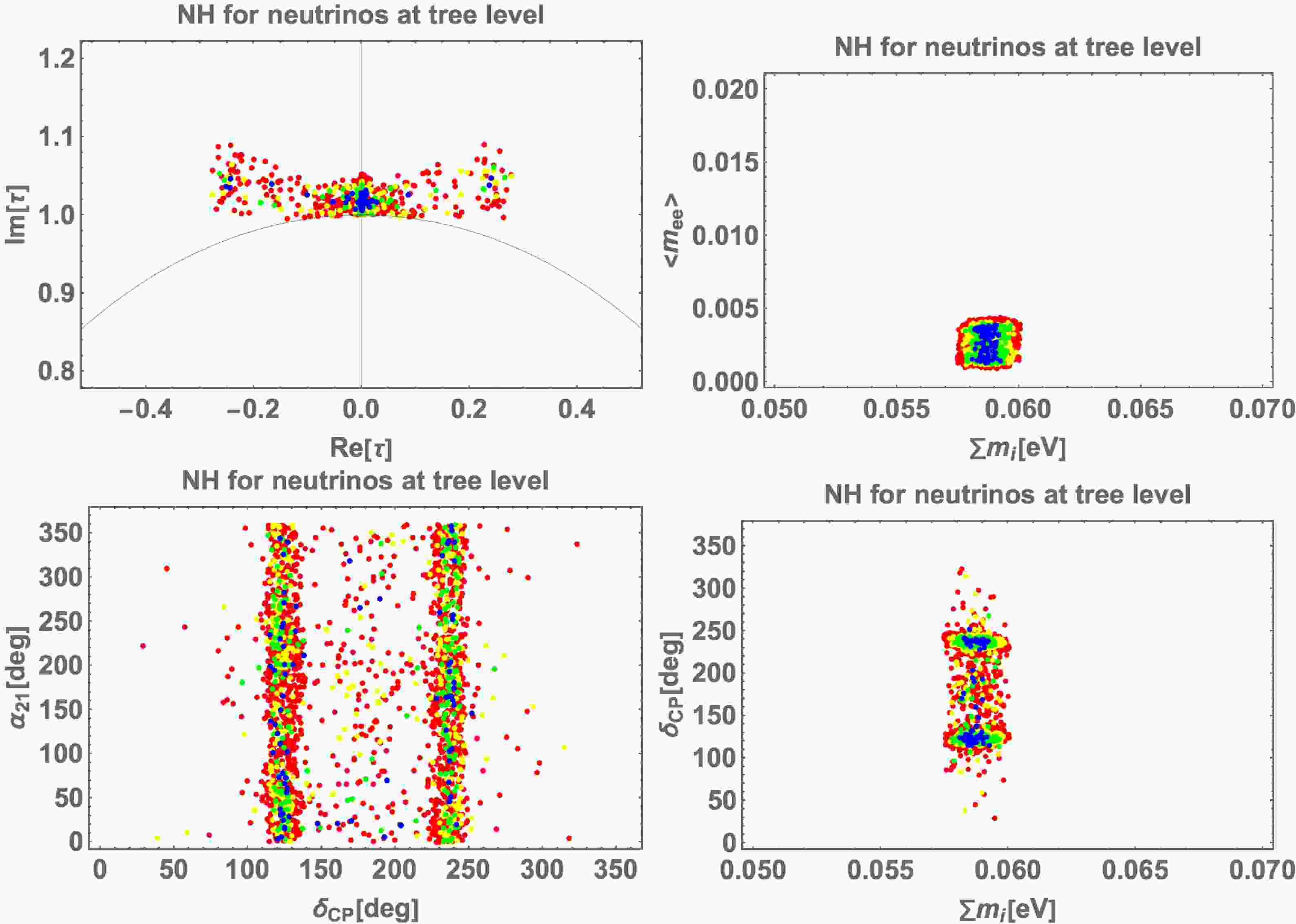
Figure 1 represents NH for the canonical seesaw model. We show an allowed region of τ in the top left panel, $ \langle m_{ee}\rangle $ in terms of sum of neutrino masses $ \sum m_i $ in the top right one, Majorana phase $ \alpha_{21} $ and Dirac CP phase $\delta_{CP}$ in the bottom left one, and Dirac CP phase $\delta_{CP}$ versus sum of neutrino masses $ \sum m_i $ in the bottom right one, respectively. Each color corresponds to the range of $ \Delta\chi^2 $ values such that blue represents$ \Delta\chi^2 \leq 1 $, green represents $ 1< \Delta\chi^2 \le 4 $, yellow represents $ 4< \Delta\chi^2\le 9 $, and red represents $ 9< \Delta\chi^2 \le 25 $. These figures suggest that, within $ 5\sigma $ , 0.058 eV $\lesssim \sum{ m_i }\lesssim $ 0.06 eV, 0.001 ${\rm {eV}}\lesssim\langle m_{ee}\rangle\lesssim 0.004$ eV, any value is possible for $ \alpha_{21} $, and $ \delta_{CP} $ tends to be localized near 120 $ ^\circ $ and 240 $ ^\circ$. As analytically estimated, we have found several solutions near $ \tau=i $.

Figure 1.  (color online) NH for the canonical seesaw model: an allowed region of τ is shown in the top left panel, $ \langle m_{ee}\rangle $ in terms of sum of neutrino masses $ \sum m_i $ in the top right one, Majorana phase $ \alpha_{21} $and Dirac CP phase $ \delta_{CP} $ in the bottom left one, and Dirac CP phase $ \delta_{CP} $ versus sum of neutrino masses $ \sum m_i $ in the bo in the bottom right one, respectively. Each color corresponds to the range of $ \Delta\chi^2 $ values such that blue represents $ \Delta\chi^2 \leq 1 $, green represents $ 1< \Delta\chi^2 \le 4 $, yellow represents $ 4< \Delta\chi^2 \le 9 $, and red represents $ 9< \Delta\chi^2 \le 25 $.

Figure 2 represents IH for the canonical seesaw model, where the legends and colors are the same as those of NH for the canonical seesaw case. These figures suggest that $ 0.098\ {\rm eV}\lesssim\sum m_i\lesssim0.102\ {\rm eV} $, $ \langle m_{ee}\rangle \simeq 0.05 $ eV, $ \alpha_{21} \simeq 0^\circ $, $ 50^\circ\lesssim\delta_{CP}\lesssim130^\circ $, and $ 230^\circ\lesssim\delta_{CP}\lesssim310^\circ $. In our analytical estimation, we have no solutions near $ \tau=i $. However, according to this figure, there would exist solutions near $ \tau=i $. Thus, we investigated the behavior of modular Yukawa functions in terms of τ and found that this function is rather sensitive to deviations from $ \tau=i $.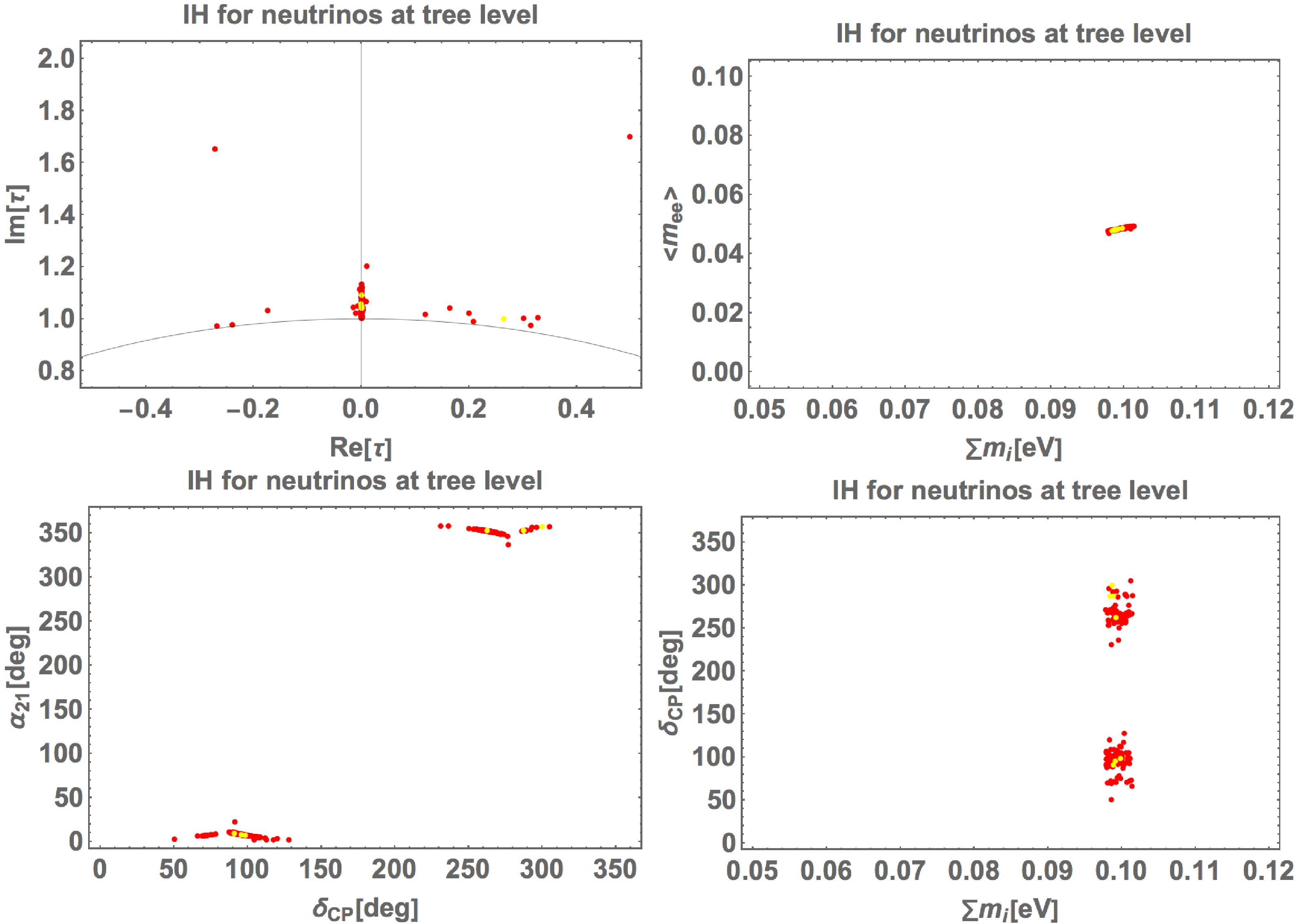

Figure 2.  (color online) IH for the canonical seesaw model; the legends and colors are the same as those of NH for the canonical seesaw case.

Figure 3 represents NH for the radiative seesaw model; the legends and colors are the same as those of NH for the canonical seesaw case. These figures suggest that 0.057 ${\rm eV}\le(\sum m_i,\langle m_{ee}\rangle)\le0.06$ eV, and any values are allowed for phases. In the radiative case, there are solutions near $ \tau=i $ only in case of NH. This is what we expect from our analytical estimation.

Figure 3.  (color online) NH for the radiative seesaw model; the legends and colors are the same as those of NH for the canonical seesaw case.

We studied a double covering of modular $ A_4 $ flavor symmetry in which we constructed lepton models in cases of canonical seesaw and radiative seesaw applying irreducible doublet representations to heavier Majorana fermions that do not have $ A_4 $ symmetry. Then, we have some predictions for both cases except for the IH of radiative seesaw. From our numerical analyses, we conclude the following:

1. In case of NH in the canonical seesaw scenario, within hin $ 5\sigma $, 0.058 ${\rm eV}\lesssim\sum m_i\lesssim0.06$ eV, 0.001 ${\rm eV}\lesssim\langle m_{ee}\rangle\lesssim0.004$ eV, any value is possible for $ \alpha_{21} $, and $ \delta_{CP} $ tends to be localized near 120 $ ^\circ $ and 240 $ ^\circ $.

2. In case of IH in the canonical seesaw scenario, within hin $ 5\sigma $, $ 0.098\ {\rm eV}\lesssim\sum m_i\lesssim0.102\ {\rm eV} $, $ \langle m_{ee}\rangle \simeq 0.05 $ eV, $ \alpha_{21} \simeq 0^\circ $, $ 50^\circ\lesssim\delta_{CP}\lesssim130^\circ $, and $ 230^\circ\lesssim\delta_{CP}\lesssim310^\circ $.

3. In case of NH in the radiative seesaw scenario, within $ 5\sigma $, 0.057 ${\rm eV}\le(\sum m_i,\langle m_{ee}\rangle)\le0.06$ eV, and any values are allowed for phases.

As a future work, it would be interesting to apply this modular symmetry to both the quark and lepton sectors with the common modulus τ. We expect it to result in different predictions from $ A_4 $ modular symmetry due to especially irreducible doublet representations.

In this appendix, we summarize some formulas in the framework of $ T^\prime $ modular symmetry belonging to the $ SL(2,\mathbb{Z}) $ modular symmetry. The $ SL(2,Z_3) $ modular symmetry corresponds to the $ T^\prime $ modular symmetry. The modulus τ transforms as

with $ \{a,b,c,d\} \in Z_3 $ satisfying $ ad-bc=1 $ and $ {\rm Im} [\tau]>0 $. The transformation of modular forms $ f(\tau) $ are given by

where $ f(\tau) $ denotes holomorphic functions of τ with the modular weight k.

In a similar way, the modular transformation of a matter chiral superfield $ \phi^{(I)} $ with the modular weight $ -k_I $ is given by

where $ \rho^{(I)}(\gamma) $ stands for a unitary matrix corresponding to $ T^\prime $ transformation. Note that the superpotential is invariant when the sum of modular weight from fields and modular form is zero and the term is a singlet under the $ T^\prime $ symmetry. It restricts a form of the superpotential, as expressed in Eq. (1).

Modular forms are constructed on the basis of weight 1 modular form, $ Y^{(1)}_2=(Y_1, Y_2)^T $, transforming as a doublet of $ T^\prime $. Their explicit forms are written by the Dedekind eta-function $ \eta(\tau) $ with respect to τ [1, 74]:

Modular forms of higher weight can be obtained from tensor products of $ Y^{(1)}_2 $. We enumerate some modular forms used in our analysis: