


 Abstract
 HTML
HTML Reference
 Related
 PDF
PDF


-
Generally, compact stars are the final stage of the stellar evolution that can be formed because of a radial pressure from core nuclear fusion larger than gravitational forces. There are various gravitational compact objects, including white dwarfs, neutron stars, black holes, and naked singularities. Moreover, compact stars can include more exotic objects, such as strange stars (made of strange quarks) and gravitational condensate stars (non-singular three-layer alternatives to black holes). Such compact objects are usually studied in the General Theory of Relativity (GR), but there are also studies on the modified gravity formalism (for example, on
$ f({\cal{R}}) $ gravity [1–5],$ f({\cal{R}},{\cal{T}}) $ gravity [6–10], teleparallel modified gravity [11, 12], and references therein). Gravity modification can solve many problems of GR, namely dark energy, inflation, and late time accelerated expansion. Apart from presenting new geometrodynamical terms in the Einstein-Hilbert (EH) action integral, we can introduce additional matter fields to solve those problems. In the current study, we modify the GR Lagrangian by using Bose-Einstein Condensate, Kalb-Ramond, and$ U(1) $ gauge fields. -
We address Bose-Einstein condensate as a first additional matter field of our consideration. Bose-Einstein condensate is created from a set of Bose gas particles in the same ground state at very low temperatures, near absolute zero. It is known that Bose-Einstein condensates could be formed from Cold Dark Matter (CDM) axions by thermalization process [13]. It is feasible that such BEC dark matter could recreate galaxy rotational curves. This was shown in [14] with the example of SPARC galactic rotation curves data. Finally, BE condensates could not only act as DM, but also as dark energy. This was shown in [15]. It was also reported by [16] that the Bose-Einstein condensation phase of the boson field could be present in the early universe and could later lead to the formation of dark matter - dark energy unification. Note also that in the aforementioned model, matter density fluctuations are located in the allowed region according to observational data bounds.
Finally, some studies addressed the field of Bose-Einstein condensate stars, generally adopting hydrodynamical representations for the BEC wave function and using polytropic Equation of State. For example, BEC stars were investigated in [17–19].
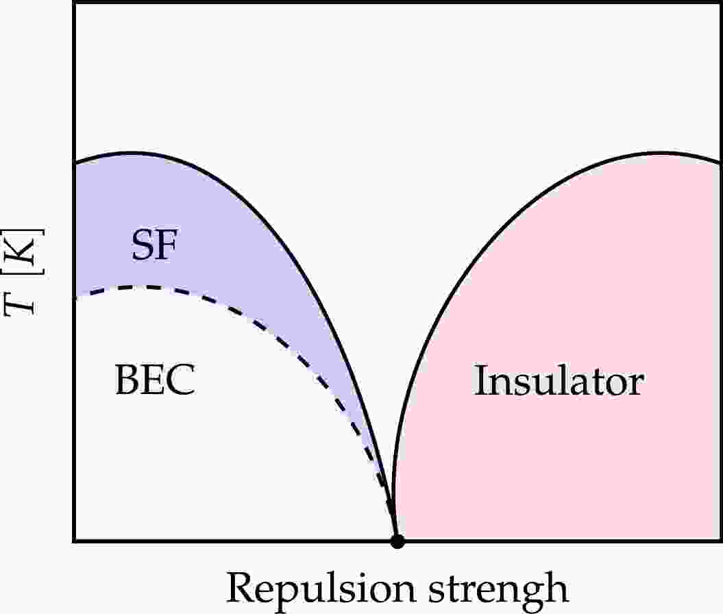
In this paper, we will use an assumption of zero temperature BEC, namely pure BEC, and an assumption of small repulsion strength. Only with these assumptions the Gross–Pitaevskii equation could properly describe the wave function of the Bose-Einstein condensate (for further details, see the phase transition diagram in Fig. 1). There are a couple of phases of Boson fluids in the phase transition diagram. They are related to the different values of temperature T and repulsion strength. Note that fluids with
$ T\gg0 $ and relatively small repulsion strength have superfluid behavior (i.e., vanishing viscosity). However, for smaller values of temperature (assuming that the fluid is in thermodynamical equilibrium), Bose-Einstein condensate could be formed (pure BEC appears at$ T=0 $ ). By contrast, if we assume large values of the repulsion strength, the fluid becomes an insulator.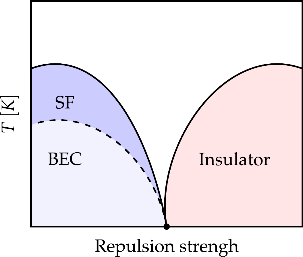
Figure 1. (color online) Phase transition diagram for Boson fluids at low temperature.
-
The second additional matter field is the fully antisymmetric rank-2 tensor field, namely Kalb-Ramond (or B) field. Fields such as Kalb-Ramond is essential in the reproduction of low-energy effective string actions [20]. Moreover, massless KR field could occur in the critical and massless string spectrum due to the compactification to four dimensions [21]. Additionally, this field could be the source of spontaneous Lorentz Symmetry Breaking (LSB) if self-interaction potential and non-vanishing vacuum expectation value (VEV) are assumed [22]. In a pioneering study [23], it was shown that the KR field could be dual to the massive spin-1 field, namely the Proca field. This property could be used in the study of exotic Proca, Boson-Proca stars.
Note also that the KR field could induce cosmological bounce. This was shown in [24] within the modified teleparallel cosmology along with the fact that black holes with KR VEV background behave like Reissner-Nördstrom black holes, despite the absence of charge [25].
-
Gauge field imposing
$ U(1) $ local gauge symmetry (namely photon gauge field) is the third and last exotic matter field that we consider in our study. Stars surrounded by such gauge fields are called gauged boson stars. This type of stars and their shells are widely studied in the literature [26–29]. In this studies, numerical evidence for the existence of gauged boson stars in asymptotically flat/asymptotically AdS spacetimes was provided and it was reported that such solutions, similar to Kerr-Newmann black holes, preserve nonzero electric charge and magnetic dipole momentum [30]. Asymptotically AdS boson stars play an important role in the AdS/CFT (Conformal Field Theory) correspondence. -
This paper is organized as follows. In Section I, we provide a general introduction to the topic of compact (relativistic) objects and their kind into the gravity modification and problems of GR. We also discuss each exotic matter field of our consideration in separated subsections. In Section II, we derive field equations for a perfect fluid stress-energy tensor in terms of Einsteinian gravity and present the formalism used in our study. We also introduce viable Finch-Skea metric potentials. In Section III, we probe Finch-Skea compact stars in the presence of pure Bose-Einstein condensate. In Section IV, we investigate Kalb-Ramond spherically symmetric stellar solutions. In Section V, we study the case with minimal coupling to the gravity gauge field imposing
$ U(1) $ local gauge symmetry. Finally, in Section VI, we provide concluding remarks on the main topics of our study. -
For regular GR gravity, the Einstein-Hilbert action integral reads
$ {\cal{S}}[g,\Gamma,\Psi_i]=\int_{\cal{M}}{\rm d}^4x\sqrt{-g}\frac{1}{2\kappa^2}({\cal{R}}+{\cal{L}}(\Psi_i)), $

(1) where
$ {\cal{R}} $ is the common Ricci scalar curvature,$ g=\det g_{\mu\nu}= \prod^{3}_{\mu,\nu=0}g_{\mu\nu} $ is the determinant of the metric tensor, and κ is the well-known Einstein gravitational constant. Finally, we define$ {\cal{L}}(\Psi_i) $ as a Lagrangian density for additional matter fields$ \Psi_i $ ; Γ is a torsionless metric-affine connection. Varying the aforementioned EH action with respect to the metric tensor inversion$ g^{\mu\nu} $ , we can obtain the set of Einstein Field Equations (EFEs):$ G_{\mu\nu}=\kappa T_{\mu\nu} $

(2) for the case with flat background spacetime. In the equation above,
$ T_{\mu\nu} $ is defined as an stress-energy tensor:$ T_{\mu\nu} = -\frac{2}{\sqrt{-g}}\frac{\delta(\sqrt{-g}{\cal{L}}(\Psi_i))}{\delta g^{\mu\nu}}. $

(3) In this study, the stress-energy-momentum tensor is assumed to be anisotropic and corresponding to a perfect fluid. Thus,
$ T_{\mu}^{\nu} = (\rho+p_t)U_\mu U^\nu - p_t\delta^\nu_\mu + (p_r-p_t)V_\mu V^\nu . $

(4) Here, as usual, ρ denotes the energy density;
$ p_r $ and$ p_t $ are the radial and tangential pressures, respectively;$ U_\mu $ is normalized by$ U^\mu U_\mu=-1 $ timelike four-velocity; and$ V_\mu $ is a spacelike (radial) four-vector.Let us consider a spherically symmetric line element with metric signature
$ (+;-;-;-) $ :$ {\rm d}s^2 ={\rm e}^{\nu(r)}{\rm d}t^2-{\rm e}^{\lambda(r)}{\rm d}r^2-r^2{\rm d}\Omega^2_{D-2}, $

(5) where
${\rm e}^{\nu(r)}$ and${\rm e}^{\lambda(r)}$ are metric potentials, and${\rm d}\Omega^2_{D-2}$ is the$ D-2 $ dimensional unit sphere line element:$ \begin{aligned}[b] {\rm d}\Omega^2_{D-2}=&{\rm d}\theta_1^2+\sin^2\theta_1{\rm d}\theta_2^2+\sin^2\theta_1\sin^2\theta_2{\rm d}\theta_3^2+...\\&+\bigg(\prod^{D-3}_{j=1}\sin^2\theta_j\bigg){\rm d}\theta^2_{D-2} . \end{aligned} $

(6) Next, we restrict our analysis to
$ D=(3+1) $ dimensions. Accordingly, the stress-energy-momentum tensor components are [31]$ \kappa \rho=\frac{1-{\rm e}^{-\lambda(r)}}{r^2}+\frac{{\rm e}^{-\lambda(r)}\lambda'(r)}{r}, $

(7) $ \kappa p_r=\frac{{\rm e}^{-\lambda(r)}-1}{r^2}+\frac{{\rm e}^{-\lambda(r)}\nu'(r)}{r}, $

(8) $ \kappa p_t = {\rm e}^{-\lambda}\left(\frac{\nu''(r)}{2}+\frac{\nu'(r)^2}{4}-\frac{\nu'(r)\lambda'(r)}{4}+\frac{\nu'(r)-\lambda'(r)}{2r}\right). $

(9) -
Throughout the present paper, we consider that our compact star solution imposes Finch-Skea symmetry and is physically viable, resulting in non-singular metric potentials [32]:
$ {\rm e}^{\nu(r)}=\left(A+\frac{1}{2}Br\sqrt{r^2C}\right)^2, $

(10) $ {\rm e}^{\lambda(r)}=\left(1+Cr^2\right), $

(11) where A, B, and C have constant values and are called Finch-Skea coefficients. Using the Finch-Skea ansatz above, we can rewrite the field equations:
$ \kappa \rho=\frac{C \left(C r^2+3\right)}{\left(C r^2+1\right)^2}, $

(12) $ \kappa p_r=-\frac{C \left(2 A \sqrt{C r^2}+B r \left(C r^2-4\right)\right)}{\left(C r^2+1\right) \left(2 A \sqrt{C r^2}+B C r^3\right)}, $

(13) $ \kappa p_t = \frac{C \left(B r \left(C r^2+4\right)-2 A \sqrt{C r^2}\right)}{\left(C r^2+1\right)^2 \left(2 A \sqrt{C r^2}+B C r^3\right)}. $

(14) In the following subsection, we derive exact solutions for the Finch-Skea coefficients using junction conditions at the boundary.
-
Extra matching conditions for spherically symmetric relativistic objects were provided by Goswami et al. [33], and it was shown that constraints on the thermodynamic properties and stellar structure are purely mathematical [34]. For spacetime with axymptotically flat background, the exterior region can be considered as a Schwarzschild’s spacetime:
$ {\rm d}s^2 = \bigg(1-\frac{2M}{r}\bigg){\rm d}t^2 - \bigg(1-\frac{2M}{r}\bigg)^{-1}{\rm d}r^2 - r^2 {\rm d}\theta^2 - r^2 \sin^2 \theta {\rm d}\phi^2 ,$

(15) where M indicates total gravastar mass. The above line element implies conditions of metric potential continuity at the boundary:
$ {\rm{Continuity\;of}}\;g_{tt}:\quad 1-\frac{2M}{R}={\rm e}^{\nu(r)}, $

(16) $ {\rm{Continuity\;of}}\;\frac{\partial g_{tt}}{\partial r}:~ \frac{2M}{R^2}=-B \left(2 A \sqrt{C R^2}+B C R^3\right), $

(17) $ {\rm{Continuity\;of}}\;g_{rr}:\quad \bigg(1-\frac{2M}{R}\bigg)^{-1}={\rm e}^{\lambda(r)}, $

(18) $ {\rm{Vacuum\;condition}}:\quad p\rvert_{r=R}=0. $

(19) The solutions for the above continuity conditions are as follows:
$ A=\frac{3 M-2 R}{2 \sqrt{R} \sqrt{R-2 M}}, $

(20) $ B=\frac{\sqrt{\dfrac{M}{R-2 M}} \sqrt{R-2 M}}{\sqrt{2} R^{3/2}}, $

(21) $ C=\frac{2 M}{R^2 (R-2 M)}. $

(22) Plots of metric potentials using the junction conditions defined above are depicted in Fig. 2 for relativistic star PSRJ1416-2230, which has a mass
$ M+1.97 $ and radius$ R=9.69 $ . We can now proceed further and define a Bose-Einstein condensate (BEC) field minimally coupled to gravity.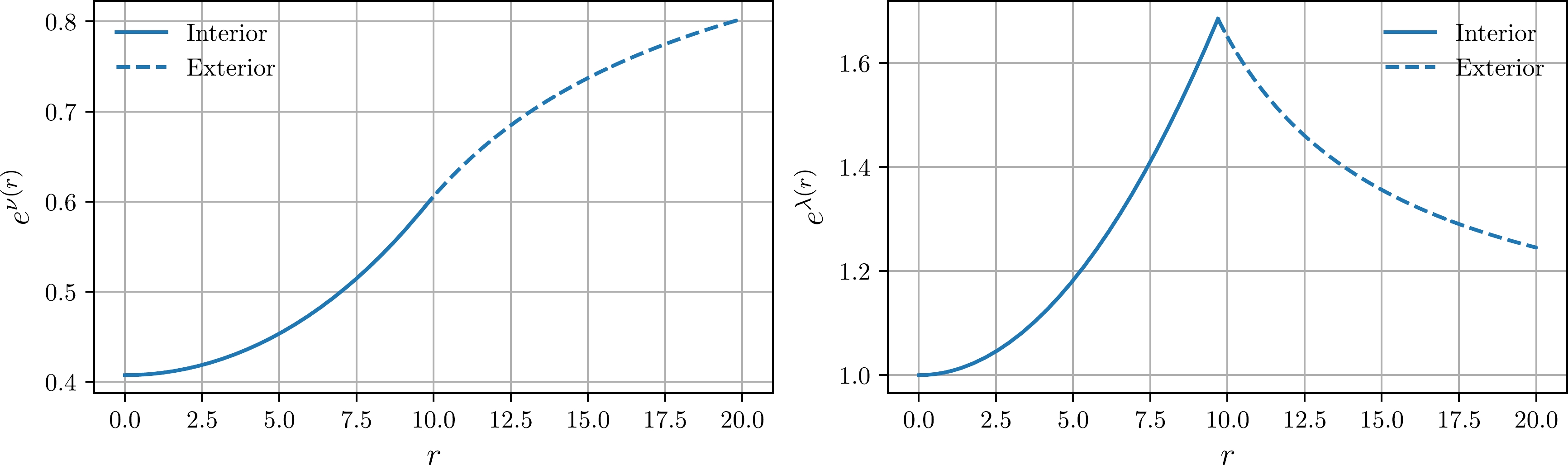
Figure 2. (color online) Finch-Skea interior and exterior metric potentials with adopted junction conditions for compact star PSRJ1416-2230.
-
Generally, the ground state of Bose-Einstein condensate can be described by a complex scalar field [35]. If we assume minimal coupling to an Einsteinian gravity Bose-Einstein field, the classical GR Lagrangian (1) transforms as follows:
$ {\cal{S}}[g,\Gamma,\Psi_i,\hat{\phi}]=\int_{\cal{M}}{\rm d}^4x\sqrt{-g}\frac{1}{2\kappa^2}({\cal{R}}+{\cal{L}}(\Psi_i)+{\cal{L}}(\hat{\phi})), $

(23) where we define [36]
$ {\cal{L}}(\hat{\phi})=-g_{\mu\nu}\nabla^\mu\hat{\phi}^\dagger \nabla^\nu \hat{\phi}-m^2\hat{\rho}-U(\hat{\rho}). $

(24) Here, evidently,
$ \hat{\phi} $ is a Bose-Einstein field,$ \hat{\phi}^\dagger $ is its complex conjugate,$ m^2 $ is a scalar Bose field mass, and finally,$ U(\hat{\rho}) $ is the so-called self-interaction potential, which can be expanded in a series with many-body interaction terms (external potential$ V(\hat{\rho}) $ for absent Bose field) [37, 38]:$ U(\hat{\rho})=\frac{\lambda_2}{2}\hat{\rho}^2+\frac{\lambda_3}{6}\hat{\rho}^3+...-\frac{\lambda_2}{8}T^2\hat{\rho}+\frac{\pi^2}{90}T^4\hat{\rho}^2 , $

(25) where the first term corresponds to the regular two particle interaction, and
$ \rho=\hat{\phi}^\dagger\hat{\phi} $ is the Bose field probability density. For the sake of simplicity, in the definition of self-interaction potential, we will use only the terms up to the quadratic one. Therefore, we redefine the set of self-interaction coupling coefficients to η. We also assume that our Bose-Einstein condensate is pure, and therefore,$ T=0 $ . Using (3), we can easily obtain the stress-energy tensor for our Bose field:$ \begin{gathered} T_{\mu\nu}^{\hat{\phi}}=\nabla_\mu \hat{\phi}^\dagger \nabla_\nu \hat{\phi}+\nabla_\mu \hat{\phi}\nabla_\nu \hat{\phi}^\dagger -g_{\mu\nu}\Big(g^{\alpha\beta}\nabla_\alpha \hat{\phi}^\dagger \nabla_\beta \hat{\phi} +m^2\hat{\rho}+U(\hat{\rho})\Big). \end{gathered} $

(26) Given that we are working with a scalar field, for the first order covariant derivatives further we imply the proper transformation
$ \nabla_\mu \hat{\phi}\to \partial_\mu \hat{\phi} $ . To numerically derive the Bose field, it is also useful to introduce modified massive Klein-Gordon equation:$ g_{\mu\nu}\nabla^\mu \nabla^\nu \hat{\phi}-\bigg(m^2+U'(\hat{\rho})\bigg)\hat{\phi}=0. $

(27) Using the assumption of harmonic time dependence, we can impose the transformation
$ \hat{\phi}=\exp(-{\rm i}\omega t)\phi(r), $

(28) where
$ \phi(r) $ is a real function that depends only on the radial coordinate r, and therefore$ \hat{\rho}=\hat{\phi}\hat{\phi}^\dagger=\phi^2 $ . Using the aforementioned assumption, the Klein-Gordon equation reduces to a Gross–Pitaevskii–like equation [39]:$ {\rm i}\hslash \nabla_t \hat{\phi}=\Bigg(-\frac{\hslash^2}{2m}\nabla^i\nabla_i+\underbrace{mV_{{\rm{ext}}}}_{\rm{0}}+\eta\hat{\rho}^2\Bigg)\hat{\phi}, $

(29) where
$ \nabla_i\hat{\phi} = \frac{1}{\sqrt{-g}}\partial_i(\sqrt{-g}g^{ij}\partial_i\hat{\phi}) $

(30) and
$ V_{{\rm{ext}}} $ is a external integral. We solved the equation above numerically for the set of initial conditions$ \phi(0)= 10 $ and$ \phi'(0)=C $ . Solutions for the above equation have a viable behavior for$ \omega\gg|\eta|\land m $ and for relatively small values of these parameters. The oscillating solution for$ \phi(r) $ is presented in Fig. 3.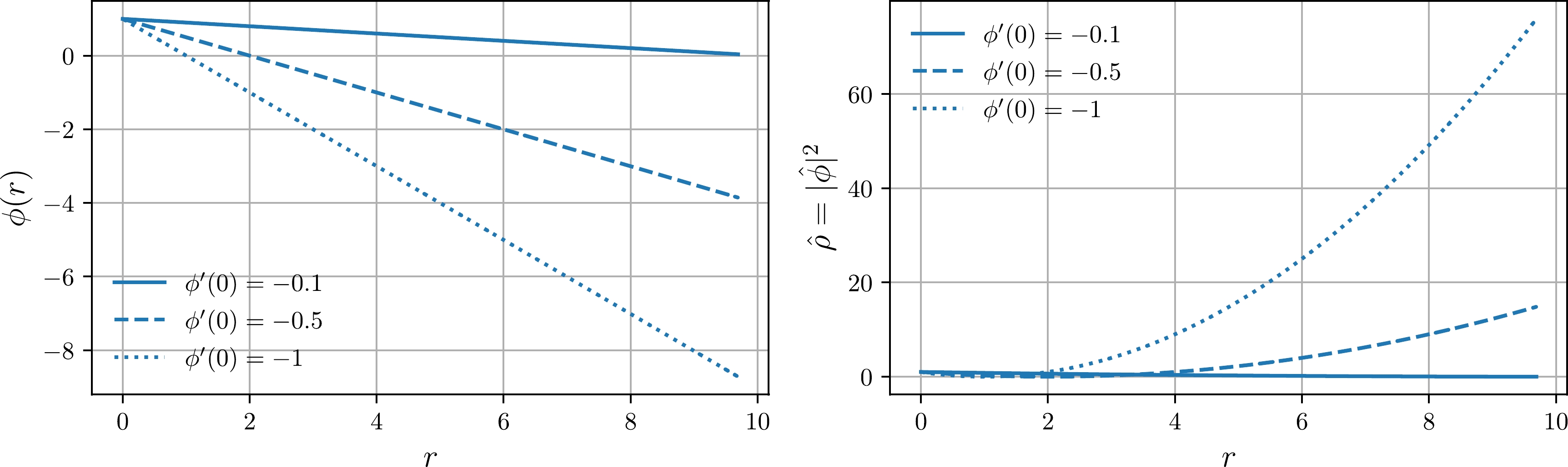
Figure 3. (color online) (left plot) Solutions for the scalar field
$ \phi(r) $ governed by Gross–Pitaevskii equation; (right plot) probability density for Bose-Einstein condensate. To obtain these solutions, we set$ m=\eta=10^{-8} $ ,$ \omega=10^{-2} $ . The mass and radius were similar to those of compact star PSRJ1416-2230 ($ M=1.97 $ and$ R=9.69 $ ).Finally, we can derive field equations from the modified Einstein-Hilbert action (44):
$ \kappa (\rho+\rho^{\hat{\phi}})=\frac{1-{\rm e}^{-\lambda(r)}}{r^2}+\frac{{\rm e}^{-\lambda(r)}\lambda'(r)}{r}, $

(31) $ \kappa (p_r+p_r^{\hat{\phi}})=\frac{{\rm e}^{-\lambda(r)}-1}{r^2}+\frac{{\rm e}^{-\lambda(r)}\nu'(r)}{r}, $

(32) $ \begin{aligned}[b]\kappa (p_t+p_t^{\hat{\phi}}) = {\rm e}^{-\lambda}\Bigg(\frac{\nu''(r)}{2}+\frac{\nu'(r)^2}{4}-\frac{\nu'(r)\lambda'(r)}{4}+\frac{\nu'(r)-\lambda'(r)}{2r}\Bigg),\end{aligned} $

(33) where [40]
$ \rho^{\hat{\phi}} = -{\rm e}^{-\nu}\omega^2\phi^2 - {\rm e}^{-\lambda}(\phi')^2 + V(\phi), $

(34) $ p_r^{\hat{\phi}} = -{\rm e}^{-\nu}\omega^2\phi^2 - {\rm e}^{-\lambda}(\phi')^2 - V(\phi), $

(35) $ p_t^{\hat{\phi}} = -{\rm e}^{-\nu}\omega^2\phi^2 + {\rm e}^{-\lambda}(\phi')^2 - V(\phi). $

(36) Here, we define
$ V(\Phi)=m^2\hat{\rho}^2/2+U(\hat{\rho}) $ . In the next subsection, we probe the behavior of a Finch-Skea star minimally coupled to Bose-Einstein condensate. -
Energy conditions are probes of relativistic model viability. Generally, there exist four energy conditions, namely Weak Energy Condition (WEC), Null Energy Condition (NEC), Strong Energy Condition (SEC), and Dominant Energy Condition (DEC). For a model to be physically plausible, all of the aforementioned energy conditions must be satisfied at the every point of the manifold. ECs derived from temporal Raychaudhuri equations are defined as follows:
● Null Energy Condition (NEC):
$ \rho +p_{r}\geq 0 $ and$\rho +p_{t}\geq 0;$ ● Weak Energy Condition (WEC)
$ \rho >0 $ and$ \rho +p_{r}\geq 0 $ and$\rho +p_{t}\geq 0;$ ● Dominant Energy Condition (DEC):
$ \rho -|p_{r}|\geq 0 $ and$\rho -|p_{t}|\geq 0;$ ● Strong Energy Condition (SEC):
$\rho +p_{r}+2p_{t}\geq 0;$ Energy conditions for Finch-Skea PSRJ1416-2230 star minimally coupled to Bose-Einstein condensate are depicted in Fig. 4. Note that NEC is validated for tangential and radial pressures, DEC is validated for both pressure types, and SEC is obeyed everywhere. Note also that Null, Dominant, and Strong Energy Conditions will be still satisfied for relatively small and positive values of Bose field mass squared, frequency, and self-coupling constant η.
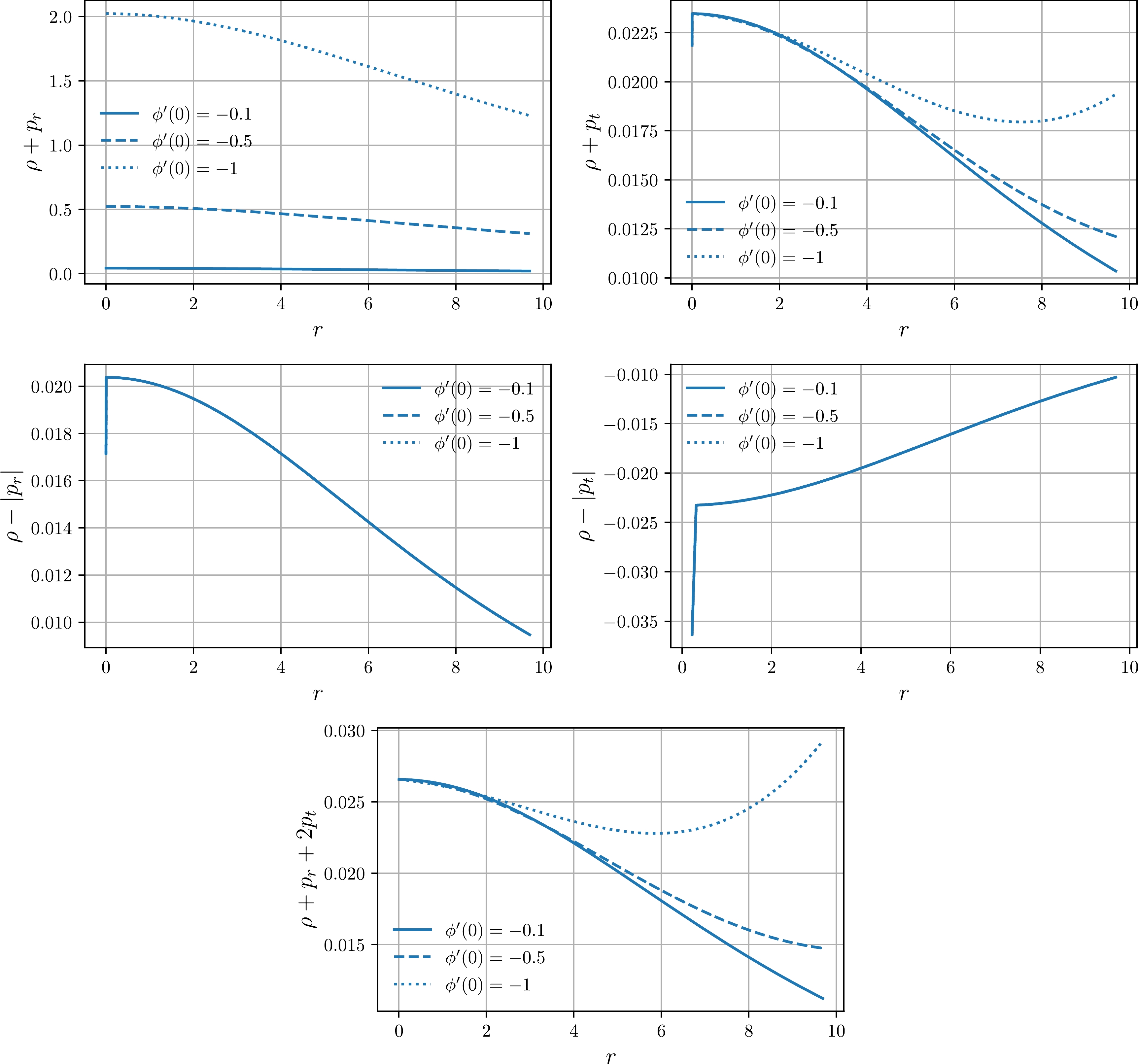
Figure 4. (color online) Null, Dominant, and Strong energy conditions for Finch-Skea PSRJ1416-2230 star minimally coupled to Bose-Einstein condensate (we set
$ m=\eta=10^{-8} $ ,$ \omega=10^{-2} $ ). -
To probe the nature of matter content in the Finch-Skea star interior region, we use the Equation of State (EoS) parameter, which is defined as
$ \omega_r=p_r/\rho,\quad \omega_t=p_t/\rho. $

(37) We can depict the energy density and anisotropic pressure gradients by simply calculating
$ \rho'(r) $ and$ p_r'(r) $ ,$ p_t'(r) $ . EoS and stress-energy tensor component gradients are shown in Fig. 5. Note that, at the stellar origin, radial EoS is asymptotically ($ \phi'(0)\to-\infty $ ) described by a stiff Zeldovich fluid and tangentially described by a dark-energy fluid. However, for all negative values of$ \phi'(0) $ , the initial condition radial fluid is a regular one in the bounds$ \omega\in(0,1) $ and tangential is quintessence in the bounds$ \omega\in(-1,0) $ . Besides, the gradients of energy density and anisotropic pressures can have both positive and negative values in the stellar interior. However, generally because of the asymptotical flatness, gradients vanish at the region$ r\to \infty $ .
Figure 5. (color online) (left plot) Equation of State for radial and tangential pressures (parameter values are the same as those for ECs); (right plot) gradient of the energy density and anisotropic pressures.
-
Stability of the matter content in the stellar interior can be investigated using the well known Tolman-Oppenheimer-Volkoff equilibrium condition, which is expressed in its modified form as follows [41–44]:
$ -\frac{{\rm d}p_{r}}{{\rm d}r}-\frac{\nu'(r)}{2}(\rho+p_{r})+\frac{2}{r}(p_{t}-p_{r})+F_{\rm{ex}}=0 . $

(38) It is evident that, in the modified form of the TOV equilibrium condition, there is one extra force, namely
$ F_{\rm{ex}} $ , which is present because of the stress-energy-momentum tensor discontinuity ($ \nabla^\mu T_{\mu\nu}\neq0 $ ) to ensure stability of the relativistic object. In classical and modified TOVs, three additional forces are present: hydrodynamical$ F_{\rm{H}} $ , gravitational$ F_{\rm{G}} $ , and anisotropic$ F_{\rm{A}} $ :$ F_{\rm H}=-\frac{{\rm d}p_{r}}{{\rm d}r},\;\;\;\;\;\;\;F_{\rm A}=\frac{2}{r}(p_{t}-p_{r}), \;\;\;\;\;\;\; F_{\rm G}=-\frac{\nu^{'}}{2}(\rho+p_{r}), $

(39) and therefore, we can easily rewrite MTOV (42) as follows:
$ F_{\rm A}+F_{\rm G}+F_{\rm H}+F_{\rm ex}=0 .$

(40) The solutions for each force present in MTOV are depicted in Fig. 6. Note that both the hydrodynamical force
$F_{\rm H}$ and extra force$F_{\rm ex}$ have positive values in the whole interior radial domain, and the gravitational and anisotropic forces are always negative and vanish asymptotically. Hence, for the Finch-Skea star in the presence of Bose-Einstein condensate, modified TOV equilibrium is satisfied (relativistic star is stable) if an extra force is present.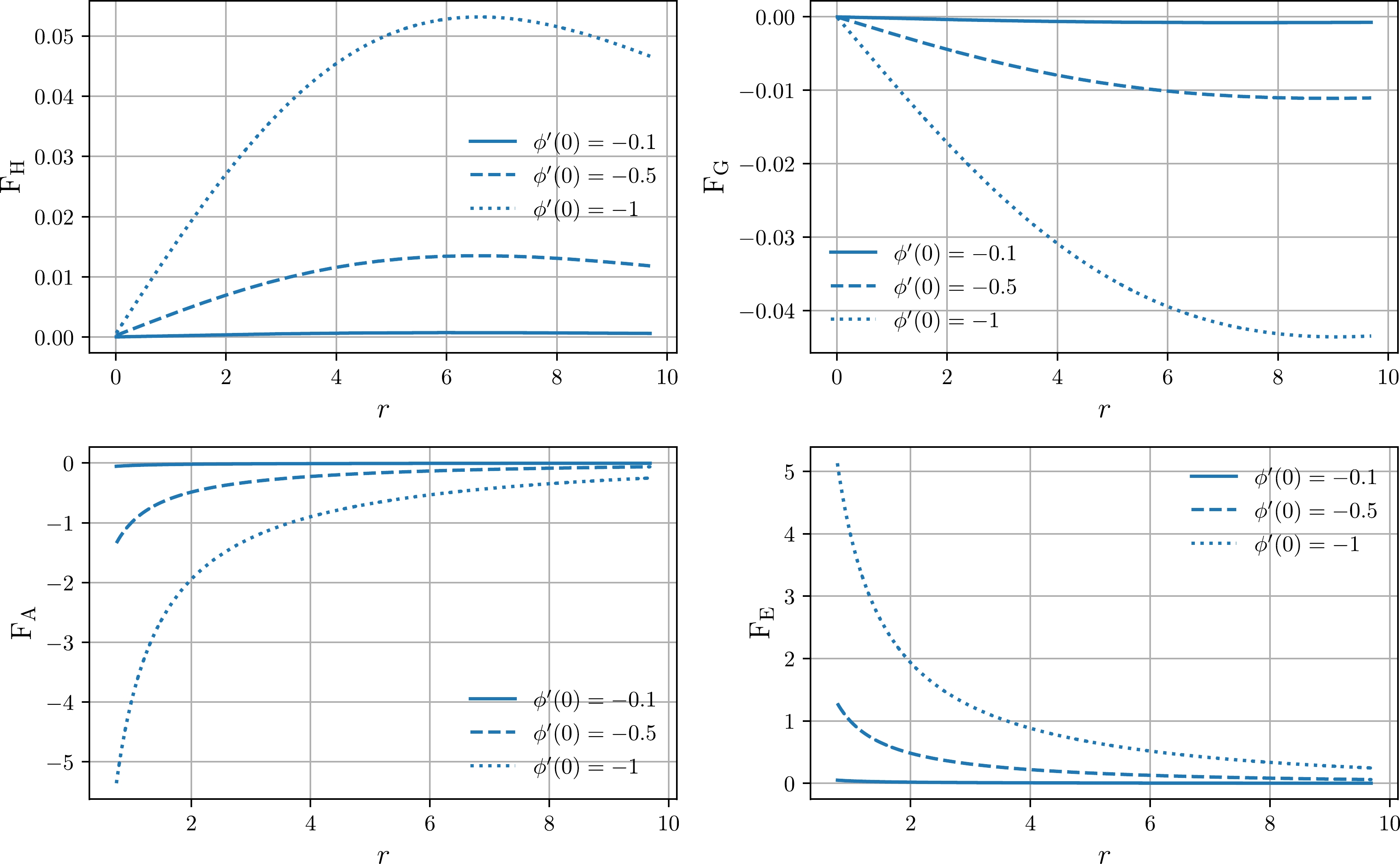
Figure 6. (color online) Modified TOV forces for Finch-Skea star minimally coupled to Bose-Einstein condensate.
-
Adiabatic index is a tool that can be used to probe relativistic objects via adiabatic perturbations. It was first introduced in a study by Chandrasekhar [45], who predicted that, for a relativistic system to be stable, the adiabatic index should exceed
$ 4/3 $ . This adiabatic index is defined as follows [46]:$ \Gamma = \frac{p_r+\rho}{p_r}\frac{{\rm d}p_r}{{\rm d}\rho}. $

(41) Adiabatic index solutions are plotted in Fig. 7. Generally, for the same values of parameters used in the energy conditions subsection, Γ constraint is satisfied at the area near origin and envelope for small
$ \phi'(0)<0 $ and satisfied everywhere for$ \phi'(0)\ll0 $ . Moreover, stability holds for relatively small and positive values of ω, η, and m.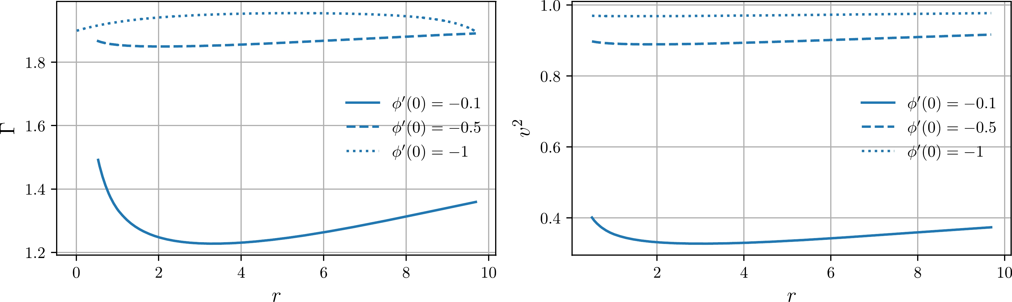
Figure 7. (color online) (first row) Adiabatic index for Finch-Skea star minimally coupled to Bose-Einstein condensate; (second row) speed of sound for Finch-Skea star minimally coupled to Bose-Einstein condensate.
-
Finally, we can also define surface redshift:
$ {\cal{Z}}_s = |g_{tt}|^{-1/2}-1 . $

(42) For anisotropic matter distribution, this redshift must not exceed the value of 2. Numerical solutions for surface redshift for different compact stars are depicted in Fig. 8. According to the plotted data, we can conclude that our solution satisfies the surface gravitational redshift constraint.
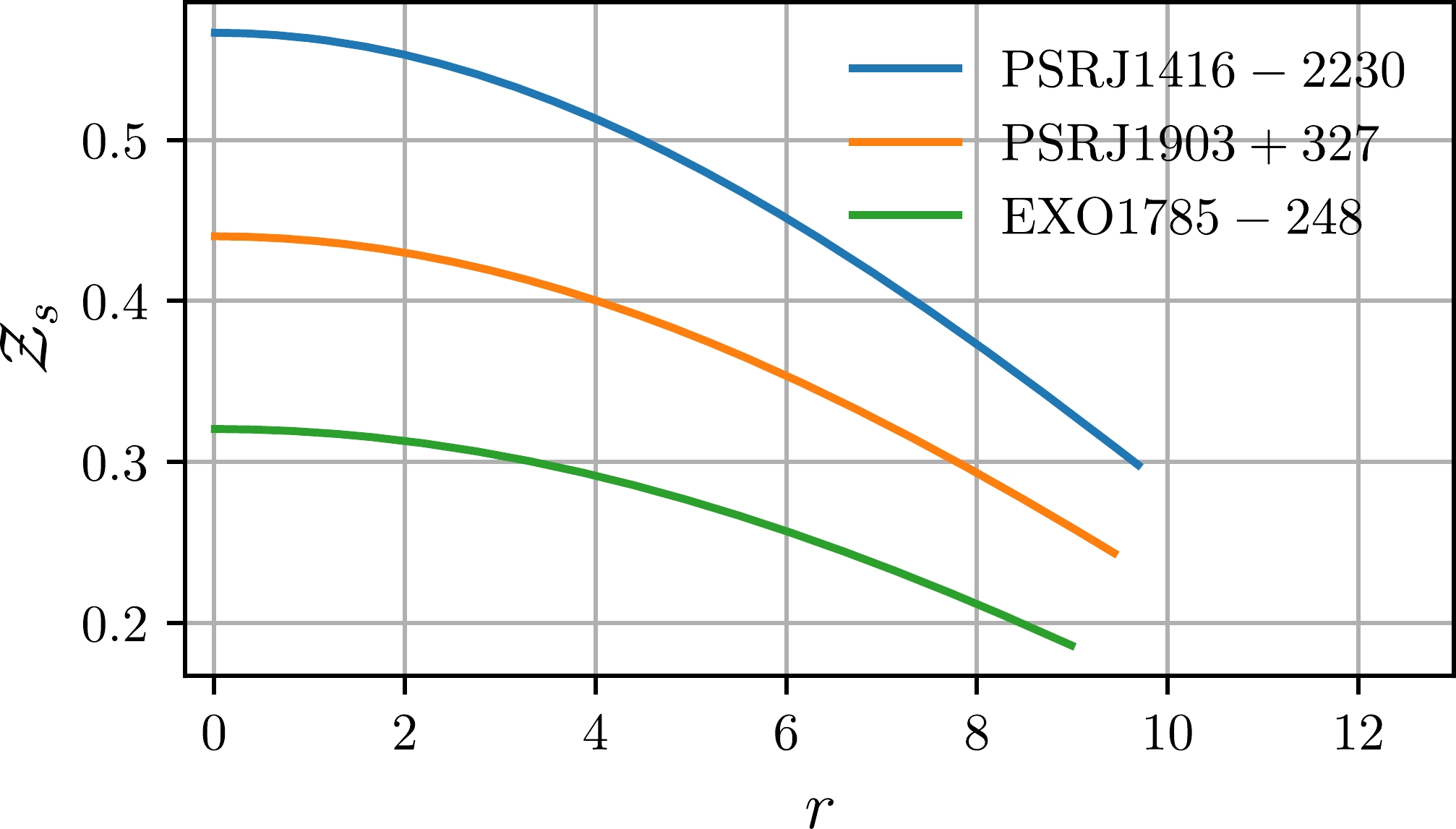
Figure 8. (color online) Surface (gravitational) redshift for Finch-Skea stellar interior (parameter values are the same as those for ECs).
-
Another important criterion of matter content viability is the so-called speed of sound. This quantity is defined in the following way (derived from ultra-relativistic hydrodynamics):
$ v^2 = \frac{{\rm d}p_r}{{\rm d}\rho}\leq c^2 =1. $

(43) The inequality above needs to be satisfied in order to respect causality constraints. A solution for the speed of sound is provided in the third plot of Fig. 7. Note that inequality
$ v^2\leq c^2 $ always holds, which is a necessary condition. It is also important to observe that asymptotically$ \phi'(0)\to-\infty $ , our fluid becomes massless, given that$ v^2=c^2 $ . At this point, we have already probed all the necessary parameters for minimally coupled Bose-Einstein condensate and can proceed with the minimally coupled Kalb-Ramond field case. -
In this section, we investigate the compact stars admitting Finch-Skea symmetry in the presence of background Kalb-Ramond (KB) field. For this particular case, the total Einstein-Hilbert action integral is expressed as follows:
$\begin{aligned}[b] {\cal{S}}[g,\Gamma,\Psi_i,\hat{\phi},B_{\mu\nu}]=&\int_{\cal{M}}{\rm d}^4x\sqrt{-g}\frac{1}{2\kappa^2}\big({\cal{R}}+{\cal{L}}(\Psi_i)\big)\\&+\int_{\cal{M}}{\rm d}^4x\sqrt{-g} H_{\mu\nu\alpha}H^{\mu\nu\alpha}. \end{aligned} $

(44) In the action above,
$ H_{\mu\nu\alpha} $ is defined as the Kalb-Ramond field strength:$ H_{\mu\nu\alpha}=\partial _\mu B_{\nu\alpha}+\partial _\nu B_{\alpha\mu}+\partial _\alpha B_{\mu\nu}, $

(45) where
$ B_{\mu\nu} $ is the antisymmetric rank 2 tensor, namely the Kalb-Ramond field. For the KB field, we have a set of two EoMs expressed as follows [47–49]:$ \frac{1}{\sqrt{-g}}\partial_\mu (\sqrt{-g}H^{\mu\nu\alpha})=0, $

(46) $ \epsilon^{\mu\nu\alpha\beta}\partial_\mu (\sqrt{-g}H_{\nu\alpha\beta}). $

(47) Here,
$ \epsilon^{\mu\nu\alpha\beta} $ is the well known Levi-Cevita symbol, which, for Minkowskian spacetime, is equal to unity if its indices are an even permutation of$ (1234) $ , is equal to$ -1 $ if its indices are an odd permutation of$ (1234) $ , and vanishes if one of the indices repeats. For the KB field, the stress-energy-momentum tensor reads [50]$ T^{\mu\nu}_B=\frac{1}{2}H^{\alpha\beta\mu}H^{\nu}_{\;\alpha\beta}-\frac{1}{2}g^{\mu\nu}H^{\alpha\beta\gamma}H_{\alpha\beta\gamma}, $

(48) where we consider that there is no external potential present. Solving field equation (46), we can obtain the solution for the Kalb-Ramond field strength [24]:
$ H_{\mu\nu\alpha}=\epsilon^{\mu\nu\alpha\beta}\partial_\beta \phi . $

(49) Here, ϕ is a real scalar field whose evolution is governed by the following equation:
$ \nabla_\mu\nabla^\mu\phi =0 . $

(50) This is exactly a massless wave equation. As usual, we assumed only radial coordinate dependence for real scalar fields and used the following set of initial conditions to solve the wave equation above numerically:
$ \phi(0)=0.1 $ and$ \phi'(0)=C $ (if we assume that the radial derivative of a scalar field vanishes at the origin, the scalar field will have a constant solution). To numerically plot the results in the presence of the KB field, we varied the values of the scalar field first order radial derivative at the origin$ \phi'(0) $ . Finally, using the previously defined stress-energy-momentum tensor for the KB field, we can derive a new set of (modified) Einstein Field Equations:$ \begin{gathered} \rho= {\rm e}^{\lambda (r)-4 \nu (r)} \phi '(r)^2-\frac{{\rm e}^{-\lambda (r)} \left(r \lambda '(r)+{\rm e}^{\lambda (r)}-1\right)}{r^2}, \end{gathered} $

(51) $ \begin{gathered} p_r =-\frac{{\rm e}^{-\lambda (r)} \left(r \nu '(r)+1\right)}{r^2}+\frac{1}{r^2}+3 {\rm e}^{-3 \lambda (r)} \phi '(r)^2 , \end{gathered} $

(52) $ \begin{aligned}[b] p_t =&\frac{{\rm e}^{-\lambda (r)} \left(\left(r \nu '(r)+2\right) \left(\lambda '(r)-\nu '(r)\right)-2 r \nu ''(r)\right)}{4 r}-\frac{{\rm e}^{\lambda (r)} \phi '(r)^2}{r^8} . \end{aligned} $

(53) Given that our spacetime admits spherical symmetry, without loss of generality, we can work only in the equatorial plane adopting
$ \theta=\pi/2 $ . -
Energy conditions for Finch-Skea star minimally coupled to the Kalb-Ramond field are illustrated in Fig. 9. It is evident from these data that all the energy conditions are violated. These conditions could be satisfied if we set other values of free parameters ω and initial conditions
$ \phi(0) $ and$ \phi'(0) $ , but in that case, the speed of sound would exceed$ c^2 $ , which is forbidden.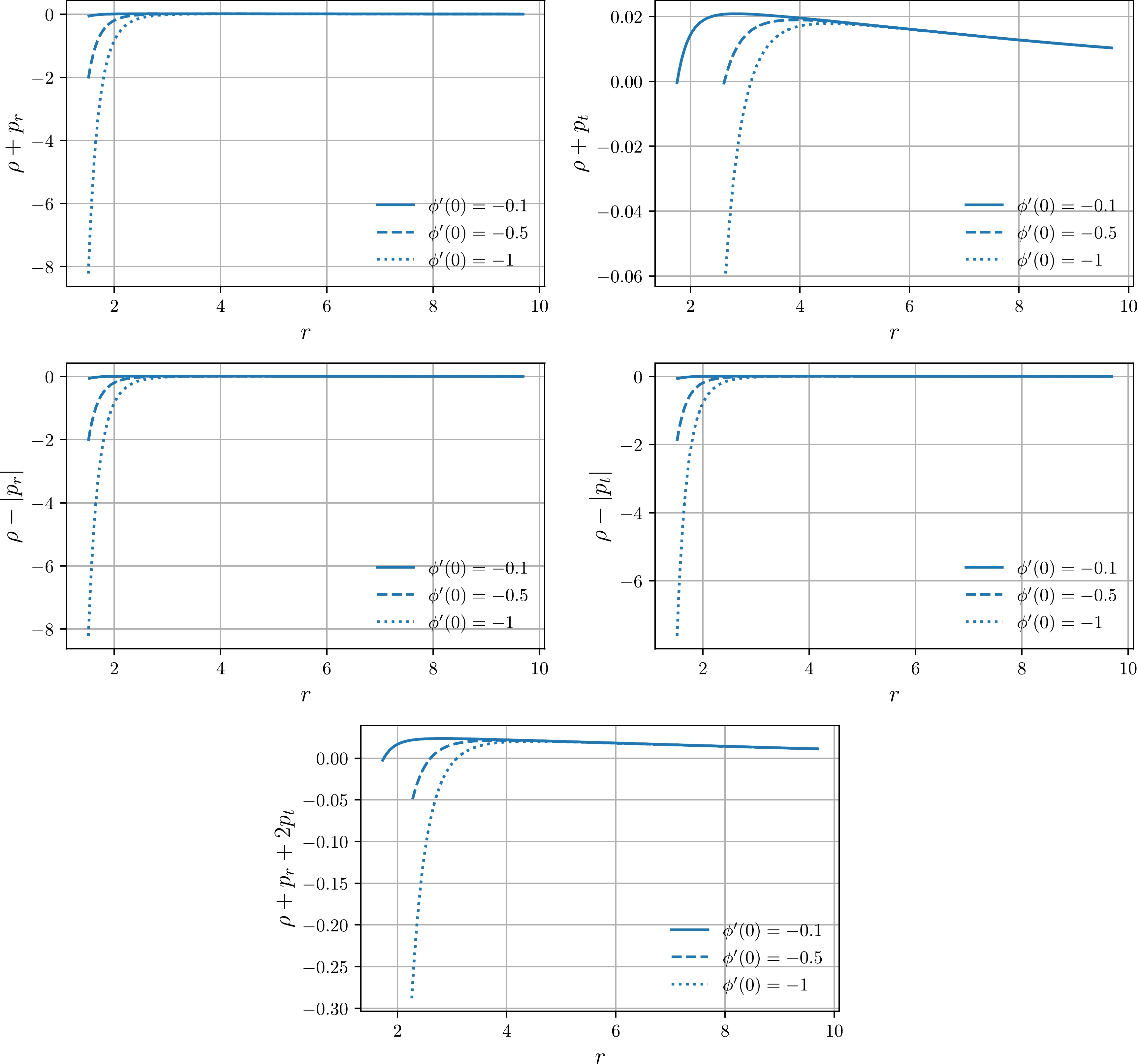
Figure 9. (color online) Null, Dominant, and Strong energy conditions for Finch-Skea PSRJ1416-2230 star minimally coupled to Kalb-Ramond field.
-
In addition to the energy conditions, we also probed the equation of state for our stellar matter content and energy density, as well as anisotropic pressure radial derivatives behavior. The results are plotted in Fig. 10. EoS has regular behavior (
$ 0<\omega<1 $ ) for radial pressure and is negative (quintessence) for tangential pressure (near the stellar core), regular near envelope. Finally, gradients are generally positive for energy density and radial pressure, whereas they are negative for tangential pressure.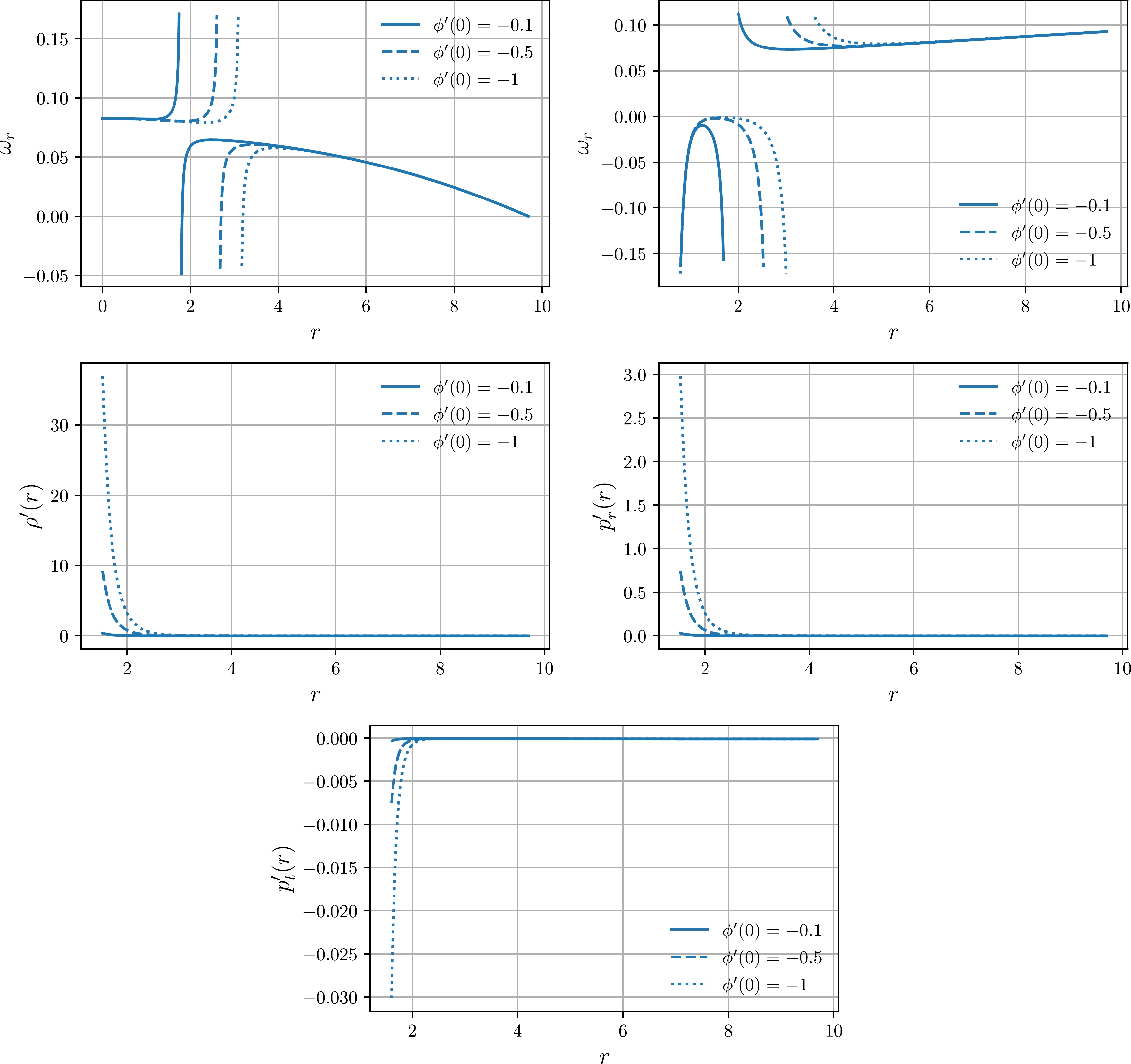
Figure 10. (color online) Equation of state and radial derivative of stress-energy tensor components for Finch-Skea star coupled to KB field.
-
It is also convenient to investigate the TOV stability of our Finch-Skea stellar solution coupled to the KB field. Graphical results of such investigation are provided through the four plots shown in Fig. 11. Note that only the hydrodynamical force has negative values; gravitational, anisotropic, and extra forces have positive values.
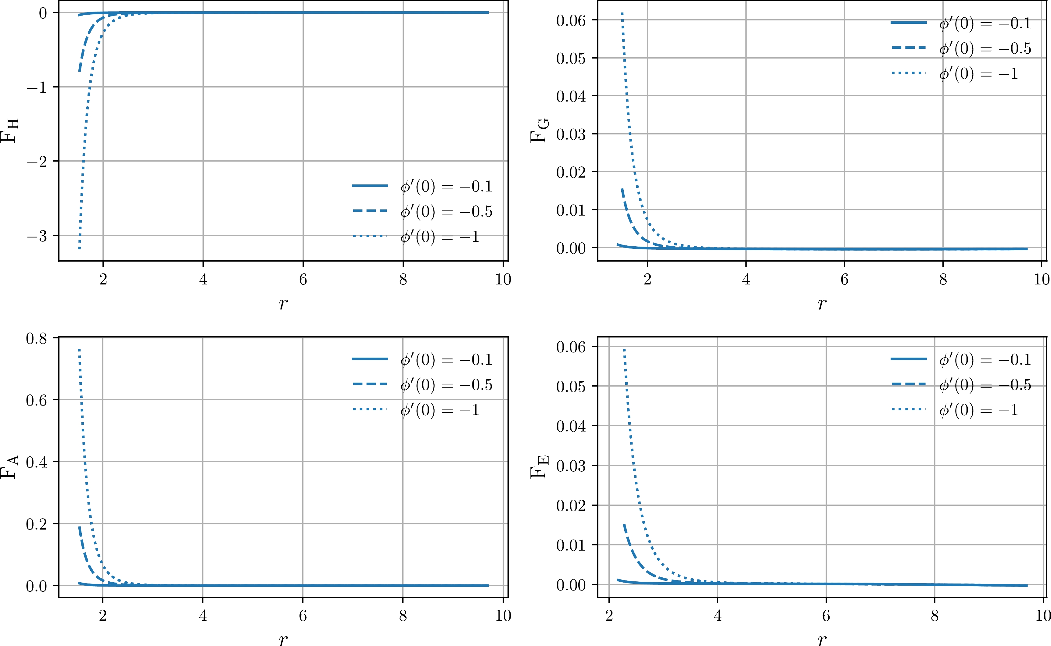
Figure 11. (color online) Forces present in the modified TOV equilibrium for Finch-Skea star coupled to the KB field.
-
Finally, in this subsection, we probe the behavior of the adiabatic index for our stellar solutions. Numerical results are plotted in Fig. 12. Note that our stellar solution is stable everywhere except for the regions where the adiabatic index numerical solution diverges.
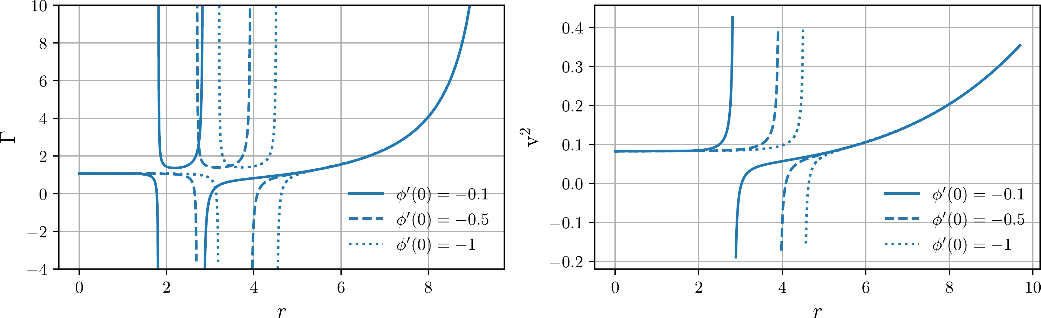
Figure 12. (color online) (first row) Adiabatic index for anisotropic Finch-Skea star coupled to KB field; (second row) sound of speed squared for anisotropic Finch-Skea star coupled to KB field.
-
As a final note on the minimal KB field in this subsection, we investigate the speed of sound for perfect fluid matter content inside a Finch-Skea compact star. Results of such investigation are plotted on the last, third plot of Fig. 12. According to the data from this plot, our fluid is relativistic. However, the speed of sound does not exceed the speed of light, which is required for the fluid to be viable. Note also that the values of
$ v^2 $ are generally smaller in the presence of the KB field (in relation to the classical GR). -
In this section, we present the final model of our consideration, namely gauged boson Finch-Skea star. This theory has a a gauge field
$ A_\mu $ admitting$ U(1) $ unitary symmetry and massless complex scalar field Φ with conical potential$ V(|\Phi|)=\lambda |\Phi| $ . For this type of model, the Lagrangian reads exactly as follows:$\begin{aligned}[b] {\cal{S}}[g,\Gamma,\Psi_i,\hat{\phi},A_\mu,\Phi]=&\int_{\cal{M}}{\rm d}^4x\sqrt{-g}\frac{1}{2\kappa^2}\big({\cal{R}}+{\cal{L}}(\Psi_i)\big)\\&-\frac{1}{4}\int_{\cal{M}}{\rm d}^4x\sqrt{-g}F^{\mu\nu}F_{\mu\nu} \\&-\int_{\cal{M}}{\rm d}^4x\sqrt{-g}({\cal{D}}_\mu \Phi)^*({\cal{D}}^\mu \Phi)-V(|\Phi|), \end{aligned} $

(54) where,
$ {\cal{D}}_\mu \Phi = \partial_\mu \Phi+{\rm i}eA_\mu \Phi, $

(55) $ F_{\mu\nu}=\partial_\mu A_\nu - \partial_\nu A_\mu . $

(56) An asterisk in an expression with gauge derivative denotes usual complex conjugation. For electromagnetic field
$ F_{\mu\nu} $ and massless scalar field Φ, equations of motion can be easily derived from the minimal action:$ {\cal{D}}_\mu(\sqrt{-g}F^{\mu\nu})=-{\rm i}e\sqrt{-g}[\Phi^*({\cal{D}}^\nu\Phi)-\Phi({\cal{D}}^\nu\Phi)^*], $

(57) $ {\cal{D}}_\mu(\sqrt{-g}{\cal{D}}^\mu\Phi)=\frac{\lambda}{2}\sqrt{-g}\frac{\Phi}{|\Phi|}, $

(58) $ [ {\cal{D}}_\mu(\sqrt{-g}{\cal{D}}^\mu\Phi)]^*=\frac{\lambda}{2}\sqrt{-g}\frac{\Phi^*}{|\Phi|}. $

(59) Finally, it is also useful to define the stress-energy-momentum tensor for gauge and complex scalar fields respectively [ 51]:
$ T_{\mu\nu}^F=E_{\mu\nu}=-g_{\mu\nu}{\cal{L}}_F+\frac{2\partial {\cal{L}}_F}{\partial g^{\mu\nu}}=F_{\mu\alpha}F_\nu^{\;\alpha}-\frac{1}{4}g_{\mu\nu}F_{\alpha\beta}F^ {\alpha\beta}, $

(60) $\begin{aligned} T_{\mu\nu}^\Phi=&({\cal{D}}_\mu\Phi)^*({\cal{D}}_\nu\Phi)+({\cal{D}}_\mu\Phi)({\cal{D}}_\nu\Phi)^*\\&-g_{\mu\nu}[({\cal{D}}_\alpha\Phi)^*({\cal{D}}_\beta\Phi)g^{\alpha\beta}-g_{\mu\nu}\lambda |\Phi|]. \end{aligned} $

(61) Throughout the paper, we have assumed vanishing electromagnetic strength tensor
$ F_{\mu\nu}=0 $ . For that purpose, we can use the following anzatz:$ \Phi(t,r)=\phi(r){\rm e}^{{\rm i}\omega t},\quad A_{\mu}(x^\mu){\rm d}x^\mu = A(r){\rm d}t . $

(62) Therefore, field equations for gauged boson Finch-Skea fluid sphere are expressed in the following form [52]:
$ \kappa\rho= \left[{\rm e}^{-\nu} \left(\omega+qA\right)^2\right] \phi^2+\frac{ {\rm e}^{-\lambda-\nu} (A')^2}{2}+ \phi'^2 {\rm e}^{-\lambda}, $

(63) $ \kappa p_r = \left[-{\rm e}^{-\nu} \left(\omega+qA\right)^2\right] \phi^2+\frac{{\rm e}^{-\lambda-\nu} (A')^2}{2}- \phi'^2 {\rm e}^{-\lambda}, $

(64) $ \kappa p_t =\left[-{\rm e}^{-\nu} \left(\omega+qA\right)^2\right] \phi^2-\frac{{\rm e}^{-\lambda-\nu} (A')^2}{2}+ \phi'^2 {\rm e}^{-\lambda}. $

(65) We can also properly derive field equations for gauge (Maxwell) and scalar (Klein-Gordon) fields:
$ A''+\left( \frac{2}{r}-\frac{\nu'+\lambda'}{2}\right)A'-2 q {\rm e}^{\lambda} \phi^2 \left(\omega+qA\right)=0, $

(66) $ \phi''+\left( \frac{2}{r}+\frac{\nu'-\lambda'}{2}\right)\phi'+ {\rm e}^{\lambda} \left[ \left(\omega+qA\right)^{2}{\rm e}^{-\nu}\right]\phi=0. $

(67) As initial conditions, we have chosen the case with
$\phi(0)=A(0)=\rm const$ and$ \phi'(0)=A'(0)=0 $ . In the next subsection, we match the interior stellar and exterior Reissner-Nördrstrom spacetimes. -
Given that we added minimally coupled
$ U(1) $ gauge field to our total Lagrangian, we need to redefine the junction conditions in the presence of interior charge. This time, we will match interior and exterior spacetimes using the Reissner-Nördstrom metric tensor (which describes charged spherically symmetric vacuum), for which the line element reads$\begin{aligned}[b] {\rm d}s^2 =& \bigg(1-\frac{2M}{R}+\frac{Q^2}{R^2}\bigg){\rm d}t^2 - \bigg(1-\frac{2M}{R}+\frac{Q^2}{R^2}\bigg)^{-1}{\rm d}r^2 \\&- r^2 {\rm d}\theta^2 - r^2 \sin^2 \theta {\rm d}\phi^2 .\end{aligned} $

(68) Here, Q is the total charge of the system, which is defined as
$ Q=\int^R_0j^t\sqrt{-g}{\rm d} r, $

(69) where
$ j^t $ is the only non-vanishing component of four-current (Noether current) in the static spacetime. This current can be expressed as follows:$ j^\mu = -{\rm i}e[\Phi({\cal{D}}^\mu\Phi)^*-\Phi^*({\cal{D}}^\mu\Phi)]. $

(70) With the use of a spherically symmetric line element of the stellar spacetime, we can rewrite the expression for total charge:
$ Q=8 \pi q\int^{R}_{0}{\rm d}r r^2 \left(\omega+qA\right)\phi^2 {\rm e}^{\frac{\lambda-\nu}{2}}. $

(71) To numerically solve the field equations and coupled differential equations for scalar and gauge fields, we need to assume a value for charge Q. Given that we are working in the RS spacetime,
$ Q<M $ . Using the RS line element, we can impose continuity conditions at the boundary:$ {\rm{Continuity\;of}}\;g_{tt}:\quad 1-\frac{2M}{R}+\frac{Q^2}{R^2}={\rm e}^{\nu(r)}, $

(72) $ {\rm{Continuity\;of}}\;\frac{\partial g_{tt}}{\partial r}:\quad \frac{2M}{R^2}-\frac{2Q^2}{R^3}=-B \left(2 A \sqrt{C R^2}+B C R^3\right), $

(73) $ {\rm{Continuity\;of}}\;g_{rr}:\quad \bigg(1-\frac{2M}{R}+\frac{Q^2}{R^2}\bigg)^{-1}={\rm e}^{\lambda(r)}, $

(74) $ {\rm{Vacuum\;condition}}:\quad p\rvert_{r=R}=0 .$

(75) Solutions for the above conditions are as follows:
$ \begin{gathered} A=\frac{\sqrt{R (R-2 M)+Q^2}}{R}-\frac{1}{2} B R \sqrt{C R^2} , \end{gathered} $

(76) $ \begin{gathered} B=\frac{C \left(M R-Q^2\right)}{\left(C R^2\right)^{3/2} \sqrt{R (R-2 M)+Q^2}} , \end{gathered} $

(77) $ \begin{gathered} C=\frac{1}{-2 M R+Q^2+R^2}-\frac{1}{R^2} . \end{gathered} $

(78) We use these junction conditions to numerically investigate our model in the next subsections.
-
Null, Dominant, and Strong energy conditions are plotted in Fig. 13. It is evident that, in our case, only one energy condition, namely the null energy condition for radial pressure, is satisfied. Some of other violated ECs could be satisfied for larger values of ω and different initial conditions for
$ A(r) $ and$ \phi(r) $ , but in that case,$ v^2>c^2 $ , which is unacceptable. Note also that, if we vary the values of the Noether charge obeying the inequality$ |Q|<M $ , the results will not change significantly, and ECs will be still validated/violated.
Figure 13. (color online) Null, Dominant, and Strong energy conditions for Finch-Skea PSRJ1416-2230 star minimally coupled to
$ U(1) $ gauge field and massless complex scalar field. To numerically derive$ T_{\mu\nu} $ components, we assumed$ Q=0.5 $ and$ \omega=10^{-6} $ . -
In this subsection, we study the radial derivatives of energy density, pressures, and equation of state for Finch-Skea star minimally coupled to
$ U(1) $ gauge field, massless complex scalar field. The results are shown in Fig. 14. From these plots, we can conclude that the radial fluid behaves like dark energy and tangential like stiff fluid. Gradients are positive for radial pressure and negative for energy density and tangential pressure.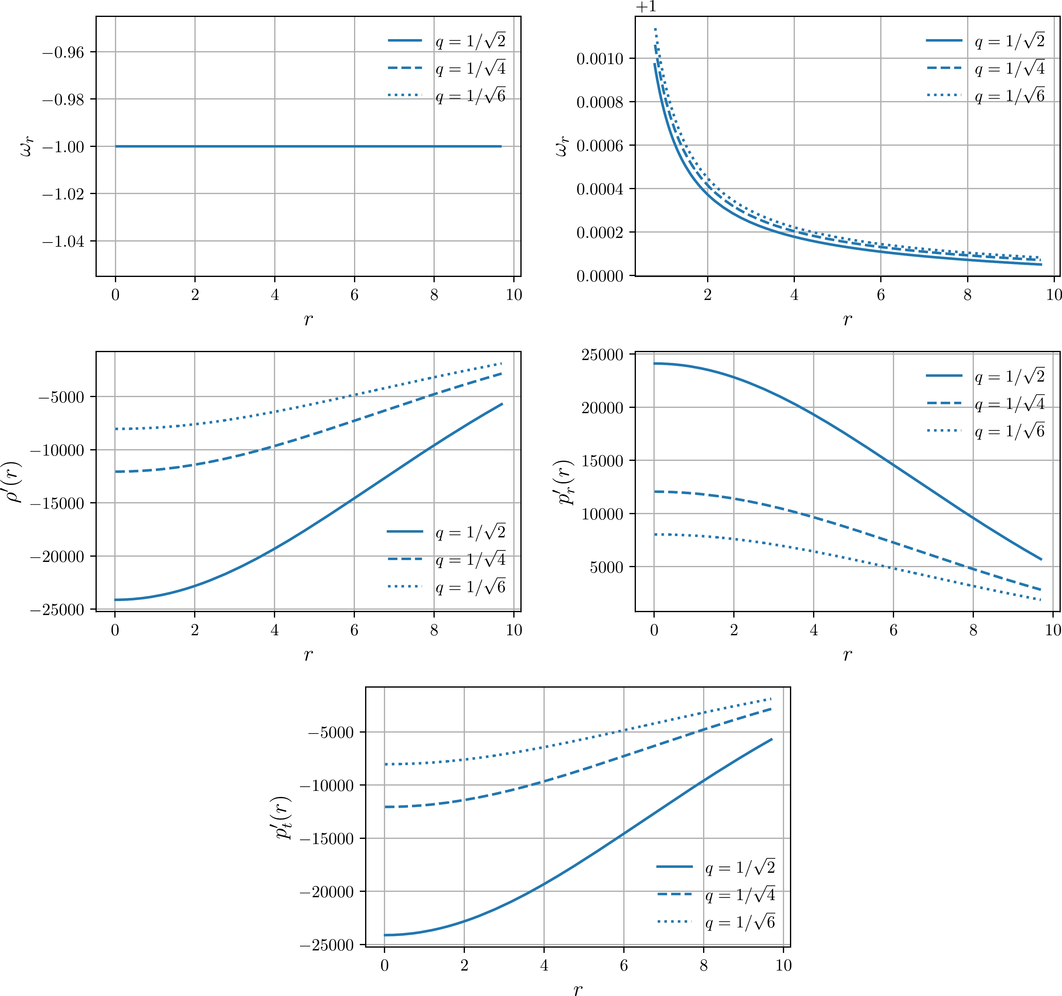
Figure 14. (color online) Equation of state and radial derivative of stress-energy tensor components for Finch-Skea star coupled to
$ U(1) $ gauge field and massless complex scalar field. To numerically derive the solutions, we assumed$ Q=0.5 $ and$ \omega=10^{-6} $ . -
We probed the stability of our stellar matter content through the well known modified TOV equation. We depict the results of TOV forces in Fig. 15. For the particular case of presence of gauge field, all the forces except for the extra one are negative.

Figure 15. (color online) Forces present in the modified TOV equation for Finch-Skea star coupled to
$ U(1) $ gauge field and massless complex scalar field. To numerically derive the solutions, we assumed$ Q=0.5 $ and$ \omega=10^{-6} $ . -
In this subsection, we study the stability of our stellar matter content from continuous adiabatic perturbations. The numerical solution for the adiabatic index is shown in the first plot of Fig. 15. Note that the adiabatic index satisfies the
$ \Gamma>4/3 $ constraint, so our stellar solutions in the presence of gauge field can be considered as stable from adiabatic perturbations. -
Finally, we probed the speed of sound, as shown in the last plot of Fig. 16. Note that, in our case, the fluid is ultrarelativistic but does not exceed unity, which is a required condition.

Figure 16. (color online) Anisotropic adiabatic index and speed of sound for Finch-Skea star coupled to
$ U(1) $ gauge field and massless complex scalar field. To numerically derive the solutions, we assumed$ Q=0.5 $ and$ \omega=10^{-6} $ . -
Given that the junction conditions change, the surface redshift will also vary. The surface redshift is depicted in Fig. 17 for different values of total charge Q. During the numerical analysis, the surface redshift for charged stars was smaller than that for uncharged ones; consequently, as
$ |Q|\to\infty $ ,$ {\cal{Z}}_s\to 0 $ .
Figure 17. (color online) Surface (gravitational) redshift for gauged Finch-Skea stellar interior (the parameter values are the same as those for ECs). The solid line represents the solution for
$ Q=0.9 $ , and the dashed line represents the solution for$ Q=1 $ . -
In this study, we investigated the spherically symmetric and static stellar solutions imposing Finch-Skea symmetry in the presence of exotic matter fields such as Bose-Einstein Condensate, Kalb-Ramond antisymmetric tensor field, and gauge field with local
$ U(1) $ gauge symmetry. To numerically solve numerous equations and graphically plot the results, we used compact star PSRJ1416-2230, which has a mass$ M=1.69M_\odot $ and radius$ R=9.69R_\odot $ . Next, we summarize the main results of our study:● Energy Conditions: for Bose-Einstein Condensate, Null and Strong energy conditions for both radial and tangential pressures were satisfied, so there is no exotic fluid in the stellar interior. For the sake of causality, the energy conditions considered in this study were violated for the Kalb-Ramond field and only radial NEC was validated for the gauge field. We represent the energy conditions for each exotic matter field of our consideration in Figs. 4, 9 and 13.
● Equation of State: for BE Condensate, the radial EoS parameter is regular; in asymptotical terms,
$ \phi'(0)\to-\infty $ , which describes a Zeldovich fluid; in tangential asymptotical terms, it describes a ΛCDM dark energy like fluid. For a Kalb-Ramond fluid, the situation is different. The radial EoS is regular and vanishes at the envelope; the tangential one is negative at the stellar core and regular at the intermediate envelope regions. Finally, for the gauge field, the radial EoS describes a DE-like fluid for any$ |q|\in\mathbb{R} $ , and the tangential one describes a fluid with an EoS that slightly deviates from the Zeldovich one; as$ q\to0 $ ,$ \omega\to1 $ . For further information and graphical representations of these results, refer to Figs. 5, 10, and 14(first row).● Gradients of perfect fluid stress-energy tensor components: radial gradients are negative for energy density and radial pressure, and positive for the tangential one in presence of BEC. For the KB field, the situation is opposite, namely
$ \rho'(r)\land p_r'(r)\geq0 $ and$ p_t(r)\leq0 $ . Finally, for the$ U(1) $ gauge electromagnetic field, the energy density and tangential gradients were negative, and the radial was positive. Numerical evidence for these statements can be found in Figs. 5, 10, and 14.● TOV equilibrium: we also probed the dynamical stability of our stellar object with minimally coupled exotic fields. For BEC, we observed that only hydrodynamical and extra forces were positive, and the rest of the forces were negative. Moreover, the vast contribution to the total TOV provided fluid anisotropy. By contrast, for the KB field, there was only one negative force, namely the hydrodynamical force, which was also the strongest one. Finally, for the gauge field, only the extra force was positive. The results are properly depicted in Figs. 6, 11, and 15.
● Adiabatic index: we also studied the stability of anisotropic matter inside compact stars in the presence of adiabatic perturbations. It was shown that
$ \Gamma>4/3 $ for relatively large and negative initial conditions for the scalar field$ \phi'(0) $ in the case of BEC. Moreover, for the KB star, this parameter is stable everywhere except for the diverging regions. Finally, for gauge field stars, it is stable everywhere. Plots of Γ over the whole interior radial domain are shown in Figs. 7, 12, and 16.● Sound of speed: the last quantity that we discussed was the speed of sound. For objects to obey the causality condition,
$ v^2\leq c^2 =1 $ . For BEC, KB, and gauge fields, this necessary condition was validated everywhere, as expected. The squared speed of sound is depicted in the second plot of Figs. 7, 12, and 16.At this point, it is useful to compare our results with existing ones obtained for other compact star geometries. Numerous studies on compact stars have been conducted within the General Theory of Relativity. However, we focus on the solutions that are close to ours. For example, one could introduce Einstein-Klein-Gordon stars (compact stellar solutions endangered by a scalar field), Einstein-Maxwell stars (analogically, stars endangered by a Maxwell field that usually respects some gauge symmetries), or Boson/Proca stars as the closest "siblings" to our solutions.
For Einstein-Maxwell Buchdahl stars, a good study on the GR theory is presented in Ref. [53]. In comparison with our results for stars with
$ U(1) $ background field, their solution respected all energy conditions. Moreover, because of the isotropy of their stellar solution, anisotropic forces in TOV vanished, and the hydrodynamical force was positive. Speed of sound squared had similar behavior to ours, but the rate of change with r was significantly larger. The EoS parameter was positive for$ \omega\in(0,1) $ . Finally, the adiabatic index also had many larger values, but the inequality$ \Gamma>4/3 $ holds for both ours and their solutions.By contrast, bosonic stellar solutions were not comprehensively analyzed in the existing literature within the General Theory of Relativity. However, some studies were developed within the Einstein-Scalar-Gauss-Bonnet (ESGB) theory, which is a viable theory of gravitation. For example, in Ref. [54], isotropic ESGB stellar solutions were probed. By comparing the aforementioned model with our BEC stellar configuration, we conclude that ECs for both models presented the same behavior in practical terms and asymptotically vanished. However, in the EGSB case,
$ v^2 $ and Γ are monotonically decreasing functions, while, in our case, they grow near the stellar envelope. Moreover, for the case with Gauss-Bonnet corrections, the surface redshift was negative, while, in our case, it was positive and decreased up to the envelope.To date, there are no comprehensive studies (including investigations on ECs, EoSs, and adiabatic and TOV stabilities) within the GR for stellar configurations such as Boson/Proca stars. However, from Ref. [55], we conclude that, similar to our case, both Boson and Proca stars have positive energy density with the peak at the stellar origin, and that
$ \rho\to0 $ asymptotically with the radial coordinate; this was observed in our case as well. Moreover, magnetized BEC stars were investigated in Ref. [56]. In comparison to our BEC star solution, the magnetized one has a smaller surface redshift and both positive pressure and density with$ \rho\gg p $ . Thus, NEC/WEC/SEC and DEC are satisfied.From the aforementioned results and graphical representations, it is clear that our stellar solution is of non-singular nature and exhibits interesting properties in physically interesting and viable models, such as GR expanded using exotic matter fields (BEC dark matter, KB field from string theory, and gauge fields from electromagnetism). However, in future studies, it will be interesting to probe such models with Dirac spinor fields and QCD Axions, as well as in the presence of non-homogeneous oscillating axion fields with large scale correlations.
-
We are very grateful to the honorable referee and editor for their meaningful suggestions that have significantly improved our work in terms of research quality and presentation.
Compact stars admitting Finch-Skea symmetry in the presence of various matter fields
- Received Date: 2022-08-05
- Available Online: 2023-01-15
Abstract: In the present study, we investigate the anisotropic stellar solutions admitting Finch-Skea symmetry (viable and non-singular metric potentials) in the presence of some exotic matter fields, such as Bose-Einstein Condensate (BEC) dark matter, the Kalb-Ramond fully anisotropic rank-2 tensor field from the low-energy string theory effective action, and the gauge field imposing


 DownLoad: