


 Abstract
 HTML
HTML Reference
 Related
 PDF
PDF


-
The formation of a primordial black hole (PBH) in an inflationary period consisting of a preheating period offers an intriguing window for exploring the early universe [1–3]. From another perspective, the PBH could account for the formation of dark matter (DM) according to the abundance of PBHs [4–9]. The explicit observation of gravitational waves is the most essential achievement by the joint LIGO/Virgo collaboration, especially for merged black holes (BHs) [10–12] whose mass ranges are approximately
$ 30 M_{\odot} $ , which cannot be explained by stellar evolution. However, the mass range of PBHs could cover this mass; thus, the PBH is of significance to exploring the formation of BHs [5, 13, 14]. The mass range from$ 10^{-17}-10^{-15} M_{\odot} $ and$ 10^{-15}-10^{-13} M_{\odot} $ can almost explain the origin of DM because these scales cannot be constrained by observations. PBHs are usually formed by the gravitational collapse of an overdense region. This leads to a large amplitude of curvature perturbation at certain scales, which can be realized by tuning the background dynamics of the quantum field in the inflationary universe [15–25]. Owing to their specification, PBHs may leave imprints for the observation,$ \it e.g. $ , the seeds for the formation of a galaxy, and the evaporation of PBHs may interestingly interpret the observations of point-like gamma-ray sources [26, 27].There are several methods of realizing the mechanism behind enhancing the power spectrum at small scales. One effective method, known as ultra-slow-roll inflation [28, 29], especially for the inflection point of the potential [30], has been dubbed as a highly economical way of generating an enhanced power spectrum [31–33]. Under this framework, it is not explicitly realized a viable mechanism for keeping the e-folding number is at approximately
$ 50-60 $ [34, 35]. Another way of enhancing the power spectrum is by implementing the non-minimal coupling and noncanonical kinetic term [36–42], in which the potential and non-minimally coupling function should have a special form with fine-tuned parameters for various models. In light of k [43, 44] and G inflation [45, 46], there is a new mechanism for generating a large power spectrum under the framework of noncanonical kinetic terms at small scales, known as resonant sound speed during inflation. This is different from the standard procedure for the preheating period, in which the resonant sound speed appears during the early inflationary period ($ \Delta N $ is approximately$ 10 $ ) [47]. Owing to its simplicity and richness from phenomenology, it can be applied to stochastic gravitational waves [48], and this mechanism can be embedded into DBI inflation [49] and curvaton-inflaton mixed inflation [50]. A similar mechanism was proposed for a case in which the sound speed approaches zero at some stage of inflation in single field inflation [33, 51]. The amplification of curvature perturbation could also arise from the oscillation potential [52]. Even the PBH can be formed due to peak theory [53].To investigate the formation of PBHs, we require the amplification of curvature perturbation resulting from inflationary perturbation, in which broad types of single-field inflationary theories are highly relevant to the shape of inflation. To relax this stringent condition, a curvaton model was proposed in which curvature perturbation arises from the curvaton [54–56] and is usually considered an independent field. Consequently, it may account for various particles,
$ \it i.e. $ , the axion field [57], could form an axionic PBH owing to the role of the axion [50, 58, 59]. Considering the preheating process, we assume that the curvaton field originates from inflaton decay [60–66]. If considering the multifield framework for the curvaton [67], we can also investigate the impact of the noncanonical kinetic term. Moreover, this paper also aims to unify DM and dark energy (DE) in light of our previous study. From a thorough investigation of the curvaton field, from its generation up to the DE epoch, we provide a full analysis of curvaton evolution.This paper is organized as follows: In Sec. II, we revise the running curvaton mechanism. In Sec. III, we investigate the formation of PBHs in light of the Mathieu equation. In Sec. IV, we give a simple analysis of the late time evolution of the curvaton. Finally, Sec. V contains the conclusion and discussions.
We work in natural units, in which
$ c=1=\hbar $ , but retain the Newton constant G. -
We investigate the formation of PBHs during the preheating period. The main feature used to realize this process is the coupling between the curvaton field and the potential of inflation. Subsequently, we can utilize the Mathieu equation to explore the formation of PBHs during the preheating period. Recently, a similar mechanism for realizing the formation of PBHs was used based on the stability of the Mathieu equation [68].
-
Before discussing the formation of PBHs, we first revisit the running curvaton model. At the very beginning, there is only one field, known as the inflaton. Then, the curvaton field appears via the decay of the inflaton. Meanwhile, the explicit coupling between the inflationary potential and curvaton field is different from traditional coupling (Yukawa coupling for scalar fields). Moreover, we add an exponential potential for the curvaton field to depict the dynamical behavior of DE. Therefore, the total action can be written as
$ \begin{aligned}[b] S=&\int {\rm d}^{4}x\sqrt{-g}\Bigg\{\frac{M_{P}^{2}}{2}R-\frac{1}{2}g^{\mu\nu}\nabla_{\rm{{\mu}}}\phi\nabla_{\nu}\phi-\frac{1}{2}g^{\mu\nu}\nabla_{\rm{{\mu}}}\chi\nabla_{\nu}\chi\\& -V(\phi)-\frac{g_0}{M_{P}^{2}}\chi^{2}V(\phi)-\lambda_{0}\exp\Bigg[-\lambda_{1}\frac{\chi}{M_{P}}\Bigg]\Bigg\}, \end{aligned} $

(1) where χ and ϕ are the curvaton and inflaton, respectively, R represents the Ricci scalar, g is the determinant of
$ g_{\mu\nu} $ , and$ g_0 $ ,$ \lambda_0 $ , and$ \lambda_1 $ are the dimensionless parameters determined by observations in the Lagrangian. It should be emphasized that$ \lambda_0 $ is implemented to mimic the dynamical behavior of DE; thus, it is of the order of$ 10^{-120} $ in Planck units. Our curvaton model is realized in the preheating period for which the inflaton oscillates its potential. The energy can then be transformed into the curvaton field. As shown in [69], because the inflaton oscillates near its minimal point, the various inflationary potentials can be approximated as$ V(\phi)\approx \frac{1}{2}m^2\phi^2, $

(2) where m is the effective mass of the inflaton, determined using
$\dfrac{{\rm d}^2V(\phi)}{{\rm d}\phi^2}$ . Thus, our curvaton mechanism can be embedded into many inflationary models, in which action (1) clearly shows that the explicit coupling term$ \dfrac{g_0\chi^2}{M_{P}^2}V(\phi) $ consists of many forms. Owing to this explicit coupling, the effective mass of the curvaton can be easily obtained using$ m_{\rm \chi}^ 2\approx\frac{g_0}{M_{P}^2}V(\phi), $

(3) where we neglect the contribution of the exponential part of the curvaton potential because it is too small before the inflaton finishes the decay. This mass parameter will play a significant role in simulating the formation of PBHs in the preheating period.
As we know, the wavelength expands slowly compared to the Hubble radius; thus, the perturbation mode of the curvaton will cease at the subhorizon. To re-enter the horizon, the second inflationary process is necessary to achieve the re-entering into the horizon. In the next subsection, we illustrate this process via the interaction between the curvaton and other particles.
-
The second inflation is highly relevant to the evolution of the background (for the inflaton and curvaton). To obtain a viable process of enhancing the power spectrum, we first require an interaction that is similar to action (1),
$ \mathcal{L}_{\rm int}=\frac{1}{2}m_{\chi}^2\chi^2+\frac{g_1}{M_{\rm Pl}}\varphi^2V(\chi), $

(4) where φ is a type of scalar particle (
$ \it e.g. $ , an ultra light scalar particle), and$ g_1 $ is the dimensionless parameter.Following Ref. [70], we divide the preheating period into two parts: (a) The first preheating arises via the oscillation of the inflaton after inflation, which is known as the ϕD or RD1 era. (b) The second inflation is driven by the curvaton potential energy after χD, dubbed as the χD or RD2 era. For the occurrence of the second condition, the initial amplitude of the curvaton must be sufficiently large. We must also figure out which background will be alternated by the second inflation process. As noted in [70], the curvaton model can be classified into three types: the large field type (
$ m_\chi> M_{\rm Pl} $ ), small field type ($ m_\chi< M_{\rm Pl} $ ), and hybrid field type (the coupling between the curvaton and inflaton). They obtained the most general cases of the curvaton scenario. In this paper, we focus on the hybrid field type. According to their explicit calculation, we can find that$ N_e $ (e-folding number) will be enlarged to approximately$ 70 $ , which is important for our analysis of the formation scale of PBHs during the second inflation process. As for its observables, the spectral index$ n_\chi $ decreases in the hybrid type of the curvaton model. Here, we focus on its curvature perturbation in the second inflation.After introducing the second inflation, the curvature perturbation induced by the curvaton re-enters the Hubble radius. Consequently, the enhanced density perturbation may have a longer collapsing time into the PBH after re-entering the horizon.
-
In this subsection, we obtain the equation of motion (EOM) of the
$ \delta\varphi $ field (quantum fluctuation of some spectator field) from action (1). Here, we define$ \varphi(x,t)=\bar{\varphi}(t)+\delta\varphi(x,t) $ , where$ \bar{\varphi}(t) $ denotes the background of a spectator scalar particle depending only on time, and$ \delta\varphi(x,t) $ is the quantum fluctuations. After this definition, varying it with action (1), and transferring into momentum space, we get$ \left(\delta\ddot{\varphi}_{k}+3\frac{\dot{a}}{a}\delta\dot{\varphi}_{k}\right)+\frac{k^{2}}{a^{2}}\delta\varphi_{k}+m^{2}_\chi\frac{g_1}{M_{P}^{2}}\chi^{2}\delta\varphi_{k}=0, $

(5) where there is an extra term,
$ \dfrac{k^2}{a^2}\delta\varphi_k^2 $ , compared with the EOM of$ \bar{\varphi}(t) $ , in which we will analyze the quantum fluctuations of the spectator field. Subsequently, we can utilize the EOM of the background of the curvaton field$ \chi\approx \chi_0a^{-2/3}\sin(mt) $ in the preheating period and rearrange Eq. (5). Then, we can obtain the following equation:$ \delta\ddot{\tilde{\varphi}}_{k}+\left(\frac{k^{2}}{a^{2}}\right)\delta\tilde{\varphi}_{k}+\frac{g_0m^{2}_\chi}{2M_{P}^{2}}\chi_{0}^{2}\delta\tilde{\varphi}_k-\frac{m^{2}_\chi g_1}{2M_{P}^{2}}\delta\tilde{\varphi}_k\chi_{0}^{2}\cos(2m_{\chi}t)=0. $

(6) Finally, by setting
$ z=m_{\rm \chi}t $ and$ \delta\tilde{\varphi}_k=a^{3/2}\delta\varphi_k $ , Eq. (6) becomes$ \delta\tilde{\varphi}_{k}''+(A_{k}-2q_{k}\cos[2z])\delta\tilde{\varphi}_{k}=0 $

(7) where the correspondence can be found as
$ A_{k}=\frac{k^{2}}{m_{\chi}^{2}a^{2}}+\frac{g_1\chi_{0}^{2}}{2M_{P}^{2}}, $

(8) $ q_{k}=\frac{\chi_{0}^{2}g_1}{4M_{P}^{2}}. $

(9) Thus, Eq. (9) can become the standard form of the Mathieu equation. There is a key feature of the Mathieu equation in which the solution of Eq. (7) is proportional to
$ \varphi_k\propto \exp[\mu_k^{(n)} z]=\exp[\mu_k^{(n)}m_{\rm \chi }t], $

(10) where
$ \mu_k^{(n)} $ is the Lyapunov index depicting the n th instability band of the Mathieu equation, in which the first band is sufficient for investigating the production of the PBH, and its corresponding formula at the first band is denoted by$ \mu_k=\sqrt{\dfrac{q_k^2}{4}-\left(\dfrac{2k}{m_\chi}-1\right)^2} $ , following the notation of Ref. [65]. Resonance occurs at$ k=\dfrac{m_\chi}{2} $ , and the first band may take the maximal value of$ \mu_k=\dfrac{q_k}{2} $ considered in the following calculation (namely,$ m_\chi=2k $ ), where m is the mass of the inflaton in this paper. The solution$ \chi_k $ becomes$ \varphi_k\propto \exp \left[\frac{q_k m_\chi t}{2}\right]=\exp[q_k kt], $

(11) which is analyzed for PBH formation. Moreover, we observe that the formation of PBHs is highly relevant to the curvaton mass
$ m_\chi $ . Here, we connect k to the curvaton mass m. Owing to the instability (11), this is key for ensuring the formation of PBHs at certain scales, which is considered an enhanced part of the power spectrum of the curvaton and will not impact CMB observation [71].In this section, we revisit a large class of curvaton scenarios, known as the running curvaton, in which there is a second inflationary process to forming the PBH because the initial amplitude of the curvaton is sufficiently large. During the second inflation, the mass of the curvaton plays a significant role for the scale of PBH formation.
-
In this section, we investigate the formation of PBHs considering the instability of the Mathieu equation. Before performing a detailed calculation, we first give a simple physical picture of the formation of PBHs. Recall that the formation occurs during the preheating period, and the energy of the curvaton is transferred into other spectator fields that derive the second inflation. The mass of the curvaton plays a role in the instability band.
The super Hubble scale or sub Hubble scale is determined by the comoving Hubble radius
$ \mathcal{H}=a H $ , with$\mathcal{H}=\dfrac{{\rm d}a}{{\rm d}\tau}$ (τ is the conformal time) and$H=\dfrac{{\rm d}a}{{\rm d}t}$ (t is the physical time). Combined with our analysis for the formation of the PBH during the second inflation, the modes of the quantum fluctuations of the curvaton field re-enter the horizon ($ \mathcal{H}^{-1} $ as the horizon). In our calculation, we utilize the physical time t. Thus, the evolution of the power spectrum varies with respect to$ \tilde{k}=\dfrac{k}{a} $ not k. A previous analysis has shown that the background of inflation alternates; in particular, the e-folding number changes to approximately$ 70 $ . Therefore, we use this number as a reasonable input to analyze our Hubble radius. -
One of the most essential processes in producing the PBH is enhancing the value of the power spectrum at certain scales beyond CMB constraints. In this paper, we utilize the instability of the Mathieu equation to obtain a satisfying power spectrum.
To obtain the full power spectrum considering this instability, we recall the content of the power spectrum using the
$ \delta N $ formalism, the corresponding formula of which is$ P_\zeta=\dfrac{H_*^2}{9\pi^2}\dfrac{r_{\rm decay}^2}{\chi^2} $ (where$ H_*^2 $ denotes the value at the freezing time of the Hubble radius, and χ denotes the value of the curvaton when it begins to oscillate). Here, the range of$ P_\zeta $ is consistent with observations when taking$ 0.12<r_{\rm decay}<1 $ . In a single field inflationary model, the power spectrum can be obtained using$ P_\zeta=\dfrac{H^2_*}{8\pi^2\epsilon} $ , where$ \epsilon $ is of the order of unity after inflation. Comparing these formulas for the power spectrum, it is easily concluded that they are consistent with each other when taking$ 0.12<r_{\rm decay}<1 $ . Consequently, we can use$ P_\zeta=\dfrac{H^2_*}{8\pi^2\epsilon} $ as the first part of the full power spectrum, which can effectively recover the observations at large scales. Subsequently, we can follow standard procedure to rewrite$ P_\zeta=\dfrac{H^2_*}{8\pi^2\epsilon} $ in terms of$ A_s\bigg[\dfrac{\tilde{k}}{\tilde{k}_p}\bigg]^{n_s-1} $ , based on Ref. [72], where$ \tilde{k}_p $ is a fiducial comoving momentum with a value of approximately$ \tilde{k}_p=0.05\; {\rm{Mpc}}^{-1} $ .Here, we must emphasize that the power spectrum of our model is related to the energy scale k via
$ k=\dfrac{m_{\chi}}{2} $ , and the observable power spectrum is highly relevant to the comoving momentum. Consequently, we need$ k=a\tilde{k} $ to relate the power spectrum to the observations.From another perspective, we need the enhanced power spectrum at certain scales to simulate the generation of the PBH, similar to the mathematical property of Ref. [47] (the mechanism is different because their enhanced amplitude of curvature perturbation occurs at inflation). The power spectrum (mainly from the curvaton) experiences an exponential factor via instability (11) at certain scales
$ k_* $ ,$ P_\zeta=\dfrac{H^2_*}{8\pi^2\epsilon}\exp[q_kmt]= \dfrac{H^2_*}{8\pi^2\epsilon} $ $ \exp[2q_kk_{\rm scale}t]= \dfrac{H^2_*}{8\pi^2\epsilon}\exp[2q_k a \tilde{k}_{\rm scale}t] $ , where we adopt the definitions$ P_\zeta=k^3|\zeta_k|^2/(2\pi^2) $ and$ |\zeta_k|\propto v_k $ . Here,$ k_{\rm scale} $ ① represents certain scalesexplicitly related to the running mass m via (10). The mass only needs to be smaller compared with the upper limits of the inflationary potential from COBE normalization (an analysis is given later). Following Ref. [65], it is clearly indicated that$ \Delta k\propto q^l $ (where l is the l-th band of instability of the Mathieu equation), and in our case,$ q\ll 1 $ . Consequently, the enhanced part of the power spectrum can be parameterized by δ functions for some$ k_{\rm scale} $ . Taking these two factors into account, we can obtain the full formula of the power spectrum as$ \begin{aligned}[b] P_{\zeta}=&A_{s}\bigg[\frac{k}{k_{p}}\bigg]^{n_{s}-1}\bigg[1+\frac{q_k}{2}\exp\big(2q_kk_{\rm scale}t\big)\delta(k-2k_{\rm scale})\bigg] \\ =&A_{s}\bigg[\frac{k}{k_{p}}\bigg]^{n_{s}-1}\bigg[1+\frac{q_{\rm k}}{2}\exp(q_{\rm k}mt)\delta(k-m_\chi)\bigg]\\ =&A_{s}\bigg[\frac{k}{k_{p}}\bigg]^{n_{s}-1}\bigg[1+\frac{q_{\rm k}}{2}\exp(q_{\rm k}mt)\delta(a\tilde{k}-m_\chi)\bigg], \end{aligned} $

(12) where
$ A_s =\dfrac{H^2_*}{8\pi^2\epsilon} $ ,$ q_k $ is defined in Eq. (9) as the amplitude of the enhanced power spectrum, t is the physical time, and the coefficient of an exponential factor of$ \exp[q_kmt] $ arises from a triangle approximation. In the following calculation, we use the running mass as an input manifesting the main feature of our model. Once obtaining this full power spectrum, we can numerically simulate its range within the observational constraints.Figure 1 shows the varying trend of the full power spectrum (12), in which the black solid line corresponds to the observational value from COBE normalization [71] whose order is
$ 10^{-9} $ . In this figure, we give three values of$ \tilde{k} $ as an illustration of PBH formation. To relate the realistic energy scale, we unify$ \rm Kpc^{-1} $ into$ \rm GeV $ . We take$ \tilde{k}_3 $ as an example, for which it is straightforward for obtain$\tilde{k}_3\approx 10^{-26}\; \rm GeV$ . Keeping in mind that our Universe has experienced exponential inflation and is continuously expanding, the scale factor is a monotonically increasing function. Compared with the reheating and preheating periods, the expansion of inflation is considerably larger. Thus, we use$ a(t_*)=\exp(70) $ (the inflation will last nearly$ N=70 $ ) as an approximation to obtain the energy scale$ k_*=a(t_*)\tilde{k}_3\approx 10^{13}\; \rm GeV $ , whose value is consistent with the energy scale of the reheating or preheating period (depending on various models). The realistic value of$ k_* $ will be larger than this value because we set this approximation.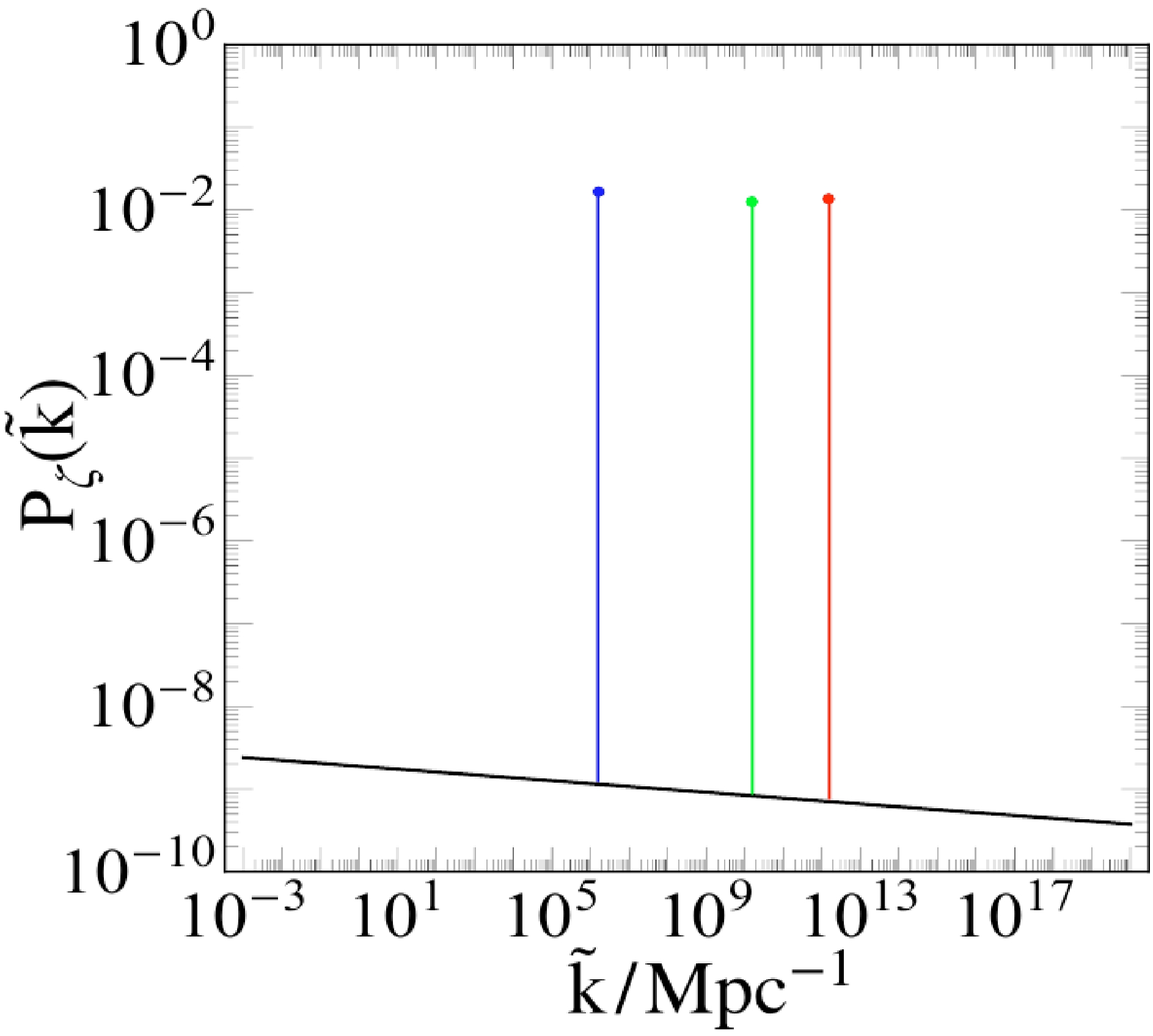
Figure 1. (color online) Plot of power spectrum (12): The horizontal line corresponds to the energy scale with a range of
$ 10^{-7} \rm\; Mpc^{-1}\leqslant k\leqslant 10^{20}\; {\rm{Mpc}}^{-1} $ . The vertical line denotes the value of$ P_\zeta $ , ranging from$ 10^{-10} $ to$ 1 $ . The black solid line represents the observational constraints taken from Ref. [71]. The blue, green, and red lines correspond to the enhanced part of the power spectrum by taking various masses of the inflaton.$ \tilde{k}_1=1.57\times 10^7\; {\rm{Mpc}}^{-1} $ is for the blue point, and$ \tilde{k}_2=1.6\times 10^{10}\; {\rm{Mpc}}^{-1} $ and$ \tilde{k}_3= 1.7\times $ $ 10^{12}\; {\rm{Mpc}}^{-1} $ correspond to the green and red points, respectively. The spectral index is set using$ n_s=0.965 $ .$ q_k\ll 1 $ .The various values of k may be determined by the original definition according to
$\mu_k= \sqrt{\dfrac{q_k^2}{4}-\left(\dfrac{2k}{m}-1\right)^2}$ , taking the maximal value of$ \mu_k $ . In particular, for the enhanced part of the power spectrum, its corresponding value can reach the order of$ 10^{-1} $ , which is sufficient for the generation of PBHs. All of these numerical simulations are performed with$ q_k\ll 1 $ , which belongs to narrow resonance. As for the choice of physical time, we set$ t=10^{2} $ s as a reasonable input because PBH formation occurs in the deep preheating period, which is after matter-radiation equality with$10\; {\rm s} < t<3\; {\rm {min}}$ .Additionally, this enhanced part of the power spectrum does not impact the observational constraints because the observational scale of the CMB is approximately located from
$ 10^{-5}\; {\rm{Mpc}}^{-1} $ to$ 10\; {\rm{Mpc}}^{-1} $ , which leads to consistency with observations. -
We utilize the enhancement of the primordial power spectrum to investigate the formation of PBHs in our theoretical framework. It can be clearly seen that we have large parameter spaces to construct the large amplitude of the power spectrum to collapse into the PBH, for which we give several specific values of curvaton mass and various
$ q_k $ , whose values are considerably smaller than one. This formation process occurs during the radiation period induced by the oscillation of the curvaton (the second inflation). Meanwhile, the PBH will be generated after the perturbations of curvaton re-entry into the horizon. The mass of the PBH, which is related to the horizon mass at horizon re-entry with various values of the co-moving wavenumbers k, is$ M(k)=\gamma \frac{4\pi}{\kappa^2 H}\approx M_{\odot}\bigg(\frac{\gamma}{0.2}\bigg)\bigg(\frac{g_*}{10.75}\bigg)^{-\frac{1}{6}}\bigg(\frac{k}{1.9\times 10^6\; {\rm{Mpc}}^{-1}}\bigg), $

(13) where
$ \kappa^{-1}=M_{\rm pl}=2.4\times 10^{18}\; \rm GeV $ is the reduced Planck mass, H is evaluated at$ k=a H $ (H is the Hubble parameter, and a is the scale factor), γ is defined as the ratio of PBH mass to horizon mass, indicating the efficiency of collapse, the value of which is approximately set as$ 0.2 $ from Ref. [73], and$ g_* $ is the degrees freedom of energy densities at PBH formation. Because its formation occurs during the preheating period, the process happens during the deep radiation period, whose value can be determined as$ g_*=106.75 $ . Here, we should emphasize the difference from the traditional curvaton mechanism, in which the curvaton is considered an independent field, leading to the decay of the curvaton after actual preheating. However, our model is different because the curvaton is generated and practically disappears as the inflaton decays; more precisely, the curvaton forms as the inflaton begins to decay, and the curvaton disappears as the inflaton finishes the decay process owing to the coupling between the curvaton and inflaton. During the entire process of inflaton preheating, the PBH is formed due to the instability of the curvaton. This is the reason we mention that this process occurs during the deep radiation period.To investigate the abundance of PBHs with mass M, we need the mass fraction
$ \beta(M) $ against the total energy at the formation of the PBH. Under the assumption of a Gaussian distribution, this can be expressed by [74, 75]$ \beta(M)=\frac{\rho_{\rm PBH}}{\rho_{\rm total}}=\frac{1}{2}\rm erfc\bigg(\frac{\delta_c}{\sqrt{2\sigma^2(M)}}\bigg), $

(14) where
$ \rm erfc $ is the complementary error function, and$ \delta_c $ denotes the threshold of perturbation at the formation of the PBH, the value of which is approximately$ 0.4 $ based on Refs. [76, 77]. References [78, 79] also proposed the value of$ \delta_c $ , and Refs. [80, 81] found that the value of$ \delta_c $ is also relavant with the compaction function, leading to a small deviation from$ 0.4 $ .$ \delta(M) $ is the variance of the density perturbation with mass M for the PBH, which can be associated with the power spectrum,$ \sigma^2(M(k))=\int {\rm d}\ln q W^2(qk^{-1})\frac{16}{81}(qk^{-1})^4 P_\zeta(q), $

(15) where
$ W(x)=\exp (-x^2/2) $ (Gaussian window function). Once we have these two physical quantities, we can define the abundance of PBHs, namely, the fraction of PBHs to total DM,$ f_{\rm PBH}=\frac{\Omega_{\rm PBH}}{\Omega_{\rm DM}}=2.0\times 10^8\bigg(\frac{\gamma}{0.2}\bigg)^{1/2}\bigg(\frac{10.75}{g_*}\bigg)^{1/4}\bigg(\frac{M_{\odot}}{M}\bigg)^{1/2}\beta(M), $

(16) where
$ \Omega_{\rm DM} $ is the current energy density of DM from the Planck 2018 results, with a value of approximately$ \Omega_{\rm DM}h^2 \approx 0.12 $ . In light of a basic estimation of the abundance of PBHs, the amount of the power spectrum of$ P_\zeta $ should reach the order of$ 10^{-2} $ to produce a sizable PBH abundance at small scales. For this, we provide our numerical simulation from Fig. 1.Figure 2 indicates the abundance of PBHs to the total energy density of DM in terms of the running curvaton scenario. There are three cases corresponding to the various masses, as shown in Fig. 1, the masses of which are
$ 10^{-12} M_\odot $ ,$ 10^{-8}M_\odot $ , and$ 10^{0} M_\odot $ . These the corresponding masses are obtained using the definition of$ \mu_k $ by taking its maximal value, namely,$ 2k=m $ , setting$ m_1 $ ,$ m_2 $ ,$ m_3 $ ,$ \rm e.t.c $ . Case one (red point) may result in the main component of DM, with a percentage of approximately$ 76.5\ $ % . In other words, it may account for DM to some extent. Cases 2 (green point) and 3 (blue point) are far from the observational constraints, especially compared with Kepler [88] and Subaru HSC [87]. Case 3 has a similar situation to the CMB [90]. However, Ref. [91] claimed that the mass range of the PBH is from$ 2 $ to$ 400 $ solar mass, which can only account for$ 0.2\ $ % DM. It was also discussed in [92] that the lower contribution of DM plays an important role and provides a significant probe for the early Universe.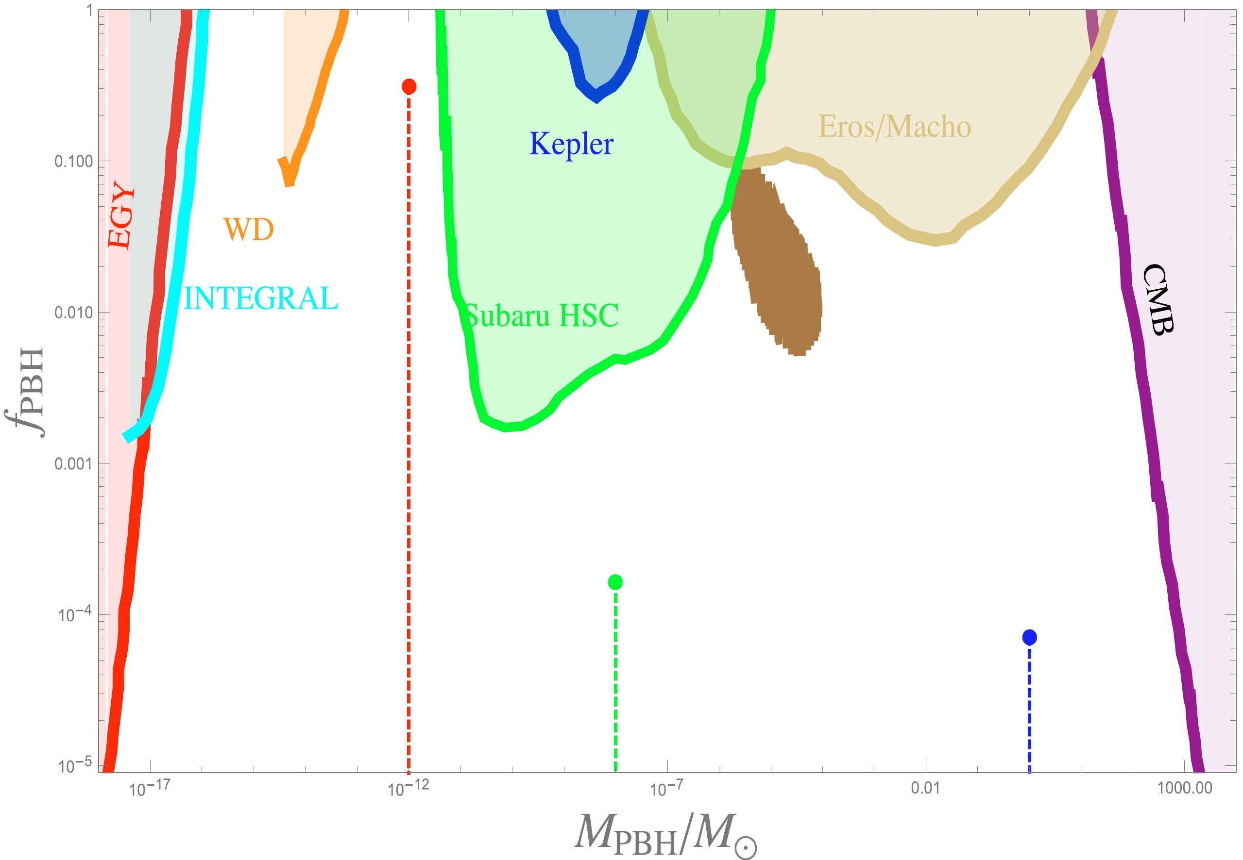
Figure 2. (color online) Plot of the abundance of PBHs (16): The horizontal line corresponds to the ratio of
$ M_{\rm PBH} $ to$ M_{\rm \odot} $ , whose range is from$ 10^{-19} $ to$ 10^4 $ , which could cover the entire mass range of PBHs. The vertical line is the abundance of PBHs, and its corresponding range is from$ 10^{-5} $ to$ 1 $ . The red, green, and blue dashed lines correspond to the cases depicted in Fig. 1 with various masses of the inflaton. The blue region originates from the ultrashort-timescale microlensing events of OGLE data [82]. The other shaded parts denote the current allowed observations, the extragalactic gamma-rays of PBH evaporation (EGγ) [83], white dwarf explosion (WD) [84], the galactic center$511\; \rm keV$ gamma-ray line (INTEGRAL) [85] (Ref. [86] discussed that allowing maximum rotation can significantly improve and extend the constraints from$511\; \rm keV$ in higher mass windows), microlensing events with Subaru HSC (Subaru HSC) [87] and the Kepler satellite (Kepler) [88], EROS/MACHO (EROS/MACHO) [89], and constraints from the CMB (CMB) [90].Here, we only vary with the mass of the inflaton. The potential of the inflaton can be constrained as follows [93]:
$ \frac{V(\phi)}{M_{\rm P}^4}\approx 3.0\times 10^{-10} \bigg(\frac{r_*}{5\times 10^{-3}}\bigg)\bigg(\frac{A_s}{2.1\times 10^{-9}}\bigg), $

(17) where
$ r_* $ is the tensor-to-scalar ratio whose value is less than$ 0.06 $ , and$ A_s $ is the amplitude of the power spectrum of curvature perturbation, with a value of approximately$ 2.1\times 10^{-9} $ . The constraint arises from COBE normalization, which indicates the range of the inflationary potential during inflation. After inflation, the Universe undergoes the preheating period, and the value of the inflationary potential is smaller than$ 3.0\times 10^{-9} $ because the value of the inflaton field decreases owing to the transfer of energy into other fundamental particles (that is, Higgs particles and other Fermions). Thus, it gives us considerable freedom to simulate the range of inflaton mass, which is shown in Figs. 2 and 1. Consequently, our mechanism effectively recovers the entire mass range of PBHs. Furthermore, it may account for the origin of DM. In our numerical simulation, the parameters we adapted belong to the narrow resonance, namely,$ q_k\ll 1 $ . In Fig. 3, we plot the range of$ q_k $ , for which we set$ M_{\rm P}=1 $ and$ a=1 $ (scale factor), and the other parameters are explicitly shown in this figure. As indicated in Fig. 3, the range of$ g_0 $ cannot be large if we are to obtain$ q_k\ll 1 $ , whose range is compatible with [94]. The broad narrow resonance also leads to the sufficient production of PBHs. However, the over-production of PBHs is not a generic feature, even in broad resonance, namely,$ q\gg 1 $ [94], which is determined by the coupling constant between the inflaton field and target field. By considering our model, the curvaton originates from the decay of the inflaton; thus, the formation of PBHs is an inevitable process (the value of PBH abundance is sufficiently analyzed in Ref. [95]), for which the criterion of PBH formation is the duration of preheating. Therefore, the power spectrum is mainly characterized by the scale rather than the key feature of the instability of the Mathieu equation describing the preheating period. To depict this feature, we characterize the power spectrum using the δ function, which is highly relevant to the scale at small scales. For large scales, the power spectrum is almost Gaussian (nearly scale-invariant).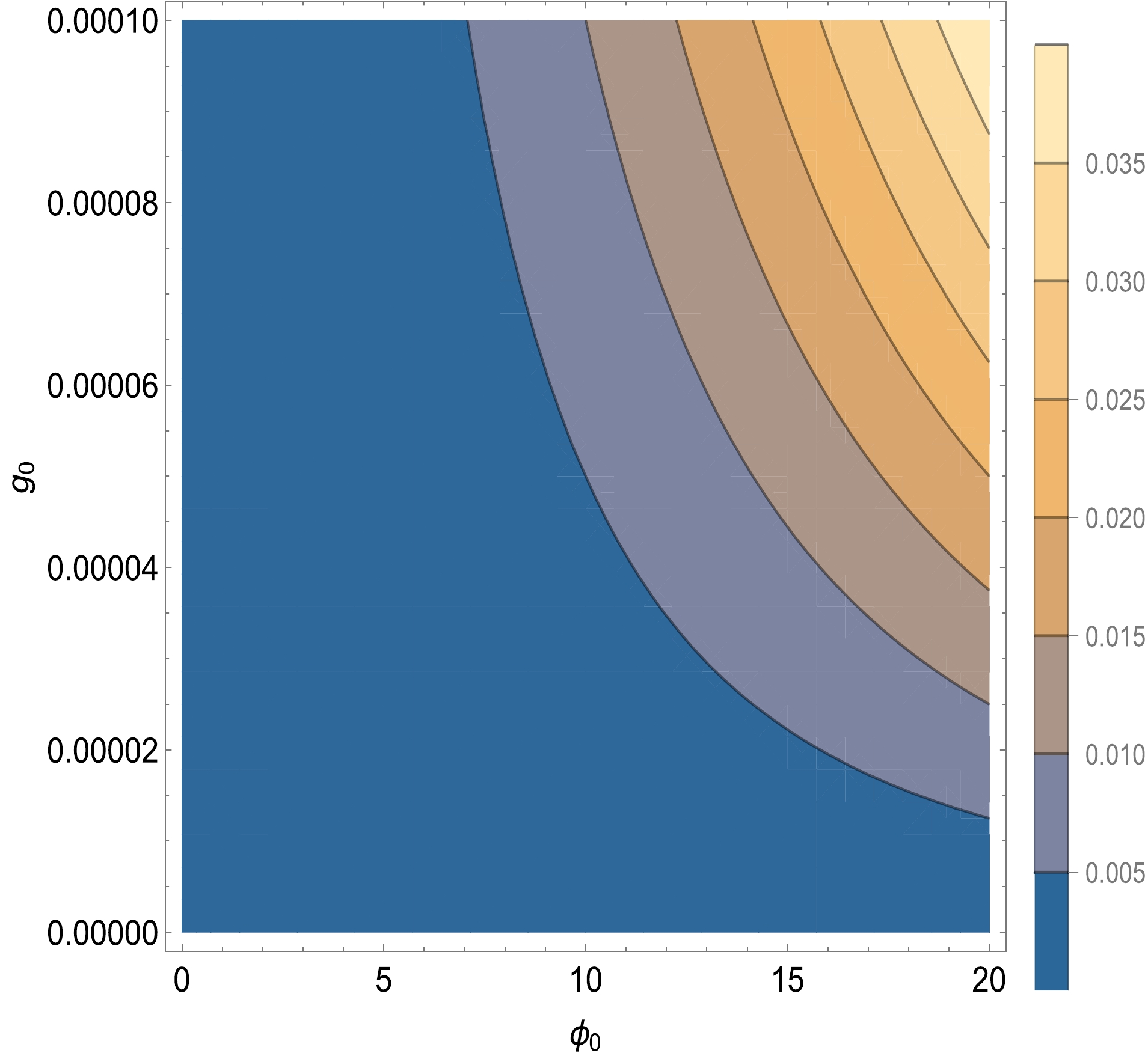
Figure 3. (color online) Contour plot of
$ q_k $ using Eq. (9): The horizontal line corresponds to the amplitude of inflaton, whose range is$0\leqslant \phi_0\leqslant20$ , determined by an e-folding number of approximately$ 60 $ . The vertical line denotes the value of$ g_0 $ , the range of which is from$ 0 $ to$ 0.0001 $ . We set$ M_{\rm P}=1 $ and$ a=1 $ . The right panel matches the value of$ q_k $ to its corresponding color.In this section, we thoroughly investigate the formation of PBHs during the preheating period. The key process in generating PBHs is utilizing the instability of the Mathieu equation characterized by δ functions in the power spectrum at small scales. In the next section, we study the equation of state (
$ EoS $ ) to investigate the DE epoch. -
The curvaton mechanism occurs during the preheating period and originates from the decay of the inflaton. Action (1) indicates that the main contribution disappears as the inflaton finishes the decay process. To clarify this situation, we construct a plot of potential consisting of the inflaton and curvaton; however, the curvaton arises from the transfer of the energy of the inflaton, and there are numerous uncertainties in the preheating mechanism. We only show the varying values of the inflaton and curvaton, for which the inflaton field is decreased and the curvaton is enhanced.
In Fig. 4, we show the potential of the curvaton during preheating, which is considered an illustration of the range of the curvaton. The field value of the curvaton originates from inflaton decay. Consequently, its contour plot is probably different from Fig. 4; however, the range of the curvaton field will not change. The range of the curvaton is of the order of
$ 10^{-15} $ in Planck units, taking proper parameters, which means that its energy density is dominant after inflaton decay but considerably smaller than the energy scope of the inflationary potential (matching the curvaton assumption). Moreover, the curvaton decay nearly disappears with the completion of inflaton decay, only keeping the relic of the exponential potential of the$\rm curvaton$ . In other words, it is almost impossible to decay into other particles determined by its effective mass$m_{\rm eff}^2=\dfrac{{\rm d}^2V(\chi)}{{\rm d}\chi^2}$ becausethe effective mass of the curvaton is of the order of the cosmological constant. Hence, the effective mass of the curvaton is considerably smaller than all types of fundamental particles, including Higgs particles, fermions, and gauge field particles. Therefore, in our model, the lifetime of the curvaton is almost the same as that of the inflaton because the main mass part of the curvaton is proportional to the inflationary potential. A simple and explicit analysis of the curvaton potential is considered, which naturally approaches a constant of the order of the cosmological constant, dubbed as the role of DE.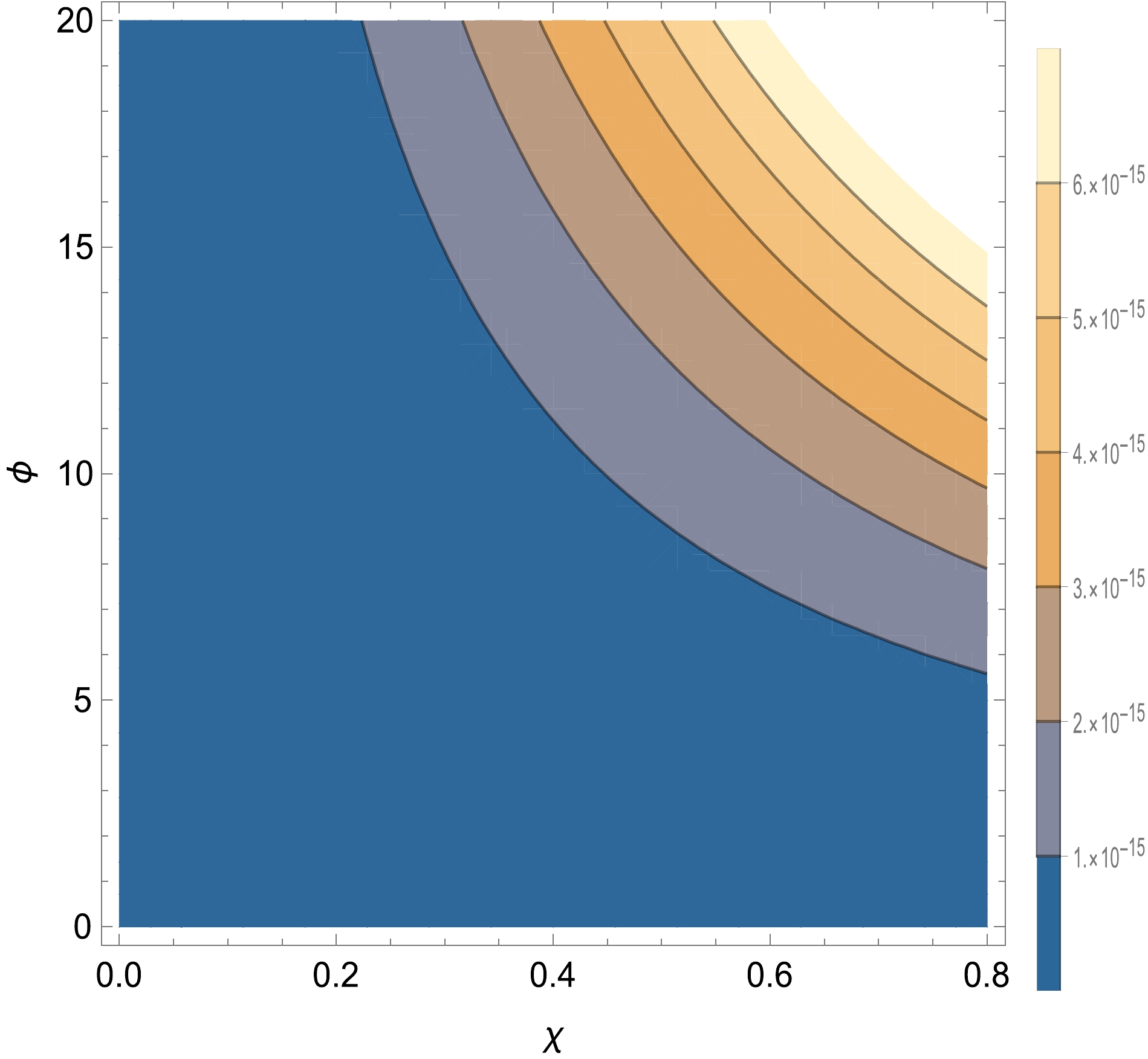
Figure 4. (color online) Contour plot of the curvaton. The potential of the curvaton field, in which
$ V(\chi)=\frac{g_0\chi^2}{M_{\rm P}}V(\phi)+ $ $ \lambda_0\exp(-\lambda_1\frac{\chi}{M_{\rm P}}) $ , where$ V(\phi)=\frac{1}{2}m^2\phi^2 $ as an example. We set$ M_{\rm P}=1 $ and$ g_0=0.001 $ , and$ \lambda_1 $ is absorbed in the curvaton field.In this section, we give a simple analysis that shows that the range of the curvaton is less than
$ 10^{-15} $ in Planck units. In this scope, the potential of the curvaton is dominant during preheating but considerably smaller than the inflationary energy scale, matching the assumption of the curvaton. At late times, the curvaton field also decays into other fundamental particles. However, there is a relic of the exponential potential of the curvaton, which plays a role in the cosmological constant, which can be dubbed as the DE dominating the current epoch. To some extent, this curvaton mechanism with the formation of PBHs during preheating may unify DE and DM. -
In this paper, we investigate the formation of PBHs during the preheating period using the instability of the Mathieu equation. In contrast with previous studies [78, 94, 95], we implement the running mass of the curvaton, which is proportional to (2), to investigate the formation of PBHs during the deeply preheating period (induced by the second inflation). Thus, the mass of the curvaton varies from COBE normalization to the DE scale determined by
$V_{\rm eff}=\dfrac{{\rm d}^2V}{{\rm d}\chi^2}$ as the inflaton finishes the decay. Owing to its large range, we can relate the exponential growth of curvature perturbation to the mass scale, which is the instability band corresponding to$ \tilde{k} $ . Then, we can adapt the property using δ functions, and the other energy scale is almost scale-invariant, as shown in Eq. (12). Thus, the simple analytical power spectrum perfectly agrees with observations, the details of which are shown in Fig. 1.Once this key result is obtained, we numerically simulate the abundance of PBHs among DM. Figure 2 clearly indicates the value of
$ f_{\rm PBH} $ with several specific values of mass corresponding to certain$ \tilde{k} $ . Here, we only use the property of the Lyapunov index to find the various corresponding values of k, which can simulate different values of$ f_{\rm PBH} $ because we choose proper parameters. Especially for Case$ 1 $ in Fig. 2, the value of the abundance of PBHs can reach$ 75\ $ % of DM, which may account for DM. During the preheating period, we show that the potential is of the order of$ 10^{-15} $ , dominating the main content of the Universe and consistent with the assumption of the curvaton. At late times, as the inflaton almost completes the decay process (curvaton disappears), there is a relic of the curvaton exponential potential that is dubbed as the role of dark energy, as illustrated in Sec. IV. Thus, our model may unify DE and DM.Our model is highly relevant to the coupling structure. Consequently, we could use this similar mechanism to explore the possibility of Higgs field formation during preheating, and the mass of the Higgs field is stringently constrained by the observation and its rich decay channels. This sheds light on Higgs physics exploration. Finally, we should emphasize that our non-Gaussianity parameter can be extended to a new parameter associated with w (EoS) and
$ r_{\rm decay} $ [96]. -
We are grateful for discussions with Diego Cruces on the value of δ and the numerical simulation of Wu-Long Xu.
Primordial black hole from the running curvaton
- Received Date: 2022-02-12
- Available Online: 2023-01-15
Abstract: In light of our previous study [Chin. Phys. C 44(8), 085103 (2020)], we investigate the possibility of the formation of a primordial black hole in the second inflationary process induced by the oscillation of the curvaton. By adopting the instability of the Mathieu equation, one can utilize the δ function to fully describe the power spectrum. Owing to the running of the curvaton mass, we can simulate the value of the abundance of primordial black holes covering almost all of the mass ranges. Three special cases are given. One case may account for dark matter because the abundance of a primordial black hole is approximately 75% . As late times, the relic of exponential potential may be approximated to a constant of the order of a cosmological constant, which is dubbed as the role of dark energy. Thus, our model could unify dark energy and dark matter from the perspective of phenomenology. Finally, it sheds new light on exploring Higgs physics.


 DownLoad: