


 Abstract
 HTML
HTML Reference
 Related
 PDF
PDF


-
The standard model (SM) has provided powerful descriptions of elementary particle physics and can explain most experiments with high precision [1]. However, it has been challenged by several experiments in recent years, for example, by
$ (g-2)_{\mu} $ [2, 3] and B decay anomalies [4]. Recently, the CDF collaboration announced a measurement of W boson mass [5], which was seven standard deviations heavier than the SM prediction. On the one hand, we are yet to scrutinize the theoretical and experimental uncertainties [6]. On the other hand, this may be a signature of new physics [7]. Currently, there are many studies dedicated to explaining this CDF anomaly [8–74].To explain the W mass anomaly, we can introduce new fermions and scalars. Vector-like quarks (VLQs) are well motivated in many new physics models, such as composite Higgs models [75, 76], little Higgs models [77, 78], grand unified theories [79], and extra dimension models [80]. From the viewpoint of model building, one attractive reason is that VLQs can avoid the problem of the quantum anomaly. In contrast, the leptoquarks (LQs) are well motivated in the grand unified theories [81–83]. LQs can be the solution to the
$ (g-2)_{\mu} $ , B physics, and other flavor anomalies [4, 84]. If we consider the VLQ and scalar LQ simultaneously, there can be two sources of W mass corrections. Furthermore, it is also possible to explain$ (g-2)_{\mu} $ at the same time. Here, we study the triplet LQ and triplet VLQ extended model.In this paper, we first construct the model in Sec. II. In Sec. III, we calculate the new physics contributions to the W boson mass and
$ (g-2)_{\mu} $ . Then, we perform the numerical analysis in Sec. IV. Finally, we present our summary and conclusions in Sec. V. -
The SM gauge group is
$ SU_C(3)\otimes SU_L(2)\otimes U_Y(1) $ . New particles can then carry different representations under this group. There are typically six types of scalar LQs [84, 85] and seven types of VLQs [86]. In our previous paper [87], we considered the$ S_3 $ LQ and$ (X,T,B)_{L,R} $ VLQ extended model to explain$ (g-2)_{\mu} $ ahead of the CDF W mass anomaly. Here, we investigate this model again, which is referred to as$ S_3+(X,T,B)_{L,R} $ for convenience.The representation of
$ S_3 $ is$ (\bar{3},3,1/3) $ , which is$ (3,3,2/3) $ for$ (X,T,B)_{L,R} $ ①. Then, the relevant Lagrangian can be decomposed as$\mathcal{L}_H^{\rm Yukawa}+\mathcal{L}_{S_3}^{\rm Yukawa}+\mathcal{L}_{XTB}^{\rm gauge}+ \mathcal{L}_{S_3}^{\rm gauge}+ \mathcal{L}_{S_3}^{\rm scalar}$ . Here,$\mathcal{L}_H^{\rm Yukawa}$ ,$\;\mathcal{L}_{S_3}^{\rm Yukawa}$ ,$\;\mathcal{L}_{XTB}^{\rm gauge}$ ,$\;\mathcal{L}_{S_3}^{\rm gauge}$ , and$\;\mathcal{L}_{S_3}^{\rm scalar}$ mark the VLQ Yukawa interactions with Higgs, VLQ Yukawa interactions with LQs, VLQ gauge interactions, LQ gauge interactions, and LQ scalar sector interactions, respectively. Below, we study these interactions carefully. -
First, let us express the Yukawa interactions with Higgs.
$ \begin{aligned}[b] \mathcal{L}\supset &-M_T\overline{(X,T,B)_L}\left(\begin{array}{c}X\\T\\B\end{array}\right)_{R}-y_{ij}^u\overline{Q_L}^iu_R^j\widetilde{\phi}\\&-y_{ij}^d\overline{Q_L}^id_R^j\phi-y_{iT}\overline{(Q_L)}^i\Psi_R\widetilde{\phi}+\mathrm{h.c.}. \end{aligned} $

(1) Here, we define
$\widetilde{\phi}\equiv {\rm i}\sigma^2\phi^{\ast}$ , and$ \sigma^a(a=1,2,3) $ are the Pauli matrices. The SM Higgs doublet ϕ is parameterized as$ \phi=[0,(v+h)/{\sqrt{2}}]^T $ in the unitary gauge.$Q_L^i,\;u_R^i,\;d_R^i$ represent the SM quark fields, and the triplet$ (X,T,B)_{L,R} $ can be parameterized in the following form:$ \begin{align} \Psi_{L,R}\equiv\Big(\begin{array}{cc}T_{L,R}&\sqrt{2}X_{L,R}\\ \sqrt{2}B_{L,R}&-T_{L,R}\end{array}\Big). \end{align} $

(2) For simplicity, we only consider the mixing between the third generation and VLQ [86, 91, 92]. After electroweak symmetry breaking (EWSB), we obtain the following mass terms:
$ \begin{aligned}[b] \mathcal{L}_{\rm mass}\supset - \left[\begin{array}{cc} \bar{t}_L&\bar{T}_L \end{array}\right] \left[\begin{array}{cc}\dfrac{1}{\sqrt{2}}y^u_{33}v&\dfrac{1}{\sqrt{2}}y_{3T}v\\ 0 &M_T\end{array}\right] \left[\begin{array}{cc} t_R\\T_R \end{array}\right] \end{aligned} $

$ \begin{aligned}[b] \quad- \left[\begin{array}{cc} \bar{b}_L&\bar{B}_L \end{array}\right] \left[\begin{array}{cc}\dfrac{1}{\sqrt{2}}y^d_{33}v&y_{3T}v\\ 0 &M_T\end{array}\right] \left[\begin{array}{cc} b_R\\B_R \end{array}\right]+\mathrm{h.c.}\; . \end{aligned} $

(3) Then, we can rotate the quark fields into mass eigenstates through the following transformations:
$ \begin{aligned}[b]& \left[\begin{array}{c}t_L\\T_L\end{array}\right]\rightarrow \left[\begin{array}{cc}\cos\theta_L^t&\sin\theta_L^t\\-\sin\theta_L^t&\cos\theta_L^t\end{array}\right] \left[\begin{array}{c}t_L\\T_L\end{array}\right],\quad\\& \left[\begin{array}{c}t_R\\T_R\end{array}\right]\rightarrow \left[\begin{array}{cc}\cos\theta_R^t&\sin\theta_R^t\\-\sin\theta_R^t&\cos\theta_R^t\end{array}\right] \left[\begin{array}{c}t_R\\T_R\end{array}\right], \end{aligned} $

(4) and
$ \begin{aligned}[b] & \left[\begin{array}{c}b_L\\B_L\end{array}\right]\rightarrow \left[\begin{array}{cc}\cos\theta_L^b&\sin\theta_L^b\\-\sin\theta_L^b&\cos\theta_L^b\end{array}\right] \left[\begin{array}{c}b_L\\B_L\end{array}\right],\quad \\& \left[\begin{array}{c}b_R\\B_R\end{array}\right]\rightarrow \left[\begin{array}{cc}\cos\theta_R^b&\sin\theta_R^b\\-\sin\theta_R^b&\cos\theta_R^b\end{array}\right] \left[\begin{array}{c}b_R\\B_R\end{array}\right]. \end{aligned} $

(5) After the above quark transformations, we have thefollowing mass eigenstate Yukawa interactions withHiggs:
$ \begin{aligned}[b]\\[-8pt] \mathcal{L}_H^{\rm Yukawa}\supset &-\frac{m_t}{v}(c_L^t)^2h\bar{t}t-\frac{m_T}{v}(s_L^t)^2h\bar{T}T-\frac{m_b}{v}(c_L^b)^2h\bar{b}b-\frac{m_B}{v}(s_L^b)^2h\bar{B}B-\frac{m_T}{v}s_L^tc_L^th(\bar{t}_LT_R+\bar{T}_Rt_L) \\ &-\frac{m_t}{v}s_L^tc_L^th(\bar{T}_Lt_R+\bar{t}_RT_L)-\frac{m_B}{v}s_L^bc_L^bh(\bar{b}_LB_R+\bar{B}_Rb_L)-\frac{m_b}{v}s_L^bc_L^bh(\bar{B}_Lb_R+\bar{b}_RB_L). \end{aligned} $ 
(6) In the above, the physical masses are labeled as
$m_{t,~T,~b,~B}$ .$s_L^{t(b)},~\;c_L^{t(b)},~\;s_R^{t(b)},~\;c_R^{t(b)}$ represent$\sin\theta_L^{t(b)}, \cos\theta_L^{t(b)},~\sin\theta_R^{t(b)}, ~\cos\theta_R^{t(b)}$ , respectively. Moreover, we have the following relations:$ \begin{aligned}[b] \tan\theta_R^t=&\frac{m_t}{m_T}\tan\theta_L^t,\; M_T^2=m_T^2(c_L^t)^2+m_t^2(s_L^t)^2,\\ \tan\theta_R^b=&\frac{m_b}{m_B}\tan\theta_L^b,\; M_T^2=m_B^2(c_L^b)^2+m_b^2(s_L^b)^2,\\ \sin2\theta_L^b=&\frac{\sqrt{2}(m_T^2-m_t^2)}{m_B^2-m_b^2}\sin2\theta_L^t. \end{aligned} $

(7) Hence, there are two new independent input parameters
$ m_T $ and$ \theta_L^t $ (also denoted as$ \theta_L $ in the following), and the parameters$M_T,\;m_B,\;\theta_R^t,\;\theta_L^b,\;\theta_R^b$ can be determined from the above equations (see App. A). One interesting point is that the mass of the X quark is$ M_T $ , which is less than$ m_T $ and$ m_B $ . -
Now, let us consider the Yukawa interactions with LQs. In this
$ S_3+(X,T,B)_{L,R} $ model, gauge eigenstate interactions can be written as$ \begin{align} \mathcal{L}\supset x_{ij}\overline{(Q_L)^C}^{i,a}({\rm i}\sigma^2)^{ab}(S_3)^{bc}L_L^{j,c}+x_{Ti} \mathrm{Tr}[\overline{(\Psi_R)^C}S_3]e_R^i+\mathrm{h.c.}. \end{align} $

(8) Here,
$ L_L^i,e_R^i $ denote the SM lepton fields. Similarly, we also parameterize the$ S_3 $ triplet in the following form:$ \begin{align} S_3\equiv\Big(\begin{array}{cc}S_3^{1/3}&\sqrt{2}S_3^{4/3}\\ \sqrt{2}S_3^{-2/3}&-S_3^{1/3}\end{array}\Big). \end{align} $

(9) In the above, the matrix elements
$ \big(\overline{(\Psi_R)^C}\big)_{ij} $ are defined as$ \overline{\big((\Psi_R)_{ij}\big)^C} $ . After EWSB, the related Lagrangian can be reparameterized as$ \begin{aligned}[b] & \mathcal{L}\supset y_L^{S_3\mu T}\bar{\mu}\; \omega_-\; T^C(S_3^{1/3})^\ast+y_R^{S_3\mu t}\bar{\mu}\; \omega_+\; t^C(S_3^{1/3})^\ast+y_L^{S_3\mu T}\bar{\mu}\; \omega_-\; B^C(S_3^{4/3})^\ast+\sqrt{2}y_R^{S_3\mu t}\bar{\mu}\; \omega_+\; b^C(S_3^{4/3})^\ast\\ &\quad+y_L^{S_3\mu T}\bar{\mu}\; \omega_-\; X^C(S_3^{-2/3})^\ast-\sqrt{2}y_R^{S_3\mu t}\overline{(\nu_{\mu})_L}\; \omega_+\; t^C(S_3^{-2/3})^\ast+y_R^{S_3\mu t}\overline{(\nu_{\mu})_L}\; \omega_+\; b^C(S_3^{1/3})^\ast+\mathrm{h.c.}. \end{aligned} $

(10) Here,
$ \omega_\pm $ are the chirality operators$ (1\pm\gamma^5)/2 $ . The new parameters$ y_L^{S_3\mu T} $ and$ y_R^{S_3\mu t} $ can be determined from the original$ x_{ij} $ and$ x_{Ti} $ . We adopt the new parameters for convenience. When performing the transformations in Eqs. (4) and (5), we have the following mass eigenstate Yukawa interactions with LQs:$ \begin{aligned}[b]\\[-8pt] \mathcal{L}_{S^3}^{\rm Yukawa} &\supset\bar{\mu}(-y_L^{S_3\mu T}s_R^t\omega_-+y_R^{S_3\mu t}c_L^t\omega_+)t^C(S_3^{1/3})^\ast+\bar{\mu}(y_L^{S_3\mu T}c_R^t\omega_-+y_R^{S_3\mu t}s_L^t\omega_+)T^C(S_3^{1/3})^\ast\\ & +\bar{\mu}(-y_L^{S_3\mu T}s_R^b\omega_-+\sqrt{2}y_R^{S_3\mu t}c_L^b\omega_+)b^C(S_3^{4/3})^\ast+\bar{\mu}(y_L^{S_3\mu T}c_R^b\omega_-+\sqrt{2}y_R^{S_3\mu t}s_L^b\omega_+)B^C(S_3^{4/3})^\ast\\ & -\sqrt{2}y_R^{S_3\mu t}\overline{(\nu_{\mu})_L}\; \omega_+(c_L^tt^C+s_L^tT^C)(S_3^{-2/3})^\ast+y_R^{S_3\mu t}\overline{(\nu_{\mu})_L}\; \omega_+\; (c_L^bb^C+s_L^bB^C)(S_3^{1/3})^\ast\\ & +y_L^{S_3\mu T}\bar{\mu}\; \omega_-\; X^C(S_3^{-2/3})^\ast+\mathrm{h.c.}. \end{aligned} $ 
(11) -
For the tripet VLQ Ψ, the covariant derivative of the electroweak part is defined as
$D_{\mu}\Psi=\partial_{\mu}\Psi- {\rm i}g[W_{\mu}^a\tau^a,\Psi]- {\rm i}g^{\prime}YB_{\mu}\Psi$ , with Y as the$ U_Y(1) $ charge.$ W_{\mu}^a $ and$ B_{\mu} $ label the$ SU(2)_L $ and$ U_Y(1) $ gauge fields, respectively. The gauge interactions are written as$\mathrm{Tr}(\bar{\Psi}{\rm i}\not D\Psi)/2$ , in which the factor$ 1/2 $ is to normalize the kinetic terms. After EWSB, the charged current interactions can be written as$ \begin{align} \mathcal{L}\supset gW_{\mu}^+(\overline{T_L}\gamma^{\mu}B_L+\overline{T_R}\gamma^{\mu}B_R-\overline{X_L}\gamma^{\mu}T_L-\overline{X_R}\gamma^{\mu}T_R)+\mathrm{h.c.}. \end{align} $

(12) Here,
$ W_{\mu}^\pm $ is defined as$(W_{\mu}^1\mp {\rm i}W_{\mu}^2)/\sqrt{2}$ . For the neutral current interactions, we perform the rotations$ W_{\mu}^3= \cos\theta_W Z_{\mu}+\sin\theta_W A_{\mu} $ and$ B_{\mu}=\cos\theta_W A_{\mu}-\sin\theta_W Z_{\mu} $ , in which$ \theta_W $ is the Weinberg angle. For convenience,$ \sin\theta_W(\cos\theta_W) $ is abbreviated as$ s_W(c_W) $ . Thus, the neutral current interactions can be written as$ \begin{aligned}[b] & \mathcal{L}\supset\frac{g}{c_W}(-\frac{2}{3}s_W^2)Z_{\mu}(\overline{T_L}\gamma^{\mu}T_L+\overline{T_R}\gamma^{\mu}T_R)+\frac{g}{c_W}(-1+\frac{1}{3}s_W^2)Z_{\mu}(\overline{B_L}\gamma^{\mu}B_L+\overline{B_R}\gamma^{\mu}B_R)\\ &\quad+\frac{g}{c_W}(1-\frac{5}{3}s_W^2)(\overline{X_L}\gamma^{\mu}X_L+\overline{X_R}\gamma^{\mu}X_R).\\ \end{aligned} $ 
(13) As we know, third generation quarks interact with W and Z bosons in the following form:
$ \begin{aligned}[b] & \mathcal{L}\supset \frac{g}{\sqrt{2}}W_{\mu}^+(\overline{t_L}\gamma^{\mu}b_L+\mathrm{h.c.})+\frac{g}{c_W}Z_{\mu}[(\frac{1}{2}-\frac{2}{3}s_W^2)\overline{t_L}\gamma^{\mu}t_L-\frac{2}{3}s_W^2\overline{t_R}\gamma^{\mu}t_R]\\ &\quad+\frac{g}{c_W}Z_{\mu}[(-\frac{1}{2}+\frac{1}{3}s_W^2)\overline{b_L}\gamma^{\mu}b_L+\frac{1}{3}s_W^2\overline{b_R}\gamma^{\mu}b_R]. \end{aligned} $

(14) After rotating the quark fields with Eqs. (4) and (5), we have following mass eigenstate charged current interactions②:
$ \begin{aligned}[b] \mathcal{L}_{XTB}^{\rm gauge}& \supset\frac{g}{\sqrt{2}}W_{\mu}^+\Big\{\bar{t}\gamma^{\mu}[(c_L^tc_L^b+\sqrt{2}s_L^ts_L^b)\omega_-+\sqrt{2}s_R^ts_R^b\omega_+]b+\bar{t}\gamma^{\mu}[(c_L^ts_L^b-\sqrt{2}s_L^tc_L^b)\omega_--\sqrt{2}s_R^tc_R^b\omega_+]B\\ & +\bar{T}\gamma^{\mu}[(s_L^tc_L^b-\sqrt{2}c_L^ts_L^b)\omega_--\sqrt{2}c_R^ts_R^b\omega_+]b+\bar{T}\gamma^{\mu}[(s_L^ts_L^b+\sqrt{2}c_L^tc_L^b)\omega_-+\sqrt{2}c_R^tc_R^b\omega_+]B\Big\}\\ & +gW_{\mu}^+[\overline{X_L}\gamma^{\mu}(s_L^tt_L-c_L^tT_L)+\overline{X_R}\gamma^{\mu}(s_R^tt_R-c_R^tT_R)]+\mathrm{h.c.}. \end{aligned} $

(15) Similarly, we have the following mass eigenstate neutral current interactions:
$ \begin{aligned}[b] \mathcal{L}_{XTB}^{\rm gauge}&\supset\frac{g}{2c_W}Z_{\mu}\Big\{\bar{t}\gamma^{\mu}[\big((c_L^t)^2-\frac{4}{3}s_W^2\big)\omega_--\frac{4}{3}s_W^2\omega_+]t+\bar{T}\gamma^{\mu}[\big((s_L^t)^2-\frac{4}{3}s_W^2\big)\omega_--\frac{4}{3}s_W^2\omega_+]T\\ & +s_L^tc_L^t(\overline{t_L}\gamma^{\mu}T_L+\overline{T_L}\gamma^{\mu}t_L)]+\bar{b}\gamma^{\mu}[\big(-1-(s_L^b)^2+\frac{2}{3}s_W^2\big)\omega_-+\big(-2(s_R^b)^2+\frac{2}{3}s_W^2\big)\omega_+]b\\ & +\bar{B}\gamma^{\mu}[(-1-(c_L^b)^2+\frac{2}{3}s_W^2)\omega_-+\big(-2(c_R^b)^2+\frac{2}{3}s_W^2\big)\omega_+]B+s_L^bc_L^b(\overline{b_L}\gamma^{\mu}B_L+\overline{B_L}\gamma^{\mu}b_L)\\ & +2s_R^bc_R^b(\overline{b_R}\gamma^{\mu}B_R+\overline{B_R}\gamma^{\mu}b_R)+2(1-\frac{5}{3}s_W^2)(\overline{X_L}\gamma^{\mu}X_L+\overline{X_R}\gamma^{\mu}X_R)\Big\}. \end{aligned} $

(16) -
For the LQ
$ S_3 $ , the covariant derivative of the electroweak part is defined as$D_{\mu}S_3=\partial_{\mu}S_3-{\rm i}g[W_{\mu}^a\tau^a,S_3]- {\rm i}g^{\prime}YB_{\mu}S_3$ . Then, the gauge interactions$\mathcal{L}_{S_3}^{\rm gauge}\supset \dfrac{1}{2} \mathrm{Tr}[(D_{\mu}S_3)^{\dagger}(D^{\mu}S_3)]$ can be expanded as shown below.●
$ S_3S_3W $ interaction:$ \begin{align} {\rm i}gW_{\mu}^+\Big[(\partial^{\mu}S_3^{4/3})^{\ast}S_3^{1/3}-(\partial^{\mu}S_3^{1/3})(S_3^{4/3})^{\ast}+(\partial^{\mu}S_3^{-2/3})(S_3^{1/3})^{\ast}-(\partial^{\mu}S_3^{1/3})^{\ast}S_3^{-2/3}\Big]+\mathrm{h.c.}. \end{align} $

(17) ●
$ S_3S_3Z $ interaction:$ \begin{aligned}[b] &\frac{{\rm i}gZ_{\mu}}{c_W}\Bigg\{-\frac{1}{3}s_W^2\Big[(\partial^{\mu}S_3^{1/3})(S_3^{1/3})^{\ast}-(\partial^{\mu}S_3^{1/3})^{\ast}S_3^{1/3}\Big]+\left(\frac{2}{3}s_W^2-1\right)\Big[(\partial^{\mu}S_3^{-2/3})(S_3^{-2/3})^{\ast}-(\partial^{\mu}S_3^{-2/3})^{\ast}S_3^{-2/3}\Big]\\ &\quad+\left(1-\frac{4}{3}s_W^2\right)\Big[(\partial^{\mu}S_3^{4/3})(S_3^{4/3})^{\ast}-(\partial^{\mu}S_3^{4/3})^{\ast}S_3^{4/3}\Big]\Bigg\}. \end{aligned} $

(18) ●
$ S_3S_3\gamma $ interaction:$ \begin{aligned}[b] &{\rm i}eA_{\mu}\Bigg\{\frac{1}{3}\Big[(\partial^{\mu}S_3^{1/3})(S_3^{1/3})^{\ast}-(\partial^{\mu}S_3^{1/3})^{\ast}S_3^{1/3}\Big]-\frac{2}{3}\Big[(\partial^{\mu}S_3^{-2/3})(S_3^{-2/3})^{\ast}-(\partial^{\mu}S_3^{-2/3})^{\ast}S_3^{-2/3}\Big]\\ &\quad+\frac{4}{3}\Big[(\partial^{\mu}S_3^{4/3})(S_3^{4/3})^{\ast}-(\partial^{\mu}S_3^{4/3})^{\ast}S_3^{4/3}\Big]\Bigg\}. \end{aligned} $

(19) ●
$ S_3S_3WW $ interaction:$ \begin{align} g^2\Big\{W_{\mu}^+W^{-,{\mu}}\Big[2S_3^{1/3}(S_3^{1/3})^{\ast}+S_3^{-2/3}(S_3^{-2/3})^{\ast}+S_3^{4/3}(S_3^{4/3})^{\ast}\Big]-S_3^{4/3}(S_3^{-2/3})^{\ast}W_{\mu}^-W^{-,{\mu}}-S_3^{-2/3}(S_3^{4/3})^{\ast}W_{\mu}^+W^{+,{\mu}}\Big\}. \end{align} $

(20) ●
$ S_3S_3WZ $ interaction:$ \begin{align} \frac{g^2}{c_W}W_{\mu}^+Z^{\mu}\left[\left(-1+\frac{1}{3}s_W^2\right)S_3^{-2/3}(S_3^{1/3})^{\ast}+\left(-1+\frac{5}{3}s_W^2\right)S_3^{1/3}(S_3^{4/3})^{\ast}\right]+\mathrm{h.c.}. \end{align} $

(21) ●
$ S_3S_3W\gamma $ interaction:$ \begin{align} egW_{\mu}^+A^{\mu}\left[-\frac{1}{3}S_3^{-2/3}\Big(S_3^{1/3}\Big)^{\ast}-\frac{5}{3}S_3^{1/3}\Big(S_3^{4/3}\Big)^{\ast}\right]+\mathrm{h.c.}. \end{align} $

(22) ●
$ S_3S_3ZZ $ interaction:$ \begin{align} \frac{g^2}{c_W^2}Z_{\mu}Z^{\mu}\left[\frac{1}{9}s_W^4S_3^{1/3}(S_3^{1/3})^{\ast}+\left(1-\frac{4}{3}s_W^2\right)^2S_3^{4/3}(S_3^{4/3})^{\ast}+\left(1-\frac{2}{3}s_W^2\right)^2S_3^{-2/3}(S_3^{-2/3})^{\ast}\right]. \end{align} $

(23) ●
$ S_3S_3Z\gamma $ interaction:$ \begin{align} \frac{2eg}{c_W}Z_{\mu}A^{\mu}\left[-\frac{1}{9}s_W^2S_3^{1/3}(S_3^{1/3})^{\ast}+\frac{4}{3}\left(1-\frac{4}{3}s_W^2\right)S_3^{4/3}(S_3^{4/3})^{\ast}-\frac{2}{3}\left(-1+\frac{2}{3}s_W^2\right)S_3^{-2/3}(S_3^{-2/3})^{\ast}\right]. \end{align} $

(24) ●
$ S_3S_3\gamma\gamma $ interaction:$ \begin{align} e^2A_{\mu}A^{\mu}\left[\frac{1}{9}S_3^{1/3}(S_3^{1/3})^{\ast}+\frac{16}{9}S_3^{4/3}(S_3^{4/3})^{\ast}+\frac{4}{9}S_3^{-2/3}(S_3^{-2/3})^{\ast}\right]. \end{align} $

(25) -
Here, we consider the scalar sector interactions. The mass related terms can be written as③
$ \begin{aligned}[b] &\mathcal{L}_{S_3}^{\rm scalar}\supset-\frac{1}{2}m_{S_3}^2 \mathrm{Tr}[(S_3)^{\dagger}S_3]-\lambda_{\phi S_3}(\phi^{\dagger}\phi) \mathrm{Tr}[(S_3)^{\dagger}S_3]\\&\quad-\widetilde{\lambda}_{\phi S_3}\phi^{\dagger}(S_3)^{\dagger}S_3\phi. \end{aligned} $

(26) After EWSB, we have the following mass equations [93]:
$ \begin{aligned}[b] m_{S_3^{4/3}}^2=&m_{S_3}^2+\lambda_{\phi S_3}v^2+\widetilde{\lambda}_{\phi S_3}v^2,\quad\\ m_{S_3^{1/3}}^2=&m_{S_3}^2+\lambda_{\phi S_3}v^2+\frac{1}{2}\widetilde{\lambda}_{\phi S_3}v^2,\quad m_{S_3^{-2/3}}^2=m_{S_3}^2+\lambda_{\phi S_3}v^2. \end{aligned} $

(27) Obviously, the
$ (\phi^{\dagger}\phi) \mathrm{Tr}[(S_3)^{\dagger}S_3] $ term does not contribute to the mass splittings. Meanwhile, there are tree level generated mass splittings, which are controlled by the coupling$ \widetilde{\lambda}_{\phi S_3} $ . In fact, this is similar to the traditional colorless electroweak triplet. The difference is that the mass splittings for the traditional electroweak triplet can also be caused by the non-zero triplet vacuum expectation value [94, 95]. In Ref. [96], the authors studied the mass splittings originating from the$ S_1 $ and$ S_3 $ LQ mixing.Although there are three mass parameters,
$ m_{S_3^{4/3}}^2 $ ,$ m_{S_3^{1/3}}^2 $ , and$ m_{S_3^{-2/3}}^2 $ , only two of them are relevant because we can redefine the mass. For convenience, let us define the following mass splitting quantity:$ \begin{align} \Delta m^2(\approx 2m_{S_3^{1/3}}\cdot\Delta m)\equiv m_{S_3^{4/3}}^2-m_{S_3^{1/3}}^2=m_{S_3^{1/3}}^2-m_{S_3^{-2/3}}^2=\frac{1}{2}\widetilde{\lambda}_{\phi S_3}v^2. \end{align} $

(28) Thus, we can choose the input parameters to be
$ (m_{S_3^{1/3}},\widetilde{\lambda}_{\phi S_3}) $ or$ (m_{S_3^{1/3}},\Delta m) $ . -
If we choose the
$ \{\alpha,G_F,m_Z\} $ scheme, the W boson mass can be determined from the formula [97, 98]$ \begin{align} m_W^2=\frac{m_Z^2}{2}\Bigg(1+\sqrt{1-\frac{\sqrt{8}\pi\alpha(1+\Delta r)}{G_Fm_Z^2}}\Bigg), \end{align} $

(29) and then we have the following approximation:
$ \begin{align} \frac{\Delta m_W^2}{m_W^2}=-\frac{s_W^2}{c_W^2-s_W^2}\delta r. \end{align} $

(30) In the above, we define the quantities
$\Delta m_W^2\equiv (m_W^{ \mathrm{NP}})^2-$ $ (m_W^{ \mathrm{SM}})^2 $ and$ \delta r\equiv\Delta r^{ \mathrm{NP}}-\Delta r^{ \mathrm{SM}} $ to isolate the new physics contributions. If we neglect the new physics contributions from the wave function renormalization constants, vertex, and box diagrams in μ decay④, the W mass correction can be correlated with the$S,\;T,\;U$ oblique parameters as [99–104]$ \begin{align} \frac{\Delta m_W^2}{m_W^2}=\frac{2\Delta m_W}{m_W}=\frac{\alpha}{c_W^2-s_W^2}(-\frac{1}{2}\Delta S+c_W^2\Delta T+\frac{c_W^2-s_W^2}{4s_W^2}\Delta U), \end{align} $

(31) where we define the deviations
$ \Delta S\equiv S^{ \mathrm{NP}}-S^{ \mathrm{SM}} $ ,$ \Delta T\equiv T^{ \mathrm{NP}} -T^{ \mathrm{SM}} $ , and$ \Delta U\equiv U^{ \mathrm{NP}}-U^{ \mathrm{SM}} $ . In most cases, the T parameter dominates. There are mainly two contributions to the oblique parameters in the$ S_3+(X,T,B)_{L,R} $ model. One is from the LQ contributions, and the other is from the VLQs.Now, let us turn to the oblique contributions from the LQ loops, which are denoted as
$ \Delta S^{S_3} $ ,$ \Delta T^{S_3} $ , and$ \Delta U^{S_3} $ . Unlike the traditional electroweak Higgs triplet model,$ S_3 $ does not modify the T parameter at tree level because of the exact color symmetry. The complete one-loop results can be calculated through the interactions given in Sec. II.D, and the details are given in App. B. The U parameter formula is lengthy, and the S and T parameters have the following compact expressions:$ \begin{aligned}[b] \Delta S^{S_3}=&-\frac{N_C}{9\pi}\log\frac{m_{S_3^{4/3}}^2}{m_{S_3^{-2/3}}^2},\\\Delta T^{S_3}=&\frac{N_C}{8\pi m_W^2s_W^2}[\theta_+(m_{S_3^{4/3}}^2,m_{S_3^{1/3}}^2)+\theta_+(m_{S_3^{-2/3}}^2,m_{S_3^{1/3}}^2)]. \end{aligned} $

(32) Here,
$ N_C=3 $ is a color factor, and the function$ \theta_+ $ is defined as$ \begin{align} \theta_+(y_1,y_2)\equiv y_1+y_2-\frac{2y_1y_2}{y_1-y_2}\log\frac{y_1}{y_2}. \end{align} $

(33) Obviously, we have
$ \Delta T^{S_3}\ge0 $ because of the inequality$ \theta_+(x,y)\ge0 $ , in which the equality applies if and only if$ x=y $ . For$ \Delta S^{S_3} $ , it is negative if$ m_{S_3^{4/3}}>m_{S_3^{-2/3}} $ ($ \widetilde{\lambda}_{\phi S_3}>0 $ ) and positive if$ m_{S_3^{4/3}}<m_{S_3^{-2/3}} $ ($ \widetilde{\lambda}_{\phi S_3}<0 $ ). The mass expressions are shown in Eqs. (27) and (28). In the approximation of$ \widetilde{\lambda}_{\phi S_3}v^2\ll m_{S_3^{1/3}}^2 $ (or$ \Delta m\ll m_{S_3^{1/3}} $ ), the S, T, and U parameters can be expanded as$ \begin{aligned}[b]\Delta S^{S_3}\approx & -\frac{\widetilde{\lambda}_{\phi S_3}v^2}{3\pi m_{S_3^{1/3}}^2}\approx-\frac{4\Delta m}{3\pi m_{S_3^{1/3}}},\\ \Delta T^{S_3}\approx & \frac{(\widetilde{\lambda}_{\phi S_3})^2v^4}{16\pi s_W^2m_W^2m_{S_3^{1/3}}^2}\approx\frac{(\Delta m)^2}{\pi s_W^2m_W^2},\\\Delta U^{S_3}\approx & \frac{7(\widetilde{\lambda}_{\phi S_3})^2v^4}{40\pi m_{S_3^{1/3}}^4}\approx\frac{14(\Delta m)^2}{5\pi m_{S_3^{1/3}}^2}. \end{aligned} $

(34) In the limit
$ \widetilde{\lambda}_{\phi S_3}\rightarrow0 $ , they will vanish. These results completely agree with those in Refs. [105, 106].For the VLQ part, the oblique corrections are caused by both the modification of SM quark gauge couplings and new VLQ loops, which are denoted as
$ \Delta S^{XTB} $ ,$ \Delta T^{XTB} $ , and$ \Delta U^{XTB} $ . Their analytic expressions are lengthy; hence, the details are given in App. C. Considering$ m_b\ll m_t\ll m_T $ and$ s_L^t\ll1 $ , the formulae can be approximated as$ \begin{aligned}[b]\Delta S^{XTB}\approx & \frac{N_C(s_L^t)^2}{18\pi}(-12\log\frac{m_T}{m_t}-16\log\frac{m_t}{m_b}+29),\\ \Delta T^{XTB}\approx &\frac{N_Cm_t^2(s_L^t)^2}{8\pi s_W^2m_W^2}(6\log\frac{m_T}{m_t}-5),\\\Delta U^{XTB}\approx &\frac{N_C(s_L^t)^2}{18\pi}(24\log\frac{m_t}{m_b}-5). \end{aligned} $

(35) If
$ s_L^t $ goes to zero,$ \Delta S^{XTB} $ ,$ \Delta T^{XTB} $ , and$ \Delta U^{XTB} $ will vanish. Our expansion results agree with those in Cao's paper [90], whereas the expansion of the S parameter differs from the result in Ref. [107]⑤. According to Eq. (35),$ \Delta T^{XTB} $ and$ \Delta U^{XTB} $ are always positive, whereas$ \Delta S^{XTB} $ is always negative. Typically,$ \Delta T^{XTB} $ is several times larger than$ \Delta S^{XTB} $ and$ \Delta U^{XTB} $ because of the$ m_t^2/(m_W^2s_W^2) $ factor.After summing the fermion and boson contributions, we can obtain the total oblique parameter deviations as
$ \Delta S\equiv\Delta S^{XTB}+\Delta S^{S_3} $ ,$ \Delta T\equiv\Delta T^{XTB}+\Delta T^{S_3} $ , and$\Delta U\equiv \Delta U^{XTB}+ \Delta U^{S_3}$ . To explain the W boson mass anomaly, a positive$ \Delta T $ is required, which is satisfied for both the VLQ and LQ contributions. There are four independent parameters involved in the oblique corrections:$ m_T $ and$ s_L $ for the VLQ, and$ m_{S_3^{1/3}} $ and$ \widetilde{\lambda}_{\phi S_3} $ for the LQ. -
According to the BNL and FNAL experiments [2, 3], the most recent muon anomalous magnetic dipole moment was measured as
$ a_{\mu}^{ \mathrm{Exp}}=116592061(41)\times10^{-11} $ . In the SM, it is predicted as$ a_{\mu}^{ \mathrm{SM}}=116591810(43)\times10^{-11} $ [109]. Thus, the deviation is$ \Delta a_{\mu}\equiv a_{\mu}^{ \mathrm{Exp}}-a_{\mu}^{ \mathrm{SM}}= (251\pm59)\times 10^{-11} $ , which corresponds to a$ 4.2\sigma $ discrepancy. LQ models can be the solution to this$ (g-2)_{\mu} $ anomaly [84, 105, 110–115]. In our previous paper [87], we studied$ (g-2)_{\mu} $ in the$ S_3+(X,T,B)_{L,R} $ model, in which the contributions are mainly from T and B quarks. Considering all contributions from$t,\;T,\;b,\;B,\;X$ quarks, the complete expression is calculated as$ \begin{aligned}[b] \Delta a_{\mu}=&\frac{m_{\mu}^2}{8\pi^2}\Bigg\{\frac{|y_L^{S_3\mu T}|^2(s_R^t)^2+|y_R^{S_3\mu t}|^2(c_L^t)^2}{m_{S_3^{1/3}}^2}f_{LL}^{S_3}(\frac{m_t^2}{m_{S_3^{1/3}}^2})-\frac{2m_t}{m_{\mu}}\frac{c_L^ts_R^t}{m_{S_3^{1/3}}^2} \mathrm{Re}[y_L^{S_3\mu T}(y_R^{S_3\mu t})^\ast]f_{LR}^{S_3}(\frac{m_t^2}{m_{S_3^{1/3}}^2})\\ &+\frac{|y_L^{S_3\mu T}|^2(c_R^t)^2+|y_R^{S_3\mu t}|^2(s_L^t)^2}{m_{S_3^{1/3}}^2}f_{LL}^{S_3}(\frac{m_T^2}{m_{S_3^{1/3}}^2})+\frac{2m_T}{m_{\mu}}\frac{s_L^tc_R^t}{m_{S_3^{1/3}}^2} \mathrm{Re}[y_L^{S_3\mu T}(y_R^{S_3\mu t})^\ast]f_{LR}^{S_3}(\frac{m_T^2}{m_{S_3^{1/3}}^2})\\ &+\frac{|y_L^{S_3\mu T}|^2(s_R^b)^2+2|y_R^{S_3\mu t}|^2(c_L^b)^2}{m_{S_3^{4/3}}^2}\widetilde{f}_{LL}^{S_3}(\frac{m_b^2}{m_{S_3^{4/3}}^2})-\frac{2\sqrt{2}m_b}{m_{\mu}}\frac{c_L^bs_R^b}{m_{S_3^{4/3}}^2} \mathrm{Re}[y_L^{S_3\mu T}(y_R^{S_3\mu t})^\ast]\widetilde{f}_{LR}^{S_3}(\frac{m_b^2}{m_{S_3^{4/3}}^2})\\ &+\frac{|y_L^{S_3\mu T}|^2(c_R^b)^2+2|y_R^{S_3\mu t}|^2(s_L^b)^2}{m_{S_3^{4/3}}^2}\widetilde{f}_{LL}^{S_3}(\frac{m_B^2}{m_{S_3^{4/3}}^2})+\frac{2\sqrt{2}m_B}{m_{\mu}}\frac{s_L^bc_R^b}{m_{S_3^{4/3}}^2} \mathrm{Re}[y_L^{S_3\mu T}(y_R^{S_3\mu t})^\ast]\widetilde{f}_{LR}^{S_3}(\frac{m_B^2}{m_{S_3^{4/3}}^2}) +\frac{|y_L^{S_3\mu T}|^2}{m_{S_3^{-2/3}}^2}\hat{f}_{LL}^{S_3}(\frac{m_X^2}{m_{S_3^{-2/3}}^2})\Bigg\}. \end{aligned} $

(36) In the above, the subscripts "
$ LL $ " and "$ LR $ " denote the contributions without and with chiral enhancements. The related functions are defined as$ \begin{aligned}[b] f_{LL}^{S_3}(x)\equiv &\frac{1+4x-5x^2+2x(2+x)\log x}{4(1-x)^4},\\ f_{LR}^{S_3}(x)\equiv &-\frac{7-8x+x^2+(4+2x)\log x}{4(1-x)^3},\\ \widetilde{f}_{LL}^{S_3}(x)\equiv&-\frac{2-7x+2x^2+3x^3+2x(1-4x)\log x}{4(1-x)^4},\\\widetilde{f}_{LR}^{S_3}(x)\equiv&-\frac{1+4x-5x^2-(2-8x)\log x}{4(1-x)^3},\\ \hat{f}_{LL}^{S_3}(x)\equiv&\frac{4+x-8x^2+3x^3+2x(5-2x)\log x}{4(1-x)^4}. \end{aligned} $

(37) Considering
$ m_b\ll m_t\ll m_T\approx m_B $ ,$ \theta_L^t\ll1 $ , and$ m_{S_3^{4/3}}\approx m_{S_3^{1/3}}\approx m_{S_3^{-2/3}}\approx m_{S_3} $ , it can be approximated as$ \begin{aligned}[b] \Delta a_{\mu}\approx&\frac{m_{\mu}m_T}{4\pi^2m_{S_3}^2}[f_{LR}^{S_3}(\frac{m_T^2}{m_{S_3}^2})+2\widetilde{f}_{LR}^{S_3}(\frac{m_T^2}{m_{S_3}^2})\\&+\frac{m_t^2}{m_T^2}(\frac{7}{4}+\log \frac{m_t^2}{m_{S_3}^2})]\cdot \mathrm{Re}[y_L^{S_3\mu T}(y_R^{S_3\mu t})^\ast]s_L. \end{aligned} $

(38) As we can see, the contributions to
$ (g-2)_{\mu} $ are mainly determined by the parameters$ m_T $ ,$ s_L $ , and$ m_{S_3^{1/3}} $ . Although the parameter$ \widetilde{\lambda}_{\phi S_3} $ can also alter the correction, it is sub-dominated through the LQ mass differences. -
In this paper, we choose the SM input parameters to be
$m_Z=91.1876\;\mathrm{GeV},m_W=80.379\;\mathrm {GeV},m_{\mu}=105.66\;\mathrm{MeV}, m_t=172.5\;\mathrm{GeV}, m_b=4.2\;\mathrm{GeV},\alpha=1/128$ , and$ c_W=m_W/m_Z $ [1]. Furthermore, we define the W mass deviation quantity$ \Delta m_W^{ \mathrm{exp}}\equiv m_W^{ \mathrm{exp}}-m_W^{ \mathrm{SM}} $ . Here,$ m_W^{ \mathrm{exp}} $ is the CDF result$80,433.5\,\pm9.4 \;\mathrm{MeV}$ [5], and$ m_W^{ \mathrm{SM}} $ is the SM prediction$80,357\pm6 \;\mathrm{MeV}$ [1]. Then,$ \Delta m_W^{ \mathrm{exp}} $ is calculated to be$76.5\pm11.2 \;\mathrm{MeV}$ . For the VLQ mass, the direct search requires it to be above 1.4 TeV [116, 117]. For the LQ mass, the direct search also requires it to be above 1.5 TeV [118, 119]. We also consider the constraints from electro-weak precision observables. Because it is small for the correlation between the oblique corrections and$ Zbb $ couplings [120, 121], we can treat them separately for simplicity. There is a$ b-B $ mixing induced tree level modification of the$ Zbb $ coupling, which leads to the bound$ s_L\lesssim0.05 $ [86, 107]. In Ref. [122], the oblique parameters are updated as follows (standard average scenario):$ \begin{align} \Delta S^{ \mathrm{fit}}=0.005,\quad\sigma_S=0.096,\quad\Delta T^{ \mathrm{fit}}=0.040,\quad\sigma_T=0.120,\\\ \quad\Delta U^{ \mathrm{fit}}=0.134,\quad\sigma_U=0.087, \end{align} $

(39) with the correlation matrix
$ \begin{align} \rho=\left[\begin{array}{ccc} 1.00 & 0.91 & -0.65 \\ 0.91 & 1.00 & -0.88 \\ -0.65 & -0.88 & 1.00 \end{array}\right]. \end{align} $

(40) Then, we can define the
$ \chi^2 $ quantity as$ \begin{align} \chi^2\equiv\sum\limits_{i,j=1,2,3}\frac{O_i-O_i^{ \mathrm{fit}}}{\sigma_i}(\rho^{-1})_{ij}\frac{O_j-O_j^{ \mathrm{fit}}}{\sigma_j}, \end{align} $

(41) where the indices
$1,\;2,\;3$ label the$S,\;T,\;U$ parameters. Next, we perform the$ \chi^2 $ fit of the oblique parameters.First, let us roughly compare the contributions from
$ (X,T,B)_{L,R} $ and$ S_3 $ . In Fig. 1, we show their individual contributions to the W boson mass. For the pure$ (X,T,B)_{L,R} $ case, the behavior is as expected because we have the approximation$ \Delta m_W\propto (s_L^t)^2\log(m_T/m_t) $ . Thus, we need larger$ s_L^t $ and$ m_T $ to produce a sizable W mass correction. For the pure$ S_3 $ case, the behaviour is also as expected because we have the approximation$ \Delta m_W\propto (\widetilde{\lambda}_{\phi S_3})^2/m_{S_3^{1/3}}^2 $ if$ \widetilde{\lambda}_{\phi S_3}\sim \mathcal{O}(1) $ . Thus, we need larger$ \widetilde{\lambda}_{\phi S_3} $ and small$ m_{S_3^{1/3}} $ to produce a sizable W mass correction. In Fig. 2, we show the parameter space allowed by the CDF W mass measurement and the oblique parameters. For the pure$ (X,T,B)_{L,R} $ case, we find that$ m_T $ should be at least 3.8 TeV when$ s_L=0.05 $ . For the pure$ S_3 $ case, we find that$ |\widetilde{\lambda}_{\phi S_3}| $ should be at least 2.3 when$m_{S_3^{1/3}}=1.5\;\mathrm{TeV}$ .$ |\Delta m| $ lies at approximately 25 GeV, which is almost independent of$ m_{S_3^{1/3}} $ ⑥.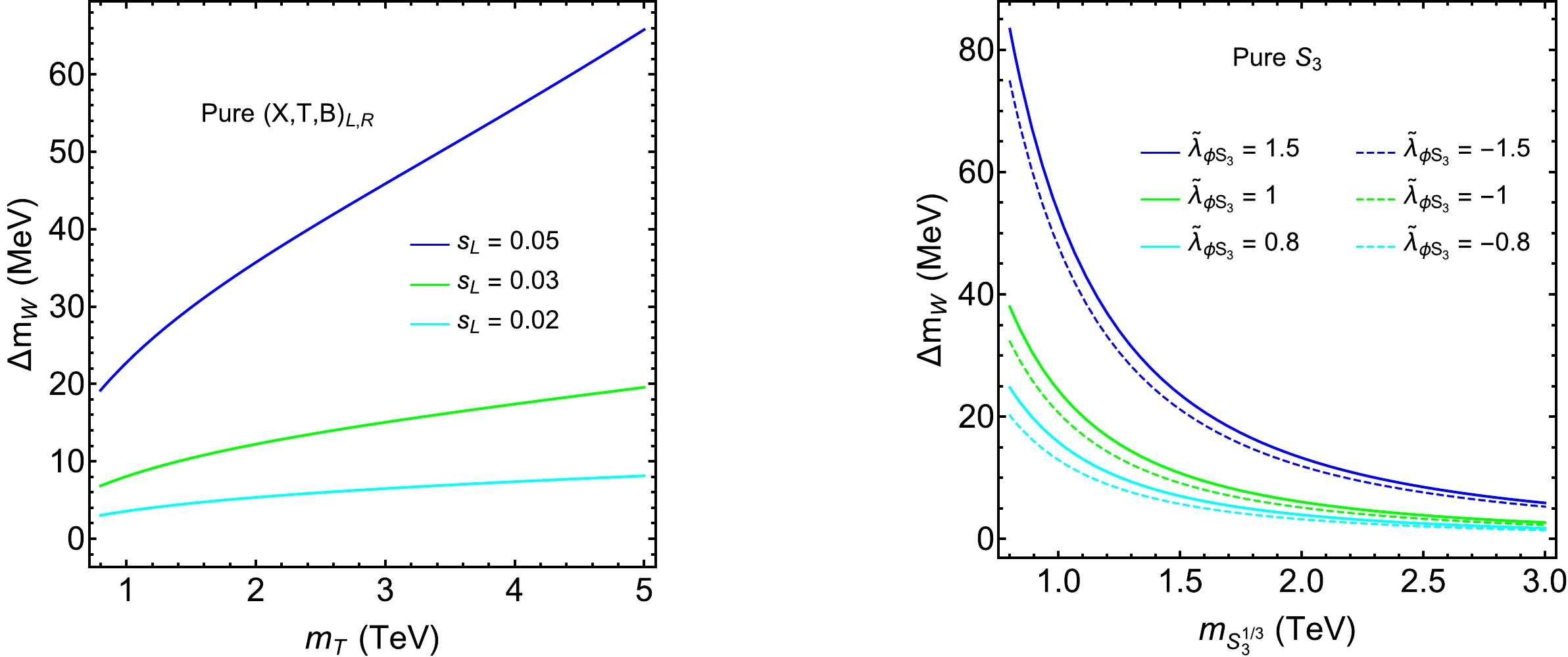
Figure 1. (color online) Pure
$ (X,T,B)_{L,R} $ contributions to$ \Delta m_W $ as a function of$ m_T $ for different$ s_L $ (left). The pure$ S_3 $ contributions to$ \Delta m_W $ as a function of$ m_{S_3^{1/3}} $ for different$ \widetilde{\lambda}_{\phi S_3} $ (right).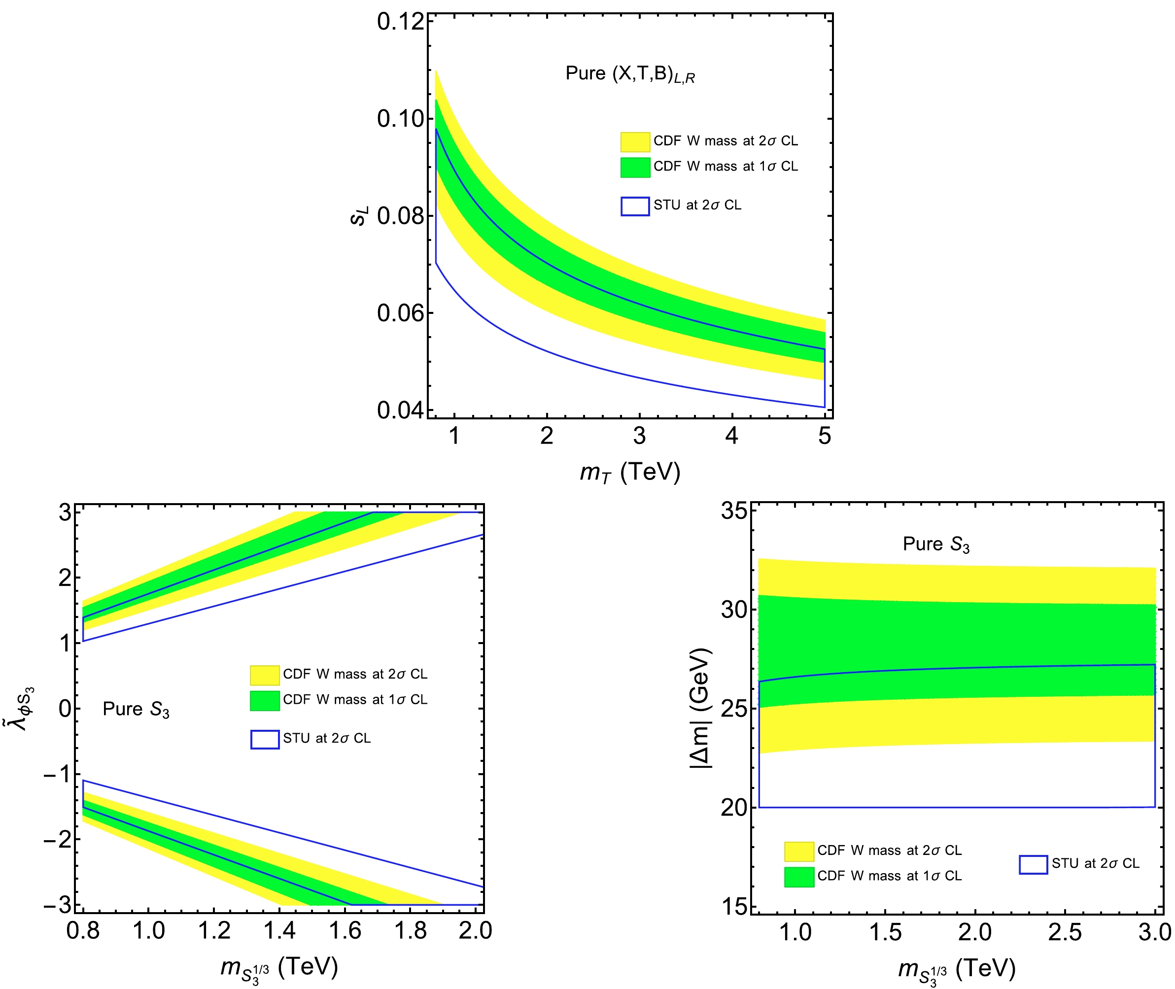
Figure 2. (color online) Pure
$ (X,T,B)_{L,R} $ case in the plane of$ m_T-s_L $ (upper), the pure$ S_3 $ case in the plane of$ m_{S_3^{1/3}}-\widetilde{\lambda}_{\phi S_3} $ (lower left), and the pure$ S_3 $ case in the plane of$ m_{S_3^{1/3}}-|\Delta m| $ (lower right). The CDF W mass allowed parameter space is shown at the$ 1\sigma $ (green) and$ 2\sigma $ (yellow) confidence levels (CLs), respectively. The blue line enclosed area is bounded by the$ S,T,U $ parameters at the$ 2\sigma $ CL.In Fig. 3, we consider the contributions from
$ (X,T,B)_{L,R} $ and$ S_3 $ at the same time. In the two plots above, we show the W mass allowed regions in the plane of$m_T-s_L$ with fixed$ m_{S_3^{1/3}} $ and$ \widetilde{\lambda}_{\phi S_3} $ . For the scenarios$m_{S_3^{1/3}}=$ 1.5 TeV and$ \widetilde{\lambda}_{\phi S_3}=0.8,1 $ , we find that the lower limit of$ m_T $ can be decreased to 3.1 TeV and 2.7 TeV when$ s_L=0.05 $ . In the two plots below, we show the W mass allowed regions in the plane of$m_{S_3^{1/3}}-\widetilde{\lambda}_{\phi S_3}$ with fixed$ m_T $ and$ s_L $ . For the scenario$ s_L=0.05 $ and$m_T=3 \;\mathrm{TeV}$ , we find that the lower limit of$ |\widetilde{\lambda}_{\phi S_3}| $ can be decreased to 0.9 when$m_{S_3^{1/3}}=1.5 \;\mathrm{TeV}$ . For the scenario$ s_L=0.05 $ and$m_T=5 \,\mathrm{TeV}$ ,$ \widetilde{\lambda}_{\phi S_3} $ can be zero because pure$ (X,T,B)_{L,R} $ is sufficient to produce the W mass correction.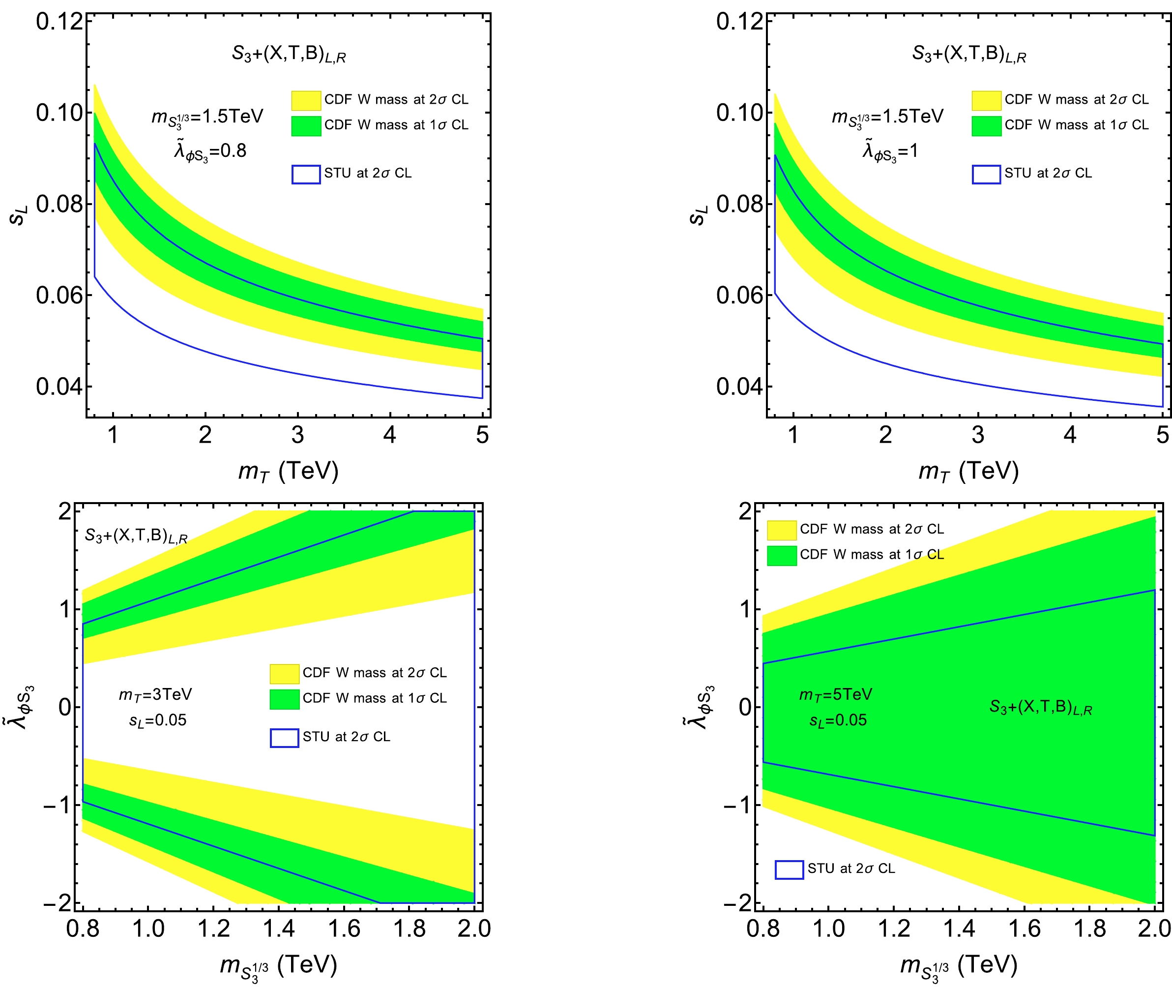
Figure 3. (color online) CDF W mass allowed regions in the plane of
$ m_T-s_L $ for the scenarios$m_{S_3^{1/3}}=1.5\, \mathrm{TeV},\widetilde{\lambda}_{\phi S_3}=0.8$ (upper left), and$m_{S_3^{1/3}}=1.5 \,\mathrm{TeV},\widetilde{\lambda}_{\phi S_3}=1$ (upper right). The CDF W mass allowed regions in the plane of$ m_{S_3^{1/3}}-\widetilde{\lambda}_{\phi S_3} $ for the scenarios$m_T=3 \,\mathrm{TeV},s_L=0.05$ (lower left), and$m_T=5 \,\mathrm{TeV},s_L=0.05$ (lower right). The blue line enclosed area is bounded by the$ S,T,U $ parameters at the$ 2\sigma $ CL.Moreover, the
$ S_3+(X,T,B)_{L,R} $ model can also explain the$ (g-2)_{\mu} $ anomaly. In our previous paper [87], we took the LQs to have the same mass ($ \widetilde{\lambda}_{\phi S_3}=0 $ ). Here, we consider the LQ mass differences, which only lead to small effects. Based on the previous W mass numerical analysis, we choose two benchmark points$m_T=3 ~\mathrm{TeV}, s_L=0.05, ~m_{S_3^{1/3}}=1.5 ~\mathrm{TeV},~ \widetilde{\lambda}_{\phi S_3}=1$ and$m_T=5 ~\mathrm{TeV}, s_L= 0.05,~m_{S_3^{1/3}}=1.5 ~\mathrm{TeV},~\widetilde{\lambda}_{\phi S_3}=0$ . Under the first benchmark point, the leading order numerical result of$ \Delta a_{\mu} $ is$ -0.5914\times10^{-7} \mathrm{Re}[y_L^{S_3\mu T}(y_R^{S_3\mu t})^\ast] $ , which constrains$ \mathrm{Re}[y_L^{S_3\mu T}(y_R^{S_3\mu t})^\ast] $ to be roughly in the ranges$ (-0.052, -0.032) $ and$ (-0.062,-0.022) $ at the$ 1\sigma $ and$ 2\sigma $ CLs, respectively. Under the second benchmark point, the leading order numerical result of$ \Delta a_{\mu} $ is$-0.4542\times 10^{-7} \times \mathrm{Re}[y_L^{S_3\mu T}(y_R^{S_3\mu t})^\ast]$ , which constrains$ \mathrm{Re}[y_L^{S_3\mu T}(y_R^{S_3\mu t})^\ast] $ to be roughly in the ranges$ (-0.068,-0.042) $ and$(-0.081, -0.029)$ at the$ 1\sigma $ and$ 2\sigma $ CLs, respectively. In Fig. 4, we show the regions allowed by$ (g-2)_{\mu} $ in the plane of$ y_L^{S_3\mu T}-y_R^{S_3\mu t} $ .
Figure 4. (color online) Regions allowed by
$ (g-2)_{\mu} $ at the$ 1\sigma $ (green) and$ 2\sigma $ (yellow) CLs, respectively. Here, we include the full contributions besides the chirally enhanced parts. -
We consider the
$ (X,T,B)_{L,R} $ and$ S_3 $ extended model to explain the W boson mass anomaly. The mass splittings of VLQs originate from mixing with SM quarks, and the mass splittings of LQs can be generated through interaction with SM Higgs. For VLQ oblique parameter corrections, some papers adopt the existing formulae directly without any examination, which are based on the singlet and doublet properties. In this paper, we obtain the complete VLQ and LQ contributions to the S, T, and U parameters. As we know, direct search experiments push the VLQ and LQ mass lower limits to approximately TeV. We also consider the constraints from electroweak precision measurements, of which$ Zbb $ coupling imposes the strong bound$ s_L\lesssim0.05 $ . For the pure$ (X,T,B)_{L,R} $ model,$ m_T $ should be as heavy as 4 TeV for$ s_L=0.05 $ . For the pure$ S_3 $ model,$ |\widetilde{\lambda}_{\phi S_3}|\sim2 $ is required for$m_{S_3^{1/3}}= 1.5 \,\mathrm{TeV}$ . For the$ S_3+(X,T,B)_{L,R} $ model, we find that the W boson mass and$ (g-2)_{\mu} $ anomalies can be explained simultaneously. Because W mass corrections can be shared by the VLQ and LQ, they allow for lower$ m_T $ and smaller$ |\widetilde{\lambda}_{\phi S_3}| $ . Depending on the choice of$ m_T,s_L,m_{S_3^{1/3}} $ , the$ (g-2)_{\mu} $ anomaly can also be explained when$ \mathrm{Re}[y_L^{S_3\mu T}(y_R^{S_3\mu t})^\ast] $ ranges from$ \sim \mathcal{O}(-0.1) $ to$ \mathcal{O}(-0.01) $ . -
We are grateful for the W mass seminar held by the "All Things EFT committee" and the seminar held in China (https://indico.ihep.ac.cn/event/16155), from which we benefited a lot. We also thank Hiroshi Okada, Junjie Cao, Haiying Cai, and Rui Zhang for helpful discussions.
-
Relations between the VLQ parameters:
$ \begin{aligned}[b] \tan\theta_R^t=&\frac{m_t}{m_T}\tan\theta_L^t,\\\tan\theta_R^b=&\frac{m_b}{m_B}\tan\theta_L^b,\\\sin2\theta_L^b=&\frac{\sqrt{2}(m_T^2-m_t^2)}{m_B^2-m_b^2}\sin2\theta_L^t,\\ M_T^2=& m_T^2(c_L^t)^2+m_t^2(s_L^t)^2=m_B^2(c_L^b)^2+m_b^2(s_L^b)^2,\\ M_T=&m_Tc_L^tc_R^t+m_ts_L^ts_R^t=m_Bc_L^bc_R^b+m_bs_L^bs_R^b=\frac{m_ts_L^t}{s_R^t}\\=&\frac{m_Tc_L^t}{c_R^t}=\frac{m_bs_L^b}{s_R^b}=\frac{m_Bc_L^b}{c_R^b},\\ &\sqrt{2}(m_Tc_R^ts_L^t-m_tc_L^ts_R^t)\\=&m_Bc_R^bs_L^b-m_bc_L^bs_R^b. \end{aligned}\tag{A1} $

From the approximations
$ m_b\ll m_t\ll m_T $ and$ s_L^t\ll1 $ , we obtain the following results:$ \begin{aligned}[b] \theta_R^t\approx& \frac{m_t}{m_T}\theta_L^t,\\m_X=&M_T\approx m_T\left[1-\frac{1}{2}\left(1-\frac{m_t^2}{m_T^2}\right)(\theta_L^t)^2\right],\\ \theta_L^b\approx & \frac{\sqrt{2}(m_T^2-m_t^2)}{m_T^2-m_b^2}\theta_L^t\approx\sqrt{2}\left(1-\frac{m_t^2}{m_T^2}\right)\theta_L^t,\\\theta_R^b\approx & \frac{\sqrt{2}m_b(m_T^2-m_t^2)}{m_T(m_T^2-m_b^2)}\theta_L^t\approx\frac{\sqrt{2}m_b}{m_T}\left(1-\frac{m_t^2}{m_T^2}\right)\theta_L^t,\\ m_B\approx &m_T\left[1+\frac{(m_T^2-m_t^2)(m_T^2-2m_t^2+m_b^2)}{2m_T^2(m_T^2-m_b^2)}(\theta_L^t)^2\right]\\\approx & m_T\left[1+\frac{1}{2}\left(1-\frac{m_t^2}{m_T^2}\right)\left(1-\frac{2m_t^2}{m_T^2}\right)(\theta_L^t)^2\right]. \end{aligned}\tag{A2} $

-
First, let us define the
$ B_0 $ function as$ B_0(p^2,m_1^2,m_2^2)\equiv\Delta_{\epsilon}-\int_0^1{\rm d}x\log\frac{xm_1^2+(1-x)m_2^2-x(1-x)p^2}{\mu^2}. \tag{B1} $

In the above,
$ \Delta_{\epsilon} $ is defined as$ 1/\epsilon-\gamma_E+\log4\pi $ . Here, we adopt the dimensional regularization, and$ D=4-2\epsilon $ is the space-time dimension.$ \gamma_E $ is Euler's constant, and μ is the renormalization scale.According to the LQ gauge interactions derived in Sec. II.D, the self energies of neutral gauge bosons are calculated as
$ \begin{aligned}[b] &\Pi_{\gamma\gamma}(p^2)=\frac{e^2N_C}{16\pi^2}\sum\limits_{S_3^i}Q_{S_3^i}^2[\frac{1}{3}(4m_{S_3^i}^2-p^2)B_0(p^2,m_{S_3^i}^2,m_{S_3^i}^2)-\frac{4}{3}m_{S_3^i}^2B_0(0,m_{S_3^i}^2,m_{S_3^i}^2)-\frac{2}{9}p^2],\\ &\Pi_{\gamma Z}(p^2)=\frac{egN_C}{16\pi^2c_W}\sum\limits_{S_3^i}Q_{S_3^i}(I_3^{S_3^i}-Q_{S_3^i}s_W^2)[\frac{1}{3}(4m_{S_3^i}^2-p^2)B_0(p^2,m_{S_3^i}^2,m_{S_3^i}^2)-\frac{4}{3}m_{S_3^i}^2B_0(0,m_{S_3^i}^2,m_{S_3^i}^2)-\frac{2}{9}p^2],\\ &\Pi_{ZZ}(p^2)=\frac{g^2N_C}{16\pi^2c_W^2}\sum\limits_{S_3^i}(I_3^{S_3^i}-Q_{S_3^i}s_W^2)^2[\frac{1}{3}(4m_{S_3^i}^2-p^2)B_0(p^2,m_{S_3^i}^2,m_{S_3^i}^2)-\frac{4}{3}m_{S_3^i}^2B_0(0,m_{S_3^i}^2,m_{S_3^i}^2)-\frac{2}{9}p^2],\\ \end{aligned} \tag{B2}$

where
$S_3^i=S_3^{4/3},~S_3^{1/3},~S_3^{-2/3}$ .$ Q_{S_3^i} $ and$ I_3^{S_3^i} $ denote their electric charge and the third component of weak isospin, which means$Q_{S_3^{4/3}}=4/3,~Q_{S_3^{1/3}}=1/3,~Q_{S_3^{-2/3}}=-2/3$ and$I_3^{S_3^{4/3}}=1,~I_3^{S_3^{1/3}}=0,~I_3^{S_3^{-2/3}}=-1$ .Then, the self energy of the W boson is calculated as
$ \begin{aligned}[b] \Pi_{WW}(p^2)=&\frac{g^2N_C}{16\pi^2}\Big\{-\frac{p^2}{9}[3B_0(p^2,m_{S_3^{4/3}}^2,m_{S_3^{1/3}}^2)+3B_0(p^2,m_{S_3^{-2/3}}^2,m_{S_3^{1/3}}^2)+4]\\ &+\frac{2}{3}[(m_{S_3^{4/3}}^2+m_{S_3^{1/3}}^2)B_0(p^2,m_{S_3^{4/3}}^2,m_{S_3^{1/3}}^2)+(m_{S_3^{-2/3}}^2+m_{S_3^{1/3}}^2)B_0(p^2,m_{S_3^{-2/3}}^2,m_{S_3^{1/3}}^2)\\ &-m_{S_3^{4/3}}^2B_0(0,m_{S_3^{4/3}}^2,m_{S_3^{4/3}}^2)-m_{S_3^{-2/3}}^2B_0(0,m_{S_3^{-2/3}}^2,m_{S_3^{-2/3}}^2)-2m_{S_3^{1/3}}^2B_0(0,m_{S_3^{1/3}}^2,m_{S_3^{1/3}}^2)]\\ &-\frac{1}{3p^2}[(m_{S_3^{4/3}}^2-m_{S_3^{1/3}}^2)^2B_0(p^2,m_{S_3^{4/3}}^2,m_{S_3^{1/3}}^2)+(m_{S_3^{-2/3}}^2-m_{S_3^{1/3}}^2)^2B_0(p^2,m_{S_3^{-2/3}}^2,m_{S_3^{1/3}}^2)\\ &-m_{S_3^{4/3}}^2(m_{S_3^{4/3}}^2-m_{S_3^{1/3}}^2)B_0(0,m_{S_3^{4/3}}^2,m_{S_3^{4/3}}^2)-m_{S_3^{-2/3}}^2(m_{S_3^{-2/3}}^2-m_{S_3^{1/3}}^2)B_0(0,m_{S_3^{-2/3}}^2,m_{S_3^{-2/3}}^2)\\ &+m_{S_3^{1/3}}^2(m_{S_3^{4/3}}^2+m_{S_3^{-2/3}}^2-2m_{S_3^{1/3}}^2)B_0(0,m_{S_3^{1/3}}^2,m_{S_3^{1/3}}^2)-(m_{S_3^{4/3}}^2-m_{S_3^{1/3}}^2)^2-(m_{S_3^{-2/3}}^2-m_{S_3^{1/3}}^2)^2]\Big\}. \end{aligned}\tag{B3} $

Based on the exact expressions of
$ \Pi_{VV}(p^2) $ , we can derive$ \Pi_{VV}(0) $ and$\Pi_{VV}'(0)\equiv {\rm d}\Pi_{VV}(p^2)/{\rm d}p^2|_{p^2=0}$ as follows:$ \begin{aligned}[b] \Pi_{\gamma\gamma}(0)=&\Pi_{\gamma Z}(0)=\Pi_{ZZ}(0)=0,\\ \Pi_{\gamma\gamma}'(0)=&-\frac{e^2N_C}{48\pi^2}\sum\limits_{S_3^i}Q_{S_3^i}^2(\Delta_{\epsilon}-\log\frac{m_{S_3^i}^2}{\mu^2}),\\ \Pi_{\gamma Z}'(0)=&-\frac{egN_C}{48\pi^2c_W}\sum\limits_{S_3^i}Q_{S_3^i}(I_3^{S_3^i}-Q_{S_3^i}s_W^2)(\Delta_{\epsilon}-\log\frac{m_{S_3^i}^2}{\mu^2}),\\ \Pi_{ZZ}'(0)=&-\frac{g^2N_C}{48\pi^2c_W^2}\sum\limits_{S_3^i}(I_3^{S_3^i}-Q_{S_3^i}s_W^2)^2(\Delta_{\epsilon}-\log\frac{m_{S_3^i}^2}{\mu^2}),\\ \Pi_{WW}(0)=&\frac{g^2N_C}{16\pi^2}[\frac{1}{2}(m_{S_3^{4/3}}^2+m_{S_3^{-2/3}}^2-2m_{S_3^{1/3}}^2)-\frac{m_{S_3^{1/3}}^2m_{S_3^{4/3}}^2}{m_{S_3^{1/3}}^2-m_{S_3^{4/3}}^2}\log\frac{m_{S_3^{1/3}}^2}{m_{S_3^{4/3}}^2}-\frac{m_{S_3^{1/3}}^2m_{S_3^{-2/3}}^2}{m_{S_3^{1/3}}^2-m_{S_3^{-2/3}}^2}\log\frac{m_{S_3^{1/3}}^2}{m_{S_3^{-2/3}}^2}],\\ \Pi_{WW}'(0)=&\frac{g^2N_C}{16\pi^2}[-\frac{2}{3}(\Delta_{\epsilon}-\log\frac{m_{S_3^{1/3}}^2}{\mu^2})-\frac{4}{9}-\frac{m_{S_3^{4/3}}^4+m_{S_3^{1/3}}^4-14m_{S_3^{4/3}}^2m_{S_3^{1/3}}^2}{18(m_{S_3^{4/3}}^2-m_{S_3^{1/3}}^2)^2}-\frac{m_{S_3^{-2/3}}^4+m_{S_3^{1/3}}^4-14m_{S_3^{-2/3}}^2m_{S_3^{1/3}}^2}{18(m_{S_3^{-2/3}}^2-m_{S_3^{1/3}}^2)^2}\\ &+\frac{m_{S_3^{4/3}}^4(m_{S_3^{4/3}}^2-3m_{S_3^{1/3}}^2)}{3(m_{S_3^{4/3}}^2-m_{S_3^{1/3}}^2)^3}\log\frac{m_{S_3^{4/3}}^2}{m_{S_3^{1/3}}^2}+\frac{m_{S_3^{-2/3}}^4(m_{S_3^{-2/3}}^2-3m_{S_3^{1/3}}^2)}{3(m_{S_3^{-2/3}}^2-m_{S_3^{1/3}}^2)^3}\log\frac{m_{S_3^{-2/3}}^2}{m_{S_3^{1/3}}^2}]. \end{aligned}\tag{B4} $

The S, T, and U parameters are defined as [99–101]
$ \begin{aligned}[b] \frac{\alpha S}{4s_W^2c_W^2}\equiv &\frac{\Pi_{ZZ}(m_Z^2)-\Pi_{ZZ}(0)}{m_Z^2}-\frac{c_W^2-s_W^2}{s_Wc_W}\Pi_{\gamma Z}'(0)-\Pi_{\gamma\gamma}'(0)=\Pi_{ZZ}'(0)-\frac{c_W^2-s_W^2}{s_Wc_W}\Pi_{\gamma Z}'(0)-\Pi_{\gamma\gamma}'(0),\\ \alpha T\equiv &\frac{\Pi_{WW}(0)}{m_W^2}-\frac{\Pi_{ZZ}(0)}{m_Z^2},\\ \frac{\alpha U}{4s_W^2}\equiv &\frac{\Pi_{WW}(m_W^2)-\Pi_{WW}(0)}{m_W^2}-c_W^2\frac{\Pi_{ZZ}(m_Z^2)-\Pi_{ZZ}(0)}{m_Z^2}-2s_Wc_W\Pi_{\gamma Z}'(0)-s_W^2\Pi_{\gamma\gamma}'(0)\\ =&\Pi_{WW}'(0)-c_W^2\Pi_{ZZ}'(0)-2s_Wc_W\Pi_{\gamma Z}'(0)-s_W^2\Pi_{\gamma\gamma}'(0). \end{aligned}\tag{B5} $

When we adopt Eq. (B4) in the above definitions, the LQ contributions to the S, T, and U parameters are calculated in the following explicit forms:
$ \begin{aligned}[b] \Delta S^{S_3}=&-\frac{N_c}{9\pi}\log\frac{m_{S_3^{4/3}}^2}{m_{S_3^{-2/3}}^2},\qquad \Delta T^{S_3}=\frac{N_c}{8\pi m_W^2s_W^2}[\theta_+(m_{S_3^{4/3}}^2,m_{S_3^{1/3}}^2)+\theta_+(m_{S_3^{-2/3}}^2,m_{S_3^{1/3}}^2)],\\ \Delta U^{S_3}=&\frac{N_C}{\pi}[-\frac{4}{9}-\frac{m_{S_3^{4/3}}^4+m_{S_3^{1/3}}^4-14m_{S_3^{4/3}}^2m_{S_3^{1/3}}^2}{18(m_{S_3^{4/3}}^2-m_{S_3^{1/3}}^2)^2}-\frac{m_{S_3^{-2/3}}^4+m_{S_3^{1/3}}^4-14m_{S_3^{-2/3}}^2m_{S_3^{1/3}}^2}{18(m_{S_3^{-2/3}}^2-m_{S_3^{1/3}}^2)^2}\\ &+\frac{m_{S_3^{1/3}}^4(-3m_{S_3^{4/3}}^2+m_{S_3^{1/3}}^2)}{3(m_{S_3^{4/3}}^2-m_{S_3^{1/3}}^2)^3}\log\frac{m_{S_3^{4/3}}^2}{m_{S_3^{1/3}}^2}+\frac{m_{S_3^{1/3}}^4(-3m_{S_3^{-2/3}}^2+m_{S_3^{1/3}}^2)}{3(m_{S_3^{-2/3}}^2-m_{S_3^{1/3}}^2)^3}\log\frac{m_{S_3^{-2/3}}^2}{m_{S_3^{1/3}}^2}]. \end{aligned}\tag{B6} $

As we can see, the divergence and scale μ are exactly canceled in the oblique parameters.
-
Because the triplet VLQ is involved, we cannot simply adopt the formulae of the S and T parameters in Ref. [108], in which some calculations are based on singlet and doublet properties. In this section, we present a detailed deduction.
Let us generally denote the quark interactions with gauge bosons
$ V_1 $ and$ V_2 $ as$ \bar{f_i}\gamma_{\mu}(g_{V_1}^{ij}+g_{A_1}^{ij}\gamma^5)f_jV_1^{\mu}+ \bar{f_i}\gamma_{\mu}(g_{V_2}^{ij}+g_{A_2}^{ij}\gamma^5)f_jV_2^{\mu} $ . Here, the masses of$ f_i $ and$ f_j $ are labeled as$ m_i $ and$ m_j $ . Thus, the self energy of$ V_1-V_2 $ is calculated as [108]$ \begin{aligned}[b] \Pi_{V_1V_2}(0)=&\frac{N_C}{16\pi^2}\big\{(g_{V_1}^{ij}g_{V_2}^{ij}+g_{A_1}^{ij}g_{A_2}^{ij})[2(m_i^2+m_j^2)\Delta_{\epsilon}-2(m_i^2\log\frac{m_i^2}{\mu^2}+m_j^2\log\frac{m_j^2}{\mu^2})+\theta_+(m_i^2,m_j^2)]\\ &+(g_{V_1}^{ij}g_{V_2}^{ij}-g_{A_1}^{ij}g_{A_2}^{ij})[-4m_im_j\Delta_{\epsilon}+2m_im_j\log\frac{m_i^2m_j^2}{\mu^4}+\theta_-(m_i^2,m_j^2)]\big\}. \end{aligned}\tag{C1} $ 
Moreover, the first derivative of the
$ V_1-V_2 $ self energy is calculated as [108]$ \begin{aligned}[b] \Pi_{V_1V_2}'(0)\equiv &\frac{{\rm d}\Pi_{V_1V_2}(p^2)}{{\rm d}p^2}|_{p^2=0}=\frac{N_C}{4\pi^2}\big\{(g_{V_1}^{ij}g_{V_2}^{ij}+g_{A_1}^{ij}g_{A_2}^{ij})[-\frac{1}{3}\Delta_{\epsilon}+\frac{1}{6}+\frac{1}{6}\log\frac{m_i^2m_j^2}{\mu^4}-\frac{1}{2}\chi_+(m_i^2,m_j^2)]\\ &+(g_{V_1}^{ij}g_{V_2}^{ij}-g_{A_1}^{ij}g_{A_2}^{ij})[-\frac{m_i^2+m_j^2}{12m_im_j}-\frac{1}{2}\chi_-(m_i^2,m_j^2)]\big\}. \end{aligned}\tag{C2} $

In Ref. [108], the derivation of the S and T parameters depends on the following relations:
$ (U^\alpha)^2=U^\alpha,\quad(D^\alpha)^2=D^\alpha,\quad D^LM_dD^R=(V^L)^{\dagger}M_uV^R,\quad U^LM_uU^R=V^LM_d(V^R)^{\dagger}. \tag{C3}$

They are only valid for singlet and doublet VLQs. For the
$ (X,T,B) $ case, they no longer hold. In fact, the cancelation of divergence is guaranteed by the relations in Eq. (7).For compactness and simplicity, let us reformulate the VLQ gauge interactions in Sec. II.C with the matrix form. The gauge interactions with the W boson can be written as
$ \frac{g}{\sqrt{2}}W_{\mu}^+\left\{\overline{X_L}\gamma^{\mu}V_L^{Xt}\left[\begin{array}{c}t_L\\T_L\end{array}\right]+\overline{X_R}\gamma^{\mu}V_R^{Xt}\left[\begin{array}{c}t_R\\T_R\end{array}\right]+(\overline{t_L},\overline{T_L})\gamma^{\mu}V_L^{tb}\left[\begin{array}{c}b_L\\B_L\end{array}\right]+(\overline{t_R},\overline{T_R})\gamma^{\mu}V_R^{tb}\left[\begin{array}{c}b_R\\B_R\end{array}\right]\right\}+\mathrm{h.c.}. \tag{C4} $

Similarly, the gauge interactions with the Z boson can be written as
$ \begin{aligned}[b] &\frac{g}{2c_W}Z_{\mu}\Bigg\{\overline{X_L}\gamma^{\mu}(U_L^X-2Q_Xs_W^2)X_L+\overline{X_R}\gamma^{\mu}(U_R^X-2Q_Xs_W^2)X_R+(\overline{t_L},\overline{T_L})\gamma^{\mu}(U_L^t-2Q_ts_W^2)\left[\begin{array}{c}t_L\\T_L\end{array}\right]\\ &\quad+(\overline{t_R},\overline{T_R})\gamma^{\mu}(U_R^t-2Q_ts_W^2)\left[\begin{array}{c}t_R\\T_R\end{array}\right]-(\overline{b_L},\overline{B_L})\gamma^{\mu}(U_L^b+2Q_bs_W^2)\left[\begin{array}{c}b_L\\B_L\end{array}\right]-(\overline{b_R},\overline{B_R})\gamma^{\mu}(U_R^b+2Q_bs_W^2)\left[\begin{array}{c}b_R\\B_R\end{array}\right]\Bigg\}. \end{aligned}\tag{C5} $

As for the gauge interactions with the photon, it has the trivial from
$ eQ_f\bar{f}\gamma^{\mu}fA_{\mu} $ . In the above, the V and U matrices are given as$ \begin{aligned}[b] & V_L^{Xt}=\sqrt{2}(s_L^t,-c_L^t),\qquad\qquad V_R^{Xt}=\sqrt{2}(s_R^t,-c_R^t),\\ &V_L^{tb}=\left[\begin{array}{cc}c_L^tc_L^b+\sqrt{2}s_L^ts_L^b&c_L^ts_L^b-\sqrt{2}s_L^tc_L^b\\s_L^tc_L^b-\sqrt{2}c_L^ts_L^b&s_L^ts_L^b+\sqrt{2}c_L^tc_L^b\end{array}\right],\qquad\qquad V_R^{tb}=\left[\begin{array}{cc}\sqrt{2}s_R^ts_R^b&-\sqrt{2}s_R^tc_R^b\\-\sqrt{2}c_R^ts_R^b&\sqrt{2}c_R^tc_R^b\end{array}\right], \end{aligned}\tag{C6} $

and
$ \begin{aligned}[b] &U_L^X=U_R^X=2,\qquad U_L^t=\left[\begin{array}{cc}(c_L^t)^2&s_L^tc_L^t\\s_L^tc_L^t&(s_L^t)^2\end{array}\right],\qquad U_R^t=\left[\begin{array}{cc}0&0\\0&0\end{array}\right],\\ &U_L^b=\left[\begin{array}{cc}1+(s_L^b)^2&-s_L^bc_L^b\\-s_L^bc_L^b&1+(c_L^b)^2\end{array}\right],\qquad U_R^b=\left[\begin{array}{cc}2(s_R^b)^2&-2s_R^bc_R^b\\-2s_R^bc_R^b&2(c_R^b)^2\end{array}\right]. \end{aligned}\tag{C7} $

The U and V matrices can be correlated through the following identities:
$ U_{L/R}^X=V_{L/R}^{Xt}(V_{L/R}^{Xt})^{\dagger},\qquad U_{L/R}^t=V_{L/R}^{tb}(V_{L/R}^{tb})^{\dagger}-(V_{L/R}^{Xt})^{\dagger}V_{L/R}^{Xt},\qquad U_{L/R}^b=(V_{L/R}^{tb})^{\dagger}V_{L/R}^{tb}. \tag{C8} $

-
According to Eq. (C1), the self energy consists of
$ \theta_{\pm} $ and non-$ \theta_{\pm} $ parts. Here, let us consider the non-$ \theta_{\pm} $ part. Based on the definition in Eq. (B5), it can be calculated as$ \begin{aligned}[b] \alpha T_{non-\theta_{\pm}}^{XTB}=&\frac{N_Cg^2}{32\pi^2m_W^2}\Big\{[V_L^{Xt}(V_L^{Xt})^{\dagger}-U_L^XU_L^X+V_R^{Xt}(V_R^{Xt})^{\dagger}-U_R^XU_R^X]m_X^2(\Delta_{\epsilon}-\log\frac{m_X^2}{\mu^2})\\ &+[V_L^{Xt}.M_u.(V_R^{Xt})^{\dagger}-U_L^Xm_XU_R^X+V_R^{Xt}.M_u.(V_L^{Xt})^{\dagger}-U_R^Xm_XU_L^X]m_X(-\Delta_{\epsilon}+\log\frac{m_X^2}{\mu^2}) \end{aligned} $

$ \begin{aligned}[b]&+ \mathrm{Tr}[\big(V_L^{tb}(V_L^{tb})^{\dagger}+(V_L^{Xt})^{\dagger}V_L^{Xt}-U_L^tU_L^t+V_R^{tb}(V_R^{tb})^{\dagger}+(V_R^{Xt})^{\dagger}V_R^{Xt}-U_R^tU_R^t\big).M_u^2.(\Delta_{\epsilon}-\log\frac{M_u^2}{\mu^2})]\\ &+ \mathrm{Tr}[\big(V_L^{tb}.M_d.(V_R^{tb})^{\dagger}+(V_L^{Xt})^{\dagger}m_XV_R^{Xt}-U_L^t.M_u.U_R^t+V_R^{tb}.M_d.(V_L^{tb})^{\dagger}+(V_R^{Xt})^{\dagger}m_XV_L^{Xt}-U_R^t.M_u.U_L^t\big).\\ &M_u.(-\Delta_{\epsilon}+\log\frac{M_u^2}{\mu^2})]+ \mathrm{Tr}[\big((V_L^{tb})^{\dagger}V_L^{tb}-U_L^bU_L^b+(V_R^{tb})^{\dagger}V_R^{tb}-U_R^bU_R^b\big).M_d^2.(\Delta_{\epsilon}-\log\frac{M_d^2}{\mu^2})]\\ &+ \mathrm{Tr}[\big((V_L^{tb})^{\dagger}.M_u.V_R^{tb}-U_L^b.M_d.U_R^b+(V_R^{tb})^{\dagger}.M_u.V_L^{tb}-U_R^b.M_d.U_L^b\big).M_d.(-\Delta_{\epsilon}+\log\frac{M_d^2}{\mu^2})]\Big\}\\ =&\frac{N_Cg^2}{16\pi^2m_W^2}\Big\{m_t(\Delta_{\epsilon}-\log\frac{m_t^2}{\mu^2})[2m_t\big((s_L^t)^2+(s_R^t)^2\big)+\sqrt{2}c_L^ts_R^t(m_Bc_R^bs_L^b-m_bc_L^bs_R^b)-4m_Xs_L^ts_R^t]\\ &+m_T(\Delta_{\epsilon}-\log\frac{m_T^2}{\mu^2})[2m_T\big((c_L^t)^2+(c_R^t)^2\big)-\sqrt{2}s_L^tc_R^t(m_Bc_R^bs_L^b-m_bc_L^bs_R^b)-4m_Xc_L^tc_R^t]\\ &+m_b(\Delta_{\epsilon}-\log\frac{m_b^2}{\mu^2})[m_b\big(-(s_L^b)^2+(s_R^b)^2\big)+\sqrt{2}c_L^bs_R^b(m_Tc_R^ts_L^t-m_tc_L^ts_R^t)]\\ &+m_B(\Delta_{\epsilon}-\log\frac{m_B^2}{\mu^2})[m_B\big(-(c_L^b)^2+(c_R^b)^2\big)-\sqrt{2}c_R^bs_L^b(m_Tc_R^ts_L^t-m_tc_L^ts_R^t)]\Big\}=0, \end{aligned}\tag{C9} $

where the two diagonal matrices
$ M_u $ and$ M_d $ are defined as$ M_u= \mathrm{Diag}\{m_t,m_T\} $ and$ M_d= \mathrm{Diag}\{m_b,m_B\} $ . We find that they are exactly canceled; thus, only the$ \theta_{\pm} $ part can contribute to the T parameter. Then, the T parameter formula in Ref. [108] still stands for the$ (X,T,B)_{L,R} $ triplet case.The
$ \Delta T^{XTB} $ parameter is computed as$ \begin{aligned}[b] \Delta T^{XTB}=&\frac{N_C}{16\pi s_W^2m_W^2}\Big\{2[(s_L^t)^2+(s_R^t)^2]\theta_+(m_X^2,m_t^2)+4s_L^ts_R^t\theta_-(m_X^2,m_t^2)\\ &+2[(c_L^t)^2+(c_R^t)^2]\theta_+(m_X^2,m_T^2)+4c_L^tc_R^t\theta_-(m_X^2,m_T^2)\\ &+[(c_L^tc_L^b+\sqrt{2}s_L^ts_L^b)^2+2(s_R^ts_R^b)^2-1]\theta_+(m_t^2,m_b^2)+2\sqrt{2}s_R^ts_R^b(c_L^tc_L^b+\sqrt{2}s_L^ts_L^b)\theta_-(m_t^2,m_b^2)\\ &+[(c_L^ts_L^b-\sqrt{2}s_L^tc_L^b)^2+2(s_R^tc_R^b)^2]\theta_+(m_t^2,m_B^2)-2\sqrt{2}s_R^tc_R^b(c_L^ts_L^b-\sqrt{2}s_L^tc_L^b)\theta_-(m_t^2,m_B^2)\\ &+[(s_L^tc_L^b-\sqrt{2}c_L^ts_L^b)^2+2(c_R^ts_R^b)^2]\theta_+(m_T^2,m_b^2)-2\sqrt{2}c_R^ts_R^b(s_L^tc_L^b-\sqrt{2}c_L^ts_L^b)\theta_-(m_T^2,m_b^2)\\ &+[(s_L^ts_L^b+\sqrt{2}c_L^tc_L^b)^2+2(c_R^tc_R^b)^2]\theta_+(m_T^2,m_B^2)+2\sqrt{2}c_R^tc_R^b(s_L^ts_L^b+\sqrt{2}c_L^tc_L^b)\theta_-(m_T^2,m_B^2)\\ &-(s_L^tc_L^t)^2\chi_+(m_t^2,m_T^2)-[(s_L^bc_L^b)^2+4(s_R^bc_R^b)^2]\theta_+(m_b^2,m_B^2)-4(s_L^bc_L^b)(s_R^bc_R^b)\theta_-(m_b^2,m_B^2)\Big\}. \end{aligned}\tag{C10} $

Here, the
$ \theta_+ $ function has been previously defined, and the$ \theta_- $ function is defined as$ \theta_-(y_1,y_2)\equiv2\sqrt{y_1y_2}\Bigg[\frac{y_1+y_2}{y_1-y_2}\log\frac{y_1}{y_2}-2\Bigg]. \tag{C11} $

This is consistent with the result of the T parameter in Ref. [123].
-
If we adopt the S parameter formula in Ref. [108], it will give the following result:
$ \begin{aligned}[b] \Delta S_{\rm wrong}^{XTB}=&\frac{N_C}{2\pi}\Big\{2[(s_L^t)^2+(s_R^t)^2]\psi_+(m_X^2,m_t^2)+4s_L^ts_R^t\psi_-(m_X^2,m_t^2)\\ &+2[(c_L^t)^2+(c_R^t)^2]\psi_+(m_X^2,m_T^2)+4c_L^tc_R^t\psi_-(m_X^2,m_T^2)\\ &+[(c_L^tc_L^b+\sqrt{2}s_L^ts_L^b)^2+2(s_R^ts_R^b)^2-1]\psi_+(m_t^2,m_b^2)+2\sqrt{2}s_R^ts_R^b(c_L^tc_L^b+\sqrt{2}s_L^ts_L^b)\psi_-(m_t^2,m_b^2)\end{aligned} $

$ \begin{aligned}[b] \quad&+[(c_L^ts_L^b-\sqrt{2}s_L^tc_L^b)^2+2(s_R^tc_R^b)^2]\psi_+(m_t^2,m_B^2)-2\sqrt{2}s_R^tc_R^b(c_L^ts_L^b-\sqrt{2}s_L^tc_L^b)\psi_-(m_t^2,m_B^2)\\ &+[(s_L^tc_L^b-\sqrt{2}c_L^ts_L^b)^2+2(c_R^ts_R^b)^2]\psi_+(m_T^2,m_b^2)-2\sqrt{2}c_R^ts_R^b(s_L^tc_L^b-\sqrt{2}c_L^ts_L^b)\psi_-(m_T^2,m_b^2)\\ &+[(s_L^ts_L^b+\sqrt{2}c_L^tc_L^b)^2+2(c_R^tc_R^b)^2]\psi_+(m_T^2,m_B^2)+2\sqrt{2}c_R^tc_R^b(s_L^ts_L^b+\sqrt{2}c_L^tc_L^b)\psi_-(m_T^2,m_B^2)\\ &-(s_L^tc_L^t)^2\chi_+(m_t^2,m_T^2)-[(s_L^bc_L^b)^2+4(s_R^bc_R^b)^2]\chi_+(m_b^2,m_B^2)-4(s_L^bc_L^b)(s_R^bc_R^b)\chi_-(m_b^2,m_B^2)\Big\}. \end{aligned}\tag{C12} $

In the above, the functions
$ \psi_{\pm} $ and$ \chi_{\pm} $ are defined as$ \begin{aligned}[b] \psi_+(y_1,y_2)\equiv&\frac{1}{3}-\frac{1}{9}\log\frac{y_1}{y_2},\qquad\qquad\qquad\psi_-(y_1,y_2)\equiv-\frac{y_1+y_2}{6\sqrt{y_1y_2}},\\ \chi_+(y_1,y_2)\equiv&\frac{5(y_1^2+y_2^2)-22y_1y_2}{9(y_1-y_2)^2}+\frac{3y_1y_2(y_1+y_2)-y_1^3-y_2^3}{3(y_1-y_2)^3}\log\frac{y_1}{y_2},\\ \chi_-(y_1,y_2)\equiv&-\sqrt{y_1y_2}[\frac{y_1+y_2}{6y_1y_2}-\frac{y_1+y_2}{(y_1-y_2)^2}+\frac{2y_1y_2}{(y_1-y_2)^3}\log\frac{y_1}{y_2}]. \end{aligned}\tag{C13} $

This is not solid because the S parameter formula in Ref. [108] relies on the singlet and doublet representations, which should be reconsidered for the
$ (X,T,B)_{L,R} $ triplet⑦.According to Eq. (C2), the first derivative of self energy consists of
$ \chi_{\pm} $ and non-$ \chi_{\pm} $ parts. Here, let us consider the non-$ \chi_{\pm} $ part. Based on the definition in Eq. (B5), it can be calculated as$ \begin{aligned}[b] \frac{\alpha S_{{\rm non}-\chi_{\pm}}^{XTB}}{4s_W^2c_W^2}=&\frac{N_Cg^2}{96\pi^2c_W^2}\Big\{[U_L^XU_L^X+U_R^XU_R^X-2Q_X(U_L^X+U_R^X)](-\Delta_{\epsilon}+\log\frac{m_X^2}{\mu^2})+\frac{U_L^XU_L^X+U_R^XU_R^X}{2}-U_L^XU_R^X\\ &+ \mathrm{Tr}[\big(U_L^tU_L^t+U_R^tU_R^t-2Q_t(U_L^t+U_R^t)\big).(-\Delta_{\epsilon}+\log\frac{M_u^2}{\mu^2})]+\frac{ \mathrm{Tr}[U_L^tU_L^t+U_R^tU_R^t]}{2}- \mathrm{Tr}[U_L^t.M_u.U_R^t.M_u^{-1}]\\ &+ \mathrm{Tr}[\big(U_L^bU_L^b+U_R^bU_R^b+2Q_b(U_L^b+U_R^b)\big).(-\Delta_{\epsilon}+\log\frac{M_d^2}{\mu^2})]+\frac{ \mathrm{Tr}[U_L^bU_L^b+U_R^bU_R^b]}{2}- \mathrm{Tr}[U_L^b.M_d.U_R^b.M_d^{-1}]\Big\}\\ =&\frac{N_Cg^2}{32\pi^2c_W^2}\Big\{\frac{2}{3}-\frac{1}{3}\cos(2\theta_L^b)\cos(2\theta_R^b)-\frac{(m_b^2+m_B^2)\sin(2\theta_L^b)\sin(2\theta_R^b)}{6m_bm_B}-\frac{16}{9}[(s_L^t)^2\log\frac{m_X^2}{m_t^2}+(c_L^t)^2\log\frac{m_X^2}{m_T^2}]\\ &-\frac{5}{3}[(s_L^t)^2\log\frac{m_t^2}{m_bm_B}+(c_L^t)^2\log\frac{m_T^2}{m_bm_B}]-\frac{1}{9}\log\frac{m_t^2m_T^2}{m_b^2m_B^2}+\frac{7\cos(2\theta_L^b)+8\cos(2\theta_R^b)}{18}\log\frac{m_B^2}{m_b^2}\Big\}. \end{aligned}\tag{C14} $

As we can see, the contributions from the non-
$ \chi_{\pm} $ part cannot simply be described by the$ \psi_{\pm} $ functions, which depend on the singlet and doublet properties. The correct expression for$ \Delta S^{XTB} $ can be calculated as follows:$ \begin{aligned}[b] \Delta S^{XTB}=&S_{{\rm non}-\chi_{\pm}}^{XTB}+\frac{N_C}{2\pi}\Big\{-\psi_+(m_t^2,m_b^2)-(s_L^tc_L^t)^2\chi_+(m_t^2,m_T^2)\\ &-[(s_L^bc_L^b)^2+4(s_R^bc_R^b)^2]\chi_+(m_b^2,m_B^2)-4(s_L^bc_L^b)(s_R^bc_R^b)\chi_-(m_b^2,m_B^2)\Big\}. \end{aligned}\tag{C15} $

-
According to Eq. (C2), the U parameter also consists of
$ \chi_{\pm} $ and non-$ \chi_{\pm} $ parts. For the$ \chi_{\pm} $ part, it can be calculated as$ \begin{aligned}[b] \Delta U_{\chi_{\pm}}^{XTB}=&-\frac{N_C}{2\pi}\Big\{2[(s_L^t)^2+(s_R^t)^2]\chi_+(m_X^2,m_t^2)+4s_L^ts_R^t\chi_-(m_X^2,m_t^2)\\ &+2[(c_L^t)^2+(c_R^t)^2]\chi_+(m_X^2,m_T^2)+4c_L^tc_R^t\chi_-(m_X^2,m_T^2)\\ &+[(c_L^tc_L^b+\sqrt{2}s_L^ts_L^b)^2+2(s_R^ts_R^b)^2-1]\chi_+(m_t^2,m_b^2)+2\sqrt{2}s_R^ts_R^b(c_L^tc_L^b+\sqrt{2}s_L^ts_L^b)\chi_-(m_t^2,m_b^2)\\ &+[(c_L^ts_L^b-\sqrt{2}s_L^tc_L^b)^2+2(s_R^tc_R^b)^2]\chi_+(m_t^2,m_B^2)-2\sqrt{2}s_R^tc_R^b(c_L^ts_L^b-\sqrt{2}s_L^tc_L^b)\chi_-(m_t^2,m_B^2)\\ &+[(s_L^tc_L^b-\sqrt{2}c_L^ts_L^b)^2+2(c_R^ts_R^b)^2]\chi_+(m_T^2,m_b^2)-2\sqrt{2}c_R^ts_R^b(s_L^tc_L^b-\sqrt{2}c_L^ts_L^b)\chi_-(m_T^2,m_b^2)\\ &+[(s_L^ts_L^b+\sqrt{2}c_L^tc_L^b)^2+2(c_R^tc_R^b)^2]\chi_+(m_T^2,m_B^2)+2\sqrt{2}c_R^tc_R^b(s_L^ts_L^b+\sqrt{2}c_L^tc_L^b)\chi_-(m_T^2,m_B^2)\\ &-(s_L^tc_L^t)^2\chi_+(m_t^2,m_T^2)-[(s_L^bc_L^b)^2+4(s_R^bc_R^b)^2]\chi_+(m_b^2,m_B^2)-4(s_L^bc_L^b)(s_R^bc_R^b)\chi_-(m_b^2,m_B^2)\Big\}. \end{aligned}\tag{C16} $

For the non-
$ \chi_{\pm} $ part, it can be calculated as$ \begin{aligned}[b] \frac{\alpha U_{{\rm non}-\chi_{\pm}}^{XTB}}{4s_W^2}=&\frac{N_Cg^2}{96\pi^2}\Big\{[V_L^{Xt}(V_L^{Xt})^{\dagger}-U_L^XU_L^X+V_R^{Xt}(V_R^{Xt})^{\dagger}-U_R^XU_R^X](-\Delta_{\epsilon}+\log\frac{m_X^2}{\mu^2})\\ &+ \mathrm{Tr}[\big(V_L^{tb}(V_L^{tb})^{\dagger}+(V_L^{Xt})^{\dagger}V_L^{Xt}-U_L^tU_L^t+V_R^{tb}(V_R^{tb})^{\dagger}+(V_R^{Xt})^{\dagger}V_R^{Xt}-U_R^tU_R^t\big).(-\Delta_{\epsilon}+\log\frac{M_u^2}{\mu^2})]\\ &+ \mathrm{Tr}[\big((V_L^{tb})^{\dagger}V_L^{tb}-U_L^bU_L^b+(V_R^{tb})^{\dagger}V_R^{tb}-U_R^bU_R^b\big).(-\Delta_{\epsilon}+\log\frac{M_d^2}{\mu^2})]+V_L^{Xt}(V_L^{Xt})^{\dagger}-\frac{1}{2}U_L^XU_L^X\\ &+V_R^{Xt}(V_R^{Xt})^{\dagger}-\frac{1}{2}U_R^XU_R^X+ \mathrm{Tr}[V_L^{tb}(V_L^{tb})^{\dagger}-\frac{1}{2}U_L^tU_L^t-\frac{1}{2}U_L^bU_L^b+V_R^{tb}(V_R^{tb})^{\dagger}-\frac{1}{2}U_R^tU_R^t-\frac{1}{2}U_R^bU_R^b]\\ &-\frac{1}{2}[V_L^{Xt}.M_u^{-1}.(V_R^{Xt})^{\dagger}m_X+\frac{V_L^{Xt}.M_u.(V_R^{Xt})^{\dagger}}{m_X}-U_L^XU_R^X+V_R^{Xt}.M_u^{-1}.(V_L^{Xt})^{\dagger}m_X+\frac{V_R^{Xt}.M_u.(V_L^{Xt})^{\dagger}}{m_X}-U_R^XU_L^X]\\ &-\frac{1}{2} \mathrm{Tr}[V_L^{tb}.M_d^{-1}.(V_R^{tb})^{\dagger}.M_u-U_L^b.M_d^{-1}.U_R^b.M_d+V_R^{tb}.M_d^{-1}.(V_L^{tb})^{\dagger}.M_u-U_R^b.M_d^{-1}.U_L^b.M_d]\\ &-\frac{1}{2} \mathrm{Tr}[V_L^{tb}.M_d.(V_R^{tb})^{\dagger}.M_u^{-1}-U_L^t.M_u^{-1}.U_R^t.M_u+V_R^{tb}.M_d.(V_L^{tb})^{\dagger}.M_u^{-1}-U_R^t.M_u^{-1}.U_L^t.M_u]\Big\}\\ =&-\frac{N_Cg^2}{32\pi^2}\Big\{\frac{1}{3}-\frac{1}{3}\cos(2\theta_L^b)\cos(2\theta_R^b)-\frac{(m_b^2+m_B^2)\sin(2\theta_L^b)\sin(2\theta_R^b)}{6m_bm_B}-\frac{4}{3}[(s_L^t)^2+(s_R^t)^2]\log\frac{m_t^2}{m_X^2}\\ &-\frac{4}{3}[(c_L^t)^2+(c_R^t)^2]\log\frac{m_T^2}{m_X^2}+\frac{2}{3}[(s_L^b)^2+(s_R^b)^2]\log\frac{m_b^2}{m_X^2}+\frac{2}{3}[(c_L^b)^2+(c_R^b)^2]\log\frac{m_B^2}{m_X^2}\Big\}. \end{aligned}\tag{C17} $

Note that the non-
$ \chi_{\pm} $ contributions vanish for the singlet and doublet VLQs [108], whereas they are non-zero for the$ (X,T,B)_{L,R} $ triplet. Thus, the total contributions of the U parameter should be$\Delta U^{XTB}=\Delta U_{\chi_{\pm}}^{XTB}+U_{{\rm non}-\chi_{\pm}}^{XTB}. \tag{C18} $

Leptoquark and vector-like quark extended model for simultaneousexplanation of W boson mass and muon g–2 anomalies
- Received Date: 2022-08-24
- Available Online: 2023-04-15
Abstract: The CDF collaboration recently announced a new measurement result for the W boson mass, and it is in tension with the standard model prediction. In this paper, we explain this anomaly in the vector-like quark (VLQ)


 DownLoad: