


 Abstract
 HTML
HTML Reference
 Related
 PDF
PDF


-
Recently, Jia proposed a formalism [1, 2] to apply the variational principle directly to a coherent-pair condensate (VDPC) in the BCS case. The result is the same as the so-called variation after particle-number projection in the BCS case, but now, the particle number is always conserved, and the time-consuming projection is avoided. Refs. [1, 2] show that the VDPC+BCS algorithm easily computes with realistic interactions in large model spaces on a laptop. Currently, the VDPC+BCS formulas are derived under the assumption of a two-body Hamiltonian.
However, three-body forces sometimes play an important role in nuclear physics. Realistic nuclear-nuclear (NN) interactions were discovered by reproducing experimental NN phase shifts in microscopic many-body approaches. Nonrelativistic microscopic techniques based on realistic two-body NN interactions are widely known to miss the empirical saturation point of nuclear matter, demanding the use of three-body forces. Reproducing the experimental binding energies of light (
$ A = 3 $ ,$ 4 $ ) nuclei needs three-body forces as well [3–8]. In recent years, various microscopic approaches, such as the Brueckner-Hartree-Fock (BHF) and extended BHF approaches [9–15], relativistic Dirac-BHF (DBHF) theory [16–23], in-medium T-matrix and Green function methods [24–35], and many-body variational approaches [36–41], have been used to investigate the equation of state (EOS) and single particle (s.p.) properties of asymmetric nuclear matter. To some extent, almost all microscopic methods are able to duplicate the empirical value of symmetry energy at the empirical saturation density. However, at large densities, the density dependence of symmetry energy anticipated by various methods and/or distinct NN interactions was found to be substantially different [42–44]. Moreover, when calculating the EOS of pure neutron matter, which is required for the estimation of critical parameters such as the symmetry energy and, in general, for the description of neutron-rich matter in neutron stars, the differences and uncertainties increase [45–49]. Neglecting three-body forces between nucleons in the dense medium is thought to be the cause of these deficits. Variational and BHF computations that take three-body forces into account produce a realistic description of cold nuclear matter, accurately matching the symmetric EOS saturation point [36, 37, 50–54].This work extends the VDPC+BCS formalism by including three-body forces. Specifically, analytical formulas of the average energy were derived along with its gradient for a three-body Hamiltonian in terms of the coherent-pair structure
$ v_{\alpha} $ . Gradient vanishment was required to obtain analytical expressions for the pair structure$ v_{\alpha} $ at the energy minimum. Asymptotic behaviors of$ v_{\alpha} $ away from (above or below) the Fermi surface were examined. The new algorithm iterates on these$ v_{\alpha} $ expressions to minimize energy for a three-body Hamiltonian. A computer code was developed (published together with this manuscript) to implement the algorithm. The new code is numerically demonstrated in application to realistic two-body forces and random three-body forces in large model spaces. The average energy can be minimized to practically any arbitrary precision. In the future, it is planned to use realistic three-body forces and study their effect on the coherent-pair condensate.Previous studies closely related to this work can be pointed out. For instance, there are studies on the projection of BCS wave functions onto good particle numbers before [55–59] or after [60, 61] energy variation. Likewise, there are studies on the projection of HFB wavefunction (see Refs. [62–66] before such variation and Refs. [60, 61] after such variation). We can also mention the generalized seniority method [67–72], which breaks either BCS or HFB pairs to approximate the shell-model.
The paper is organized as follows. The formalism for the condensate of coherent pairs is revisited in Sec. II. The analytical equation for the average energy is derived in Sec. III. Then, the energy gradient as well as
$ v_{\alpha} $ at the energy minimum are derived, and the asymptotic behavior of$ v_{\alpha} $ away from the Fermi surface is explored in Sec. IV. Section V describes the computer algorithm. In Section VI, the proposed algorithm is applied to a semirealistic example. Finally, this work is summarized in Sec. VII. -
The formalism for the condensate of coherent pairs, whose state is zero generalized seniority [73], is briefly reviewed in this section. For simplicity, only one type of nucleus is considered. The time-reversal self-consistent symmetry [61, 74] is assumed in this work. The single-particle state
$ |\alpha\rangle $ is hypothesized to present Kramers degeneracy with its time-reversed partner$ |\tilde{\alpha}\rangle $ ($ |\tilde{\tilde{\alpha}}\rangle = - |\alpha\rangle $ ). No additional symmetries are postulated in this study other than the two previously mentioned.The
$ 2N $ -particle system in ground state could be regarded as a condensate with N-pairs of particles,$ |\phi_{N} \rangle = \frac{1}{\sqrt{\chi_{N}}}(P^{\dagger})^{N} |0\rangle , $

(1) where
$ \begin{array}{*{20}{l}} \chi_{N} = \langle0|P^{N}(P^{\dagger})^{N} |0\rangle \end{array} $

(2) is the normalization. The coherent pair-creation operator is
$ P^{\dagger} = \frac{1}{2}\sum\limits_{\alpha}v_{\alpha}a_{\alpha}^{\dagger}a_{\tilde{\alpha}}^{\dagger} = \sum\limits_{\alpha\in \Theta }v_{\alpha}P_{\alpha}^{\dagger}, $

(3) where
$ \begin{array}{*{20}{l}} P_{\alpha}^{\dagger} = a_{\alpha}^{\dagger}a_{\tilde{\alpha}}^{\dagger} = P_{\tilde{\alpha}}^{\dagger} \end{array} $

(4) creates one pair of particles on
$ |\alpha\rangle $ and$ |\tilde{\alpha}\rangle $ orbits. In Eq. (3), Θ is a set that selects one from each of all degenerate pairs$ |\alpha\rangle $ and$ |\tilde{\alpha}\rangle $ , respectively (for example, it only selects those single-particle levels with a positive magnetic quantum number m). In Eq. (3), the summation index α and$ \alpha\in\Theta $ sum over single-particle and pair indices, respectively. The single-particle state$ |\phi_{N} \rangle $ is time even by assumptions, which implies that the pair structure$ v_{\alpha} $ (3) is real.The many-pair density matrix is introduced in Refs. [67, 68] as
$ \begin{aligned}[b] t_{\alpha_{1}\alpha_{2}\dots\alpha_{p};\beta_{1}\beta_{2}\dots\beta_{q}}^{[\gamma_{1}\gamma_{2}\dots\gamma_{r}],N} \equiv & \langle 0 | P^{N-p} P_{\gamma_{1}}P_{\gamma_{2}}\dots P_{\gamma_{r}}\\ & \times P_{\alpha_{1}}P_{\alpha_{2}}\dots P_{\alpha_{p}}P_{\beta_{1} }^{\dagger}P_{\beta_{2} }^{\dagger}\dots P_{\beta_{q}}^{\dagger}\\ & \times P_{\gamma_{1}}^{\dagger}P_{\gamma_{2}}^{\dagger}\dots P_{\gamma_{r}}^{\dagger}(P^{\dagger})^{N-q} | 0 \rangle . \end{aligned} $

(5) The pair indices
$ \alpha_{1}\alpha_{2}\dots\alpha_{p} $ ,$ \beta_{1}\beta_{2}\dots\beta_{q} $ ,$ \gamma_{1}\gamma_{2}\dots\gamma_{r} $ are all distinct. Owing to the Pauli principle, if there are duplicated P operators, or duplicated$ P^{\dagger} $ operators, Eq. (5) vanishes. Moreover,$ \alpha_{1}\alpha_{2}\dots\alpha_{p} $ and$ \beta_{1}\beta_{2}\dots\beta_{q} $ must have no common index (the common ones have been transferred to$ \gamma_{1}\gamma_{2}\dots\gamma_{r} $ ). Physically,$ P_{\gamma_{1}}\dots P_{\gamma_{r}} $ together with$ P_{\gamma_{1}}^{\dagger}\dots P_{\gamma_{r}}^{\dagger} $ Pauli block the$ [\gamma_{1}\gamma_{2}\dots\gamma_{r}] $ paired-orbitals from the space, which is explained as follows.Reference [68] introduced Pauli-blocked normalizations as a special case of Eq. (5) when
$ p = q = 0 $ ,$ \begin{aligned}[b] \chi_{N}^{[\gamma_{1}\gamma_{2}\dots\gamma_{r}]} &\equiv t_{\ ;\phantom{\beta_{q}}}^{[\gamma_{1}\gamma_{2}\dots\gamma_{r}],N}\\ & = \langle 0 | P^{N} P_{\gamma_{1}}P_{\gamma_{2}}\dots P_{\gamma_{r}}P_{\gamma_{1}}^{\dagger}P_{\gamma_{2}}^{\dagger}\dots P_{\gamma_{r}}^{\dagger}(P^{\dagger})^{N} | 0 \rangle . \end{aligned} $

(6) By substituting Eq. (3) into
$ (P^{\dagger})^{N} $ and polynomially expanding, those terms with$ P_{\gamma_{1}}^{\dagger}P_{\gamma_{2}}^{\dagger}\dots P_{\gamma_{r}}^{\dagger} $ vanish owing to the Pauli principle. In other words, the$ [P_{\gamma_{1}}P_{\gamma_{2}}\dots P_{\gamma_{r}}] $ paired-orbitals are Pauli blocked. Ref. [68] provides the relationship between the many-pair density matrix (5) and the normalizations (6),$ \begin{aligned}[b] t_{\alpha_{1}\alpha_{2}\dots\alpha_{p};\beta_{1}\beta_{2}\dots\beta_{q}}^{[\gamma_{1}\gamma_{2}\dots\gamma_{r}],M} = & \frac{(M - p)!(M - q)!}{[(M - p -q)!]^{2}} \\ & \times v_{\alpha_{1}}v_{\alpha_{2}}\dots v_{\alpha_{p}}v_{\beta_{1}}v_{\beta_{2}}\dots v_{\beta_{q}}\\ & \times \chi_{M-p-q}^{[\alpha_{1}\alpha_{2}\dots\alpha_{p}\beta_{1}\beta_{2}\dots\beta_{q}\gamma_{1}\gamma_{2}\dots\gamma_{r}]}. \end{aligned} $

(7) We could compute normalizations (2) and (6) using recursive relations [75],
$ \chi_{N} = N\sum\limits_{\alpha\in\Theta}(v_{\alpha})^{2}\chi_{N-1}^{[\alpha]} , $

(8) $ \chi_{N} - \chi_{N}^{[\alpha]} = N^{2}(v_{\alpha})^{2}\chi_{N-1}^{[\alpha]} , $

(9) with initial values
$ \chi_{0} = \chi_{0}^{[\alpha]} = \chi_{0}^{[\alpha\beta]} = \dots = 1 $ . Given that$ \chi_{0}^{[\alpha]} $ is known,$ \chi_{1} $ can be computed by Eq. (8), and then$ \chi_{1}^{[\alpha]} $ by Eq. (9). Similarly, all$ \chi_{N} $ and$ \chi_{N}^{[\alpha]} $ can be derived. It is crucial to note that if the β index is Pauli-blocked ($ P_{\beta}\ne P_{\alpha} $ ) according to Eqs. (8) and (9), they are still valid, and$ \chi_{N}^{[\alpha\beta]} $ can be obtained. Similarly,$ \chi_{N}^{[\alpha\beta\gamma]} $ can be easily obtained by Pauli blocking indices β and γ from the very beginning, and$ \chi_{N}^{[\alpha\beta\gamma\mu]} $ by Pauli blocking β, γ, and μ. To increase the computation speed, a simpler formula was used to compute$ \chi_{N}^{[\alpha\beta]} $ ($ P_{\alpha}\ne P_{\beta} $ ):$ \begin{array}{*{20}{l}} (v_{\alpha})^{2}\chi_{N}^{[\alpha]} - (v_{\beta})^{2}\chi_{N}^{[\beta]} = [(v_{\alpha})^{2} - (v_{\beta})^{2}]\chi_{N}^{[\alpha\beta]}, \end{array} $

(10) Note that if the γ (or γ together with μ) index is Pauli-blocked according to Eq. (10), it is still valid.
To provide a physical explanation, the relationship between the average occupation number and the normalizations is expressed as follows:
$ n_{\alpha} = \langle\phi_{N}|\hat{n}_{\alpha} |\phi_{N}\rangle =1- \frac{\chi_{N}^{[\alpha]}}{\chi_{N}} , $

(11) where
$ \begin{array}{*{20}{l}} \hat{n}_{\alpha} = a_{\alpha}^{\dagger}a_{\alpha} . \end{array} $

(12) Equation (11) is valid if the β index is Pauli-blocked (
$ P_{\beta}\ne P_{\alpha} $ )$ \langle\phi_{N}^{[\beta]}|\hat{n}_{\alpha} |\phi_{N}^{[\beta]}\rangle =1- \frac{\chi_{N}^{[\alpha\beta]}}{\chi_{N}^{[\beta]}} , $

(13) where
$ |\phi_{N}^{[\beta]}\rangle \equiv \frac{1}{\sqrt{\chi_{N}^{[\beta]}}}(P^{\dagger} - v_{\beta}P^{\dagger}_{\beta})^{N}|0\rangle $

(14) is the pair condensate with β and
$ \tilde{\beta} $ blocked. -
The antisymmetrized three-body Hamiltonian is
$ \begin{aligned}[b] H =& \sum\limits_{\alpha\beta}\epsilon_{\alpha \beta }a_{\alpha}^{\dagger}a_{\beta} +\frac{1}{4}\sum\limits_{\alpha\beta \gamma\mu}V_{\alpha \beta\gamma\mu }a_{\alpha}^{\dagger}a_{\beta}^{\dagger}a_{\gamma}a_{\mu}\\ & +\frac{1}{36}\sum\limits_{\alpha\beta \gamma\mu\eta\zeta}W_{\alpha \beta\gamma\mu\eta\zeta }a_{\alpha}^{\dagger}a_{\beta}^{\dagger}a_{\gamma}^{\dagger}a_{\mu}a_{\eta}a_{\zeta} . \end{aligned} $

(15) According to the ordering of
$ \alpha\beta\gamma\mu\eta\zeta $ , one could obtain$ V_{\alpha \beta\gamma\mu } = - \langle \alpha \beta | V |\gamma \mu \rangle $ and$ W_{\alpha \beta\gamma\mu\eta\zeta } = - \langle \alpha \beta \gamma | W | \mu\eta\zeta \rangle $ . H is assumed to be time-even ($ \epsilon_{\alpha \beta } = \epsilon_{\tilde{\beta}\tilde{\alpha} } $ ,$ V_{\alpha \beta\gamma\mu } = V_{\tilde{\mu}\tilde{\gamma}\tilde{\beta}\tilde{\alpha} } $ ,$ W_{\alpha \beta\gamma\mu\eta\zeta } = W_{\tilde{\zeta}\tilde{\eta}\tilde{\mu}\tilde{\gamma}\tilde{\beta}\tilde{\alpha} } $ ) and$ \epsilon_{\alpha \beta } $ ,$ V_{\alpha \beta\gamma\mu } $ ,$ W_{\alpha \beta\gamma\mu\eta\zeta } $ are assumed to be real. There is no additional assumption.Given that the one-body and two-body parts of the average energy were already derived in the original VDPC+BCS algorithm, in this study the three-body part of the average energy
$ \overline{W} =\langle \phi_{N} | \hat{W} | \phi_{N} \rangle $ is described in the canonical basis (3), where$ \hat{W} = \frac{1}{36}\sum_{\alpha\beta \gamma\mu\eta\zeta}W_{\alpha \beta\gamma\mu\eta\zeta }a_{\alpha}^{\dagger}a_{\beta}^{\dagger}a_{\gamma}^{\dagger} a_{\mu}a_{\eta}a_{\zeta} $ . Only three types contribute to the three-body part of the average energy$ \hat{W} $ ($ P_{\alpha}\ne P_{\beta} $ ,$ P_{\alpha}\ne P_{\gamma} $ and$ P_{\beta}\ne P_{\gamma} $ ):$ \begin{array}{*{20}{l}} \notag \underbrace{a_{\beta }^{\dagger}\overbrace{a_{\alpha}^{\dagger}a_{\tilde{\alpha}}^{\dagger}}^{P_{\alpha}^{\dagger}}}_{\mathtt{common}}\underbrace{\overbrace{a_{\tilde{\alpha}}^{\phantom{\dagger}}a_{\alpha}^{\phantom{\dagger}}}^{P_{\alpha}}a_{\beta }^{\phantom{\dagger}}}_{\mathtt{common}}, \underbrace{a_{\gamma }^{\dagger}\llap{ \phantom{a_{\tilde{\beta}}^{\dagger}} }}_{ \mathtt{common}} \underbrace{\overbrace{a_{\alpha}^{\dagger}a_{\tilde{\alpha}}^{\dagger}}^{P_{\alpha}^{\dagger}}\overbrace{a_{\tilde{\beta}}^{\phantom{\dagger}}a_{\beta}^{\phantom{\dagger}}}^{P_{\beta}}}_{ \mathtt{different}} \underbrace{\rlap{ \phantom{a_{\tilde{\beta}}^{\dagger}} }a_{\gamma }^{\phantom{\dagger}}}_{ \mathtt{common}} ,\, \text{and}\, \underbrace{a_{\alpha }^{\dagger}a_{\beta}^{\dagger}a_{\gamma}^{\dagger}}_{\mathtt{common}}\underbrace{a_{\gamma}^{\phantom{\dagger}}a_{\beta}^{\phantom{\dagger}}a_{\alpha }^{\phantom{\dagger}}}_{\mathtt{common}}. \end{array} $

The term "
$ \mathtt{common} $ " means that the creation and annihilation operators have common indices. There are only three types because indices α, β, γ and μ, η, ζ must differ in time-reversed pairs [67].The first type is
$ \begin{aligned}[b] {\rm type}\ 1 & = \langle 0 | P^{N} a_{\beta }^{\dagger}a_{\alpha}^{\dagger}a_{\tilde{\alpha}}^{\dagger}a_{\tilde{\alpha}}a_{\alpha}a_{\beta }(P^{\dagger})^{N} | 0 \rangle \\ & = \langle 0 | P^{N} a_{\beta }^{\dagger}a_{\alpha}^{\dagger}a_{\alpha}a_{\beta }(P^{\dagger})^{N} | 0 \rangle \\ & = \chi_{N} - \chi_{N}^{[\alpha]} - \chi_{N}^{[\beta]} + \chi_{N}^{[\alpha\beta]} . \end{aligned} $

(16) In the first step,
$ P_{\alpha}^{\dagger} $ creates$ |\alpha\rangle $ and$ |\tilde{\alpha}\rangle $ simultaneously, which could be derived from Eq. (4). Therefore,$ |\alpha\rangle $ and$ |\tilde{\alpha}\rangle $ are either both occupied or both empty in$ (P^{\dagger})^{N} | 0 \rangle $ . As a result,$ a_{\alpha}^{\dagger}a_{\tilde{\alpha}}^{\dagger}a_{\tilde{\alpha}}a_{\alpha}(P^{\dagger})^{N} | 0 \rangle = a_{\alpha}^{\dagger}a_{\alpha}a_{\tilde{\alpha}}^{\dagger}a_{\tilde{\alpha}}(P^{\dagger})^{N} | 0 \rangle = \hat{n}_{\alpha} \hat{n}_{\tilde{\alpha}} (P^{\dagger})^{N} | 0 \rangle = \hat{n}_{\alpha}(P^{\dagger})^{N} | 0 \rangle = a_{\alpha}^{\dagger}a_{\alpha}(P^{\dagger})^{N} | 0 \rangle $ . The second step uses$ a_{\beta}^{\dagger}a_{\alpha}^{\dagger}a_{\alpha}a_{\beta } = 1 - a_{\alpha}a_{\alpha}^{\dagger} - a_{\beta}a_{\beta }^{\dagger} + a_{\beta}a_{\alpha}a_{\alpha}^{\dagger}a_{\beta }^{\dagger} $ , which could be derived by basic anticommutation relation. Thus, using definition (6), one could derive the result. Eq. (16) can also be derived by directly exchanging the order of creation and annihilation operators using the basic anticommutation relation from the very beginning, and eventually, by combining terms, it can be simplified to Eq. (16). Using Eq. (9) and$ \chi_{N}^{\beta} - \chi_{N}^{[\alpha\beta]} = N^{2}(v_{\alpha})^{2}\chi_{N-1}^{[\alpha\beta]} $ [Pauli blocking the β index ($ P_{\beta}\ne P_{\alpha} $ ) in Eq. (9)], and factorizing out$ N^{2}(v_{\alpha})^{2} $ , the following expression is obtained:$ \begin{array}{*{20}{l}} \notag {\rm type}\ 1 = N^{2}(v_{\alpha})^{2}\left(\chi_{N-1}^{[\alpha]} - \chi_{N-1}^{[\alpha\beta]}\right). \end{array} $

Then, by using
$ \chi_{N-1}^{[\alpha]} - \chi_{N-1}^{[\alpha\beta]} = (N-1)^{2}(v_{\beta})^{2}\chi_{N-2}^{[\alpha\beta]} $ [Pauli blocking the β index ($ P_{\beta}\ne P_{\alpha} $ ), replacing N by$ N-1 $ , and exchanging α and β in Eq. (9)], the final expression is derived:$ \begin{array}{*{20}{l}} {\rm type}\ 1 = N^{2}(N-1)^{2}(v_{\alpha}v_{\beta})^{2}\chi_{N-2}^{[\alpha\beta]}. \end{array} $

(17) The second type satisfies
$ a_{\gamma}^{\dagger}a_{\alpha}^{\dagger}a_{\tilde{\alpha}}^{\dagger}a_{\tilde{\beta}}a_{\beta}a_{\gamma} = a_{\gamma}^{\dagger}P_{\alpha}^{\dagger}P_{\beta}a_{\gamma} = P_{\beta}P_{\alpha}^{\dagger} - a_{\gamma}P_{\beta}P_{\alpha}^{\dagger}a_{\gamma}^{\dagger} $ according to the basic anticommutation relation. Equations (5), (7), and (9) imply$ \begin{aligned}[b] {\rm type}\ 2 &= \langle 0 | P^{N} a_{\gamma}^{\dagger}a_{\alpha}^{\dagger}a_{\tilde{\alpha}}^{\dagger}a_{\tilde{\beta}}a_{\beta}a_{\gamma} (P^{\dagger})^{N} | 0 \rangle = t_{\beta ; \alpha}^{N+1} - t_{\beta ; \alpha}^{[\gamma],N+1}\\ &=N^{2}v_{\alpha}v_{\beta}\chi_{N-1}^{[\alpha\beta]} - N^{2}v_{\alpha}v_{\beta}\chi_{N-1}^{[\alpha\beta\gamma]}\\ &= N^{2}(N-1)^{2}v_{\alpha}v_{\beta}(v_{\gamma})^{2}\chi_{N-2}^{[\alpha\beta\gamma]}. \end{aligned} $

(18) The third type satisfies
$ a_{\alpha}^{\dagger}a_{\beta}^{\dagger}a_{\gamma}^{\dagger}a_{\gamma}a_{\beta}a_{\alpha} = 1 - a_{\alpha}a_{\alpha}^{\dagger} - s a_{\beta}a_{\beta}^{\dagger} - a_{\gamma}a_{\gamma}^{\dagger} + a_{\alpha}a_{\beta}a_{\beta}^{\dagger}a_{\alpha}^{\dagger} + a_{\alpha}a_{\gamma}a_{\gamma}^{\dagger}a_{\alpha}^{\dagger} + a_{\beta}a_{\gamma}a_{\gamma}^{\dagger}a_{\beta}^{\dagger} - a_{\alpha}a_{\beta}a_{\gamma}a_{\gamma}^{\dagger}a_{\beta}^{\dagger}a_{\alpha}^{\dagger} $ according to the basic anticommutation relation. Thus, definition (6) implies$ \begin{aligned}[b] {\rm type}\ 3 &= \langle 0 | P^{N} a_{\alpha}^{\dagger}a_{\beta}^{\dagger}a_{\gamma}^{\dagger}a_{\gamma}a_{\beta}a_{\alpha} (P^{\dagger})^{N} | 0 \rangle\\ &=\chi_{N} - \chi_{N}^{[\alpha]} - \chi_{N}^{[\beta]} + \chi_{N}^{[\alpha\beta]} - \chi_{N}^{[\gamma]} + \chi_{N}^{[\alpha\gamma]} + \chi_{N}^{[\beta\gamma]} - \chi_{N}^{[\alpha\beta\gamma]} \\ &= N^{2}(N-1)^{2}(v_{\alpha}v_{\beta})^{2}\chi_{N-2}^{[\alpha\beta]} - N^{2}(N-1)^{2}(v_{\alpha}v_{\beta})^{2}\chi_{N-2}^{[\alpha\beta\gamma]}\\ &=N^{2}(N-1)^{2}(N-2)^{2}(v_{\alpha}v_{\beta}v_{\gamma})^{2}\chi_{N-3}^{[\alpha\beta\gamma]}. \end{aligned} $

(19) The expectation value of
$ \hat{W} $ is$ \begin{aligned}[b] \langle \phi_{N} | \hat{W} | \phi_{N} \rangle =&\sum\limits_{\alpha,\beta\in\Theta}^{P_{\alpha}\ne P_{\beta}}2V_{\beta\alpha\tilde{\alpha}\tilde{\alpha}\alpha\beta}\langle \phi_{N} | a_{\beta}^{\dagger}a_{\alpha}^{\dagger}a_{\tilde{\alpha}}^{\dagger}a_{\tilde{\alpha}}a_{\alpha}a_{\beta} | \phi_{N} \rangle \\ &+\sum\limits_{\alpha,\beta,\gamma\in\Theta}^{\pmb{dif}\,\alpha\beta\gamma} 2V_{\gamma\alpha\tilde{\alpha}\tilde{\beta}\beta\gamma}\langle \phi_{N} |a_{\gamma}^{\dagger}a_{\alpha}^{\dagger}a_{\tilde{\alpha}}^{\dagger}a_{\tilde{\beta}}a_{\beta}a_{\gamma} | \phi_{N}\rangle \\ & +\sum\limits_{\alpha,\beta,\gamma\in\Theta}^{\pmb{dif}\,\alpha\beta\gamma} (\frac{1}{3}V_{\alpha\beta\gamma\gamma\beta\alpha}+V_{\tilde{\alpha}\beta\gamma\gamma\beta\tilde{\alpha}})\\&\times\langle \phi_{N} |a_{\alpha}^{\dagger}a_{\beta}^{\dagger}a_{\gamma}^{\dagger}a_{\gamma}a_{\beta}a_{\alpha} | \phi_{N}\rangle. \end{aligned} $

(20) The term "
$ \pmb{dif}\,\alpha\beta\gamma $ " means$ P_{\alpha}\ne P_{\beta} $ ,$ P_{\alpha}\ne P_{\gamma} $ , and$ P_{\beta}\ne P_{\gamma} $ (no two are the same). The first term of Eq. (20) collects 72 equal contributions, which not only cancels the factor$ 1/36 $ in$ \hat{W} $ but also yields the factor 2. These 72 equal contributions are further explained next. It is not too difficult to find$ V_{\beta\alpha\tilde{\alpha}\tilde{\alpha}\alpha\beta} = - V_{\beta\alpha\tilde{\alpha}\tilde{\alpha}\beta\alpha} $ and$a_{\beta}^{\dagger}a_{\alpha}^{\dagger} a_{\tilde{\alpha}}^{\dagger} a_{\tilde{\alpha}}a_{\alpha}a_{\beta} = $ $ -a_{\beta}^{\dagger}a_{\alpha}^{\dagger}a_{\tilde{\alpha}}^{\dagger}a_{\tilde{\alpha}}a_{\beta}a_{\alpha} $ . Then, the following expression is obtained:$\sum_{\alpha,\beta\in\Theta}^{P_{\alpha}\ne P_{\beta}}\frac{1}{36}V_{\beta\alpha\tilde{\alpha}\tilde{\alpha}\alpha\beta} \langle \phi_{N} | a_{\beta}^{\dagger}a_{\alpha}^{\dagger} a_{\tilde{\alpha}}^{\dagger} a_{\tilde{\alpha}}a_{\alpha} a_{\beta} | \phi_{N} \rangle = \sum_{\alpha,\beta\in\Theta}^{P_{\alpha}\ne P_{\beta}}\frac{1}{36}V_{\beta\alpha\tilde{\alpha}\tilde{\alpha}\beta\alpha} \langle \phi_{N} | a_{\beta}^{\dagger}a_{\alpha}^{\dagger}a_{\tilde{\alpha}}^{\dagger}a_{\tilde{\alpha}}a_{\beta}a_{\alpha} | \phi_{N} \rangle$ . Each term in these two summations is distinct because they do not follow the same order, as in$ 21\bar{1}\bar{1}12 \ne 21\bar{1}\bar{1}21 $ . Thus, in terms of the last 3 indices, any permutation of the set$ \{ \tilde{\alpha} $ , α,$ \beta\} $ contributes. Besides, based on the time-even assumption introduced before, the following expression is obtained:$ V_{\beta\alpha\tilde{\alpha}\tilde{\alpha}\alpha\beta} = V_{\tilde{\beta}\tilde{\alpha}\alpha\alpha\tilde{\alpha}\tilde{\beta}} $ . Given that$ a_{\alpha}^{\dagger}(P^{\dagger})^{N} | 0 \rangle = a_{\tilde{\alpha}}^{\dagger}(P^{\dagger})^{N} | 0 \rangle $ (both block the pair indices α from$ (P^{\dagger})^{N} | 0 \rangle $ ), it is obtained that$ \langle \phi_{N} | a_{\beta}^{\dagger}a_{\alpha}^{\dagger} a_{\tilde{\alpha}}^{\dagger} a_{\tilde{\alpha}}a_{\alpha} a_{\beta} | \phi_{N} \rangle = $ $ \langle \phi_{N} | a_{\tilde{\beta}}^{\dagger}a_{\tilde{\alpha}}^{\dagger}a_{\alpha}^{\dagger}a_{\alpha}a_{\tilde{\alpha}}a_{\tilde{\beta}} | \phi_{N} \rangle $ . In conclusion, all orderings of the permutations that contribute are$ \begin{array}{*{20}{l}} \notag \underbrace{\ \beta\ \alpha\ \tilde{\alpha}\ }_{\mathcal{P}\{\alpha\tilde{\alpha}\beta\}\ } \underbrace{\ \tilde{\alpha}\ \alpha\ \beta\ }_{\ \mathcal{P}\{\alpha\tilde{\alpha}\beta\}}\quad + \quad \underbrace{\ \tilde{\beta}\ \tilde{\alpha}\ \alpha\ }_{\mathcal{P}\{\alpha\tilde{\alpha}\tilde{\beta}\}\ } \underbrace{\ \alpha\ \tilde{\alpha}\ \tilde{\beta}\ }_{\ \mathcal{P}\{\alpha\tilde{\alpha}\tilde{\beta}\}}. \end{array} $

The symbol
$ \mathcal{P}\{\alpha\tilde{\alpha}\beta\} $ denotes all permutations of the set$ \{\alpha $ ,$ \tilde{\alpha} $ ,$ \beta \}$ . Thus, the total number of permutations that contribute are$ \mathrm{P}_{3}^{3}\times \mathrm{P}_{3}^{3} + \mathrm{P}_{3}^{3}\times \mathrm{P}_{3}^{3} = 2\times \mathrm{P}_{3}^{3}\times \mathrm{P}_{3}^{3} = 72 $ , where$ \mathrm{P}_{3}^{3} = 3! $ is the number of permutations. The second term of Eq. (20) collects 72 equal contributions as well, which are$ \begin{array}{*{20}{l}} \notag \underbrace{\ \gamma\ \alpha\ \tilde{\alpha}\ }_{\mathcal{P}\{\alpha\rlap{ \phantom{\tilde{\beta}} }\tilde{\alpha}\gamma\}\ } \underbrace{\ \tilde{\beta}\ \beta\ \gamma\ }_{\ \mathcal{P}\{\beta\tilde{\beta}\gamma\}}\quad + \quad \underbrace{\ \tilde{\gamma}\ \tilde{\alpha}\ \alpha\ }_{\mathcal{P}\{\alpha\rlap{ \phantom{\tilde{\beta}} }\tilde{\alpha}\tilde{\gamma}\}\ } \underbrace{\ \beta\ \tilde{\beta}\ \tilde{\gamma}\ }_{\ \mathcal{P}\{\beta\tilde{\beta}\tilde{\gamma}\}}. \end{array} $

The third term is slightly more complicated and will be thoroughly described next.
The expressions
$ V_{\alpha\beta\gamma\gamma\beta\alpha} = V_{\tilde{\alpha}\tilde{\beta}\tilde{\gamma}\tilde{\gamma}\tilde{\beta}\tilde{\alpha}} $ and$ V_{\tilde{\alpha}\beta\gamma\gamma\beta\tilde{\alpha}} = V_{\alpha\tilde{\beta}\tilde{\gamma}\tilde{\gamma}\tilde{\beta}\alpha} $ have already been derived. However, in general,$ V_{\alpha\beta\gamma\gamma\beta\alpha} $ is not equal to$ V_{\tilde{\alpha}\beta\gamma\gamma\beta\tilde{\alpha}} $ . Therefore, the discussion is split into two cases: no tilde and two tildes. In the case "no tilde",$ V_{\alpha\beta\gamma\gamma\beta\alpha} = -V_{\alpha\beta\gamma\gamma\alpha\beta} = V_{\alpha\beta\gamma\beta\alpha\gamma} = -V_{\alpha\beta\gamma\beta\gamma\alpha} = V_{\alpha\beta\gamma\alpha\gamma\beta} = -V_{\alpha\beta\gamma\alpha\beta\gamma} $ ; only these 6 permutations contribute. If other orderings of the first three indices and last three indices are set, such as$ V_{\beta\alpha\gamma\gamma\beta\alpha} $ , then indices α and β are exchanged (they are both subscripts of the summation, belong to the same space, and are commutative), leading to$ V_{\alpha\beta\gamma\gamma\alpha\beta} $ , i.e., one of the six previous permutations. Evidently, these six permutations have their time-reversed partner, i.e.,$ V_{\tilde{\alpha}\tilde{\beta}\tilde{\gamma}\tilde{\gamma}\tilde{\beta}\tilde{\alpha}} = -V_{\tilde{\alpha}\tilde{\beta}\tilde{\gamma}\tilde{\gamma}\tilde{\alpha}\tilde{\beta}} = V_{\tilde{\alpha}\tilde{\beta}\tilde{\gamma}\tilde{\beta}\tilde{\alpha}\tilde{\gamma}} = -V_{\tilde{\alpha}\tilde{\beta}\tilde{\gamma}\tilde{\beta}\tilde{\gamma}\tilde{\alpha}} = V_{\tilde{\alpha}\tilde{\beta}\tilde{\gamma}\tilde{\alpha}\tilde{\gamma}\tilde{\beta}} = -V_{\tilde{\alpha}\tilde{\beta}\tilde{\gamma}\tilde{\alpha}\tilde{\beta}\tilde{\gamma}} $ , so there are$ 2 \times 6 = 12 $ in total, which makes the factor$ 1/3 $ . There is an alternative formula to calculate this number,$ 72 \div 6 = 12 $ . If α, β, and γ are assumed not to be commutative, there are 72 permutations. However, because they are commutative, we need to divide by$ \mathrm{P}_{3}^{3} $ , which is the number of all permutations of$\{ \alpha $ , β,$ \gamma \}$ . In the case "two tildes", given that there are 2 commutative indices β and γ, the total number of the permutations that contribute are$ 72 \div \mathrm{P}_{2}^{2} = 36 $ , which cancels the factor$ \frac{1}{36} $ .Substituting Eqs. (17), (18), and (19) into Eq. (20), the following expression is obtained:
$ \begin{aligned}[b] \langle \phi_{N} | \hat{W} | \phi_{N} \rangle =&\frac{N^{2}(N-1)^{2}}{\chi_{N}}\Biggr( \sum\limits_{\alpha,\beta\in\Theta}^{P_{\alpha}\ne P_{\beta}} G_{\alpha\alpha,\beta}(v_{\alpha}v_{\beta})^{2}\chi_{N-2}^{[\alpha\beta]}\\ &+\sum\limits_{\alpha,\beta,\gamma\in\Theta}^{\pmb{dif}\,\alpha\beta\gamma} G_{\alpha\beta,\gamma}v_{\alpha}v_{\beta}(v_{\gamma})^{2}\chi_{N-2}^{[\alpha\beta\gamma]}\\ &+\frac{(N-2)^{2}}{3}\sum\limits_{\alpha,\beta,\gamma\in\Theta}^{\pmb{dif}\,\alpha\beta\gamma} F_{\alpha\beta\gamma} (v_{\alpha}v_{\beta}v_{\gamma})^{2}\chi_{N-3}^{[\alpha\beta\gamma]}\Biggr), \end{aligned} $

(21) where
$ G_{\alpha\beta,\gamma} = V_{\gamma\alpha\tilde{\alpha}\tilde{\beta}\beta\gamma}+V_{\tilde{\gamma}\alpha\tilde{\alpha}\tilde{\beta}\beta\tilde{\gamma}} = 2V_{\gamma\alpha\tilde{\alpha}\tilde{\beta}\beta\gamma}, $

(22) $ F_{\alpha\beta\gamma} = V_{\alpha\beta\gamma\gamma\beta\alpha}+V_{\tilde{\alpha}\beta\gamma\gamma\beta\tilde{\alpha}} + V_{\alpha\tilde{\beta}\gamma\gamma\tilde{\beta}\alpha} + V_{\alpha\beta\tilde{\gamma}\tilde{\gamma}\beta\alpha} . $

(23) Note that
$ G_{\alpha\beta,\gamma} = G_{\beta\alpha,\gamma} = G_{\tilde{\alpha}\beta,\gamma}=G_{\alpha\beta,\tilde{\gamma}} $ ,$ F_{\alpha\beta\gamma} = F_{\mathcal{P}\{\alpha\beta\gamma\}} = F_{\tilde{\alpha}\beta\gamma} $ ,$ G_{\alpha\alpha,\gamma} = F_{\alpha\alpha\gamma} $ ,$ G_{\alpha\beta,\alpha}=G_{\alpha\beta,\beta} = F_{\alpha\alpha\alpha}=0 $ , and$ \sum_{\alpha,\beta,\gamma\in\Theta}^{\pmb{dif}\,\alpha\beta\gamma} V_{\tilde{\alpha}\beta\gamma\gamma\beta\tilde{\alpha}} = \sum_{\alpha,\beta,\gamma\in\Theta}^{\pmb{dif}\,\alpha\beta\gamma} V_{\alpha\tilde{\beta}\gamma\gamma\tilde{\beta}\alpha} = \sum_{\alpha,\beta,\gamma\in\Theta}^{\pmb{dif}\,\alpha\beta\gamma} V_{\alpha\beta\tilde{\gamma}\tilde{\gamma}\beta\alpha} $ .By appending the three-body result (21) to the two-body expression, which is Eq. (25) of Ref. [1], the following average energy is obtained:
$ \begin{aligned}[b] \langle \phi_{N} | H | \phi_{N} \rangle =&\frac{N^{2}}{\chi_{N}}\Biggl[ \sum\limits_{\alpha\in\Theta} (2\epsilon_{\alpha\alpha}+G_{\alpha\alpha}) (v_{\alpha})^{2}\chi_{N-1}^{[\alpha]}\\ &+\sum\limits_{\alpha,\beta\in\Theta}^{P_{\alpha}\ne P_{\beta}} G_{\alpha\beta}v_{\alpha}v_{\beta}\chi_{N-1}^{[\alpha\beta]}\\ &+(N-1)^{2}\Biggl(\sum\limits_{\alpha,\beta\in\Theta}^{P_{\alpha}\ne P_{\beta}} \Lambda_{\alpha\beta}(v_{\alpha}v_{\beta})^{2}\chi_{N-2}^{[\alpha\beta]}\\ &+\sum\limits_{\alpha,\beta\in\Theta}^{P_{\alpha}\ne P_{\beta}} G_{\alpha\alpha,\beta}(v_{\alpha}v_{\beta})^{2}\chi_{N-2}^{[\alpha\beta]}\\ &+\sum\limits_{\alpha,\beta,\gamma\in\Theta}^{\pmb{dif}\,\alpha\beta\gamma} G_{\alpha\beta,\gamma}v_{\alpha}v_{\beta}(v_{\gamma})^{2}\chi_{N-2}^{[\alpha\beta\gamma]}\\ &+\frac{(N-2)^{2}}{3}\sum\limits_{\alpha,\beta,\gamma\in\Theta}^{\pmb{dif}\,\alpha\beta\gamma} F_{\alpha\beta\gamma} (v_{\alpha}v_{\beta}v_{\gamma})^{2}\chi_{N-3}^{[\alpha\beta\gamma]}\Biggr)\Biggr], \end{aligned} $

(24) where
$ G_{\alpha\beta}=V_{\alpha\tilde{\alpha}\tilde{\beta}\beta} , $

(25) $ \Lambda_{\alpha\beta}= V_{\alpha\beta\beta\alpha} +V_{\alpha\tilde{\beta}\tilde{\beta}\alpha} . $

(26) The average energy is expressed by normalizations in Eq. (24), which is used in coding.
For a physical explanation, another equivalent expression can be obtained based on occupation numbers. Taking Eqs. (9) and (11) into (21), the following equation is obtained:
$ \begin{aligned}[b] \langle \phi_{N} | \hat{W} | \phi_{N} \rangle =&\sum\limits_{\alpha,\beta\in\Theta}^{_{P_{\alpha}\ne P_{\beta}}} G_{\alpha\alpha,\beta}\langle \phi_{N} | \hat{n}_{\alpha} | \phi_{N} \rangle \langle \phi_{N-1}^{[\alpha]} | \hat{n}_{\beta} | \phi_{N-1}^{[\alpha]} \rangle \\ &+\sum\limits_{\alpha,\beta,\gamma\in\Theta}^{\pmb{dif}\,\alpha\beta\gamma} G_{\alpha\beta,\gamma}\frac{v_{\alpha}}{v_{\beta}} \left( 1-\langle \phi_{N} | \hat{n}_{\alpha} | \phi_{N} \rangle \right) \\ &\times\langle \phi_{N}^{[\alpha]} | \hat{n}_{\beta} | \phi_{N}^{[\alpha]} \rangle \langle \phi_{N-1}^{[\alpha\beta]} | \hat{n}_{\gamma} | \phi_{N-1}^{[\alpha\beta]} \rangle \\ &+\frac{1}{3}\sum\limits_{\alpha,\beta,\gamma\in\Theta}^{\pmb{dif}\,\alpha\beta\gamma} F_{\alpha\beta\gamma}\langle \phi_{N} | \hat{n}_{\alpha} | \phi_{N} \rangle \langle \phi_{N-1}^{[\alpha]} | \hat{n}_{\beta} | \phi_{N-1}^{[\alpha]} \rangle \end{aligned} $

$ \begin{aligned}[b] \qquad\qquad~\times\langle \phi_{N-2}^{[\alpha\beta]} | \hat{n}_{\gamma} | \phi_{N-2}^{[\alpha\beta]} \rangle. \end{aligned} $

(27) -
The average energy gradient expressed by the pair structure
$ v_{\alpha} $ (3) is derived in this section. In addition, the analytical formula$ v_{\alpha} $ at energy minimum is presented. Finally, the asymptotic behavior of$ v_{\alpha} $ away from (above or below) the Fermi surface is described.Equation (21) expresses the three-body part
$ \overline{W} $ of the average energy in terms of (Pauli-blocked) normalizations$ \chi_{N} $ . To derive the gradient of$ \overline{W} $ , the gradient of$ \chi_{N} $ is first introduced. Under infinitesimal change of$ v_{\alpha} $ ,$ \delta v_{\alpha} $ , the variation of$ \chi_{N} $ [1] is$ \delta \chi_{N} = \frac{2}{v_{\alpha}}(\chi_{N} - \chi_{N}^{[\alpha]})\delta v_{\alpha} \tag{28a} $

$ \;\;\;\quad = 2N^{2}v_{\alpha} \chi_{N-1}^{[\alpha]}\delta v_{\alpha}. \tag{28b} $

The last step uses Eq. (9).
If the β index (
$ P_{\beta}\ne P_{\alpha} $ ) is Pauli blocked in Eqs. (28a) and (28b) from the very beginning, the derivation remains valid, so$ \delta \chi_{N}^{[\beta]} $ can be obtained. Note that$ \delta \chi_{N}^{[\alpha]}/\delta v_{\alpha} = 0 $ . Similarly,$ \delta \chi_{N}^{[\beta\gamma]} $ could be easily obtained by Pauli blocking indices β and γ from the very beginning and$ \delta \chi_{N}^{[\beta\gamma\mu]} $ by Pauli blocking β, γ, and μ. Substituting$ \delta \chi_{N} $ (28a),$ \delta \chi_{N}^{[\beta\gamma]} $ , and$ \delta \chi_{N}^{[\beta\gamma\mu]} $ into Eq. (21), applying simple calculus, and then collecting similar terms, the energy gradient is obtained:$ \begin{aligned}[b] \frac{\partial \overline{W}}{\partial v_{\alpha}} =& \frac{\partial \left( \langle \phi_{N} | \hat{W} | \phi_{N} \rangle \right)}{\partial v_{\alpha}} \\={}&- \frac{2N^{2}(N-1)^{2}}{\chi_{N}} \Biggl[ \sum\limits_{\beta,\gamma\in\Theta}^{\pmb{dif}\,\alpha\beta\gamma}G_{\alpha\beta,\gamma}v_{\beta} (v_{\gamma})^{2}\chi_{N-2}^{[\alpha\beta\gamma]} \\ &+ \frac{\chi_{N}^{[\alpha]}}{N^{2}(N-1)^{2}v_{\alpha}} \left( \langle \phi_{N}^{[\alpha]} | \hat{W} | \phi_{N}^{[\alpha]} \rangle - \overline{W} \right) \Biggr]. \end{aligned}\tag{29a} $

It is necessary to derive an equivalent expression to Eq. (29a) by substituting another form of
$ \delta \chi_{N} $ , i.e., Eq. (28b), into Eq. (21),$ \begin{aligned}[b] \frac{\partial \overline{W}}{\partial v_{\alpha}} =&\frac{2N^{2}}{\chi_{N}} \Biggl[ (N-1)^{2} \sum\limits_{\beta,\gamma\in\Theta}^{\pmb{dif}\,\alpha\beta\gamma} G_{\alpha\beta,\gamma}v_{\beta}(v_{\gamma})^{2}\chi_{N-2}^{[\alpha\beta\gamma]}\\&+v_{\alpha}\chi_{N-1}^{[\alpha]} \left( f_{\alpha} + \langle \phi_{N-1}^{[\alpha]} | \hat{W} | \phi_{N-1}^{[\alpha]} \rangle - \overline{W} \right) \Biggr], \end{aligned}\tag{29b} $

where
$ \begin{aligned}[b] f_{\alpha} =&(N-1)^{2} \sum\limits_{\beta\in\Theta}^{P_{\beta}\ne P_{\alpha}}\left( G_{\alpha\alpha,\beta}+G_{\beta\beta,\alpha} \right) (v_{\beta})^{2} \frac{\chi_{N-2}^{[\alpha\beta]}}{\chi_{N-1}^{[\alpha]}}\\ &+(N-1)^{2}(N-2)^{2}\sum\limits_{\beta,\gamma\in\Theta}^{\pmb{dif}\,\alpha\beta\gamma}F_{\alpha\beta\gamma} (v_{\beta}v_{\gamma})^{2} \frac{\chi_{N-3}^{[\alpha\beta\gamma]}}{\chi_{N-1}^{[\alpha]}} \\ &+(N-1)^{2}\sum\limits_{\beta,\gamma\in\Theta}^{\pmb{dif}\,\alpha\beta\gamma}G_{\beta\gamma,\alpha}v_{\beta}v_{\gamma} \frac{\chi_{N-2}^{[\alpha\beta\gamma]}}{\chi_{N-1}^{[\alpha]}} \end{aligned} $

(30) $ \begin{aligned}[b] =& \sum\limits_{\beta\in\Theta}^{P_{\beta}\ne P_{\alpha}}\left( G_{\alpha\alpha,\beta}+G_{\beta\beta,\alpha} \right) \langle \phi_{N-1}^{[\alpha]} | \hat{n}_{\beta} | \phi_{N-1}^{[\alpha]} \rangle \\ &+\sum\limits_{\beta,\gamma\in\Theta}^{\pmb{dif}\,\alpha\beta\gamma}F_{\alpha\beta\gamma} \langle \phi_{N-1}^{[\alpha]} | \hat{n}_{\beta} | \phi_{N-1}^{[\alpha]} \rangle \langle \phi_{N-2}^{[\alpha\beta]} | \hat{n}_{\gamma} | \phi_{N-2}^{[\alpha\beta]} \rangle \\ +&\sum\limits_{\beta,\gamma\in\Theta}^{\pmb{dif}\,\alpha\beta\gamma}G_{\beta\gamma,\alpha}\frac{v_{\gamma}}{v_{\beta}} \langle \phi_{N-1}^{[\alpha]} | \hat{n}_{\beta} | \phi_{N-1}^{[\alpha]} \rangle ( 1-\langle \phi_{N-2}^{[\alpha\beta]} | \hat{n}_{\gamma} | \phi_{N-2}^{[\alpha\beta]} \rangle ). \end{aligned} $

(31) $ f_{\alpha} $ is the three-body part of single-pair energy, similar to the three-body part of common HF single-particle energy.By appending the three-body results (29a) and (29b) to the two-body expressions, which are Eqs. (31) and (32) of Ref. [1], the average energy gradient is obtained:
$ \begin{aligned}[b] \frac{\partial \overline{E}}{\partial v_{\alpha}} =&- \frac{2}{\chi_{N}} \Biggl[ N^{2}\sum\limits_{\beta\in\Theta}^{P_{\beta}\ne P_{\alpha}}G_{\alpha\beta}v_{\beta} \chi_{N-1}^{[\alpha\beta]} \\&+N^{2}(N-1)^{2}\sum\limits_{\beta,\gamma\in\Theta}^{\pmb{dif}\,\alpha\beta\gamma}G_{\alpha\beta,\gamma}v_{\beta} (v_{\gamma})^{2}\chi_{N-2}^{[\alpha\beta\gamma]} \\&+ \frac{\chi_{N}^{[\alpha]}}{v_{\alpha}} \left( \langle \phi_{N}^{[\alpha]} | H | \phi_{N}^{[\alpha]} \rangle - \overline{E} \right) \Biggr] \end{aligned}\tag{32a} $

$ \begin{aligned}[b] \quad =&\frac{2N^{2}}{\chi_{N}} \Biggl[ \sum\limits_{\beta\in\Theta}^{P_{\beta}\ne P_{\alpha}}G_{\alpha\beta}v_{\beta} \chi_{N-1}^{[\alpha\beta]} \\ &+(N-1)^{2} \sum\limits_{\beta,\gamma\in\Theta}^{\pmb{dif}\,\alpha\beta\gamma} G_{\alpha\beta,\gamma}v_{\beta}(v_{\gamma})^{2}\chi_{N-2}^{[\alpha\beta\gamma]}\\ &+v_{\alpha}\chi_{N-1}^{[\alpha]} \left( d_{\alpha}+f_{\alpha} + \langle \phi_{N-1}^{[\alpha]} | H | \phi_{N-1}^{[\alpha]} \rangle - \overline{E} \right) \Biggr]. \end{aligned}\tag{32b} $

The gradient of
$ \overline{E} $ is perpendicular to$ \vec{v} $ because the overall norm of$ v_{\alpha} $ does not affect$ \overline{E} $ , which is$ \begin{equation*} \nabla\, \overline{E} \cdot \vec{v} = \sum\limits_{\alpha\in\Theta}v_{\alpha} \frac{\partial \overline{E}}{\partial v_{\alpha}} = 0. \end{equation*} $

This identity is used for checking codes.
The three-body part of the HF single-particle energy is as follows:
$ \begin{aligned}[b] e_{\alpha}^{(3)} &= \frac{1}{2}\sum\limits_{\beta,\gamma\in \mathrm{SD}}V_{\alpha\beta\gamma\gamma\beta\alpha} \\ &= \sum\limits_{\beta\in \mathrm{SD}} \left( \delta_{\alpha}V_{\alpha\beta\tilde{\alpha}\tilde{\alpha}\beta\alpha} + \frac{1}{2}V_{\alpha\beta\tilde{\beta}\tilde{\beta}\beta\alpha} \right) +\frac{1}{2}\sum\limits_{\beta,\gamma\in \mathrm{SD}}^{\pmb{dif}\,\alpha\beta\gamma} V_{\alpha\beta\gamma\gamma\beta\alpha}\\ &=\delta_{\alpha}\sum\limits_{\beta\in\Theta \atop \beta\in \mathrm{SD}}^{\phantom{\pmb{dif}\,\alpha\beta\gamma}} G_{\alpha\alpha,\beta} + \frac{1}{2}\sum\limits_{\beta\in\Theta \atop \beta\in \mathrm{SD}}^{\phantom{\pmb{dif}\,\alpha\beta\gamma}} G_{\beta\beta,\alpha} + \frac{1}{2}\sum\limits_{\beta,\gamma\in\Theta \atop \beta,\gamma\in \mathrm{SD} }^{\pmb{dif}\,\alpha\beta\gamma}F_{\alpha\beta\gamma}\\ &=\frac{1}{2}\sum\limits_{\beta,\gamma\in\Theta }^{ \beta,\gamma\in \mathrm{SD} }F_{\alpha\beta\gamma}, \end{aligned} $

(33) where
$ \beta \in \mathrm{SD} $ means the β orbit occupied in the HF Slater determinant ($ n_{\beta} = 1 $ ), and$ \begin{equation*} \delta_{\alpha} = \begin{cases} 1, \qquad {}& \text{if }\; \alpha \in \mathrm{SD},\\ 0, \qquad {}& \text{else}. \end{cases} \end{equation*} $

The HF single-particle energy, which includes three-body forces, is
$ e_{\alpha} = \epsilon_{\alpha\alpha}+\sum\limits_{\beta\in \Theta }^{\beta\in \mathrm{SD}}\Lambda_{\alpha\beta} +\frac{1}{2}\sum\limits_{\beta,\gamma\in\Theta }^{ \beta,\gamma\in \mathrm{SD} }F_{\alpha\beta\gamma}. $

(34) The Fermi energy
$ e_{F} \equiv (e_{h.o.} + e_{l.e.})/2 $ , where$ e_{h.o.} $ and$ e_{l.e.} $ are the HF single-particle energy$ e_{\alpha} $ of the highest occupied orbit and lowest empty orbit. If$ n_{\alpha} $ (11) is set to 1 for occupied orbits and 0 for empty orbits, which is equivalent to setting$ v_{\alpha} $ (3) to a very large number and 0, respectively, the pair condensate (1) reduces to the HF Slater determinant. In this case,$ f_{\alpha} \approx 2e_{\alpha}^{(3)} $ , where$ e_{\alpha}^{(3)} $ is the three-body part of the HF single-particle energy$ e_{\alpha} $ .At energy minimum, the gradients given by (32a) and (32b) vanish, which implies
$ v_{\alpha}=\frac{\langle \phi_{N}^{[\alpha]} | H | \phi_{N}^{[\alpha]} \rangle - \overline{E} }{-N^{2} A_{\alpha} / \chi_{N}^{[\alpha]}} \tag{35a} $

$\;\quad =\frac{- A_{\alpha} / \chi_{N-1}^{[\alpha]}}{ d_{\alpha}+f_{\alpha} + \langle \phi_{N-1}^{[\alpha]} | H | \phi_{N-1}^{[\alpha]} \rangle - \overline{E} },\tag{35b} $

where
$ \begin{aligned}[b] A_{\alpha} =\sum\limits_{\beta\in\Theta}^{P_{\beta}\ne P_{\alpha}}G_{\alpha\beta}v_{\beta} \chi_{N-1}^{[\alpha\beta]}+ (N-1)^{2} \sum\limits_{\beta,\gamma\in\Theta}^{\pmb{dif}\,\alpha\beta\gamma}G_{\alpha\beta,\gamma}v_{\beta}(v_{\gamma})^{2}\chi_{N-2}^{[\alpha\beta\gamma]} . \end{aligned} $

(36) Numerically, (35a) is usually chosen when
$ e_{\alpha} \ll e_{F} $ (here$ \ll $ means that the α orbit is well below the Fermi surface), and (35b) is usually selected when$ e_{\alpha} \gg e_{F} $ . When$ e_{\alpha} \ll e_{F} $ , physical arguments imply$ \langle \phi_{N}^{[\alpha]} | H | \phi_{N}^{[\alpha]} \rangle - \overline{E} \approx 2(e_{F}- e_{\alpha}) $ and$ d_{\alpha} +f_{\alpha} + \langle \phi_{N-1}^{[\alpha]} | \hat{W} | \phi_{N-1}^{[\alpha]} \rangle - \overline{W} \approx 0 $ . To avoid the numerical sign problem resulting from the subtraction of two very close numbers, (35a) is chosen. When$ e_{\alpha} \gg e_{F} $ , physical arguments imply$\langle \phi_{N}^{[\alpha]} | H | \phi_{N}^{[\alpha]} \rangle - \overline{E} \approx 0$ and$d_{\alpha} + f_{\alpha} + \langle \phi_{N-1}^{[\alpha]} | \hat{W} | \phi_{N-1}^{[\alpha]} \rangle - \overline{W} \approx 2(e_{\alpha} - e_{F})$ , so (35b) is selected.The asymptotic behavior of
$ v_{\alpha} $ away from (above or below) the Fermi surface is also implied by the foregoing analysis,$\quad\;\;\; v_\alpha \approx \begin{cases}\dfrac{2\left(e_F-e_\alpha\right)}{-N^2 A_\alpha / \chi_N^{[\alpha]}}, & \text { if }\; e_\alpha \ll e_F, \quad\quad\quad\quad\quad\quad\quad(37\text {a})\\ \dfrac{-A_\alpha / \chi_{N-1}^{[\alpha]}}{2\left(e_\alpha-e_F\right)}, & \text { if } \; e_\alpha \gg e_F .\quad\quad\quad\quad\quad\quad\quad(37\text {b})\end{cases} $

For a physical explanation, equivalent expressions to Eq. (35a) and (35b) can be derived in terms of occupation numbers:
$ v_{\alpha}=\frac{\langle \phi_{N}^{[\alpha]} | H | \phi_{N}^{[\alpha]} \rangle - \overline{E}}{-B_{\alpha} } \tag{38a} $

$ \quad\; =\frac{ -C_{\alpha} }{d_{\alpha}+f_{\alpha} + \langle \phi_{N-1}^{[\alpha]} | H | \phi_{N-1}^{[\alpha]} \rangle - \overline{E}} , \tag{38b} $

where
$ \begin{aligned}[b] B_{\alpha} =& \sum\limits_{\beta\in\Theta}^{P_{\alpha}\ne P_{\beta}}G_{\alpha\beta}\frac{1}{v_{\beta}} \langle \phi_{N}^{[\alpha]} | \hat{n}_{\beta} | \phi_{N}^{[\alpha]} \rangle \\ &+\sum\limits_{\beta,\gamma\in\Theta}^{\pmb{dif}\,\alpha\beta\gamma}G_{\alpha\beta,\gamma}\frac{1}{v_{\beta}} \langle \phi_{N}^{[\alpha]} | \hat{n}_{\beta} | \phi_{N}^{[\alpha]} \rangle \langle \phi_{N-1}^{[\alpha\beta]} | \hat{n}_{\gamma} | \phi_{N-1}^{[\alpha\beta]} \rangle , \end{aligned} $

(39) $ \begin{aligned}[b] C_{\alpha} =& \sum\limits_{\beta\in\Theta}^{P_{\alpha}\ne P_{\beta}} G_{\alpha\beta}v_{\beta} ( 1-\langle \phi_{N-1}^{[\alpha]} | \hat{n}_{\beta} | \phi_{N-1}^{[\alpha]} \rangle ) \\ +&\sum\limits_{\beta,\gamma\in\Theta}^{\pmb{dif}\,\alpha\beta\gamma}G_{\alpha\beta,\gamma}v_{\beta} ( 1-\langle \phi_{N-1}^{[\alpha]} | \hat{n}_{\beta} | \phi_{N-1}^{[\alpha]} \rangle ) \langle \phi_{N-1}^{[\alpha\beta]} | \hat{n}_{\gamma} | \phi_{N-1}^{[\alpha\beta]} \rangle , \end{aligned} $

(40) and equivalent expressions to Eq. (37a) and (37b) can also be derived in terms of occupation numbers:
$\quad\quad\quad v_\alpha \approx \begin{cases}\dfrac{2\left(e_F-e_\alpha\right)}{-B_\alpha}, & \text { if }\; e_\alpha \ll e_F, \quad\quad\quad\quad\quad\text {(41a) }\\ \dfrac{-C_\alpha}{2\left(e_\alpha-e_F\right)}, & \text { if }\; e_\alpha \gg e_F .\quad\quad\quad\quad\quad\text {(41b) } \end{cases} $

The exact [Eqs. (35a) and (35b)] and asymptotic [Eqs. (37a) and (37b)] expressions for
$ v_{\alpha} $ are used to minimize the energy in the algorithm. -
In Sec. II,
$ | \phi_{N} \rangle $ was expressed using$ v_{\alpha} $ (Eqs. (1) and (3)). In Sec. III, normalizations were expressed using$ v_{\alpha} $ (Eqs. (8), (9), and (10)) and the average energy$ \overline{E} $ (24) was expressed using normalizations and$ v_{\alpha} $ . In Sec. IV, we presented the gradient of energy expressed by$ v_{\alpha} $ (Eqs. (32a) and (32b)) and the expression of$ v_{\alpha} $ when the gradient equals zero (Eqs. (35a) and (35b)). We also derived the asymptotic expression of$ v_{\alpha} $ when the α orbit away from (above or below) the Fermi surface and the gradient equal zero (Eqs. (37a) and (37b)).Ultimately, the objetive is to minimize the average energy
$ \overline{E} $ to arbitrary precision using these equations. The initial value of$ v_{\alpha} $ is inconsequential because all initial$ \vec{v} $ will converge to the same final$ \vec{v} $ that minimize the energy. The Euclidean norm of$ \vec{v} $ does not affect$ \overline{E} $ , so the degrees of freedom of$ \vec{v} $ are$ \Omega-1 $ (the dimension of the single-particle space is$ D = 2\Omega $ , where Ω is the number of vacancies for Kramers pairs). In practice, when using machine precision, the largest dimension of the single-particle space D is approximately 40, for which the numerical sign problem will not occur. Considering the limitations of CPU and memory in laptops, 120 effective digits were set in this study (using Mathematica function SetPrecision [120]), and$ D = 2\Omega = 240 $ was set for the model space to compute the final$ \overline{E} $ . The complete algorithm includes three consecutive steps:Step 1. Sort the single-particle basis states
$ |\alpha\rangle $ by their HF energy$ e_{\alpha} $ (35) and occupy the lowest$ 2N $ basis states. Given that this study is VDPC+BCS rather than VDPC+ HFB, the HF equation was solved without mixing the basis states. This step is not needed if the input single-particle basis is already the HF basis.Step 2. Select, around
$ e_{F} $ , the first single-particle valence space (VS1) of dimension$ D = 2\Omega = 40 $ (20 above the Fermi surface and 20 below the Fermi surface, so the number of particles$ 2N=20 $ ). This model space is half-filled. The single-particle basis states below VS1 are totally filled, forming an inert core that effectively corrects the VS1 single-particle energy using its HF mean field. Within VS1, the MATLAB function fminunc was used to find the minimum of the unconstrained multivariable function to minimize$ \overline{E} $ . The resultant$ v_{\alpha} $ of VS1 is called$ v_{\alpha}^{(1)} $ . Step 2 only uses double precision.Step 3. Select, around
$ e_{F} $ , the second valence space (VS2) of dimension$ D = 2\Omega = 240 $ . If$ |\alpha\rangle $ belongs to VS1, initialize$ v_{\alpha} $ of VS2 to be$ v_{\alpha}^{(1)} $ . Otherwise, if$ e_{\alpha} < e_{F} $ ($ e_{\alpha} > e_{F} $ ), initialize$ v_{\alpha} $ of VS2 to be a very large (small) number so that$ n_{\alpha} \approx 1 $ ($ n_{\alpha} \approx 0 $ ). The analytical formulas (35a) and (35b) allows iterating on$ v_{\alpha} $ until the average energy$ \overline{E} $ converges to a desired precision (more iterations provide more precision; usually 10 iterations suffice). The resultant$ v_{\alpha} $ of VS2 is the final result, which finishes the algorithm. Step 3 uses a 120 precision to compute normalizations [according to Eqs. (8)–(10)] and$ \overline{E} $ [Eq. (24)] to overcome the sign problem, and double precision to compute$ \partial \overline{E}/\partial v_{\alpha} $ [according to Eqs. (32a) and (32b)] and$ v_{\alpha} $ [Eqs. (35a) and (35b)], which will not give rise to the sign problem, because Eqs. (8)–(10) lose relatively more precision. -
In this section, we demonstrate the algorithm in a semirealistic example of the rare-earth nucleus
$ { }_{64}^{158} \mathrm{Gd} $ , considering only the neutron degree of freedom ($ 2N= $ 94). The single-particle levels are Nilsson levels (at quadrupole deformation$ \beta = 0.349 $ , which is the experimental value). The two-body interaction is the low-momentum$ NN $ interaction$V_{\rm low-k}$ , which is derived from the free-space$\mathrm{N}^3 \mathrm{LO}$ potential [76].The program published by Hjorth-Jensen [77] was used to calculate (in the absence of Coulomb, charge symmetry breaking, or charge-independent breaking) the two-body matrix elements of
$V_{\rm low-k}$ in the spherical harmonic oscillator basis up to (and including) the$ \mathcal{N} = 14 $ major shell with a standard momentum cutoff 2.1$ \text{fm}^{\text{-}1} $ ($ \mathcal{N} = 2n_{r} + l $ is the major-shell quantum number). The Nilsson model is then diagonalized on this spherical$ \mathcal{N} \leqslant 14 $ basis, and the eigenenergies$ \epsilon_{\alpha \alpha } $ and eigen wave functions transform the spherical two-body matrix elements into matrix elements on the Nilsson basis, as used in the Hamiltonian (15).This example is comprehensively covered in the original VDPC+BCS algorithm [1]. Let us further discuss the three-body interaction. Random
$ G_{\alpha\beta,\gamma} $ and$ F_{\alpha\beta\gamma} $ matrices were employed; the formulas provided next describe how the$ G_{\alpha\beta,\gamma} $ and$ F_{\alpha\beta\gamma} $ matrices are generated. The$ G_{\alpha\beta,\gamma} $ matrix is generated from the$ G_{\alpha\beta} $ matrix, and$ G_{\alpha\beta,\gamma} = coef \times[G_{\alpha\beta}+err\times rand\times mean(G_{\alpha\beta})] $ , where "coef" is an adjustable three-body strength and "err" is the degree of dispersion. The function$ rand $ provides a single uniformly distributed random number in the interval$(-0.5, 0.5)$ and$ mean(G_{\alpha\beta}) $ computes the mean over all elements of the$ G_{\alpha\beta} $ matrix. Similarly, the$ F_{\alpha\beta\gamma} $ matrix is generated from the$ \Lambda_{\alpha\beta} $ matrix, and$ F_{\alpha\beta\gamma} = coef \times [\Lambda_{\alpha\beta}+err\times rand\times mean(\Lambda_{\alpha\beta})] $ . Note that$ G_{\alpha\beta,\gamma} = G_{\beta\alpha,\gamma} $ ,$ F_{\alpha\beta\gamma} = F_{\mathcal{P}\{\alpha\beta\gamma\}} $ ,$ G_{\alpha\alpha,\gamma} = F_{\alpha\alpha\gamma} $ , and$ G_{\alpha\beta,\alpha}= G_{\alpha\beta,\beta} = F_{\alpha\alpha\alpha}=0 $ . Therefore, not all elements of the$ G_{\alpha\beta,\gamma} $ and$ F_{\alpha\beta\gamma} $ matrices are independent; only some independent elements are generated, and consequently non-independent elements are also automatically generated. The three-body strength was set to 0.01 and the degree of dispersion to 1 to make the total three-body part of average energy$ \overline{W} $ equal to$ -154.09 $ MeV, which is approximately 0.2 times as large as the total two-body part of average energy$ \overline{V} $ , which is equal to$ -911.93 $ MeV. The$ G_{\alpha\beta,\gamma} $ and$ F_{\alpha\beta\gamma} $ matrices also satisfy the trend that the absolute values of the matrix elements are larger when the α and β orbits are closer.Figure 1 shows how
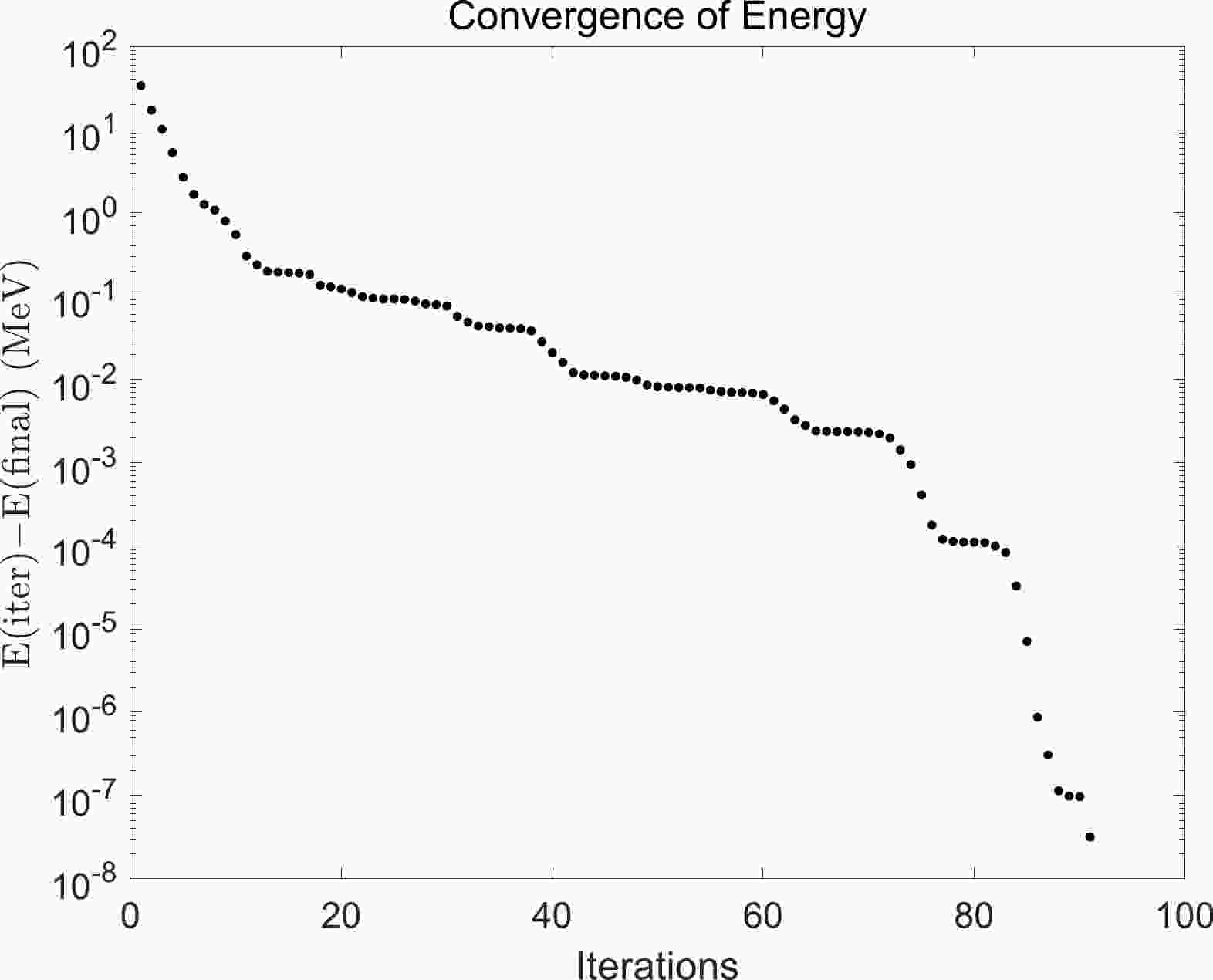
$ \overline{E} $ converges in Step 2 as the number of iteration increases. The dimension of the model in this case was$ D = 2\Omega = 40 $ (20 above the Fermi surface and 20 below the Fermi surface), as previously explained. The energy error decreases on the semi-log plot. After approximately 90 iterations, the error was less than$ 10^{-7} $ MeV. The total time cost of all iterations was 2.118 s using double precision.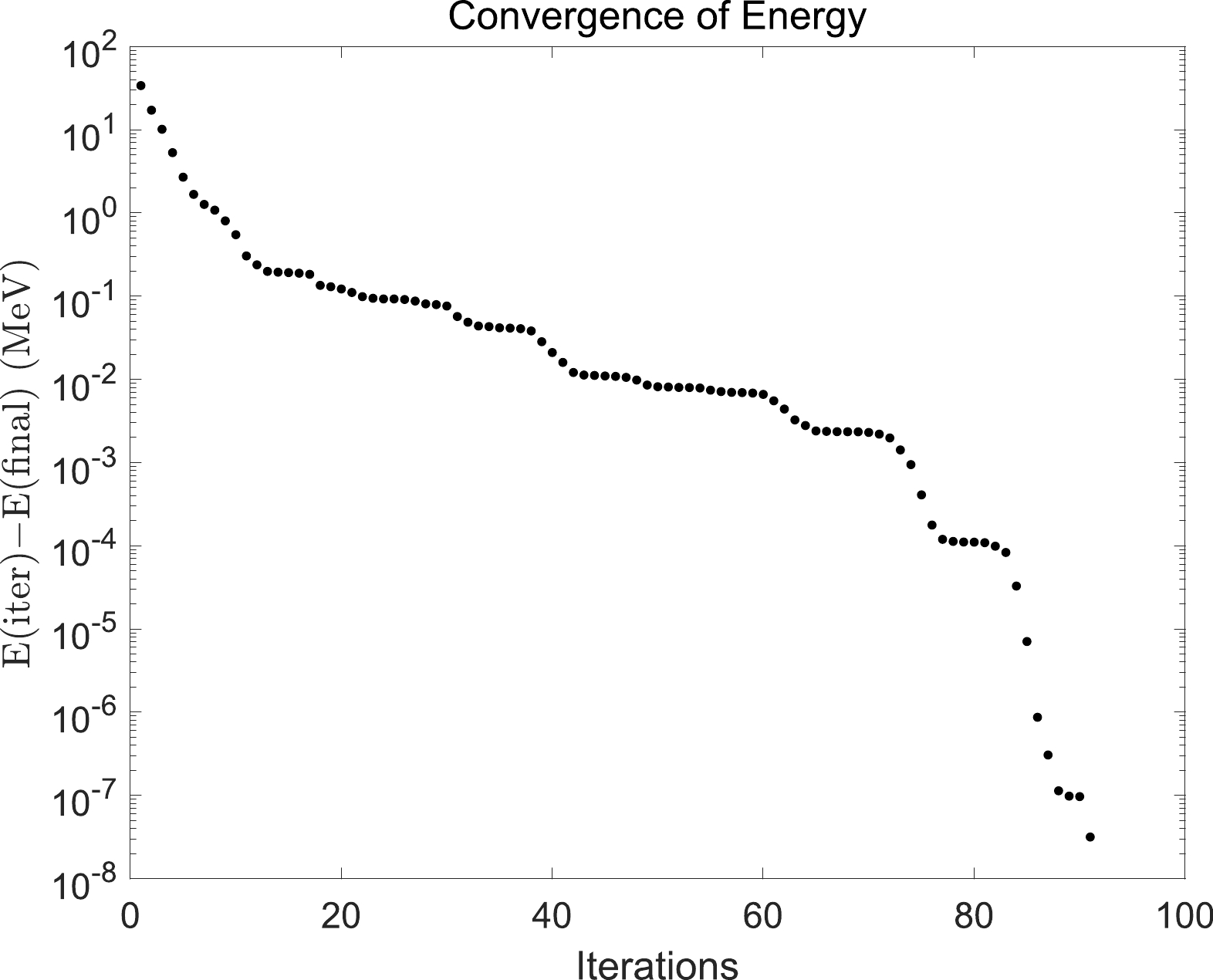
Figure 1. Convergence of energy in Step 2 using double precision. The horizontal axis represents the number of iterations. The vertical axis shows the energy at each iteration E(iter), relative to the final converged energy E(final). The total time cost of all iterations was 2.118 s using a laptop (Intel Core i7-8550U @ 1.80 GHz, 32.0 GB RAM, no parallel computing).
Figure 2 shows how
$ \overline{E} $ converges in Step 3. The lowest 240 single-particle orbits (94 below the Fermi surface and$ 240 - 94 = 146 $ above the Fermi surface) were selected, considering that the level density in the upper layer is relatively small. Therefore, the number of single-particle orbits above the Fermi surface was slightly larger. Its dimension$ D = 2\Omega=240 $ was the largest dimension set in this study because of the limited computing resources available. The computer code was run twice using double precision and 120 precision, respectively. The legend "120 digits" denotes the use of 120 precision everywhere, whereas the legend "double" denotes the use of 120 effective digits only when necessary (to overcome the sign problem), switching to double precision for higher speed. Comparing these two executions, "120 digits" was significantly slower than "double", but it converged to higher precision.
Figure 2. (color online) Energy and time using two types of precision: double and 120 effective digits. The solid and dashed lines correspond to the left vertical axis and show the energy at each iteration E(iter), relative to the final converged energy E(final). The dotted and dash-dot lines correspond to the right vertical axis, showing the accumulated computer time cost after each iteration.
In practical terms, the energy
$ \overline{E} $ can be minimized to any arbitrary precision. The energy error decreased linearly on the semi-log plot for the "120 digits" execution, as shown in Fig. 2, so$ \overline{E} $ converged exponentially with the number of iterations. After 120 iterations, the error was less than$ 10^{-50} $ MeV. It is not difficult to conclude that if the precision used in Step 3 (greater than 120) is increased and more iterations are carried out, the precision of the convergent energy will increase as well. For the "double" execution, the best precision achievable was approximately$ 10^{-23} $ MeV, reached near the 55th iteration. This execution produced the same result as that of the "120 digits" execution until this point (the two energy curves are indistinguishable). After this point, the precision of the "double" execution fluctuated and no improvement was achieved. To summarize, the "double" execution is preferred because it runs much faster and the precision of$ 10^{-23} $ MeV is sufficient in nuclear physics.The cost of computing time per iteration is primarily determined by the dimension of the single-particle model space. For the "double" run,
$ T \approx (D/82.5)^{3.38} $ , as shown in Fig. 3, where T is the average time of one iteration (averaged over 20 iterations) in unit of second and$ D = 2\Omega $ is the dimension. For the "120 digits" run,$ T \approx (D/61.0)^{4.11} $ . All the numerical computations were completed on a laptop having a one quad-core CPU (Intel Core i7-8550U @ 1.80 GHz), dual 16.0 GB memory (32.0 GB in total, operating at 2400 MHz). A single core was employed in all computations (i.e., no parallel computing was set). All the time costs given in the text or plotted in the figures represent actual time costs on this laptop.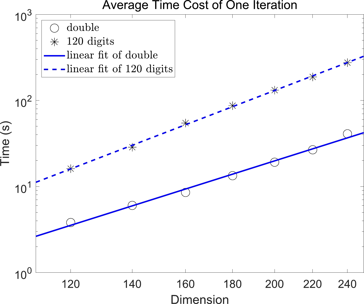
Figure 3. (color online) Average computing time cost of one iteration in different model spaces. The horizontal axis represents the dimension of each model space, whereas the vertical axis represents the time cost of one iteration (averaged over 20 iterations). The circle symbols represent iterations using double precision, while the asterisk symbols represent iterations using 120 effective digits. The solid and dashed lines represent their linear fits, respectively.
A complete execution is shown in Fig. 4. The exact energy E(exact) is the energy after 120 iterations using random three-body forces with 120 precision when the dimension is equal to 240 (the maximum dimension, maximum precision, and maximum number of iterations employed in a single program execution in this study). This energy is the smallest energy considered in this work; it is more precise than
$ 10^{-50} $ MeV (see Fig. 2) and is regarded as the physically real energy of this system. Step 1 was HF and incurred negligible time. The energy error after step 2 was approximately 8 MeV, which means that the VS1 energy minimum was higher than the VS2 energy minimum by approximately 8 MeV (the dimension of VS1 was$ D=40 $ whereas that of VS2 was$ D=240 $ ), because the randomly generated$ G_{\alpha\beta,\gamma} $ and$ F_{\alpha\beta\gamma} $ did not decrease as$ | e_{\gamma} - e_{\alpha} | $ (or$ | e_{\gamma} - e_{\beta} | $ ) increased. After the three steps, the energy error was reduced to approximately 2 keV in less than 7 min. Figure 5 plots the energy convergence pattern in different model spaces. The energy error curves are linear on a semi-log plot, so the energy converges exponentially with increasing number of iterations. As the dimension of model space increased, the rate of convergence did not slow down significantly. For a specified dimension, the cumulative time cost increased linearly with the number of iterations. Therefore, the time cost was approximately the same for each iteration. Note also that increasing the dimension of the model space by 40 approximately doubles the time cost of a single iteration.
Figure 4. Energy and time in a complete run. The horizontal axis represents the three steps listed in Sec. V, where Step 3 is divided into 10 iterations. The cross symbols correspond to the left axis and show the energy error after each step or iteration, relative to the exact energy E(exact) (converged energy in
$ D=240 $ model space). The circle symbols correspond to the right axis and show the time cost spent by each step or iteration, in unit of second.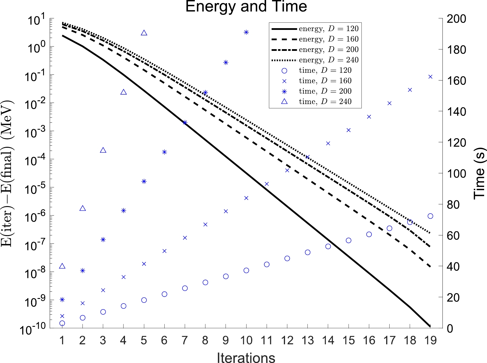
Figure 5. (color online) Energy and time in different model spaces. The solid, dashed, dash-dot, and dotted lines correspond to the left vertical axis, and show the energy errors. The circle, cross, asterisk, and triangle symbols correspond to the right vertical axis, and show the accumulated time cost after each iteration.
The asymptotic expressions (37a) and (37b) faithfully reproduce the exact values of
$ v_{\alpha} $ (35a) and (35b) away from the Fermi surface. Figure 6 compares them at the energy minimum in the$ D=240 $ model space. Near the Fermi surface (i.e., the vicinity of$ v_{\alpha} = 1 $ ), the asymptotic expressions (37a) and (37b) are not applicable, so the largest absolute value of relative error$ |RE| \approx 1 $ appears here. Going away from the Fermi surface,$ |RE| $ becomes gradually smaller. Of these 120 different values of$ v_{\alpha} $ , 82.5% have$ |RE| < $ 10% and 36.7% have$ |RE| < $ 1%. Figure 7 shows that the average computing time cost per one iteration of both exact$ v_{\alpha} $ and asymptotic$ v_{\alpha} $ increases approximately linearly with the dimension on the log-log plot. For the exact$ v_{\alpha} $ run, the circle symbols and solid line are exactly the same as the ones for the "double" run displayed in Fig. 3, so$ T \approx (D/82.5)^{3.38} $ . For the asymptotic$ v_{\alpha} $ run,$ T \approx (D/198)^{2.12} $ ; it was a much faster execution.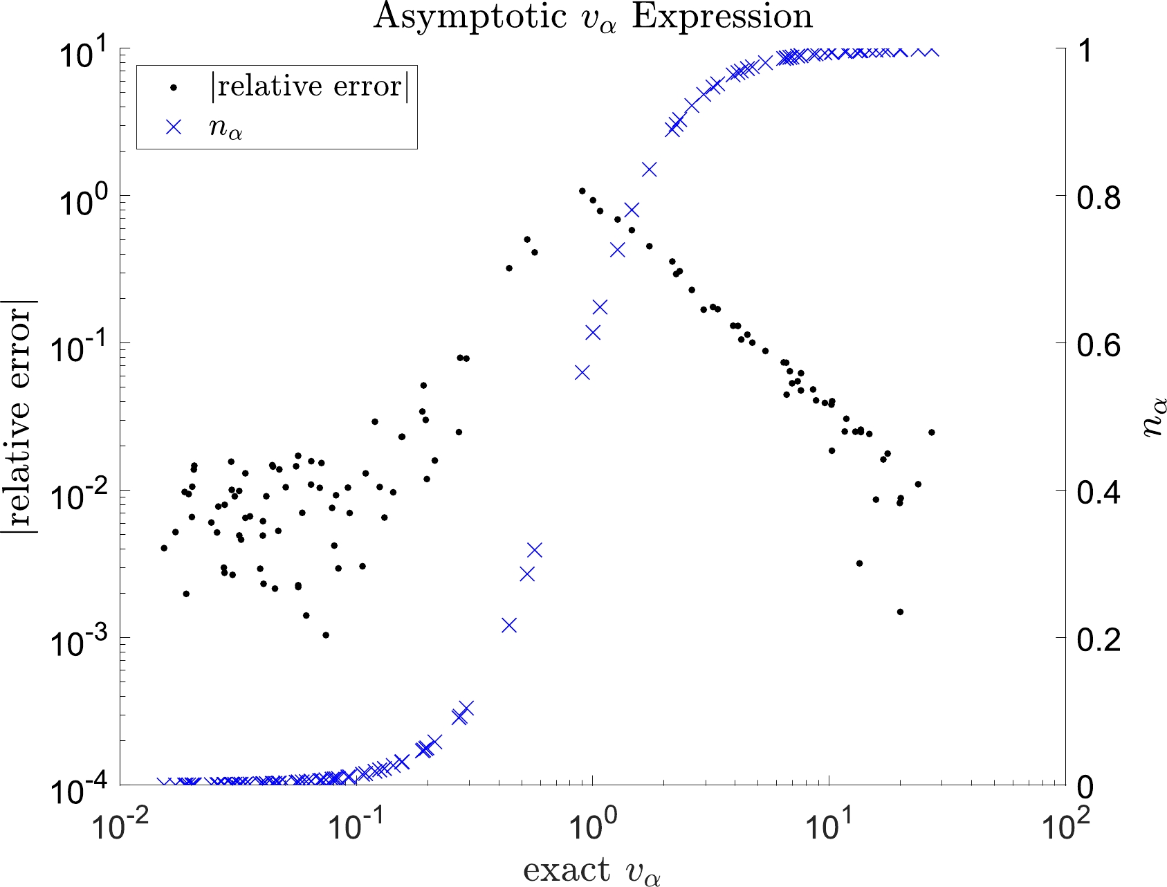
Figure 6. (color online) Error of the asymptotic
$ v_{\alpha} $ as a function of the exact value of$ v_{\alpha} $ . The relative error is given by$RE \equiv (v_{\alpha}^{\rm asymptotic}/v_{\alpha}^{\rm exact}) - 1$ . The horizontal axis represents the exact$ v_{\alpha} $ . The dot symbols correspond to the left vertical axis and show$ |RE| $ . The cross symbols correspond to the right vertical axis and represent the exact occupation number$ n_{\alpha} $ .
Figure 7. (color online) Average computing time cost of one iteration in different model spaces. The horizontal axis represents the dimension of each model space, whereas the vertical axis represents the time cost of one iteration (averaged over 20 iterations). The circle symbols represent iterations according to the exact
$ v_{\alpha} $ expressions (35a) and (35b), while the triangle symbols represent iterations according to the asymptotic$ v_{\alpha} $ expressions (37a) and (37b). The solid and dash-dot lines represent their linear fit, respectively.Figure 8 illustrates a portion of the convergence criteria in this program, using 120 precision and
$ D=240 $ model space. After convergence, all five criteria in the figure should be equal to zero. Here "equal to zero" means a non-specific, acceptable error. It can be seen that all five criteria decreased linearly in the semi-log plot as the number of iterations increased. After 20 iterations, all the convergence criteria were reduced by at least four orders of magnitude. There are three additional criteria not shown in the figure;${\rm max}[(\partial \overline{E}/\partial v_{\alpha})_{(a)}-(\partial \overline{E}/\partial v_{\alpha})_{(b)}]$ ,$ \sum\limits_{\alpha\in\Theta} v_{\alpha} (\partial \overline{E}/\partial v_{\alpha})_{(a)} $ , and$ \sum\limits_{\alpha\in\Theta} v_{\alpha} (\partial \overline{E}/\partial v_{\alpha})_{(b)} $ are always zero during 200 iterations, which further proves that the energy truly converges.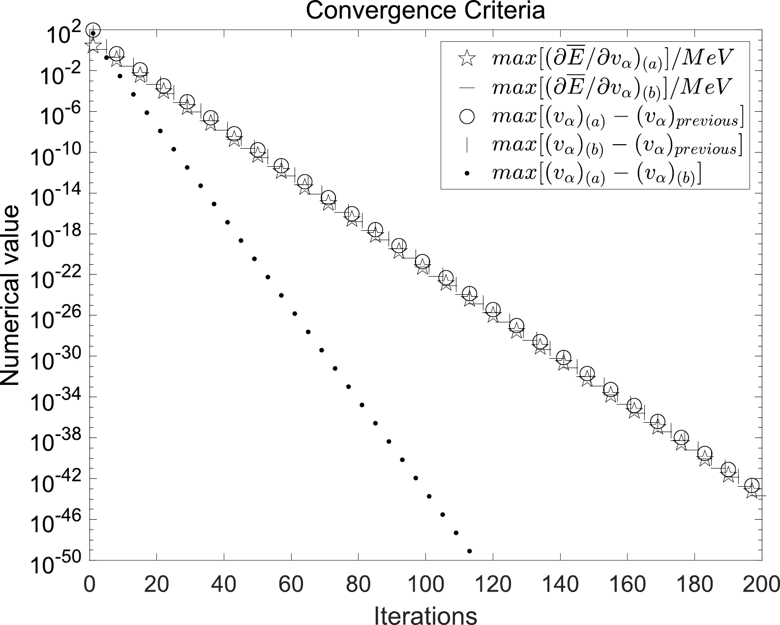
Figure 8. Partial convergence criteria in one program execution. The horizontal axis represents the number of iterations whereas the vertical axis represents the numerical value of each expression. The pentagram and horizontal line symbols represent the maximum numerical values of (32a) and (32b), respectively. The circle (vertical line) symbols represent the maximum numerical value of the difference between (35a) and (35b) in the current iteration and exact
$ v_{\alpha} $ in the previous iteration. The point symbols represent the maximum numerical value of the difference between (35a) and (35b).We ran the extended VDPC+BCS code six times, each running through the first and second steps. The second step was iterated 51 times. These six times used different three-body strength and/or degree of dispersion, as shown in Fig. 9. The dash-dotted line
$ coef =0 $ corresponds to no three-body interaction, only one-body, and two-body interactions. The values represented by the circle symbol are used in all previous figures and are also described in the first paragraph of this section. It can be seen from the figure that after the three-body force is added, the energy converges faster, and when other conditions remain unchanged, the greater the three-body strength, the faster the energy convergence, and the positive or negative nature of the three-body force will not affect the convergence speed. By comparing the solid line and circle symbol, we can conclude that the degree of dispersion does not affect the convergence speed. The triangle symbol means that after a more realistic simulation of the three-body force (the three-body force matrix elements rapidly become smaller as α, β, and γ get away from each other), the energy convergence curve will be closer to the curve of only one-body and two-body interactions, but it will converge faster, and the accuracy will be higher after the same number of iterations. By using different random three-body force matrices$ G_{\alpha\beta,\gamma} $ and$ F_{\alpha\beta\gamma} $ , it is shown that the three-body force is correctly added in this study, regardless of the three-body force used, and including the real three-body force. Indeed, it can be correct and quickly converge to any arbitrary precision.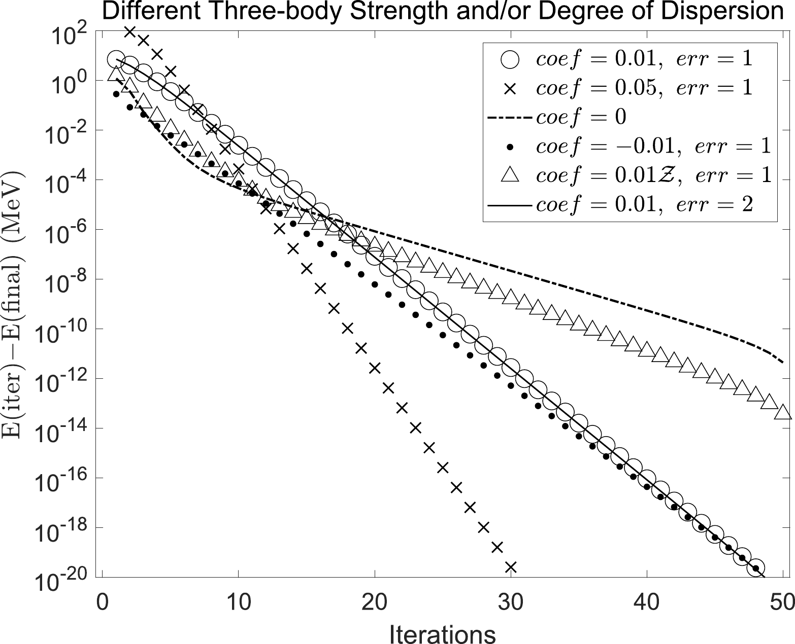
Figure 9. Convergence of energy using different three-body Hamiltonians in the
$ D=240 $ model space. The six curves correspond to six executions using different three-body strength$ coef $ and/or degree of dispersion$ err $ . For each execution, its curve shows the energy at every iteration E(iter), relative to the final converged energy E(final) in this execution.$ \mathit{Z} $ is a coefficient whose value ranges between 0.1 and 1 and decreases sharply as γ moves away from α and β. -
This study extends the VDPC+BCS formalism by including three-body forces. In particular, the average energy and its gradient are derived for a three-body Hamiltonian in terms of the coherent-pair structure
$ v_{\alpha} $ . The gradient is vanished to obtain the analytical expression of$ v_{\alpha} $ at the energy minimum. The extended VDPC+BCS algorithm iterates on these$ v_{\alpha} $ expressions to minimize the average energy for a three-body Hamiltonian, until arbitrary precision. Asymptotic expressions of$ v_{\alpha} $ away from (above or below) the Fermi surface are also provided. They are highly accurate, as shown in Fig. 6, and can be numerically evaluated quickly, as shown inFig. 7.The new code is demonstrated using a numerical example with realistic two-body and random three-body forces in large model spaces. Figure 4 shows a complete numerical example execution. In the given model space, the average energy
$ \overline{E} $ can be minimized to any arbitrary precision, as shown in Fig. 2. The pattern of energy convergence and real computer time cost are presented in Fig. 5. The numerical sign problem emerges in some areas of the code if double-precision floating-point numbers are used globally. In these parts, higher precision (120 effective digits) was employed to solve this issue. Numerical expressions of the computing time cost per iteration are also provided using the dimension of the single-particle model space, as shown in Fig. 3. The new code is published together with this manuscript.In the future, realistic three-body forces will be employed to study their effect on the coherent-pair condensate. Possible changes of various pairing phenomena will also be studied.
-
The author gratefully acknowledges discussions with Prof. L. Y. Jia.
Extending the VDPC+BCS formalism by including three-body forces
- Received Date: 2022-06-15
- Available Online: 2023-04-15
Abstract: Recently, Jia proposed a formalism to apply the variational principle to a coherent-pair condensate for a two-body Hamiltonian. The present study extends this formalism by including three-body forces. The result is the same as the so-called variation after particle-number projection in the BCS case, but now, the particle number is always conserved, and the time-consuming projection is avoided. Specifically, analytical formulas of the average energy are derived along with its gradient for a three-body Hamiltonian in terms of the coherent-pair structure. Gradient vanishment is required to obtain analytical expressions for the pair structure at the energy minimum. The new algorithm iterates on these pair-structure expressions to minimize energy for a three-body Hamiltonian. The new code is numerically demonstrated when applied to realistic two-body forces and random three-body forces in large model spaces. The average energy can be minimized to practically any arbitrary precision.


 DownLoad: