


 Abstract
 HTML
HTML Reference
 Related
 PDF
PDF


-
Typically, energy losses resulting from neutrino emissions are important in astrophysical problems. Neutrinos are produced in stellar interiors; owing to their weak interactions with stellar matter, they can easily absorb energy that would otherwise take much longer to be transported to the surface via radiation or convection. The resulting energy accumulating at the center of the star dictates its rate of nuclear burning, structure, and evolution, and ultimately the death cycle. In this case, the production of neutrino pairs represents an extremely important energy-loss mechanism for stars with certain densities and temperatures. The photoneutrino process was first studied by Ritus [1] and Chiu and Stabler [2] for non-degenerate and degenerate electrons in the Fermi
$ V-A $ theory. Beaudet, Betrosian, and Salpeter [3] provided analytical approximations for the photo-neutrino process within the same model. Dicus [4] reanalyzed this process within the framework of the standard model (SM). The author introduced certain global correction factors into these rates to incorporate neutral current effects. Schinder et al. [5] numerically recalculated the emission rates within the SM and noted good agreement with the BPS formulas in the temperature range of$10^{10} -10^{11}\rm K$ . In 1989, Itoh et al. [6] improved their previous study [7] and provided an alternate set of approximation formulas. In all of these previous studies, photons were assumed to be ordinary photons. Typically, for an ordinary photon, this process is expected to play an important role for low density matter with$\rho/\mu_e = 10^5\rm~ gr/cm^3$ and a comparatively low temperature$T = 4\times 10^8~\rm K$ . The foregoing calculations have been performed approximately sixty years ago by several authors investigating the$ V-A $ model [1–3], SM [4–12], and magnetic model [13]. Instead of considering ordinary photons, Dutta et al. [10,11] considered a massive photon (plasmon) and the angular dependence of the emitted neutrinos in a process involving hot and dense matter. In a previous study, the authors did not consider the energy and angular dependencies of the neutrinos in the calculations of the total energy loss rates because they used Lenard's formula [14]. They presented numerical results under widely varying conditions of the temperature and density.In recent studies, we investigated the production of neutrino pairs, their energy losses [15], and energy deposition rates [16] in the minimal extension of the SM. Notably, the photo-neutrino, plasmon and bremstrahlung processes are the dominant causes of stellar energy losses in different regions within the density-temperature plane. The calculations involved in this study could contribute to a better understanding of neutrino physics and new physics beyond the SM.
In this study, we investigated the energy loss rates associated with the photo-neutrino pair annihilation process
$ e^- + \gamma \rightarrow e^- + \nu_e +\overline{\nu}_e $ considering the effect of neutrino electromagnetic form factors (such as charge radius and anapole moment) on neutrino-photon interactions in the extended SM. This was accomplished by considering the$ \gamma \nu \overline{\nu} $ vertex for Dirac neutrinos [15–31], as detailed in Sec. II. Note that previous studies have not considered these effects. In Sec. III, we present the obtained numerical results, followed by a discussion and conclusion. -
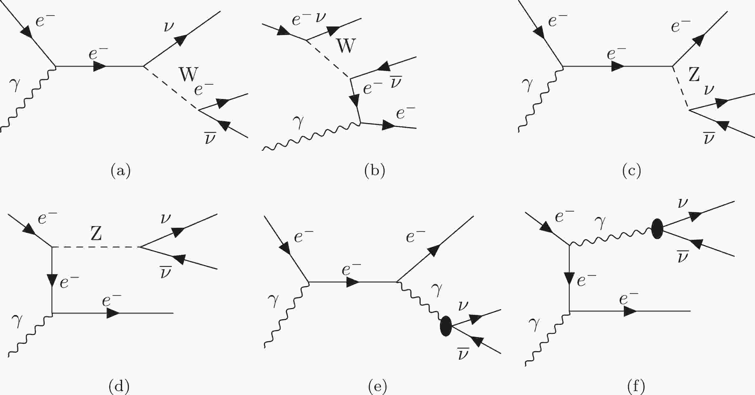
Feynman diagrams for the following process
$ e^-(p) + \gamma (k) \rightarrow e^-(p') + \nu_e(q_1) +\overline{\nu}_e(q_2) $ are presented in Fig. 1. Symbols in parentheses denote particles momenta.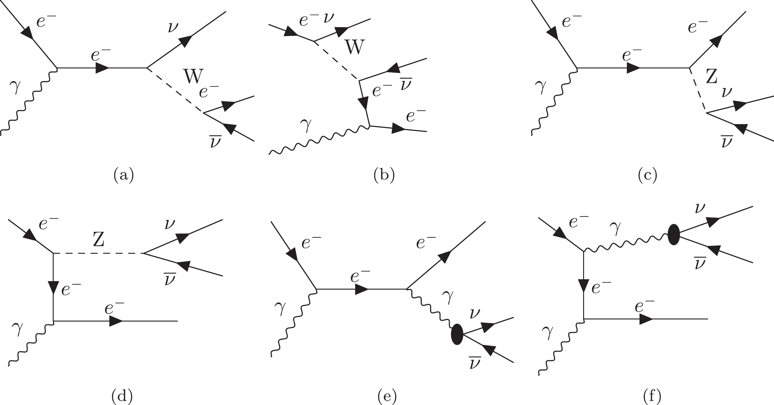
Figure 1. Leading order Feynman diagrams for the photo-neutrino process. The black disks in (e) and (f) represent the effective neutrino interactions beyond the SM.
After a Fierz transformation, the matrix element of the process within the SM framework (Figs. 1(a)–(d)) with a low energy limit can be written as
$ \begin{aligned}[b] \\[-6pt] \mathcal{M}^{\rm(SM)} = & - {{\rm i}e G_{\rm F} \over \sqrt{2}} \Bigg[ \overline{ \mathfrak{u}}_e(p') \gamma^\beta (C_V-C_A \gamma_5) \frac{( {\not p}+ {\not k}+m_e)}{2pk+k^2} {\not \epsilon} \mathfrak{u}_e(p) + \overline{ \mathfrak{u}}_e (p') {\not \epsilon} \frac{( {\not p}'- \not{k}+m_e)}{-2p'k+k^2} \gamma_\beta (C_V-C_A \gamma_5) \mathfrak{u}_e(p) \Bigg] \\ & \times \overline{ \mathfrak{u}}_\nu(q_1) \gamma_\beta (1- \gamma_5) {v}_{\overline{\nu}}(q_2), \end{aligned} $ 
(1) where
$ \mathfrak{u} $ and$ {v} $ denote Dirac spinors,$ C_V={\dfrac{1}{ 2}} +2 \sin^2 \theta_W $ and$ C_A={\dfrac{1}{ 2}} $ for$ \nu_e $ , and$ C_V=-{\dfrac{1}{ 2}} +2 \sin^2 \theta_W $ and$ C_A=-{\dfrac{1}{ 2}} $ for$ \nu_\mu $ and$ \nu_\tau $ because electron neutrinos interact with both W and Z bosons; however, muon and tau neutrinos interact only with Z bosons (see the case in Figs. 1(c) and (d)). In this study, we restrict our calculations by considering only electron neutrinos.The matrix element presented in Figs. 1 (e) and (f) is given by
$ \begin{array}{*{20}{l}} \mathcal{M}^{(\gamma)}= \mathcal{M}^{(Q)} + \mathcal{M}^{(\mu)} ,\end{array} $

(2) where
$ \begin{aligned}[b] \\[-5pt] \mathcal{M}^{(Q)} = & {{\rm i} 4\pi\alpha \over q^2} \overline{ \mathfrak{u}_\nu}(q_1) \left(\gamma^\beta - {q^\beta { {\not q}} \over q^2}\right) \left[ {q^2 \over 6} <r_\nu^2> \right] {v}_{\overline{\nu}}(q_2) \\ & \times ({\rm i}e)^2 \left[ \overline{ \mathfrak{u}}_e(p') \gamma^\beta \frac{( {\not p}+ {\not k}+m_e)}{2pk+k^2} {\not \epsilon} \mathfrak{u}_e(p) + \overline{ \mathfrak{u}}_e (p') {\not \epsilon} \frac{( {\not p}'- {\not k}+m_e)}{-2p'k+k^2} \gamma_\beta \mathfrak{u}_e(p) \right], \end{aligned} $ 
(3) $ \begin{aligned}[b] \mathcal{M}^{(\mu)} = & -{\rm i} {2\pi\alpha \over q^2} \overline{ \mathfrak{u}_\nu}(q_1) \sigma^{\beta \lambda} q_\lambda \left[ \mu \right] {v}_{\overline{\nu}}(q_2) \\ & \times ({\rm i} e)^2 \left[ \overline{ \mathfrak{u}}_e(p') \gamma^\beta \frac{( {\not p}+ {\not k}+m_e)}{2pk+k^2} \not {\epsilon} \mathfrak{u}_e(p) + \overline{ \mathfrak{u}}_e (p') {\not \epsilon} \frac{({ \not p}'- {\not k}+m_e)}{-2p'k+k^2} \gamma_\beta \mathfrak{u}_e(p) \right], \end{aligned} $

(4) where
$ q = q_1 + q_2 $ ,$ \alpha=e^2/4\pi $ is the fine structure constant,$ <r_\nu^2>=<r^2>+6 \gamma_5 a $ is the mean charge radius of a neutrino (in fact, it is the squared charge radius), and$\mu= \mu_\nu+ {\rm i} \gamma_5 d_\nu$ is the neutrino magnetic moment [15, 23].The total matrix element for the process can be written as
$ \begin{array}{*{20}{l}} \mathcal{M}_t = \mathcal{M}^{\rm (SM)}+ \mathcal{M}^{(Q)} + \mathcal{M}^{(\mu)} . \end{array} $

(5) Notably, no interference occurs between the helicity-conserving (
$\mathcal{M}^{\rm(SM)}$ and$ \mathcal{M}^{(Q)} $ ) and helicity-flipping ($ \mathcal{M}^{(\mu)} $ ) amplitudes. Thus, combining the helicity-conserving amplitudes and using$ q_\mu J^\mu(q)=0 $ , we determine the following:$ \begin{aligned}[b] \mathcal{M}^{\rm (SM)} + \mathcal{M}^{(Q)} = & {{\rm i} e G_{\rm F} \over \sqrt{2}} \Bigg[ \overline{ \mathfrak{u}}_e(p') \gamma^\beta (C'_V - C_A \gamma_5) \frac{( {\not p} + {\not k} + m_e)}{2pk+k^2} {\not \epsilon} \mathfrak{u}_e(p)\\& + \overline{ \mathfrak{u}}_e (p') {\not \epsilon} \frac{( {\not p}'- {\not k}+m_e)}{-2p'k+k^2} \gamma_\beta (C'_V-C_A \gamma_5) \mathfrak{u}_e(p) \Bigg] \\ & \times \overline{ \mathfrak{u}}_\nu(q_1) \gamma_\beta (1- \gamma_5) {v}_{\overline{\nu}}(q_2), \end{aligned} $

(6) where
$C'_V = C_V + \dfrac{\sqrt{2} \pi \alpha}{ 3 G_{\rm F}} < r_\nu^2 >$ [15, 16, 18–21, 28, 30, 31]. We neglect the helicity-flipping amplitudes because the contribution of the magnetic moment term ($ \mathcal{M}^{(\mu)} $ ) is negligible for$\mu_{\nu_e} \le 10^{-12} \mu_{\rm B}$ [32–35] and$\mu_{\nu_\tau} \le 10^{-10} \mu_{\rm B}$ [36].Thus, the total matrix element square can be written as
$ \begin{array}{*{20}{l}} | \mathcal{M}_t|^2 = | \mathcal{M}^{\rm(SM)} + \mathcal{M}^{(Q)}|^2 . \end{array} $

(7) The total energy loss rate (
$ \mathcal{Q} $ ) or emissivity energy carried away by the neutrino pair per unit volume per unit time owing to the photo-neutrino process is given by [3, 4]$ \begin{aligned}[b] \mathcal{Q} = & {1 \over (2\pi)^{11}} \int {{\rm d}^3 p \over 2E} \left[{ 2 \over {\rm exp}[(E-\mu_e)/k_{\rm B} T]+1} \right] \\&\times\int {{\rm d}^3 k \over 2\omega}{2 \over {\rm exp}[\omega/k_{\rm B} T]-1}\\&\times \int {{\rm d}^3 p' \over 2E'} \left[ 1- { 1 \over {\rm exp}[(E'-\mu_e)/k_{\rm B} T]+1} \right] \\ \\ & \times (E + \omega - E') \int {{\rm d}^3 q_1 \over 2E_\nu} \int {{\rm d}^3 q_2 \over 2E_{\overline{\nu}}} (2\pi)^4 \\&\times \delta^4 (p+k-p'-q_1-q_2) {1 \over 4} \sum\limits_{s,\epsilon} | \mathcal{M}_t|^2 , \end{aligned} $

(8) where
$ p=(E,\overrightarrow{p}) $ ,$ p'=(E',\overrightarrow{p'}) $ ,$ k=(\omega,\overrightarrow{k}) $ ,$ q_1=(E_\nu,\overrightarrow{q}) $ , and$ q_2=(E_{\overline{\nu}},\overrightarrow{q'}) $ denote the five momenta of the incoming and outgoing electrons, photon, neutrino, and anti-neutrino, respectively.$ \mu_e $ is the electron chemical potential,$k_{\rm B}$ is the Boltzmann constant, and T is the stellar temperature. The factor$ 2 $ in front of the electron distribution function$f_e(E) = [{\rm exp}[(E-\mu_e)/ k_{\rm B} T]+ 1]^{-1}$ and photon distribution function$f_\gamma(\omega) = \big({\rm exp}[\omega/ k_{\rm B} T]- 1\big)^{-1}$ accounts for the two spin states of the corresponding particles, whereas the factor$ \dfrac{1}{4} $ corresponds to the average over initial spin states. In the sum of Eq. (8), the index s indicates sums over the electron spin states, whereas$ \epsilon $ indicates a sum over the photon polarization. The factor$\left[1- \Big({\rm exp}[(E'- \mu_e)/ k_{\rm B} T]+ 1 \right)^{-1} \Big]$ accounts for the Pauli-blocking factor of outgoing electrons. Note that the energy loss rate$ \mathcal{Q} $ in Eq. (8) cannot be calculated analytically for all temperatures and chemical potentials.The sum of photon polarization is performed in terms of its longitudinal and transverse components
$ \sum\limits_{\lambda=1}^2 \epsilon^{\mu\star} \epsilon^\nu = - g^{\mu\nu} + {k^\mu k^\nu \over k^2} = P_ \mathcal{L}^{\mu\nu} + P_ \mathcal{T}^{\mu\nu} ,$

(9) where the longitudinal and transverse components are given as
$ P_ \mathcal{L}^{\mu\nu} = \sum\limits_{\lambda=1}^2 \epsilon^{\star\mu} \epsilon^\nu - P_ \mathcal{T}^{\mu\nu}, $

(10) $ \begin{array}{*{20}{l}} P_ \mathcal{T}^{\mu\nu} = \left\{ \begin{array}{lcr} \delta^{ij} - \dfrac{k^i k^j }{ k^2}, & \rm{ for } & i,j=1,2,3 \\ \\ 0, & \rm{ for } & \mu ~ \rm{ or }~ \nu = 0 . \end{array} \right. \end{array} $

(11) The photon polarization tensor mentioned above performs the following functions
$ \begin{aligned}[b]& P_ \mathcal{T}^{\mu\beta} P_{ \mathcal{L} \beta \nu} = 0 \, , \quad P_ \mathcal{L}^{\mu\beta} P_{ \mathcal{L} \beta \nu} = - P_{ \mathcal{L}\nu}^\mu \, ,\quad \\& P_ \mathcal{T}^{\mu\beta} P_{ \mathcal{T} \beta \nu} = - P_{ \mathcal{T} \nu}^\mu \, ,\quad P_{ \mathcal{L}\mu}^\mu = -1 \, ,\quad P_{ \mathcal{T}\mu}^\mu = -2 . \end{aligned} $

Using these relations, one can express the longitudinal (
$ \mathcal{L} $ ) and transverse ($ \mathcal{T} $ ) components of the squared total matrix elements as follows.$ \begin{aligned}[b] \sum\limits_{s,\epsilon} | \mathcal{M}_t^{( \mathcal{L}, \mathcal{T})}|^2 =& 32 e^2 G_{\rm F}^2 \Big\{ (C_V^{\prime 2}-C_A^2) m_e^2 | \mathcal{M}_-^{( \mathcal{L}, \mathcal{T})}|^2 \\&+ (C_V^{\prime 2}+C_A^2) | \mathcal{M}_+^{( \mathcal{L}, \mathcal{T})}|^2 + C_V^{\prime}C_A | \mathcal{M}_{+-}^{( \mathcal{L}, \mathcal{T})}|^2 \Big\}. \end{aligned} $

(12) In Eq. (12), we do not present the expressions for
$| \mathcal{M}_-^{(\mathcal{L}, \mathcal{T})}|^2 $ ,$ | \mathcal{M}_+^{(\mathcal{L}, \mathcal{T})}|^2$ , and$ | \mathcal{M}_{+-}^{(\mathcal{L}, \mathcal{T})}|^2 $ because they are lengthy. Our calculations are parallel with those performed by Dutti et al. (see [11] for the details).Integrating the momentum p and k, we obtain
$ \begin{aligned}[b] I(p',q_1,q_2) =& {1 \over \pi^2} \int {{\rm d}^3 p \over 2E} \int {{\rm d}^3 k \over 2\omega} f_\gamma(\omega) f_e(E)\\&\times \delta^4(p+k-p'-q_1-q_2) \sum\limits_{s,\epsilon} | \mathcal{M}_t^{( \mathcal{L}, \mathcal{T})}|^2 . \end{aligned} $

(13) Following this, for the total energy loss, we have
$ \begin{aligned}[b] \mathcal{Q} =& {1 \over (2\pi)^9} \int {{\rm d}^3 q_1 \over 2E_\nu} \int {{\rm d}^3 q_2 \over 2E_{\overline{\nu}}} \int {{\rm d}^3 p' \over 2E'}\\&\times \left[ 1 - f_e(E') \right] (E+\omega-E') I(p',q_1,q_2) . \end{aligned} $

(14) If we denote the angle between
$ \overrightarrow{p}+\overrightarrow{k} $ and$ \overrightarrow{k} $ as$ \theta_k $ , we obtain$ \begin{aligned}[b] I(p',q_1,q_2) =& {1 \over 4 (2\pi)^2} \int_0^\infty {|\overrightarrow{k}| \over \omega} {\rm d}|\overrightarrow{k}|\\&\times \int_0^{2\pi} {\rm d} \varphi_k f_\gamma(\omega) f_e(E) {1 \over |\overrightarrow{p}+\overrightarrow{k}| } \sum\limits_{s,\epsilon} | \mathcal{M}_t^{( \mathcal{L}, \mathcal{T})}|^2 . \end{aligned} $

(15) Finally, for the differential energy loss from Eq. (14), we obtain the following:
$ \begin{aligned}[b] {{\rm d}^3 \mathcal{Q} \over {\rm d} E_\nu {\rm d} E_{\overline{\nu}}{\rm d} (\cos \theta_{\nu\overline{\nu}})} =& {\pi^2 \over (2\pi)^9} E_\nu E_{\overline{\nu}} \int_0^\infty {|\overrightarrow{p'}|^2 \over E'} {\rm d} |\overrightarrow{p'}| \int_{-1}^1 {\rm d} (\cos \theta_e) \\&\times\int_0^{2\pi} {\rm d} \phi_e \,\, [1-f_e(E')](E_\nu + E_{\overline{\nu}}) \\&\times I(p',q_1,q_2) . \end{aligned} $

(16) In the leading order, the dispersion relations of photons in plasma for the photo-neutrino process are
$ \omega_L^2 = \omega_P^2 \, , \quad \omega_T^2 = \omega_P^2 + |\overrightarrow{k}|^2 , $

where
$ \omega_P $ is the plasma frequency.To gain better insights into the relationship between temperature and neutrino emissivity, it is helpful to identify the most critical physical scales involved in the photo-neutrino production process of neutrino pairs in limited situations. This can provide a qualitative and, in some cases, quantitative comprehension. We can obtain degenerate plasmas that occur at all temperatures at sufficiently high densities and non-degenerate relativistic plasmas that occur at high temperatures and low densities.
We investigate the term
$ \mathcal{Q}_ \mathcal{T} $ for the transverse case, and the analysis for the longitudinal case can be performed in a similar manner. Although we cannot calculate the total energy loss rate analytically for all T and$ \mu_e $ , we consider evaluating ($ \mathcal{Q} $ ) in three different regions, where it can be analyzed analytically for nondegenerate, intermediate, and degenerate electrons. -
This case occurs at low enough densities, for which
$ \mu_e - m_e \ll T $ . For$T \ge 10^{10}~\rm K$ , the electron mass can be neglected in comparison to$ \mu_e $ . In the relativistic case, the electron density and plasma frequency are expressed as [37]$ n_e = {\mu_e \over 3 \pi^2}(\mu_e^2 + T^2 \pi^2) \simeq {\mu_e T^2 \over 3}, $

$ \omega_p^2 = {4 \alpha \over 3 \pi }\left(\mu_e^2 + {T^2 \pi^2 \over 3}\right) \simeq 4 \pi \alpha {T^2 \over 9} \, . $

In this case, both the electron momentum and energy are of the order of
$ E \simeq |\overrightarrow{p}| \simeq T $ , and similarly, both the photon momentum and energy are$ \omega \simeq |\overrightarrow{k}| \simeq T $ . Therefore, we obtain the squared total matrix element as$ \sum\limits_{s,\epsilon} | \mathcal{M}_t^ \mathcal{T}|^2 \simeq 256 \pi \alpha G_{\rm F}^2 (C_V^{'2} + C_A^2) E E_\nu E_{\overline{\nu}} / E' . $

(17) Subsequently, performing phase space integration results in the following:
$ \begin{aligned}[b] \mathcal{Q}_ \mathcal{T} =& {20 \alpha G_{\rm F}^2 (C_V^{'2} + C_A^2) \over 3 (2\pi)^6} T^9 \int_0^\infty {x^2 {\rm d} x \over {\rm e}^x+1} \int_0^\infty {y {\rm d} y \over {\rm e}^y-1} \\&\times\int_0^{x+y} {(x+y-z)^3 {\rm d} z \over {\rm e}^{-z}+1} , \end{aligned} $

(18) where
$ x \equiv E/T, y \equiv \omega/T $ , and$ z \equiv E'/T $ . An analytical approximation of these integrals can be obtained using$\dfrac{1}{ {\rm e}^{-z}+1 } \rightarrow 1$ .In this limit, we determine the following:
$ \begin{aligned}[b]& \int_0^\infty {x^2 {\rm d}x \over {\rm e}^x+1} \int_0^\infty {y {\rm d} y \over {\rm e}^y-1} \int_0^{x+y} {(x+y-z)^3 {\rm d} z \over {\rm e}^{-z}+1}\\ =& {63 \over 256} \Gamma(7)\zeta(7)\Gamma(2)\zeta(2) + {37 \over 22} \Gamma(6)\zeta(6)\Gamma(3)\zeta(3)\\&+{73 \over 32} \Gamma(5)\zeta(5)\Gamma(4)\zeta(4), \end{aligned} $

where
$ \Gamma(n) $ and$ \zeta(n) $ are standard gamma and zeta functions, respectively. In this limit, we obtain$ \mathcal{Q}_ \mathcal{T} \simeq {20042 \over 3 (2\pi)^6} \alpha G_{\rm F}^2 (C_V^{'2} + C_A^2) T^9 . $

(19) -
In this case,
$ \mu_e > T > \omega_p $ , the energy loss rate$ \mathcal{Q}_ \mathcal{T} $ is strongly dependent on the density. Within this density range, the dominant energies are$E \simeq |\overrightarrow{p}| \simeq \mu_e, \; \omega \simeq |\overrightarrow{k}| \simeq T, \; E_\nu \simeq |\overrightarrow{q}| \simeq T$ . Based on these energy scales, the squared total matrix element is estimated as$ \sum\limits_{s,\epsilon} | \mathcal{M}_t^ \mathcal{T}|^2 \simeq 256 \pi \alpha G_{\rm F}^2 (C_V^{'2} + C_A^2) {1 \over 4 \mu_e T \omega_p^2} T^4 \mu_e^2 . $

(20) Similar to the nondegenerate case, phase space integration results in the following:
$ \mathcal{Q}_ \mathcal{T} \simeq {32 \alpha G_{\rm F}^2 (C_V^{'2} + C_A^2) \over 3 (2\pi)^6} {T^9 \mu_e^2 \over \omega_p^2} \zeta(5) \Gamma(5,\omega_p/T) , $

(21) where
$ \Gamma(n,m) $ is the incomplete gamma function.For the maximum emissivity, the ratio
$\dfrac {\omega_p} {T} \ll 1 $ ; for the energy loss rate, we obtain$ \mathcal{Q}_ \mathcal{T} \simeq {768 \over 3 (2\pi)^6} \alpha G_{\rm F}^2 (C_V^{'2} + C_A^2) {T^9 \mu_e^2 \over \omega_p^2} {\rm e}^{-\omega_p/T} . $

(22) -
In the final case,
$ \mu_e $ and$ \omega_p \gg T $ and$ m_e $ , where$ \mu_e \simeq (3 \pi^2 n_e)^{1/3} $ and$ \omega_p \simeq \sqrt{4 \alpha/3\pi} \mu_e \simeq \mu_e/18 $ , one can obtain [37]$ n_e = {1 \over \pi^2} \int_0^\infty {\rm d} p p^2 \left[\left( {\rm exp}({E-\mu_e \over k_{\rm B} T})+1\right)^{-1} - \left( {\rm exp}({E'-\mu_e \over k_{\rm B} T})+1\right)^{-1}\right]. $

The Pauli blocking factor of the outgoing electron ensures that the electrons lie close to the Fermi surface. In this case, electrons are elastically scattered, exchanging only the three-momentum with the photon and outgoing neutrinos. In this scenario, it is expected that the energies of both electrons would be
$ E \simeq E' \simeq |\overrightarrow{p}| \simeq |\overrightarrow{p'}| \simeq \mu_e $ . Consequently, the complete energy of the photon is converted into neutrino-antineutrino pair energy. Hence, the photon energy and momentum are$ \omega \simeq \omega_p \simeq E_\nu + E_{\overline{\nu}} $ and$ |\overrightarrow{k}| \simeq T, E_\nu \simeq |\overrightarrow{q}| \simeq \omega_p /2 $ , respectively. In this limit, the squared matrix element can be approximated by$ \sum\limits_{s,\epsilon} | \mathcal{M}_t^ \mathcal{T}|^2 \simeq 16 \pi \alpha G_{\rm F}^2 (C_V^{'2} + C_A^2) \omega_p^2 . $

(23) Thus, the energy loss rate becomes
$ \mathcal{Q}_ \mathcal{T} \simeq {4 \alpha G_{\rm F}^2 (C_V^{'2} + C_A^2) \over 3 (2\pi)^6} \omega_p^6 T^3 {\rm e}^{-\omega_p/T}. $

(24) -
In this section, we present our numerical results for the energy loss rate under three different cases. For the numerical calculations, we selected the neutrino charge radius
$ <r_\nu^2> $ in the range of$[0, 100] \cdot 10^{-32}~\rm cm^2$ and a temperature T of$\rm [10^{8} K, 10^{11}K]$ (see [18–21]).First, in Tables 1–3, we present the energy loss rates (
$\mathcal{Q}_ \mathcal{T}\rm (erg/cm^3 \cdot s)$ ) in all three cases with different values of T and$< r_\nu^2 > \cdot 10^{-32}~\rm cm^2$ . The results indicate that the charge radius contribution is considerable at high temperatures in all the considered cases. Additionally, one can infer the presence of an effective change in the energy loss rate in the degenerate case compared to that in the other cases.$< r_\nu^2 > \cdot 10^{-32}~\rm cm^2$ 

0 2.5 10 100 T $10^8\rm \, K$ 

$ 1.17908 \times 10^{4} $ 

$ 1.29761 \times 10^{4} $ 

$ 1.69596 \times 10^{4} $ 

$ 1.14784 \times 10^{5} $ 

$10^9\rm \,K$ 

$ 1.17908 \times 10^{13} $ 

$ 1.29761 \times 10^{13} $ 

$ 1.69596 \times 10^{13} $ 

$ 1.14784 \times 10^{14} $ 

$10^{10}\rm \, K$ 

$ 1.17908 \times 10^{22} $ 

$ 1.29761 \times 10^{22} $ 

$ 1.69596 \times 10^{22} $ 

$ 1.14784 \times 10^{23} $ 

$10^{11}\rm \,K$ 

$ 1.17908 \times 10^{31} $ 

$ 1.29761 \times 10^{31} $ 

$ 1.69596 \times 10^{31} $ 

$ 1.14784 \times 10^{32} $ 

Table 1. Energy loss rates (
$ \mathcal{Q}_ \mathcal{T}\rm (erg/cm^3 \cdot s) $ ) for the nondegenerate case.$< r_\nu^2 > \cdot 10^{-32}~\rm cm^2$ 

0 2.5 10 100 T $10^8\rm \,K$ 

$ 1.00253 \times 10^{5} $ 

$ 1.10332 \times 10^{5} $ 

$ 1.44202 \times 10^{5} $ 

$ 9.75972 \times 10^{5} $ 

$10^9\rm \,K$ 

$ 1.00253 \times 10^{14} $ 

$ 1.10332 \times 10^{14} $ 

$ 1.44202 \times 10^{14} $ 

$ 9.75972 \times 10^{14} $ 

$10^{10}\rm \,K$ 

$ 1.00253 \times 10^{23} $ 

$ 1.10332 \times 10^{23} $ 

$ 1.44202 \times 10^{23} $ 

$ 9.75972 \times 10^{23} $ 

$10^{11}\rm \,K$ 

$ 1.00253 \times 10^{32} $ 

$ 1.10332 \times 10^{32} $ 

$ 1.44202 \times 10^{32} $ 

$ 9.75972 \times 10^{32} $ 

Table 2. Energy loss rates (
$\mathcal{Q}_ \mathcal{T}\rm (erg/cm^3 \cdot s)$ ) for the intermediate case.$< r_\nu^2 > \cdot 10^{-32}~\rm cm^2$ 

0 2.5 10 100 T $10^{10}\rm \, K$ 

$ 2.60048 \times 10^{20} $ 

$ 2.8619 \times 10^{20} $ 

$ 3.74047 \times 10^{20} $ 

$ 2.53158 \times 10^{20} $ 

$3 \times 10^{10}\rm \,K$ 

$ 5.11852 \times 10^{24} $ 

$ 5.63309 \times 10^{24} $ 

$ 7.36237 \times 10^{24} $ 

$ 4.98292 \times 10^{25} $ 

$5 \times 10^{10}\rm\, K$ 

$ 5.07906 \times 10^{26} $ 

$ 5.58966 \times 10^{26} $ 

$ 7.30561 \times 10^{26} $ 

$ 4.9445 \times 10^{27} $ 

$10 \times 10^{10}\rm \,K$ 

$ 2.60048 \times 10^{29} $ 

$ 2.8619 \times 10^{29} $ 

$ 3.74047 \times 10^{29} $ 

$ 2.53158 \times 10^{32} $ 

Table 3. Energy loss rates (
$\mathcal{Q}_ \mathcal{T}\rm (erg/cm^3 \cdot s)$ ) for the degenerate case.In Figs. 2–3, we present the effect of T and
$< r_\nu^2 > \times (10^{-32}~\rm cm^2$ ) on the energy loss rates ($\mathcal{Q}_ \mathcal{T}\rm (erg/cm^3 \cdot s)$ ). As expected from the obtained formulas, the change with respect to T is stronger compared to that with respect to$ <r_\nu^2> $ .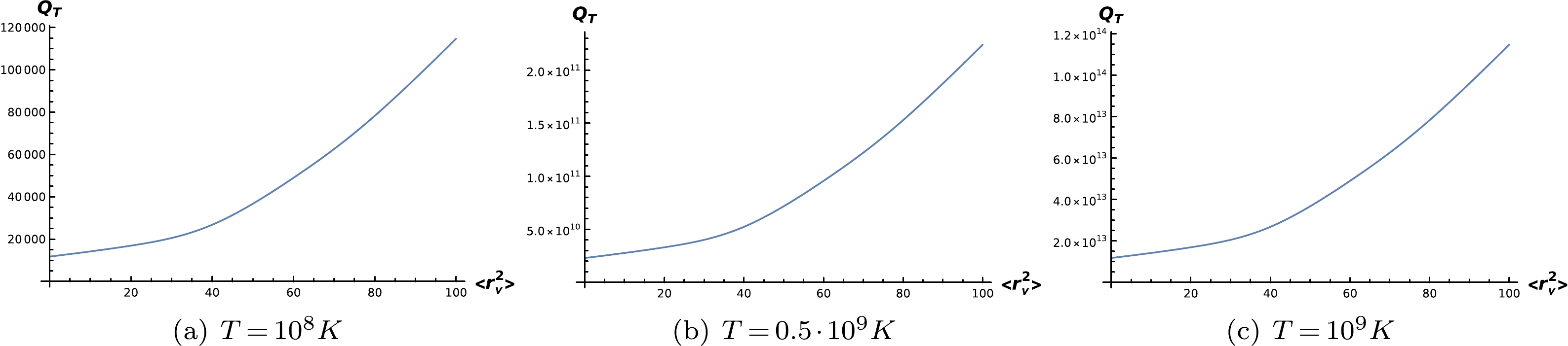
Figure 2. (color online) Energy loss rates (
$\mathcal{Q}_ \mathcal{T}\rm (erg/cm^3 \cdot s)$ ) versus the charge radius ($< r_\nu^2 > \times (10^{-32}\rm ~cm^2$ ) for different values of the temperature (T) in the nondegenerate case.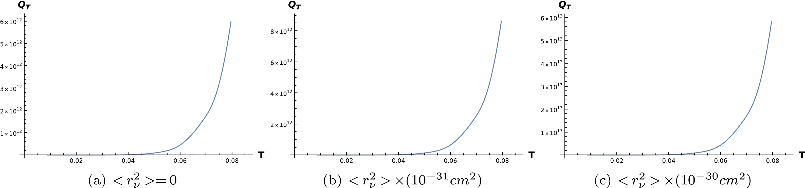
Figure 3. (color online) Energy loss rates (
$\mathcal{Q}_ \mathcal{T}\rm (erg/cm^3 \cdot s)$ ) versus temperature ($T(10^9\rm K)$ ) for different values of the charge radius ($ <r_\nu^2> $ ) in the nondegenerate case.Finally, in Fig. 4, we plot a 3-D graph of
$ \ln(\mathcal{Q}_ \mathcal{T}) $ for different values of temperatures and charge radii. Similar to the results summarized in Tables 1–3, it is observed that the change in the total energy loss rate is different in the degenerate case compared to that in the two other cases, owing to the division of photon energy into neutrino and anti-neutrino pair energy.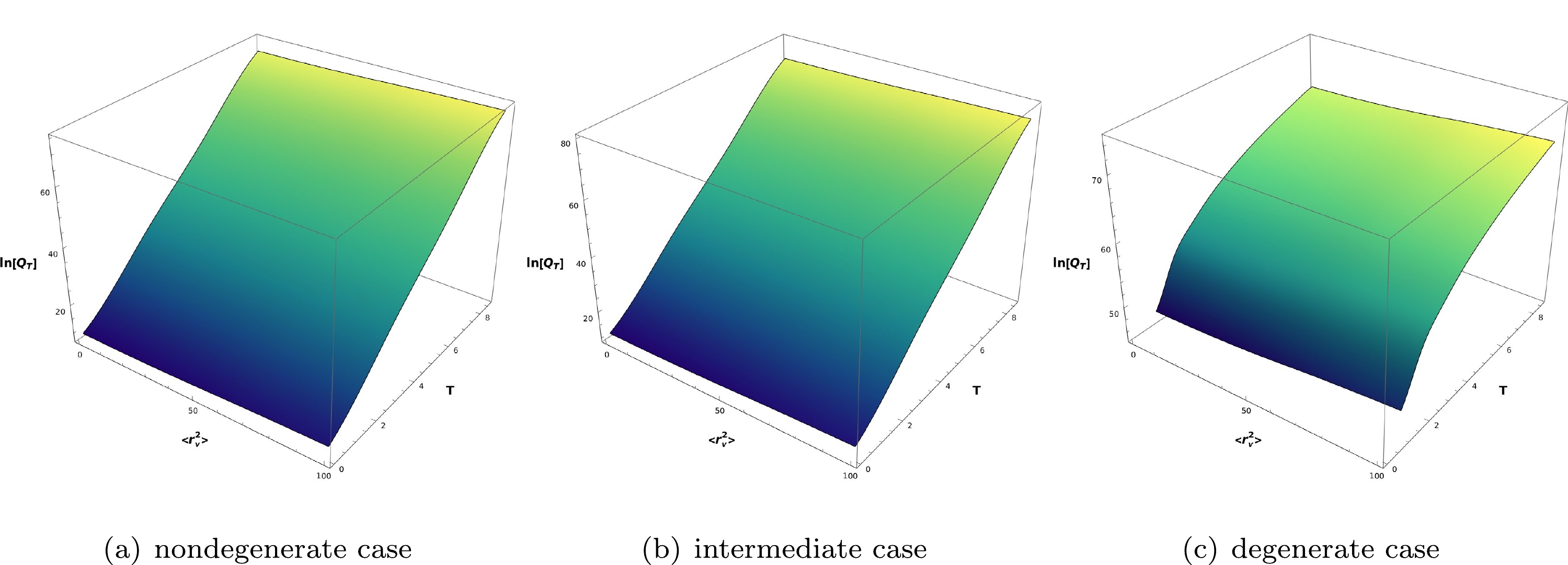
Figure 4. (color online) Logarithm graphs of the total energy loss rate (
$\ln( \mathcal{Q}_ \mathcal{T}\rm (erg/cm^3 \cdot s))$ ) versus the charge radius and temperature ($T(10^9\rm K)$ ) for$< r_\nu^2 > \times (10^{-32}\rm cm^2)$ in (a) and$< r_\nu^2 > \times (10^{-30}\rm cm^2)$ in (b) and (c). -
In summary, in this study, we calculated the energy loss rates associated with the photo-neutrino process considering neutrino charge radius (or anapole moment) effects. The results indicate that the contribution of the charge radius changes the result by approximately 10 %. The contribution of the neutrino magnetic moment is negligible. We observe that if the neutrino magnetic moment is of the following order
$\mu_\nu = 10^{-6} \mu_{\rm B}$ , the indicated term has a dominant effect, and the contribution should be considered. However, this value is still greater than the magnetic moment of a tau-neutrino.
Stellar energy loss rates associated with photoneutrino processes in the minimal extension of the standard model
- Received Date: 2022-12-09
- Available Online: 2023-04-15
Abstract: Using the minimal extension of the standard model and considering the charge radius and the anapole moments of a neutrino, we derive analytical expressions for the stellar energy loss rates associated with the production of a neutrino pair


 DownLoad: