


 Abstract
 HTML
HTML Reference
 Related
 PDF
PDF


-
CP violation plays an important role in the study of weak interactions in elementary particle physics and in attempts to explain the dominance of matter over antimatter in the present universe. The first evidence of CP violation was observed in neutral kaon decays [1], then in the B meson decays [2, 3], and recently in D meson decays [4]. However, no significant observation has yet been reported in baryonic decays, except in beauty baryonic decays [5–8]. Charmed baryonic decays have been used to study weak interactions and provide a unique laboratory to test CP symmetry. To probe the charmed baryonic decay mechanism, parity violation was predicted by calculating decay asymmetry parameters. This has been investigated using a large variety of models, such as the pole model, current algebra, SU(3) flavor symmetry, and perturbative QCD [9–17]. The decays of charmed baryons, for example,
$ \Lambda_c $ , receive contributions from both W emission and W exchange diagrams. Owing to the fact that W emission can be factored out from the short range process, its contribution can be determined from experiments. However, the W exchange contribution, for example, in the Cabibbo-favored decay process$ {{\Lambda_c^+}} \to\phi p $ via the quark transition$ c\to s\bar s u $ , and the singly Cabibbo-suppressed decay process$ {{\Lambda_c^+}} \to \omega p $ via the transition$ c\to ud\bar d $ or scattering$ cd \to ud $ , is uncertain in the model predictions. Precise measurement of the asymmetry parameters will shed light on the charmed baryon decay mechanism.Recently, the branching fraction of
$ {{\Lambda_c^+}} \to \omega p $ was measured using$ pp $ collision data collected at the LHCb experiment [18] and$ {e^+e^-} $ collision data collected at the Belle detector [19]. Using 567$ \mathrm{pb}^{-1} $ data events taken at$ \sqrt{s}=4.599 $ GeV, the branching fraction of$ {{\Lambda_c^+}} \to \phi p $ was measured by the BESIII Collaboration [20]. However, these statistics were limited to measuring decay asymmetry parameters. The decay rate has been intensively investigated by many groups, such as dynamics calculations [16, 21–23] and SU(3) flavor symmetry [17, 24– 28]. The branching fraction of$ {{\Lambda_c^+}} \to \omega p $ was predicted as$ (0.63\pm 0.34)\times 10^{-3} $ by Geng [27],$ (11.4\pm 5.4)\times 10^{-3} $ by Hsiao [28] based on SU(3) symmetry, and$10^{-4}\sim 10^{-2}$ by Singer [23] based on dynamics calculations. A large theoretical uncertainty still exists in the calculation of W exchange diagrams.It is well known that parity violation has been observed in the hyperon of hadronic decays, for example,
$ \Lambda\to p\pi^- $ , in which weak interactions do not conserve the parity. Hence, the decay takes place via both the parity allowed P wave and the parity violated S wave for the two-body final states. The interference between the two waves gives rise to the asymmetry angular distribution, which is characterized by an intrinsic asymmetry parameter, for example,$ \alpha_\Lambda = 0.750\pm 0.009\pm 0.004 $ [29] for$ \Lambda\to p\pi^- $ .Similarly, the asymmetry parameters of
$\Lambda_c\to Vp\; (V= \phi,\omega)$ decays partly encode the weak interactions in$ \Lambda_c $ decays. We define the parameters with helicity amplitudes$ B_{\lambda_3,\lambda_4} $ , where$ \lambda_3 $ and$ \lambda_4 $ are the helicity values of vector mesons and protons, respectively. The nonzero value of the helicity amplitude assumes four configurations, namely,$ B_{1,{{1\over 2}}},\; B_{-1,-{{1\over 2}}},\; B_{0,{{1\over 2}}} $ , and$ B_{0,-{{1\over 2}}} $ . If parity is conserved in the decay, the amplitudes of the four components are reduced to two independent amplitudes with the relations$ B_{1,{{1\over 2}}}=B_{-1,-{{1\over 2}}},\; B_{0,{{1\over 2}}}=B_{0,-{{1\over 2}}} $ . In other words, if$ B_{1,{{1\over 2}}}\neq B_{-1,-{{1\over 2}}} $ and/or$ B_{0,{{1\over 2}}}\neq B_{0,-{{1\over 2}}} $ , parity violation is assumed to take place in the decay. We introduce three parameters to identify the possible effects due to parity violation in$ \Lambda_c\to V p $ decays,$ \begin{aligned}[b] \alpha_{\phi p}=&\frac{|B_{1,{{1\over 2}}}|^2-|B_{-1,-{{1\over 2}}}|^2} {|B_{1,{{1\over 2}}}|^2+|B_{-1,-{{1\over 2}}}|^2},\\ \beta_{\phi p}=&\frac{|B_{0,{{1\over 2}}}|^2-|B_{0,-{{1\over 2}}}|^2} {|B_{0,{{1\over 2}}}|^2+|B_{0,-{{1\over 2}}}|^2}, \\ \gamma_{\phi p}=&\frac{|B_{1,{{1\over 2}}}|^2+|B_{-1,-{{1\over 2}}}|^2}{|B_{0,{{1\over 2}}}|^2+|B_{0,-{{1\over 2}}}|^2}. \end{aligned} $

(1) Obviously, the nonzero values of
$ \alpha_{\phi p} $ and$ \beta_{\phi p} $ imply P parity violation in this decay, which is more straightforward than the definition of asymmerty parameters with two partial wave amplitudes introduced by Lee-Yang [30].$ \gamma_{\phi p} $ represents the relative magnitude of these two types of amplitudes. The two sets of parameter definitions can be converted into each other via the relationship between the helicity decay amplitude and the partial-wave amplitude with the Clebsch-Gordan coefficient.Experimentally, there is another definition for the parameterization of parity asymmetry analogous to the case of
$ \Lambda_b \to \phi p $ [31],$ \Lambda_{\phi p}={|B_{1,{{1\over 2}}}|^2-|B_{-1,-{{1\over 2}}}|^2+|B_{0,{{1\over 2}}}|^2-|B_{0,-{{1\over 2}}}|^2\over |B_{1,{{1\over 2}}}|^2+|B_{-1,-{{1\over 2}}}|^2+|B_{0,{{1\over 2}}}|^2+|B_{0,-{{1\over 2}}}|^2}. $

(2) If we choose the amplitude normalization as
$ |B_{1,\frac{1}{2}}|^2=1 $ , it relates to the previous parameterization via$ \Lambda_{\phi p}=\frac{\beta_{\phi p}+\alpha_{\phi p}\gamma_{\phi p}}{1+\gamma_{\phi p}}, $

(3) where the asymmetry parameter
$ \Lambda_{\phi p} $ does not provide detailed asymmetric information because it depends on the three independent parameters$ \alpha_{\phi p}, \beta_{\phi p} $ , and$ \gamma_{\phi p} $ . We parameterize the amplitude in terms of magnitude and phase angle, for example,$B_{\lambda_{3},\lambda_4}=b_{\lambda_{3},\lambda_4}{\rm e}^{{\rm i} \xi_{\lambda_{3},\lambda_4}}$ , which leads to$ \begin{aligned}[b] b_{1,{{1\over 2}}}^2=&1,\\ b_{-1,-{{1\over 2}}}^2=&{1-\alpha_{\phi p}\over 1+\alpha_{\phi p}},\\ b_{0,{{1\over 2}}}^2=&{1+\beta_{\phi p}\over (1+\alpha_{\phi p})\gamma_{\phi p}},\\ b_{0,-{{1\over 2}}}^2=&{1-\beta_{\phi p}\over (1+\alpha_{\phi p})\gamma_{\phi p}}. \end{aligned} $

(4) In this paper, we use Eq. (1) to identify parity violation effects in the decay
$ \Lambda_c \to pV (V=\omega, \phi) $ .Assuming that CP symmetry is a good approximation in the
$ {{\Lambda_c^+}} $ and$ {{\bar\Lambda_c^-}} $ decays, we have the asymmetry parameters for the conjugate$ {{\bar\Lambda_c^-}} $ decay as$ \begin{array}{*{20}{l}} \alpha_{\phi p}=-\overline{\alpha_{\phi \bar{p}}},\; \; \; \beta_{\phi {p}}=-\overline{\beta_{\phi \bar{p}}},\; \; \; \gamma_{\phi {p}}=\overline{\gamma_{\phi \bar{p}}}. \end{array} $

(5) Thus, we only formulate the
$ \Lambda_c^+ $ decays as follows. Experimentally, extraction of these parameters can be performed by fitting the data events with the joint angular distributions, as in Refs. [32, 33]. Once more data is available, the two conjugate decays can be studied separately for further testing of CP symmetry in charmed baryonic decays. For example, if the experimental results show that any of the equations in Eq. (5) are not valid, we can conclude that CP is violated in this decay. Compared with the traditional method of measuring CP violation, as used in [34], our parameters provide more detailed information on CP violation. -
Let us first consider the decay process
$ {{\Lambda_c^+}}\to V p $ , where V denotes ϕ or ω, and the subsequent decays$ \phi\to K^+K^- $ and$ \omega\to\pi^+\pi^-\pi^0 $ . We formulate the decays using the helicity formalism, from which the asymmetry decay parameters are introduced and can be extracted by fitting the data events with the functions of angular distributions.Helicity angles for
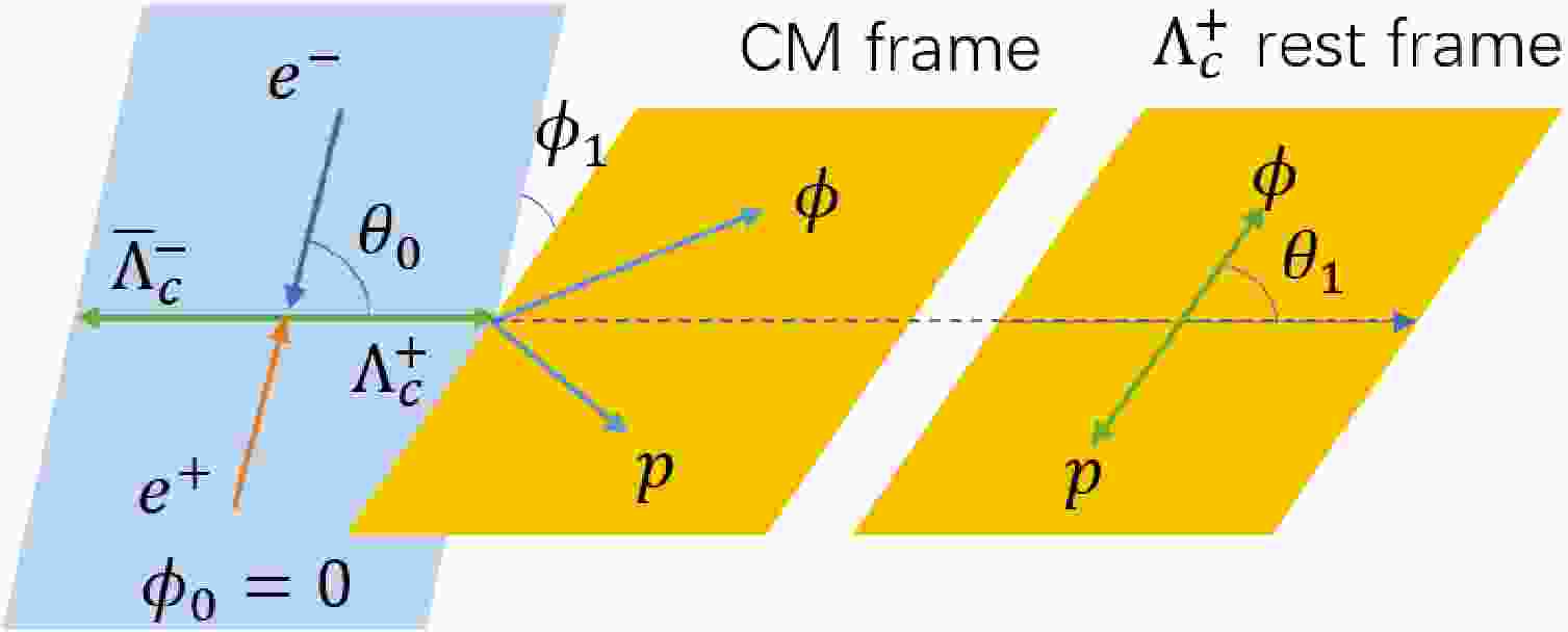
$ {{\Lambda_c^+}}\to \phi p, \phi \to K^+K^- $ are defined as shown in Fig. 1, and the corresponding helicity amplitudes are tabulated in Table 1. For the strong decay, which meets the parity conservation, we have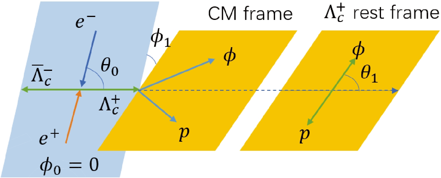
Figure 1. (color online) Definition of the helicity frame at the BESIII experiment.
decay helicity angle helicity amplitude $ {{\Lambda_c^+}}(\lambda_1)\to\phi(\lambda_3)p(\lambda_4) $ 

( $ \theta_1,\phi_1 $ )

$ B_{\lambda_3,\lambda_4} $ 

$ \phi(\lambda_3)\to K^+K^- $ 

( $ \theta_2,\phi_2 $ )

C Table 1. Definition of
$ \phi \to K^+ K^- $ decays, helicity angles, and amplitudes, where$ \lambda_i $ indicates the helicity values for the corresponding hadron.$ \begin{array}{*{20}{l}} F^J_{\lambda_m, \lambda_n}=\eta\eta_1\eta_2(-1)^{J-s_1-s_2} F^J_{-\lambda_m, -\lambda_n}, \end{array} $

(6) where J is the spin of the mother particle,
$ s_i $ is the spin of daughter particles,$ \eta_i $ is the intrinsic parity of each particle, and$ \lambda_i $ indicates the helicity values [35]. For this decay, we have$ J=1,~ s_1=s_2=0 $ ,$ \eta=-1,~ \eta_1=\eta_2=-1 $ , and the helicity of the kaon is zero, with only one independent amplitude, which is labeled as C.For the
$ \omega \to \pi^+\pi^-\pi^0 $ decay, the helicity angles and amplitudes are defined in the same way as shown in Table 2. If the P parity is conserved in three-body systems, we have the following symmetry relation for helicity amplitudes:decay helicity angle helicity amplitude $ {{\Lambda_c^+}}(\lambda_1)\to\omega(\lambda_3)p(\lambda_4) $ 

( $ \theta_1,\phi_1 $ )

$ B_{\lambda_3,\lambda_4} $ 

$ \omega(\lambda_3)\to \pi^+\pi^-\pi^0 $ 

( $ \alpha,\beta,\gamma $ )

C Table 2. Definition of
$ \omega \to \pi^+ \pi^- \pi^0 $ decays, helicity angles, and amplitudes.$ \begin{array}{*{20}{l}} C^J_\mu(E_i \lambda_i)=\eta\eta_1\eta_2\eta_3(-1)^{s_1+s_2+s_3+\mu}C^J_\mu(E_i -\lambda_i), \end{array} $

(7) where J is the spin of the mother particle,
$ s_1,s_2,s_3 $ are for the final particles, μ is the eigenvalue of J in the body-fixed z-axis, and$ E_i $ and$ \lambda_i $ are the energy and helicity of the three particles [35]. For the pion, the helicity is zero; therefore, we can have$ \begin{array}{*{20}{l}} C^1_1(E_i)=-C^1_1(E_i)=0,\; \; \; C^1_{-1}(E_i)=-C^1_{-1}(E_i)=0, \end{array} $

(8) with only one helicity amplitude
$ C^1_0(E_i) $ , and we also denote it as C, whose form is no different from ϕ in joint helicity decay amplitudes. -
The spin density matrix (SDM) encodes all polarization information of a particle in a decay and can be used to clearly demonstrate the spin and polarization transfer in sequential decays [36]. The SDM of spin-
$ 1\over2 $ particles, such as$ {{\Lambda_c^+}} $ , can be expressed as$ \rho={{\mathit{\boldsymbol{\boldsymbol{\mathcal{P}_0}}}}\over2}(\mathit{\boldsymbol{I}}+\mathit{\boldsymbol{\mathcal{P}}}\cdot\mathit{\boldsymbol{\sigma}}), $

(9) where
$ \mathit{\boldsymbol{\mathcal{P}_0}} $ is the unpolarized cross section,$ \mathit{\boldsymbol{\mathcal{P}}} $ is the polarized vector,$ \mathit{\boldsymbol{I}} $ is a 2$ \times $ 2 unit matrix, and$ \mathit{\boldsymbol{\sigma}} $ is the Pauli matrix. Specifically, we can write the SDM of$ {{\Lambda_c^+}} $ as$ \rho^{{\Lambda_c^+}}={{\mathit{\boldsymbol{\mathcal{P}_0}}}\over2}{\left(\begin{array}{cc}1+\mathit{\boldsymbol{\mathcal{P}_z}}&\mathit{\boldsymbol{\mathcal{P}_x}}-{\rm i}\mathit{\boldsymbol{\mathcal{P}_y}} \\\mathit{\boldsymbol{\mathcal{P}_x}}+{\rm i} \mathit{\boldsymbol{\mathcal{P}_y}}& 1-\mathit{\boldsymbol{\mathcal{P}_z}}\end{array}\right)}, $

(10) where
$ \mathit{\boldsymbol{\mathcal{P}_x}} $ and$ \mathit{\boldsymbol{\mathcal{P}_y}} $ are the transverse polarization, and$ \mathit{\boldsymbol{\mathcal{P}_z}} $ is the longitudinal polarization in the coordinate system, as defined in Fig. 1.Using the SDM of
$ {{\Lambda_c^+}} $ , the elements of the ϕ or ω SDM can be calculated as$ \begin{aligned}[b]& \rho^\phi_{\lambda_3,\lambda_3}\propto\sum\limits_{\lambda_{1},\lambda_{1}^{'},\lambda_4}{\rho^{{{\Lambda_c^+}}}_{\lambda_{1},\lambda_{1}^{'}}}D^{{1\over2}*}_{\lambda_{1},\lambda_{3}-\lambda_{4}}(\phi_1,\theta_1,0)\\ & D^{{1}}_{\lambda_{1}^{'},\lambda_{3}^{'}-\lambda_{4}}(\phi_1,\theta_1,0)B_{\lambda_{3},\lambda_{4}}B_{\lambda_{3}^{'},\lambda_{4}}^{*}. \end{aligned} $

(11) Here,
$ D^{J}_{\lambda_i,\lambda_k} $ is the Wigner-D function. The results of this calculation are listed in Appendix A.However, the SDM can be rewritten in terms of the real multipole parameter
$ r^L_M $ , which is defined as$ r^L_M=\mathrm{Tr}[\rho^\phi \cdot Q^L_M], $

(12) where
$ Q^L_M $ is a series of Hermitian basis matrices and can be calculated using the method in Ref. [37]. Tr denotes taking a trace of the matrix. The L-rank index runs from 1 to 2J, and M is regarded as an integer number that runs from –L to L. For a spin-J particle, the SDM can be expressed as$ \rho={{r^0_0}\over{2J+1}}\left(\mathit{\boldsymbol{I}}+2J\sum\limits_{L=1}^{2J}\sum\limits_{M=-L}^{L}r^L_{M}Q^L_{M}\right), $

(13) where
$ \mathit{\boldsymbol{I}} $ denotes a unit matrix with a dimension of$ 2J+1 $ , and$ r^0_0 $ corresponds to the unpolarized decay rate with$ r^0_0 = \mathrm{Tr}\rho $ . We then get the SDM of ϕ as$ \rho^\phi=\frac{{r}^0_0}{3}\left( \begin{array}{ccc} 1+\sqrt{3} {r}^1_0+{r}^2_0 &\sqrt{\dfrac{3}{2}}(-{\rm i} {r}^1_{-1} + {r}^1_1 -{\rm i}{r}^2_{-1}+ {r}^2_1) & \sqrt{3}(-{\rm i}{r}^2_{-2}+{r}^2_2) \\ \sqrt{\dfrac{3}{2}}( {\rm i}{r}^1_{-1} + {r}^1_1 +{\rm i}{r}^2_{-1} +{r}^2_1 ) &1-2 {r}^2_0 &\sqrt{\dfrac{3}{2}}(-{\rm i} {r}^1_{-1} +{r}^1_1 +{\rm i} {r}^2_{-1}-{r}^2_1)\\ \sqrt{3}({\rm i}{r}^2_{-2} + {r}^2_2) &\sqrt{\dfrac{3}{2}}({\rm i} {r}^1_{-1} +{r}^1_1 -{\rm i}{r}^2_{-1} -{r}^2_1 ) &1-\sqrt{3} {r}^1_0 +{r}^2_0 \end{array} \right). $

(14) The multipole parameters can be related to the polarization expressions in Appendix B.
In the equations in these appendices, we reformulate the helicity amplitude for
$ {{\Lambda_c^+}}\to p\phi $ in terms of magnitude and phase angles, namely,$ \begin{aligned}[b] B_{\lambda_3,\lambda_4}=&b_{\lambda_3,\lambda_4}{\rm e}^{{\rm i}\xi_{\lambda_3,\lambda_4}},\\\Delta_{01}=&\xi _{0,\frac{1}{2}}-\xi_{1,\frac{1}{2}},\\ \Delta_{10}=&\xi _{-1,-\frac{1}{2}}-\xi _{0,-\frac{1}{2}}, \end{aligned} $

(15) and the modulus
$ b_{\lambda_{3},\lambda_4} $ relates to the asymmetry parameters according to Eq. (4). -
By making use of the individual helicity amplitude of the decay in a chain, namely,
$ {{\Lambda_c^+}}\to\phi p $ and$ \phi\to K^+K^- $ , the joint angular distribution of this process is expanded in terms of the multipole parameters$ r^L_M $ . The square of the amplitude$ |C|^2 $ can be normalized to one, which reads as$ \begin{aligned}[b] \mathcal{W}(\theta_0,\theta_1,\theta_2,\phi_1,\phi_2)\propto&\sum\limits_{\lambda_3,\lambda_3^{'}}\rho^\phi_{\lambda_3,\lambda_3^{'}}D^{1*}_{\lambda_3,0}D^{1}_{\lambda_3^{'},0}|C|^2\\ =&-\frac{1}{6} r^0_0 \left\{2 \sqrt{3} \mathrm{\sin}2\theta_2[r^2_{-1} \mathrm{\sin} \phi_2\right.\\ & +r^2_1 \mathrm{\cos} \phi_2]+3 r^2_0 \mathrm{\cos}2\theta_2+r^2_0-2\left.\right\}. \end{aligned} $

(16) The helicity amplitude prescription of the
$\omega \to \pi^+\pi^-\pi^0$ process is different from that of the$ \phi \to K^+ K^- $ process. In the$ \omega \to \pi^+\pi^-\pi^0 $ decay, the Euler angles$ (\alpha, \beta, \gamma) $ are used, which describe the rotation necessary for the ω rest frame to overlap the helicity frame formed by the three pion momenta. The deduction of angular distribution is similar to that of the ϕ decay. The result is$ \begin{aligned}[b] \mathcal{W}(\theta_0,\theta_1,\phi_1,\alpha,\beta,\gamma)\propto& -\frac{1}{6} r^0_0 \left\{2 \sqrt{3} \mathrm{\sin}2\beta [r^2_{-1} \mathrm{\sin} \alpha\right.\\ &+r^2_1 \mathrm{\cos} \alpha]+3 r^2_0 \mathrm{\cos}2\beta +r^2_0-2\left.\right\}. \end{aligned} $

(17) -
The helicity angles in the
$ \phi \to K^+ K^- $ process can be used to form a polarization observable to describe the relevant multipole parameters [32]. We give the first moments of the Wigner D-function below to present the ϕ polarization effects (the ω decay is nearly the same).$ \langle \mathrm{\cos}2\theta_2\rangle =-{1\over 15}(5+8r^2_0), $

(18) $\langle \mathrm{\sin}2\theta_2\mathrm{\cos}\phi_2 \rangle =-{4\over 5\sqrt 3}r^2_1, $

(19) $ \langle \mathrm{\sin}2\theta_2\mathrm{\sin}\phi_2 \rangle =-{4\over 5\sqrt 3}r^2_{-1}. $

(20) -
Let us consider the cascade decay, that is,
${e^+e^-}\to \gamma^*(M_0) \to {{\Lambda_c^+}}(\lambda_{1})\;{{\bar\Lambda_c^-}}(\lambda_{2}),~\; {{\Lambda_c^+}}(\lambda'_{1}) \to \phi(\lambda_3)\,p(\lambda_4),$ $\phi(\lambda_3)\to K^+K^-$ , which can be studied at the BESIII experiment,$pp \;\to\; \Lambda_b^0X,~~~ {{\Lambda}_b^0}(M_0) \;\to\; {{\Lambda_c^+}}(\lambda_1)\pi^-, ~~~ {{\Lambda_c^+}}(\lambda_1^{'}) \;\to\; \phi(\lambda_3) p(\lambda_4),$ $\phi(\lambda_3')\to K^+K^-$ , which can be studied at the LHCb experiment, where the helicity values, that is,$M_0,~ \lambda_i$ and$ \lambda'_j $ , are indicated in the parentheses for the corresponding particles. Table 3 contains the definitions of helicity angles and amplitudes in producing$ {{\Lambda_c^+}} $ at the BESIII and LHCb experiments.decay helicity angle helicity amplitude $ \gamma^*(M_0)\to{{\Lambda_c^+}}(\lambda_1){{\bar\Lambda_c^-}}(\lambda_2) $ 

( $ \theta_0,\phi_0 $ )

$ A_{\lambda_1,\lambda_2} $ 

$ \Lambda_b^0(M_0)\to{{\Lambda_c^+}}(\lambda_1)\pi^- $ 

( $ \theta_0,\phi_0 $ )

$ A_{\lambda_1} $ 

Table 3. Definition of helicity angles and amplitudes in experiments.
-
At the BESIII experiment, baryon pairs are produced from unpolarized beam
$ {e^+e^-} $ collisions [38], and the decay chain is${e^+e^-}\to{{\Lambda_c^+}}{{\bar\Lambda_c^-}},~ {{\Lambda_c^+}}\to\phi p$ ,$ \phi\to K^+K^- $ , and as shown in Fig. 1. In this decay, the polar and azimuthal angles are defined as follows:$ \begin{aligned}[b] \phi_0=&0,\; \; \; \; \; \; \; \; \; \; \; \mathrm{\cos}\theta_0=\frac{\vec{p}_{e^+}\cdot{\vec{p}_{{\Lambda_c^+}}}}{\lvert\vec{p}_{e^+}\lvert\cdot\lvert\vec{p}_{{\Lambda_c^+}}\rvert},\\ \mathrm{\cos}\phi_1=&|\vec{n}_1\cdot{\vec{n}_2}|, \; \; \; \mathrm{\cos}\theta_1=\frac{\vec{p}_\phi\cdot{\vec{p}_{{\Lambda_c^+}}}}{\lvert\vec{p}_\phi\lvert\cdot\lvert\vec{p}_{{\Lambda_c^+}}\rvert},\\ \mathrm{\cos}\phi_2=&|\vec{n}_2\cdot{\vec{n}_3}|, \; \; \; \mathrm{\cos}\theta_2=\frac{\vec{p}_{K^+}\cdot{\vec{p}_\phi}}{\lvert\vec{p}_{K^+}\lvert\cdot\lvert\vec{p}_\phi\rvert}, \end{aligned} $

(21) where
$ \vec{p} $ denotes the momentum of each particle in the rest frame of their respective parent particles, and$ \vec{n}_i $ is the normal vector defined as$ \begin{aligned}[b] \vec{n}_1=&\frac{\vec{p}_{e^+}\times{\vec{p}_{{\Lambda_c^+}}}}{\lvert\vec{p}_{e^+}\lvert\cdot\lvert\vec{p}_{{\Lambda_c^+}}\rvert\cdot{\mathrm{\sin}\theta_0}}, \; \; \; \vec{n}_2=\frac{\vec{p}_{{{\Lambda_c^+}}}\times{\vec{p}_\phi}}{\lvert\vec{p}_{{{\Lambda_c^+}}}\lvert\cdot\lvert\vec{p}_\phi\rvert\cdot{\mathrm{\sin}\theta_1}},\\ \vec{n}_3=&\frac{\vec{p}_{\phi}\times{\vec{p}_{K^+}}}{\lvert\vec{p}_{\phi}\lvert\cdot\lvert\vec{p}_{K^+}\rvert\cdot{\mathrm{\sin}\theta_2}}. \end{aligned} $

(22) For example,
$ \theta_1 $ is the polar angle between the momentum of ϕ and$ {{\Lambda_c^+}} $ in the$ {{\Lambda_c^+}} $ rest frame, and$ \phi_2 $ is the azimuthal angle between the$ {{\Lambda_c^+}}\to\phi p $ decay plane and the$ \phi\to K^+K^- $ decay plane, as shown in Fig. 1.The SDM of
$ {{\Lambda_c^+}} $ for the BESIII experiment can be formulated as$ \begin{aligned}[b] \rho^{{\Lambda_c^+}}_{\lambda_1,\lambda_1^{'}}\propto&\sum\limits_{{M_0},\lambda_2}{\rho^{\gamma^*}_{M_0,M_0^{'}}}D^{1*}_{M_0,\lambda_{1}-\lambda_{2}}(\phi_0,\theta_0,0)\\ &\times D^{{1}}_{M_0^{'},\lambda_{1}^{'}-\lambda_{2}}(\phi_0,\theta_0,0)A_{\lambda_{1},\lambda_{2}}A_{\lambda_{1}^{'},\lambda_{2}}^{*}, \end{aligned} $

(23) where
$ {\rho^{\gamma^*}_{M_0,M_0^{'}}} $ is a diagonal matrix written as$ \dfrac{1}{2}\mathrm{diag}\left\{\right.1,0,1\left.\right\} $ . For the parity conserved decay, the symmetry relation is$ A_{-{{1\over 2}},-{{1\over 2}}}=A_{{{1\over 2}},{{1\over 2}}},\; A_{-{{1\over 2}},{{1\over 2}}}=A_{{{1\over 2}},-{{1\over 2}}}. $

(24) The unpolarized cross section is determined as
$ \mathit{\boldsymbol{\mathcal{P}_0}}=1+\alpha_c\mathrm{\cos}^2\theta_0 $ , where$ \alpha_c $ is the angular distribution parameter for$ {e^+e^-}\to{{\Lambda_c^+}}{{\bar\Lambda_c^-}} $ and is defined as$ \alpha_c={|A_{{{1\over 2}},-{{1\over 2}}}|^2-2|A_{{{1\over 2}},{{1\over 2}}}|^2\over |A_{-{{1\over 2}},{{1\over 2}}}|^2+2|A_{{{1\over 2}},{{1\over 2}}}|^2}. $

(25) The polarization of
$ {{\Lambda_c^+}} $ is calculated to be$ \mathit{\boldsymbol{\mathcal{P}_y}}={\sqrt{1-\alpha_c^2}\mathrm{\sin}(2\theta_0)\mathrm{\sin}\Delta \over 2(1+\alpha_c\mathrm{\cos}^2\theta_0)}, \; \mathit{\boldsymbol{\mathcal{P}_x}}= \mathit{\boldsymbol{\mathcal{P}_z}}=0, $

(26) where Δ is a parameter describing the phase angle difference between the two independent amplitudes of this process, and we leave out the constant
$ |A_{-{{1\over 2}},{{1\over 2}}}|^2+2|A_{{{1\over 2}},{{1\over 2}}}|^2 $ in the$ \mathit{\boldsymbol{\mathcal{P}_0}} $ expression. Consequently,$ {{\Lambda_c^+}} $ may spontaneously have transverse polarization from unpolarized$ {e^+e^-} $ if Δ is nonzero. -
At the LHCb experiment, assuming
$ {{\Lambda_c^+}} $ is produced by the polarized$ {\Lambda}_b^0 $ [39, 40], we write the decay chain as$ {\Lambda}_b^0\to{{\Lambda_c^+}}\pi^-, {{\Lambda_c^+}}\to\phi p $ ,$ \phi\to K^+K^- $ . In this decay chain, we must define two extra angles and a normal vector as$ \begin{aligned}[b] \mathrm{\cos}\phi_0=&\frac{\vec{n}_0\cdot{\vec{n}_1}}{\lvert\vec{n}_0\lvert\cdot\lvert\vec{n}_1\rvert}, \; \; \; \vec{n}_0=\frac{\vec{p}_p\cdot{\vec{p}_{{\Lambda}_b^0}}}{\lvert\vec{p}_p\rvert\cdot{\lvert{\vec{p}_{{\Lambda}_b^0}}\rvert}\mathrm{\sin}\theta},\\ \mathrm{\cos}\theta=&\frac{\vec{p}_{p}\cdot{\vec{p}_{{{\Lambda}}_b^0}}}{\lvert\vec{p}_{p}\lvert\cdot\lvert\vec{p}_{{{\Lambda}}_b^0}\rvert}, \end{aligned} $

(27) where the angles are shown in Fig. 2, compared to
$ {{\Lambda_c^+}} $ produced in the$ {e^+e^-} $ collision. The definitions of other angles are the same as those at the BESIII experiment. Consequently, these quantities can be constructed with the momentum registered in detectors.
Figure 2. (color online) Definition of the helicity frame at the LHCb experiment.
According to Eq. (10), the SDM of
$ {\Lambda}_b^0 $ can be written as$ \rho^{{\Lambda}_b^0}={{\mathit{\boldsymbol{\mathcal{P}}}_0^b}\over2}{\left(\begin{array}{cc}1+\mathit{\boldsymbol{\mathcal{P}}}_z^b&\mathit{\boldsymbol{\mathcal{P}}}_x^b-{\rm i}\mathit{\boldsymbol{\mathcal{P}}}_y^b \\\mathit{\boldsymbol{\mathcal{P}}}_x^b+{\rm i}\mathit{\boldsymbol{\mathcal{P}}}_y^b& 1-\mathit{\boldsymbol{\mathcal{P}}}_z^b\end{array}\right)}. $

(28) The SDM of the decayed particle
$ {{\Lambda_c^+}} $ can be formulated as$ \begin{aligned}[b] \rho^{{\Lambda_c^+}}_{\lambda_1,\lambda_1^{'}}\propto&\sum\limits_{{M_0},\lambda_2}{\rho^{{\Lambda_b^0}}_{M_0,M_0^{'}}}D^{\frac{1}{2}*}_{M_0,\lambda_{1}-\lambda_{2}}(\phi_0,\theta_0,0)\\ &\times D^{\frac{1}{2}}_{M_0^{'},\lambda_{1}^{'}-\lambda_{2}}(\phi_0,\theta_0,0)A_{\lambda_{1}}A_{\lambda_{1}^{'}}^{*}. \end{aligned} $

(29) We define an asymmetry parameter to express the degree of P violation in this weak decay as
$ \alpha_b={|A_{{{1\over 2}}}|^2-|A_{-{{1\over 2}}}|^2\over |A_{{{1\over 2}}}|^2+|A_{-{{1\over 2}}}|^2}, $

(30) and the unpolarized cross section and the polarization of
$ {{\Lambda_c^+}} $ can be expressed as$ \begin{aligned}[b] \mathit{\boldsymbol{\mathcal{P}_0}}=&\frac{\mathit{\boldsymbol{\mathcal{P}_0}}^b}{2}(1+\alpha_b{\mathit{\boldsymbol{\mathcal{P}_z}}^b}\mathrm{\cos}\theta_0+ \alpha_b{\mathit{\boldsymbol{\mathcal{P}_x}}^b}\mathrm{\cos}\phi_0\mathrm{\sin}\theta_0\\ &+ \alpha_b{\mathit{\boldsymbol{\mathcal{P}_y}}^b}\mathrm{\sin}\theta_0\mathrm{\sin}\phi_0),\\ \mathit{\boldsymbol{\mathcal{P}_0}}\mathit{\boldsymbol{\mathcal{P}_x}}=&\frac{\sqrt{1-\alpha_b^2}}{2}\mathit{\boldsymbol{\mathcal{P}_0}}^b(-\mathit{\boldsymbol{\mathcal{P}_y}}^b\mathrm{\cos}\phi_0\mathrm{\sin}\Delta_b\\ &+\mathit{\boldsymbol{\mathcal{P}_x}}^b\mathrm{\cos}\theta_0\mathrm{\cos}\phi_0\mathrm{\cos}\Delta_b-\mathit{\boldsymbol{\mathcal{P}_z}}^b\mathrm{\sin}\theta_0\mathrm{\cos}\Delta_b\\ &+\mathit{\boldsymbol{\mathcal{P}_x}}^b\mathrm{\sin}\phi_0\mathrm{\sin}\Delta_b+\mathit{\boldsymbol{\mathcal{P}_y}}^b\mathrm{\cos}\theta_0\mathrm{\sin}\phi_0\mathrm{\cos}\Delta_b),\\ \mathit{\boldsymbol{\mathcal{P}_0}}\mathit{\boldsymbol{\mathcal{P}_y}}=&\frac{\sqrt{1-\alpha_b^2}}{2}\mathit{\boldsymbol{\mathcal{P}_0}}^b(\mathit{\boldsymbol{\mathcal{P}_y}}^b\mathrm{\cos}\phi_0\mathrm{\cos}\Delta_b\\ &+\mathit{\boldsymbol{\mathcal{P}_x}}^b\mathrm{\cos}\theta_0\mathrm{\cos}\phi_0\mathrm{\sin}\Delta_b-\mathit{\boldsymbol{\mathcal{P}_z}}^b\mathrm{\sin}\theta_0\mathrm{\sin}\Delta_b\\ &-\mathit{\boldsymbol{\mathcal{P}_x}}^b\mathrm{\sin}\phi_0\mathrm{\cos}\Delta_b+\mathit{\boldsymbol{\mathcal{P}_y}}^b\mathrm{\cos}\theta_0\mathrm{\sin}\phi_0\mathrm{\sin}\Delta_b),\\ \mathit{\boldsymbol{\mathcal{P}_0}}\mathit{\boldsymbol{\mathcal{P}_z}}=&\frac{\mathit{\boldsymbol{\mathcal{P}_0}}^b}{2}(\alpha_b+{\mathit{\boldsymbol{\mathcal{P}_z}}^b}\mathrm{\cos}\theta_0+{\mathit{\boldsymbol{\mathcal{P}_x}}^b}\mathrm{\cos}\phi_0\mathrm{\sin}\theta_0\\ &+{\mathit{\boldsymbol{\mathcal{P}_y}}^b}\mathrm{\sin}\theta_0\mathrm{\sin}\phi_0). \end{aligned} $

(31) In these equations,
$ \Delta_b $ is a parameter describing the phase angle difference between the two independent amplitudes of this process, and we ignore the constant$ |A_{{{1\over 2}}}|^2+|A_{-{{1\over 2}}}|^2 $ on the right side of the four equations above. These formulas show the transfer process of polarization in the decay chain. To obtain the polarization effects, we just need to replace the elements of the multipole parameters in Appendix B. -
Sensitivity estimation is indispensable when a data taken proposal is suggested or a physics program is designed before the experiment is carried out. We estimate the statistical sensitivity in terms of the number of observed events for measurement of the
$ \Lambda_c $ decay asymmetry parameter. To increase the sensitivity, information on the full spin transfer through the complete decay chain is used rather than only information from the$ \Lambda_c $ decay. Comparing the joint angular distribution of the two decays of$ \Lambda_c \to \phi p $ and$ \Lambda_c \to \omega p $ , we can see that they take the same form by making the replacement$ (\theta_2,\phi_2)\to (\beta,\alpha) $ in the$ \phi p $ channel. Therefore, we only consider the$ \omega p $ channel in our estimation, with an assumption of different asymmetry parameters, which can be extracted by fitting the normalized angular distribution with adequate data samples. The angular distribution$ \widetilde{\mathcal{W}}(\theta_0,\theta_1,\phi_1,\alpha,\beta,\gamma) $ is defined as$ \widetilde{\mathcal{W}}=\frac{\mathcal{W}(\theta_0,\theta_1,\phi_1,\alpha,\beta,\gamma)}{\int\cdot\cdot\cdot\int\mathcal{W}(\cdot\cdot\cdot)\mathrm{d}\mathrm{\cos}\theta_0\mathrm{d}\mathrm{\cos}\theta_1\mathrm{d}\mathrm{\cos}\beta \mathrm{d}\phi_1 \mathrm{d}\alpha \mathrm{d}\gamma}. $

(32) Here, the denominator plays the role of normalization. For a set of data samples, a likelihood function is defined as
$ L=\prod\limits_{i=1}^{N}\widetilde{\mathcal{W}}(\theta_0,\theta_1,\phi_1,\alpha,\beta,\gamma), $

(33) where N is the number of observed events [41]. Based on the maximum likelihood method, the estimated statistical sensitivity corresponding to each decay parameter is determined by the relative uncertainty
$ \delta(\alpha_{\omega p})=\frac{\sqrt{V(\alpha_{\omega p})}}{|\alpha_{\omega p}|}, $

(34) where
$ V(\alpha_{\omega p}) $ is the variance of the decay parameter$ \alpha_{\omega p} $ , which can be calculated by$ \begin{aligned}[b] V^{-1}(\alpha_{\omega p})=&N\int\frac{1}{\widetilde{\mathcal{W}}}\left[\frac{\partial \widetilde{\mathcal{W}}}{\partial\alpha_{\omega p}}\right]^2\mathrm{d}\mathrm{\cos}\theta_0\mathrm{d}\mathrm{\cos}\theta_1\mathrm{d}\mathrm{\cos}\beta\\ &\times\mathrm{d}\phi_1\mathrm{d}\alpha \mathrm{d}\gamma. \end{aligned} $

(35) The other two parameters,
$ \delta_{\beta_{\omega p}} $ and$ \delta_{\gamma_{\omega p}} $ , are defined analogously to Eqs. (34) and (35).To explore the dependence of sensitivity on the signal yields N produced at the
$ {e^+e^-} $ collider experiment, we compute the value of$ \delta(\alpha_{\omega p}) $ by taking the parameters as$ \begin{aligned}[b] \alpha_{c}=&0.2,\; \; \; \beta_{\omega p}=0.1,\; \; \; \gamma_{\omega p}=0.5,\\ \Delta=&\frac{\pi}{3},\; \; \; \; \Delta_{01}=\frac{\pi}{4},\; \; \; \; \Delta_{10}=\frac{\pi}{6}. \end{aligned} $

(36) We plot the sensitivities of a set of different
$ \alpha_{\omega p} $ values versus the statistics, as shown in Fig. 3. For example, if$ \alpha_{\omega p}=-0.5 $ , we need nearly$300000$ signal events to reach a$5$ % sensitivity. Considering the influence of the background level, detection efficiencies, and a variety of systematic uncertainties, the actual amount of the data sample required in experiments should be larger than what we predict, but the numerical estimation depends on the experimental situation.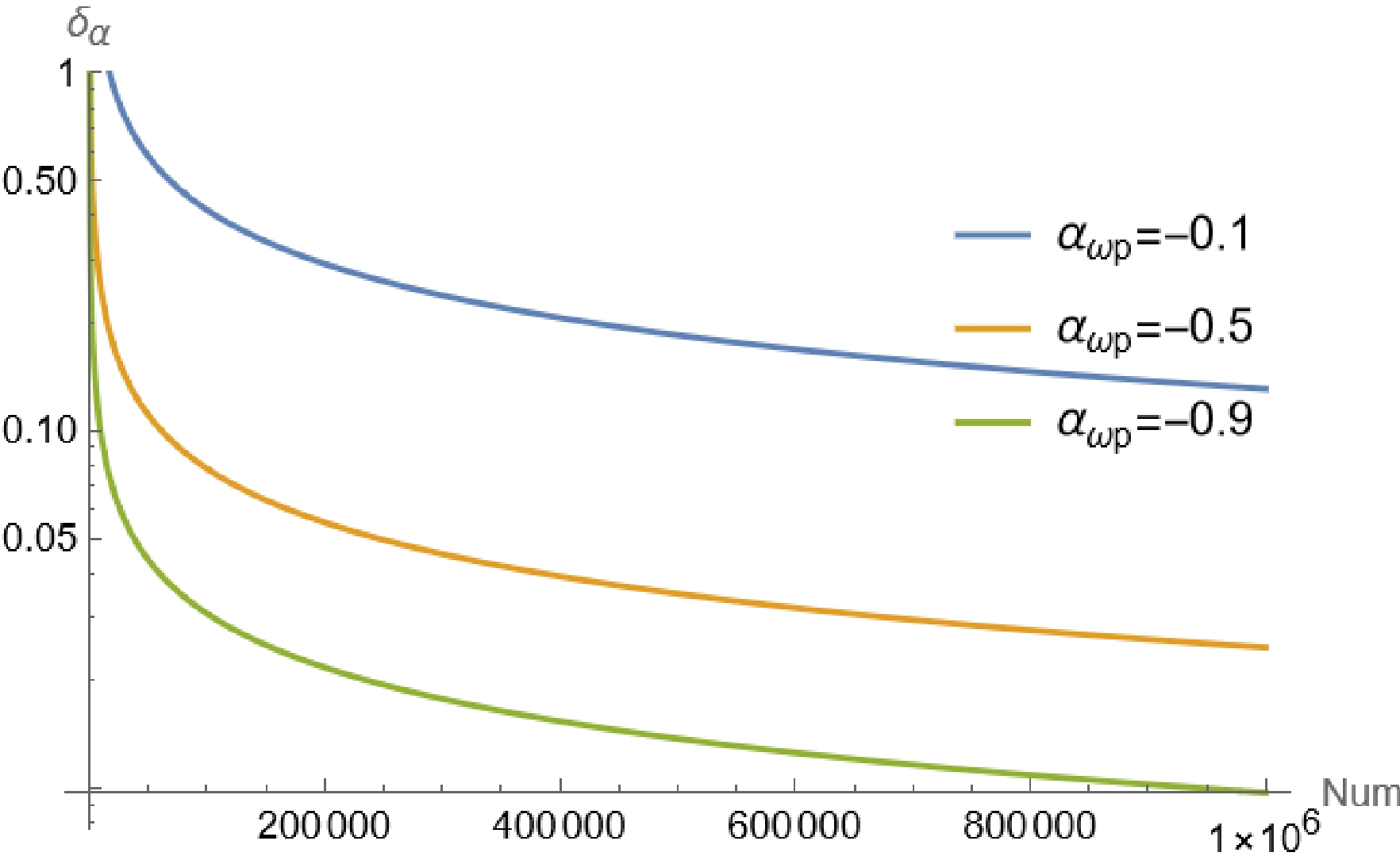
Figure 3. (color online)
$ \alpha_{\omega p} $ sensitivities relative to signal yields N in terms of different values of$ \alpha_{\omega p} $ .By taking the parameters as
$ \begin{aligned}[b] \alpha_{c}=&0.2,\; \; \; \alpha_{\omega p}=-0.5,\; \; \; \gamma_{\omega p}=0.5,\\ \Delta=&\frac{\pi}{3},\; \; \; \; \Delta_{01}=\frac{\pi}{4},\; \; \; \; \; \; \Delta_{10}=\frac{\pi}{6}, \end{aligned} $

(37) and
$ \begin{aligned}[b] \alpha_{c}=&0.2,\; \; \; \alpha_{\omega p}=-0.5,\; \; \; \beta_{\omega p}=0.1,\\ \Delta=&\frac{\pi}{3},\; \; \; \; \Delta_{01}=\frac{\pi}{4},\; \; \; \; \; \; \Delta_{10}=\frac{\pi}{6}, \end{aligned} $

(38) as well as considering different
$ \beta_{\omega p} $ and$ \gamma_{\omega p} $ values, the sensitivities versus statistics are shown in Fig. 4 and Fig. 5.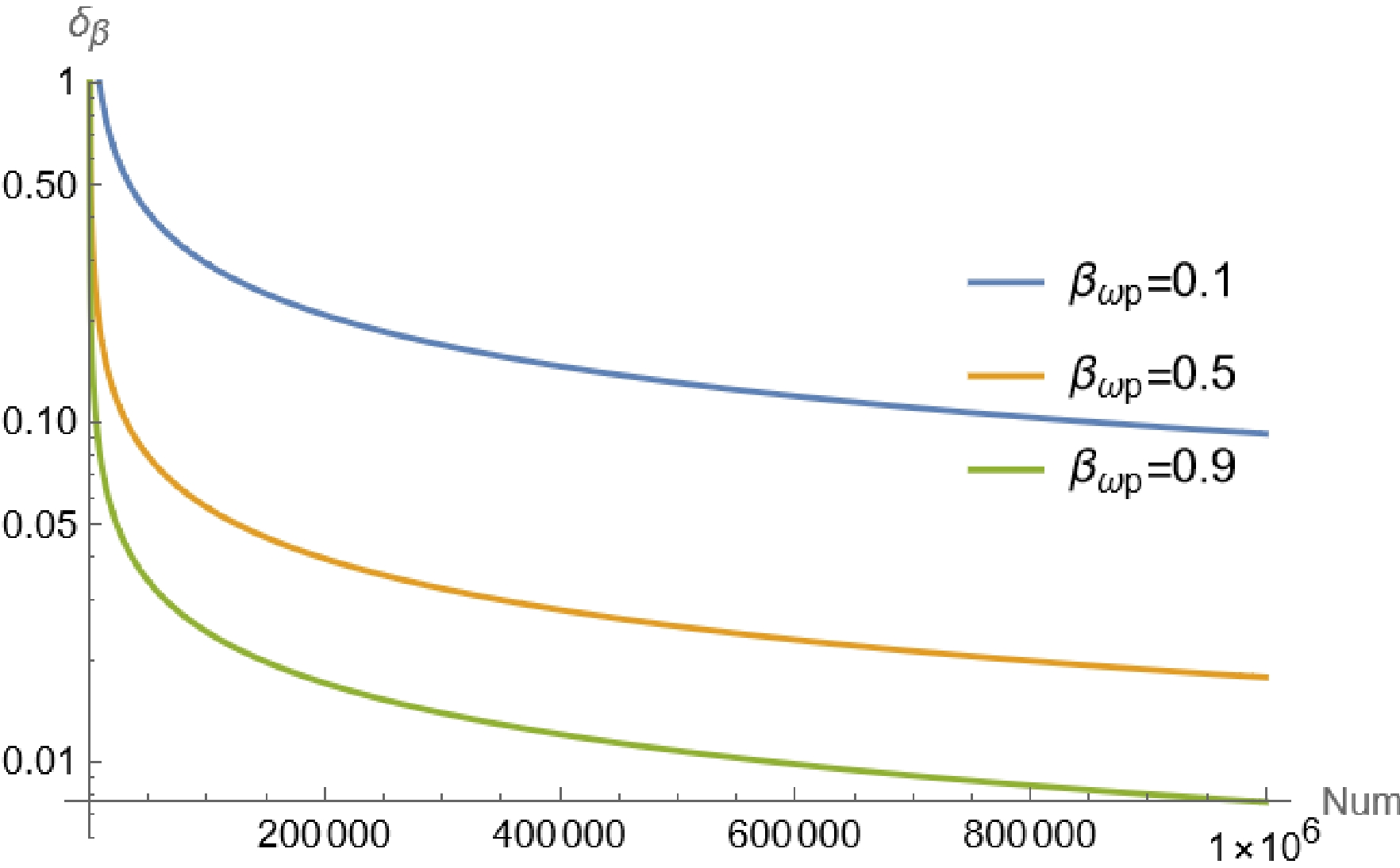
Figure 4. (color online)
$ \beta_{\omega p} $ sensitivities relative to signal yields N in terms of different values of$ \beta_{\omega p} $ .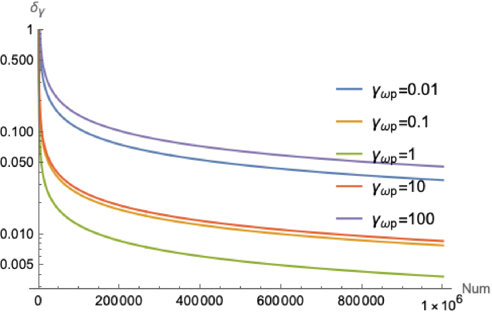
Figure 5. (color online)
$ \gamma_{\omega p} $ sensitivities relative to signal yields N in terms of different values of$ \gamma_{\omega p} $ . -
To study the weak interactions in
$ {{\Lambda_c^+}}\to\phi p $ and$ {{\Lambda_c^+}}\to\omega p $ decays, we formulate asymmetry parameters in these two decays using the helicity amplitudes, and the joint angular distributions are provided. In particular, to investigate the asymmetry parameters at the BESIII and LHCb experiments, we show how the polarization is transferred from the mother particles to the daughter particles. By making use of the full decay chain, the sensitivity of asymmetry parameter measurement is estimated for the channels${{\Lambda_c^+}}\to\omega p, ~ \omega\to\pi^0\pi^+\pi^-$ and$ {{\Lambda_c^+}}\to\phi p, \phi \to K^+ K^- $ . The estimation will be helpful to the design of physics programs in near future facilities, such as the CEPC and STCF. -
$ \begin{aligned}[b] \rho^{\phi}_{1,1}=&\frac{1}{2} \mathit{\boldsymbol{\mathcal{P}_0}} (1+\mathit{\boldsymbol{\mathcal{P}_y}} \mathrm{\sin}\theta _1\mathrm{\sin} \phi_1)b_{1,\frac{1}{2}}^2,\\ \rho^{\phi}_{1,0}=&\frac{1}{2} \mathit{\boldsymbol{\mathcal{P}_0}} \mathit{\boldsymbol{\mathcal{P}_y}} {\rm e}^{-{\rm i} \Delta_{01}} (\mathrm{\cos} \theta_1 \mathrm{\sin} \phi_1-{\rm i} \mathrm{\cos}\phi_1)b_{0,\frac{1}{2}} b_{1,\frac{1}{2}},\\ \rho^{\phi}_{1,-1}=&0,\\ \rho^{\phi}_{0,1}=&\frac{1}{2} \mathit{\boldsymbol{\mathcal{P}_0}} \mathit{\boldsymbol{\mathcal{P}_y}} {\rm e}^{{\rm i} \Delta_{01}} (\mathrm{\cos} \theta _1 \mathrm{\sin} \phi_1+{\rm i} \mathrm{\cos}\phi_1)b_{0,\frac{1}{2}} b_{1,\frac{1}{2}} ,\\ \rho^{\phi}_{0,0}=&\frac{1}{2} \mathit{\boldsymbol{\mathcal{P}_0}}[(1+\mathit{\boldsymbol{\mathcal{P}_y}}\mathrm{\sin}\theta_1\mathrm{\sin}\phi_1)b_{0,\frac{1}{2}}^2\\ &+(1-\mathit{\boldsymbol{\mathcal{P}_y}} \mathrm{\sin}\theta_1 \mathrm{\sin}\phi_1)b_{0,-\frac{1}{2}}^2 ],\\ \rho^{\phi}_{0,-1}=&\frac{1}{2} \mathit{\boldsymbol{\mathcal{P}_0}} \mathit{\boldsymbol{\mathcal{P}_y}} {\rm e}^{-{\rm i} \Delta_{10}} (\mathrm{\cos}\theta_1 \mathrm{\sin}\phi_1-{\rm i} \mathrm{\cos}\phi_1)b_{-1,-\frac{1}{2}} b_{0,-\frac{1}{2}},\\ \rho^{\phi}_{-1,1}=&0,\\ \rho^{\phi}_{1,1}=&\frac{1}{2} \mathit{\boldsymbol{\mathcal{P}_0}} \mathit{\boldsymbol{\mathcal{P}_y}} {\rm e}^{{\rm i} \Delta_{10}} (\mathrm{\cos}\theta_1 \mathrm{\sin}\phi_1+{\rm i} \mathrm{\cos} \phi_1)b_{-1,-\frac{1}{2}} b_{0,-\frac{1}{2}},\\ \rho^{\phi}_{1,1}=&\frac{1}{2} \mathit{\boldsymbol{\mathcal{P}_0}}(1-\mathit{\boldsymbol{\mathcal{P}_y}}\mathrm{\sin}\theta_1 \mathrm{\sin}\phi_1)b_{-1,-\frac{1}{2}}^2. \end{aligned} $

-
$ \begin{aligned}[b] 2r^0_0=&{\mathit{\boldsymbol{\mathcal{P}_0}}}\left\{\right.b_{-1,-\frac{1}{2}}^2 (1-\mathit{\boldsymbol{\mathcal{P}_z}}\mathrm{\cos}\theta_1-\mathit{\boldsymbol{\mathcal{P}_x}}\mathrm{\cos}\phi_1\mathrm{\sin}\theta_1\nonumber\\ &-\mathit{\boldsymbol{\mathcal{P}_y}}\mathrm{\sin}\theta_1\mathrm{\sin}\phi_1)+b_{0,-\frac{1}{2}}^2+b_{0,\frac{1}{2}}^2+b_{1,\frac{1}{2}}^2\nonumber\\ &+[\mathit{\boldsymbol{\mathcal{P}_z}}\mathrm{\cos}\theta_1+\mathrm{\sin}\theta_1(\mathit{\boldsymbol{\mathcal{P}_x}}\mathrm{\cos}\phi_1+\mathit{\boldsymbol{\mathcal{P}_y}}\mathrm{\sin}\phi_1)]\nonumber\\ &\times(b_{0,-\frac{1}{2}}^2-b_{0,\frac{1}{2}}^2+b_{1,\frac{1}{2}}^2)\left.\right\},\\ r^0_0r^1_{-1}=&\frac{1}{2}\sqrt{3\over2}{\mathit{\boldsymbol{\mathcal{P}_0}}}\left\{\right. [\mathrm{\cos}\Delta_{10}(\mathit{\boldsymbol{\mathcal{P}_y}}\mathrm{\cos}\phi_1-\mathit{\boldsymbol{\mathcal{P}_x}}\mathrm{\sin}\phi_1)\\ &+(-\mathit{\boldsymbol{\mathcal{P}_z}}\mathrm{\sin}\theta_1 +\mathrm{\cos}\theta_1(\mathit{\boldsymbol{\mathcal{P}_x}}\mathrm{\cos}\phi_1+\mathit{\boldsymbol{\mathcal{P}_y}}\mathrm{\sin}\phi_1))\\ &\times \mathrm{\sin}\Delta_{10} ]b_{-1,-\frac{1}{2}}b_{0,-\frac{1}{2}} +[\mathrm{\cos}\Delta_{01}(\mathit{\boldsymbol{\mathcal{P}_y}}\mathrm{\cos}\phi_1\\ &-\mathit{\boldsymbol{\mathcal{P}_x}}\mathrm{\sin}\phi_1)+(-\mathit{\boldsymbol{\mathcal{P}_z}}\mathrm{\sin}\theta_1+\mathrm{\cos}\theta_1(\mathit{\boldsymbol{\mathcal{P}_x}}\mathrm{\cos}\phi_1\\ &+\mathit{\boldsymbol{\mathcal{P}_y}}\mathrm{\sin}\phi_1))\mathrm{\sin}\Delta_{01}]b_{0,\frac{1}{2}}b_{1,\frac{1}{2}}\left.\right\},\\ r^0_0r^1_{0}=&\frac{\sqrt{3}}{4}{\mathit{\boldsymbol{\mathcal{P}_0}}}[(-1+\mathit{\boldsymbol{\mathcal{P}_z}}\mathrm{\cos}\theta_1+\mathit{\boldsymbol{\mathcal{P}_x}}\mathrm{\cos}\phi_1\mathrm{\sin}\theta_1\\ &+\mathit{\boldsymbol{\mathcal{P}_y}}\mathrm{\sin}\theta_1\mathrm{\sin}\phi_1)b_{-1,-\frac{1}{2}}^2+(1+\mathit{\boldsymbol{\mathcal{P}_z}}\mathrm{\cos}\theta_1\\ &+\mathit{\boldsymbol{\mathcal{P}_x}}\mathrm{\cos}\phi_1\mathrm{\sin}\theta_1+\mathit{\boldsymbol{\mathcal{P}_y}}\mathrm{\sin}\theta_1\mathrm{\sin}\phi_1)b_{1,\frac{1}{2}}^2],\\ \end{aligned} $

$ \begin{aligned}[b] r^0_0r^1_{1}=&\frac{1}{2}\sqrt{3\over2}{\mathit{\boldsymbol{\mathcal{P}_0}}}\left\{\right. [\mathrm{\cos}\Delta_{10}(-\mathit{\boldsymbol{\mathcal{P}_z}}\mathrm{\sin}\theta_1\\ &+\mathrm{\cos}\theta_1(\mathit{\boldsymbol{\mathcal{P}_x}}\mathrm{\cos}\phi_1+\mathit{\boldsymbol{\mathcal{P}_y}}\mathrm{\sin}\phi_1))\\ &-(\mathit{\boldsymbol{\mathcal{P}_y}}\mathrm{\cos}\phi_1-\mathit{\boldsymbol{\mathcal{P}_x}}\mathrm{\sin}\phi_1)\mathrm{\sin}\Delta_{10} ]b_{-1,-\frac{1}{2}}b_{0,-\frac{1}{2}}\\ &+[\mathrm{\cos}\Delta_{01}(-\mathit{\boldsymbol{\mathcal{P}_z}}\mathrm{\sin}\theta_1+\mathrm{\cos}\theta_1(\mathit{\boldsymbol{\mathcal{P}_x}}\mathrm{\cos}\phi_1\\ &+\mathit{\boldsymbol{\mathcal{P}_y}}\mathrm{\sin}\phi_1))-(\mathit{\boldsymbol{\mathcal{P}_y}}\mathrm{\cos}\phi_1-\mathit{\boldsymbol{\mathcal{P}_x}}\mathrm{\sin}\phi_1)\mathrm{\sin}\Delta_{01}]\\ &\times b_{0,\frac{1}{2}}b_{1,\frac{1}{2}}\left.\right\},\\ r^0_0r^2_{-1}=&\frac{1}{2}\sqrt{3\over2}{\mathit{\boldsymbol{\mathcal{P}_0}}}\left\{\right.-[\mathrm{\cos}\Delta_{10}(\mathit{\boldsymbol{\mathcal{P}_y}}\mathrm{\cos}\phi_1-\mathit{\boldsymbol{\mathcal{P}_x}}\mathrm{\sin}\phi_1)\\ &+(-\mathit{\boldsymbol{\mathcal{P}_z}}\mathrm{\sin}\theta_1+\mathrm{\cos}\theta_1(\mathit{\boldsymbol{\mathcal{P}_x}}\mathrm{\cos}\phi_1+\mathit{\boldsymbol{\mathcal{P}_y}}\mathrm{\sin}\phi_1))\\ &\times \mathrm{\sin}\Delta_{10} ]b_{-1,-\frac{1}{2}}b_{0,-\frac{1}{2}} +[\mathrm{\cos}\Delta_{01}(\mathit{\boldsymbol{\mathcal{P}_y}}\mathrm{\cos}\phi_1 \\ &-\mathit{\boldsymbol{\mathcal{P}_x}}\mathrm{\sin}\phi_1) +(-\mathit{\boldsymbol{\mathcal{P}_z}}\mathrm{\sin}\theta_1+\mathrm{\cos}\theta_1(\mathit{\boldsymbol{\mathcal{P}_x}}\mathrm{\cos}\phi_1\\ &+\mathit{\boldsymbol{\mathcal{P}_y}}\mathrm{\sin}\phi_1)) \times \mathrm{\sin}\Delta_{01}]b_{0,\frac{1}{2}}b_{1,\frac{1}{2}}\left.\right\},\\ \end{aligned} $

$ \begin{aligned}[b] r^0_0r^2_0=&\frac{1}{4}{\mathit{\boldsymbol{\mathcal{P}_0}}}[-(-1+\mathit{\boldsymbol{\mathcal{P}_z}}\mathrm{\cos}\theta_1+\mathit{\boldsymbol{\mathcal{P}_x}}\mathrm{\cos}\phi_1\mathrm{\sin}\theta_1\\ &+\mathit{\boldsymbol{\mathcal{P}_y}}\mathrm{\sin}\theta_1\mathrm{\sin}\phi_1)b_{-1,-\frac{1}{2}}^2-2(b_{0,-\frac{1}{2}}^2+b_{0,\frac{1}{2}}^2)\\ &+b_{1,\frac{1}{2}}^2 -(\mathit{\boldsymbol{\mathcal{P}_z}} \mathrm{\cos}\theta_1+\mathrm{\sin}\theta_1(\mathit{\boldsymbol{\mathcal{P}_x}}\mathrm{\cos}\phi_1\\ &+\mathit{\boldsymbol{\mathcal{P}_y}}\mathrm{\sin}\phi_1)) \times(2b_{0,-\frac{1}{2}}^2-2b_{0,\frac{1}{2}}^2-b_{1,\frac{1}{2}}^2) ],\\ r^0_0r^2_1=& \frac{1}{2}\sqrt{3\over2}{\mathit{\boldsymbol{\mathcal{P}_0}}}\left\{\right. -[\mathrm{\cos}\Delta_{10}(-\mathit{\boldsymbol{\mathcal{P}_z}}\mathrm{\sin}\theta_1\\ &+\mathrm{\cos}\theta_1(\mathit{\boldsymbol{\mathcal{P}_x}}\mathrm{\cos}\phi_1 +\mathit{\boldsymbol{\mathcal{P}_y}}\mathrm{\sin}\phi_1))-(\mathit{\boldsymbol{\mathcal{P}_y}}\mathrm{\cos}\phi_1\\ &-\mathit{\boldsymbol{\mathcal{P}_x}}\mathrm{\sin}\phi_1)\mathrm{\sin}\Delta_{10} ]b_{-1,-\frac{1}{2}}b_{0,-\frac{1}{2}}\\ &+[\mathrm{\cos}\Delta_{01}(-\mathit{\boldsymbol{\mathcal{P}_z}}\mathrm{\sin}\theta_1+\mathrm{\cos}\theta_1(\mathit{\boldsymbol{\mathcal{P}_x}}\mathrm{\cos}\phi_1\\ &+\mathit{\boldsymbol{\mathcal{P}_y}}\mathrm{\sin}\phi_1)) -(\mathit{\boldsymbol{\mathcal{P}_y}}\mathrm{\cos}\phi_1-\mathit{\boldsymbol{\mathcal{P}_x}}\mathrm{\sin}\phi_1)\mathrm{\sin}\Delta_{01}]\\ &\times b_{0,\frac{1}{2}}b_{1,\frac{1}{2}}\left.\right\},\\ r^0_0r^2_2=& r^0_0r^2_{-2}=0. \end{aligned} $

Study of parity violation in $ {\boldsymbol{\Lambda_c^+} \boldsymbol{\to\phi p}} $ and $ {\boldsymbol{\Lambda_c^+} \boldsymbol{\to \omega p}} $ decays
- Received Date: 2022-11-22
- Available Online: 2023-05-15
Abstract: CP violation in baryonic decays has not been significantly observed. With large data events accumulated at


 DownLoad: