Investigation of Z-boson decay into $ {\boldsymbol\Xi_{\boldsymbol bc}} $ and ${ \boldsymbol\Xi_{\boldsymbol bb}} $ baryons within the NRQCD factorization approach

Doubly heavy baryons composed by two heavy quarks and one light quark are expected by the quark model [1–4]. Investigating doubly heavy baryons is significant because it can provide a unique test for perturbative quantum chromodynamics (QCD) and nonrelativistic QCD (NRQCD). In the past few decades, research on doubly heavy baryons has developed rapidly from both the experimental and theoretical perspectives.

Experimentally, the doubly charmed baryon $ \Xi_{cc}^{++} $ was first observed by the LHCb collaboration based on the decay channel $ \Xi_{cc}^{++} \to \Lambda _c^+ (\to p K^- \pi^+) K^- \pi^+ \pi^+ $ [5]. It was subsequently identified via the measurement of $ \Xi_{cc}^{++} \to \Xi_c^+ (\to p K^- \pi^+)\pi^+ $ by the LHCb collaboration [6, 7]. Moreover, the first observation of the doubly charmed baryon $ \Xi_{cc}^+ $ was reported from $ \Xi_{cc}^+\to pD^+K^- $ by the SELEX collaboration. Over the past few years, the LHCb collaboration has published their observation of $ {\cal R}(\Xi^+_{cc}) $, which is defined as $ {\cal R}(\Xi^+_{cc}) = \sigma(\Xi_{cc}^+) {\cal B}(\Xi_{cc}^+\to\Lambda_c ^+ K^- \pi^+)/\sigma(\Lambda_c^+) $, varying in the region $[0.9,\; 6.5]\times 10^{-3}$ for $ \sqrt s = 8\; {\rm TeV} $, and $[0.12,\; 0.45]\times 10^{-3}$ for $ \sqrt s =13\; {\rm TeV} $ [8]. These values are lower than the observations ($ 9\% $) of the SELEX collaboration.

$ \Xi_{bc} $ has also attracted the attention of researchers owing to its unique nature in the baryon family. In 2020, the LHCb collaboration searched for the doubly heavy baryon $ \Xi^0_{bc} $ via its decay into the $ D^0 p K^- $ final state, although no direct evidence was found [9]. Recently, $ \Xi^0_{bc} $ and $ \Omega^0_{bc} $ were detected via the $ \Lambda_c^+\pi^- $ and $ \Xi_c^{+}\pi^- $ decay modes; however, evidence of the signal was not found [10]. $ \Xi_{bb} $ is yet to be detected. Overall, there is still no solid signal of the $ \Xi_{bQ} $ baryon with the heavy quark $Q = (c,~b)$. To investigate the baryon production properties and further test the NRQCD method, considerable work has been conducted on both direct and indirect production [11–43].

Compared with direct production, such as hadroproduction, photoproduction, and $ e^+e^- $ annihilation, indirect production is also important because of the properties of baryons and their initial particles. $ \Xi_{bQ} $ baryons can be produced via different channels, such as top quark decay [44], $ W^+ $-boson decay [45], and the $ H\to \Xi_{bQ}+X $ process [46]. Other than the above channels, they can also be produced from Z-boson decays, for example, the process $ Z\to \Xi_{cc}+X $ [47]. $ \Xi_{cc} $ events can reach $ 10^4 $ and $ 10^7 $ per year at the LHC and CEPC via Z-boson decays. Meanwhile, the branching fraction $ {\cal B}(Z\to\Xi_{cc}+X) $ is also comparable with $ {\cal B}(Z\to J/\psi+X) $ [48, 49].

Thus, Z-boson decay can provide a good platform to study the $ \Xi_{bQ} $ baryon based on the large quantity of Z-boson events. Up to $ 10^9 $ and $ 10^{12} $ -order Z-boson events are produced per year at the LHC [50] and CEPC [51] colliders. Moreover, the decay channel $ \Xi^{0}_{bc}\to \Xi^{++}_{cc}+X $ has advantages over $ \Xi^0_{bc}\to \Lambda^+_c\pi^- $, which offers a new experimental direction in the search for $ \Xi_{bc} $ [52]. In this paper, we first focus our attention on the indirect production of $ \Xi_{bQ} $ via Z-boson decay and then reveal whether a considerable amount of $ \Xi_{bQ} $ can be collected by Z-boson decay. In addition, we forecast $ {\cal R}(Z\to Q\bar Q\to\Xi^{+,0}_{bc}+X) $ in Z-boson decay using the channel $ \Xi^{+,0}_{bc}\to\Xi^{++}_{cc}+X $.

The rest of the paper is organized as follows: The detailed method is demonstrated in Sec. II, the phenomenological results and analyses are given in Sec. III, and a brief summary is given in Sec. IV.

Normally, production of the $ \Xi_{bQ} $ baryon can be treated in two steps [14, 37, 43, 53]. The first is by producing a bound state, which is also called a diquark $ \langle bQ\rangle[n] $, with $ [n] $ representing the color- and spin-combinations. Based on the decomposition $ 3\otimes 3= \bar{\bf 3}\oplus \mathbf 6 $ in the SU$ _c(3) $ group and NRQCD, the quantum color number is only the color-antitriplet $ \bar{\bf 3} $ and color-sextuplet $ \bf 6 $, and the quantum counts of the diquark $ \langle bQ\rangle $ state are $ [^3S_1] $ and $ [^1S_0] $. The second step involves turning the diquark fragments into an observable baryon $ \Xi_{bQq} $ by hunting a light quark from the 'environment' with a fragmentation probability of almost one hundred percent. For convenience, we utilize the label $ \Xi_{bQ} $ instead of $ \Xi_{bQq} $ throughout this paper. Among this total "$ 100 \% $" fragmentation probability, the probability of both $ \Xi_{bQd} $ and $ \Xi_{bQu} $ is $ 43\% $, and the ratio for $ \Omega_{bQs} $ is $ 14\% $ [40, 54].

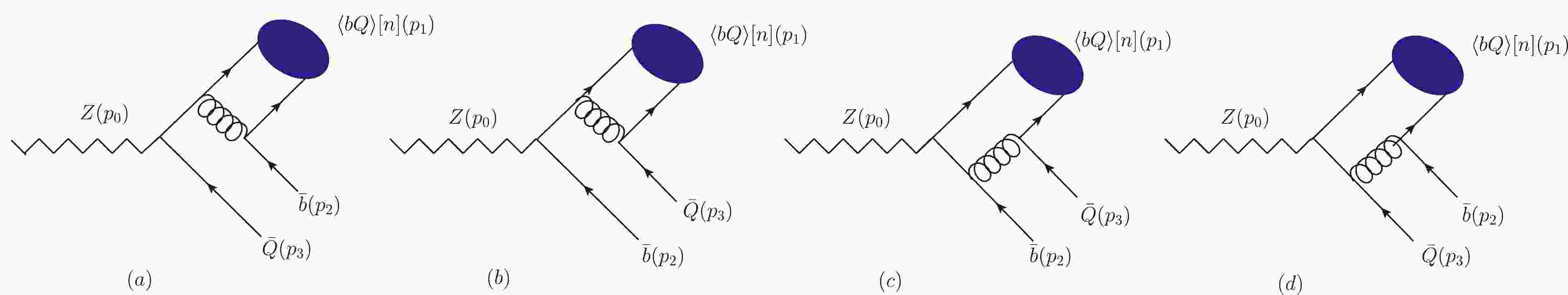
The diagrams for the process $Z(p_0) \to \langle bQ\rangle[n](p_1) + \bar b(p_2)+\bar Q(p_3)$ at tree level are shown in Fig. 1, where the heavy quark taken as $ Q = c $ and b represents $ \Xi_{bc} $ and $ \Xi_{bb} $, respectively. We can obtain the differential decay width of the process $Z (p_0) \to \langle bQ\rangle[n]({p_1}) + \bar b(p_2)+ \bar Q(p_3)$ using the NRQCD factorization approach [55, 56],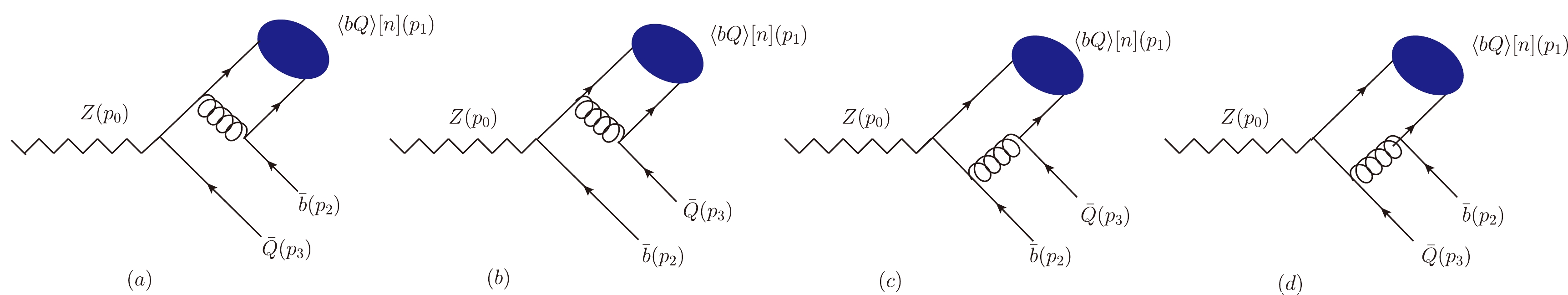

Figure 1.  (color online) Diagrams for $ Z \to \langle bQ\rangle [n] +\bar b+\bar Q $ at the leading order, where the heavy quark $ Q = c $ and b represents $ \Xi_{bc} $ and $ \Xi_{bb} $, respectively.

Here, the long-distance matrix element $ \langle {{\mathcal O^H}(n)}\rangle $ describes the hadronization of the diquark state $ \langle bQ\rangle[n] $ into the doubly heavy baryon $ \Xi_{bQ} $. Generally, $ \langle {{\mathcal O^H}(n)}\rangle $ can be approximately obtained from the original value of the Schrödinger wave function or its derivative. In this paper, we take $ \langle {{\mathcal O^H}(n)}\rangle = (|\Psi_{bQ}(0)|, |\Psi^{\prime}_{bQ}(0)|) $ for the S-wave and P-wave, which are derived from experimental data and non-perturbative theoretical methods, for example, the potential model, lattice QCD, and QCD sum rules [56–58].

The differential decay width ${\rm d}\hat\Gamma(Z \to \langle bQ\rangle[n] +\bar b+\bar Q)$ can be written as

where $ m_z $ and $ |M[n]| $ are the Z-boson mass and hard amplitude, respectively. The constant $ 1/3 $ arises from the spin average of the initial Z-boson, and the symbol "$ \sum $" represents the sum of color and spin for all final particles. The three-body phase space ${\rm d}\Phi_3$ with a massive quark or antiquark in the final state can be written as

The calculation for the three-body phase space has been discussed in Refs. [59, 60]. Then, Eq. (2) can be rewritten as

with $ s_{ij} = (p_i + p_j)^2 $. After using charge parity $C= -{\rm i}\gamma^2\gamma^0$, hard amplitude expressions $ M[n] $ for baryon production are obtained, which can also be easily gained from the familiar meson production [26, 39]. Here, we give brief descriptions. $C=-{\rm i}\gamma^2\gamma^0$ can be used to reverse one fermion line, which can be written as $ L_1= \bar u_{s_1}(k_{12}){\Gamma_{i+1}} S_F(q_i,m_i) \cdots S_F(q_1,m_1) \Gamma_1 v_{s_2}(k_2) $, where $ \Gamma_i $, $ S_F (q_i,m_i) $, $ s_{1,2} $, and $ i = (0, 1,...) $ are the interaction vertex, fermion propagator, spin index, and quantity of interaction vertices in the fermion line, respectively. According to charge parity, we have

If the fermion line does not include an axial vector vertex, we can readily obtain the expression

Otherwise, the amplitudes of baryon production can be obtained from familiar meson production, except with an additional $ (-1)^{(n+1)} $ coefficient for the pure vector case and a $ (-1)^{(n+2)} $ factor when including an axial vector case. In other words, the amplitude of $ Z\to \langle bQ\rangle[n]+\bar b+\bar Q $ can be written as

where $ M_i\; (i=1,~2,~3,~4) $ is the hard amplitude of familiar meson production, and $ M^a_i $ and $ M^v_i $ are the components of the axial vector amplitudes and pure vector amplitudes of $ M_i $, respectively.

Taking the traditional Feynman rules of Fig. 1 into considersion, we can obtain the amplitudes $ M_l[n] $ with $l=(a,b,c, d)$, which have the following expressions:

Here, $ \kappa=-C g_s^2 $, with color factor $ C_{ij,k} $. $ p_{11} $ and $ p_{12} $ are the momenta of the bottom quark and another heavy quark $ Q= (c,b) $ for $ \Xi_{bc} $ and $ \Xi_{bb} $ production. The vector and axial vector coupling constants of the $ Z_{Q\bar Q} $ vertex, that is, $ c_v^Q $ and $ c_a^Q $, have the following expressions:

Here, $ \theta_w $ is the Weinberg angle. With the help of Eq. (6) and inserting the spin projector $ \Pi_{p_1}^{[n]} $, the amplitude can be rewritten as

Here, the spin projector $ \Pi_{p_1}^{[n]} $ has the following form [61]:

where $ M_{bQ} \simeq m_b + m_Q $ is used to maintain gauge invariance.

Furthermore, the color factor $ C_{ij,k} $ can be easily obtained from Fig. 1, which has the following form:

Here, k, $a = (1, 2,\cdots,8)$, $ N = \sqrt {1/2} $, and $ i, j, m, n = (1, 2, 3) $ represent the diquark color indices, gluon color indices, normalization factor, and two outgoing antiquarks and two constituent quarks in the diquark color indices, respectively. For the $ \bar {\bf3}(\bf 6) $ state, the function $ G_{mnk} $ is identical to the antisymmetric function $ \varepsilon_{mjk} $ and symmetric function $ f_{mjk} $, which obey

For color $ \mathbf {\bar 3} $ and $ \mathbf 6 $ diquark state production, $ C_{ij,k}^2 = 4/3 $ and $ C_{ij,k}^2 = 2/3 $, respectively.

Meanwhile, diquark hadronization into a doubly heavy baryon is a non-perturbative procedure, which is factorized into a general coefficient $ \langle \mathcal O^H(n) \rangle $. This coefficient is connected to the wave function at the origin. In this paper, we take the usual assumption that the wave function of the color $ \bf\bar 3 $ state is equal to that of the color $ \bf 6 $ state, as discussed in Refs. [26, 39, 44, 45, 53]^①.

The transition probabilities of the color $ {\bf\bar3} $ and $ \bf 6 $ states are represented by $ h_{\bf\bar3} $ and $ h_{\bf6} $, respectively. Based on the NRQCD approach, a bound state of two heavy quarks with another light dynamical freedom of QCD $ \Xi_{bQ} $ can be described by a series of Fock states,

where v denotes the small relative velocity between heavy quarks in the rest frame of the diquark. For the color $ \bf\bar 3 $ state cases, one of the heavy quarks of the diquark can produce a gluon without altering its spin, which can divide into a light quark pair $ q\bar q $. Then, the diquark can capture a light quark q to construct a baryon. Regarding the color $ \bf 6 $ state, if the baryon is created by $ |(bQ)q\rangle $, the emitted gluon would alter the spin of the heavy quark, causing suppression of $ h_{\bf6} $. If the baryon is created from the $ |(bQ)qg\rangle $ parts, one of the heavy quarks produces a gluon without altering the spin of the heavy quark. Then, the gluon separates into $ q\bar q $. Additionally, a light quark q has the ability to produce gluons, which can be used to construct the component with $ qg $. These contributions are at the same level because a light quark may produce gluons easily, that is, $ c_1(v)\sim c_2(v)\sim c_3(v) $ [53]. We can then take the following approximation:

for the S-wave, and for P-wave,

To perform the numerical calculation, the following input parameters are taken: The $c,~b$-quark masses are $ m_c = 1.8\; {\rm GeV} $ and $ m_b = 5.1\; {\rm GeV} $, respectively. The Z-boson mass $ m_Z= $ 91.1876 GeV and the decay width $ \Gamma_Z = 2.4952\; {\rm GeV} $ are from the PDG [62]. For the values of $ |\Psi_{bc}(0)|^2 $ and $ |\Psi_{bb}(0)|^2 $, we adopt $ 0.065\; {\rm GeV^3} $ and $ 0.152\; {\rm GeV^3} $ [15], respectively. The masses of the $ \Xi_{bc} $ and $ \Xi_{bb} $ baryons are taken as $ m_{\Xi_{bc}}=6.9 \; {\rm GeV} $ and $m_{\Xi_{bb}}=10.2 \; {\rm GeV}$, respectively. The remaining input parameters are [62] $ G_F=1.1663787\times 10^{-5} $, which denotes the Fermi constant, and the Weinberg angle $ \theta_w={\rm arcsin}\sqrt {0.2312} $. The renormalization scale $ \mu_r $ is taken as $ 2m_c(2m_b) $ for the indirect production of $ \Xi_{bc}(\Xi_{bb}) $.

First, the decay widths of two main Z-boson decay channels for $ \Xi_{bQ} $ production are given in Table 1. From Table 1, we can see that the $ [^3S_1]_{\bar 3} $ state plays a leading role in the production of $ \Xi_{bb} $. The contribution from the $ [^3S_1]_{\bar 3} $ state can reach twice that from the $ [^1S_0]_6 $ state. As for $ \Xi_{bc} $ production, the situation is analogous to that of $ \Xi_{bb} $. Moreover, in the case of $ \Xi_{bc} $, the contribution from $ Z\to c\bar c $ is significantly smaller than that from $ Z\to b\bar b $, which is only a few percent.

$ \Gamma(Z\to Q\bar Q) $	$ \Xi_{bc} $					$ \Xi_{bb} $
	$ [^3S_1]_{\bar 3} $	$ [^3S_1]_6 $	$ [^1S_0]_{\bar 3} $	$ [^1S_0]_6 $		$ [^3S_1]_{\bar 3} $	$ [^1S_0]_6 $
$ Z\to c\bar c $	0.644	0.322	0.741	0.371		-	-
$ Z\to b\bar b $	33.01	16.51	24.14	12.07		1.999	1.028

Table 1.  Predicted decay widths $ \Gamma(Z\to Q\bar Q\to\Xi_{bc}(\Xi_{bb})+X) $ (unit: $ 10^{-6} $ GeV) with $ Q = (c,b) $ for the $ \Xi_{bc} $ and $ \Xi_{bb} $ baryons from each Z-boson decay channel.

To assess the doubly heavy baryon $ \Xi_{bQ} $ events generated at the LHC (CEPC), the corresponding branching ratio must be obtained from the Z-boson total decay width. At the LHC (CEPC), approximately $ 10^9(10^{12}) Z $-bosons can be produced per year [51, 63]. Based on the conditions mentioned above, the produced events of the double heavy baryon $ \Xi_{bc}(\Xi_{bb}) $ can be predicted at the LHC (CEPC). We list the total decay width, branching ratios, and events of the $ \Xi_{bc} $ and $ \Xi_{bb} $ baryons via Z-boson decay in Table 2, where contributions from each diquark state of the Z-boson decay channel are considered for the total decay width. From Table 2, we can reach the following conclusions:

	$ Z \to \Xi_{bc} $	$ Z\to \Xi_{bb} $
$ \Gamma({Z \to \Xi_{bQ}}) $	$ 89.71\times 10^{-6} $	$ 3.027\times 10^{-6} $
$ {\cal B}({Z \to \Xi_{bQ}}) $	$ 35.95\times 10^{ - 6} $	$ 1.213\times {10^{ - 6}} $
LHC events	$ 35.95 \times {10^3} $	$ 1.213 \times {10^3} $
CEPC events	$ 35.95 \times {10^6} $	$ 1.213 \times {10^6} $

Table 2.  Predicted total decay width (unit: GeV), branching fraction, and events of the $ \Xi_{bc} $ and $ \Xi_{bb} $ baryons in Z-boson decay.

● For the production of $ \Xi_{bb} $, the branching ratio $ {\cal B}(Z\to\Xi_{bb}+X) $ is approximately $ 10^{-6} $, which is comparable to the results given in Ref. [64].

● The branching ratio of $ {\cal B}(Z\to\Xi_{bc}+X) $ reaches $ 10^{-5} $ for the production of $ \Xi_{bc} $, which is also comparable to the predictions of $ {\cal B}(Z\to B_c+X) $ [65].

● At the CEPC, there are approximately $ 10^7 $-order $ \Xi_{bc} $ events and $ 10^{6} $-order $ \Xi_{bb} $ events obtained per year.

● In comparison, there are only approximately $ 10^4 $ order $ \Xi_{bc} $ events and $ 10^3 $ order $ \Xi_{bb} $ events produced at the LHC. However, the upgraded program of the HE(L)-LHC will significantly improve Z-boson yield events; thus, more $ \Xi_{bc} $ and $ \Xi_{bb} $ events will be produced.

● Considering the decay rate of the channels $ \Xi^+_{bc}\to \Xi^{++}_{cc}+X\simeq 7{\text%} $ [52], $ \Xi^{++}_{cc}\to \Lambda^+_c K^-\pi^+\pi^+\simeq 10{\text%} $ [66], and $ \Lambda^+_c\to pK^+\pi^+\simeq5{\text%} $ [67], approximately $ 10^4 $ reconstructed $ \Xi^+_{bc} $ events can be collected at the CEPC. These events are comparable to $ \Xi^{++(+)}_{cc} $ [47], which proves the observability of $ \Xi^{+}_{bc} $ via Z-boson decay.

Furthermore, the ratio of the $ \Xi^{+,0}_{bc} $ production rate $ {\cal R}(Z\to Q\bar Q\to\Xi_{bc}^{+,0}+X) $, which arises from Z-boson decay to $ \Lambda^+_c $ accompanied by $ K^-\pi^+\pi^+ $, has the following formula:

where X denotes all possible particles. First, we use the formula $ {\cal B}({Z\to Q\bar Q \to\Lambda^+_c})={\cal B}(Z\to Q\bar Q)\times f(Q\to\Lambda^+_c) $ to obtain $ \Gamma(Z\to Q\bar Q \to\Lambda^+_c) $. This is based on the total decay width, which can be directly related to the branching fraction. The branching fractions of $ Z\to Q\bar Q $ are taken from the PDG, that is, $ {\cal B}(Z\to c\bar c)=0.12 $ and $ {\cal B}(Z\to b\bar b)=0.15 $ [68]. The fragmentation fractions of a heavy quark to a particular charmed hadron are $ f(c\to\Lambda^+_c)=0.057 $ and $ f(b\to\Lambda^+_c)= $ 0.073 [69]. Then, we have

Second, according to the decay chains of $\Xi^{+,(0)}_{bc}\to \Xi^{++}_{cc}+X\simeq 7\%(1.5{\text%})$ [52], $\Xi^{++}_{cc}\to \Lambda^+_c K^-\pi^+\pi^+\simeq 10{\text%}$ [66], and $\Lambda^+_c\to pK^+\pi^+\simeq 5{\text%}$ [67], we can get the final results shown in Fig. 2. Here, the renormalization scale $ \mu_r $ is set to $ 2m_c $. $ {\cal R}(Z\to b\bar b\to\Xi^{+,0}_{bc}+X) $ is one magnitude larger than $ {\cal R}(Z\to c\bar c\to\Xi^{+,0}_{bc}+X) $, which indicates that the decay channel $ Z\to b\bar b $ provides key contributions compared with the $ Z\to c\bar c $ channel for indirect $ \Xi^{+,0}_{bc} $ production. Comparing the predictions of $ \Xi_{bc} $ in this study with $ \Xi_{cc} $ from our previous work [47] for Z-boson decay, there is a large gap between $ {\cal R}(Z\to c\bar c\to \Xi^{+,++}_{cc}+X) $ and $ {\cal R}(Z\to b\bar b\to \Xi^{+,0}_{bc}+X) $ of approximately one magnitude. This discrepancy indicates that it will be difficult to collect $ \Xi^{+,0}_{bc} $ in experiment collaborations. Moreover, our predictions for $ {\cal R}(Z\to Q\bar Q\to \Xi^0_{bc}+X) $ via the $ \Xi^{++}_{cc} $ channel reach the order of$ 10^{-5} $ in Z-boson decay, which is larger than those for the $ \Lambda^+_c\pi^- $ channel (of the $ 10^{-6} $ order) [70]. Thus, the observation of $ \Xi^0_{bc} $ via the $ \Xi^0_{bc}\to\Xi^{++}_{cc}+X $ channel is more feasible than that via the $ \Xi^0_{bc}\to\Lambda^+_c\pi^- $ channel.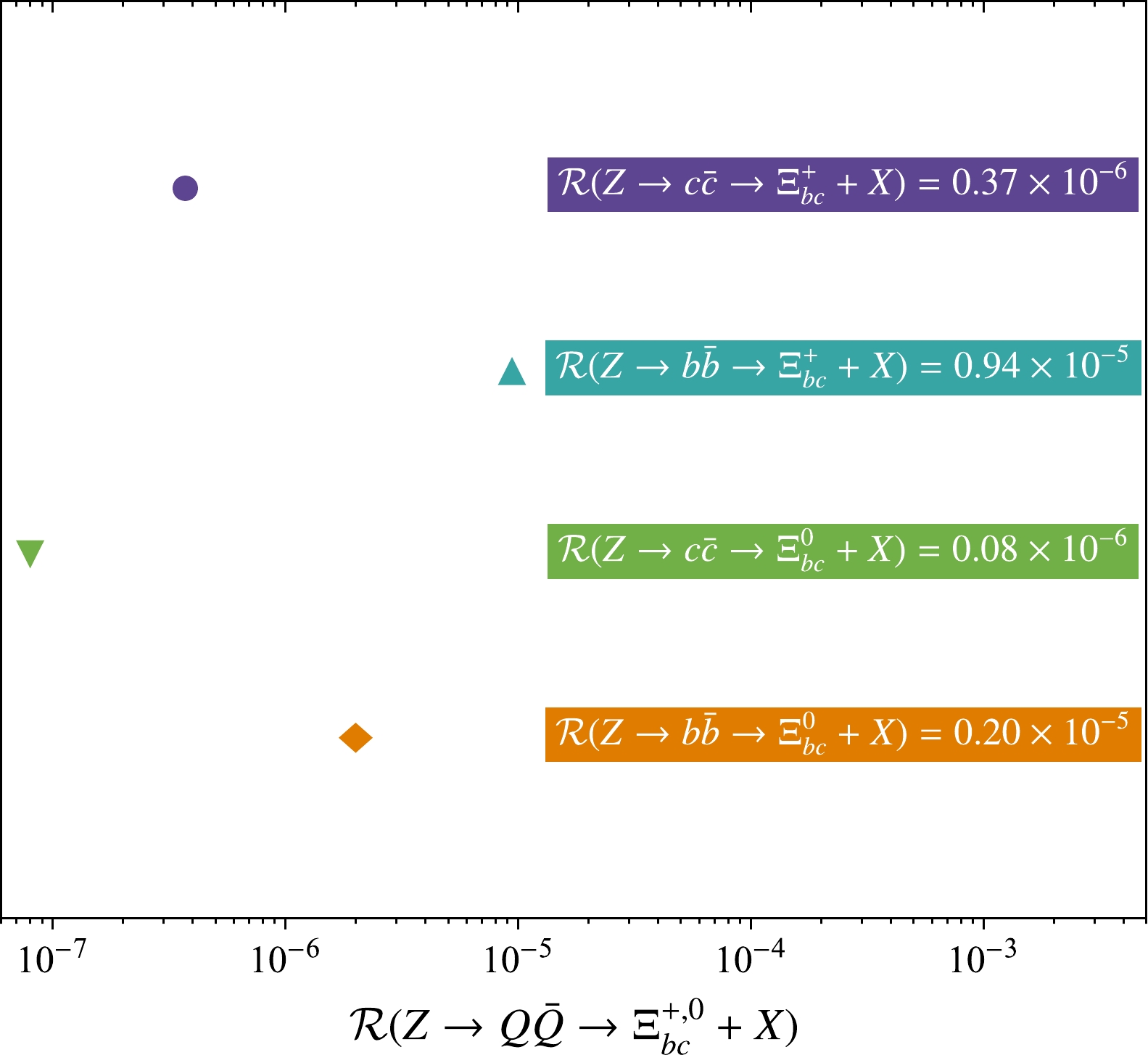

Figure 2.  (color online) Predictions for $ {\cal R}(Z\to Q\bar Q \to \Xi_{bc}^{+,0}+X) $ with four different Z-boson decay channels, where $ Q=(c,b) $. Here, the renormalization scale is set near $ \mu_r = 2m_c $.

To further study the production of $ \Xi_{bQ} $ via these considered decay channels and provide a reference for experimental research, we present the differential decay widths of $ \Xi_{bQ} $ with respect to the invariant mass $ s_{23} $ and energy fraction z in Figs. 3 and 4, where $ s_{i j} = (p_i + p_j)^2 $, and$ z = 2E_1/E_Z $, using the $ \Xi_{bQ} $ energy $ E_1 $ and Z-boson energy $ E_Z $.

Figure 3.  (color online) Invariant mass differential decay widths ${\rm d}\Gamma/{\rm d}s_{23}$ for the process $ Z \to \Xi_{bc}(\Xi_{bb})+X $ under the NRQCD factorization approach, where $ \mathbf{\bar 3(6)} $ indicates that the color quantum number is $ \bar {\mathbf 3}(\mathbf 6) $ of the diquark state, and "Total" denotes the total decay widths, which means that each diquark state has been summed.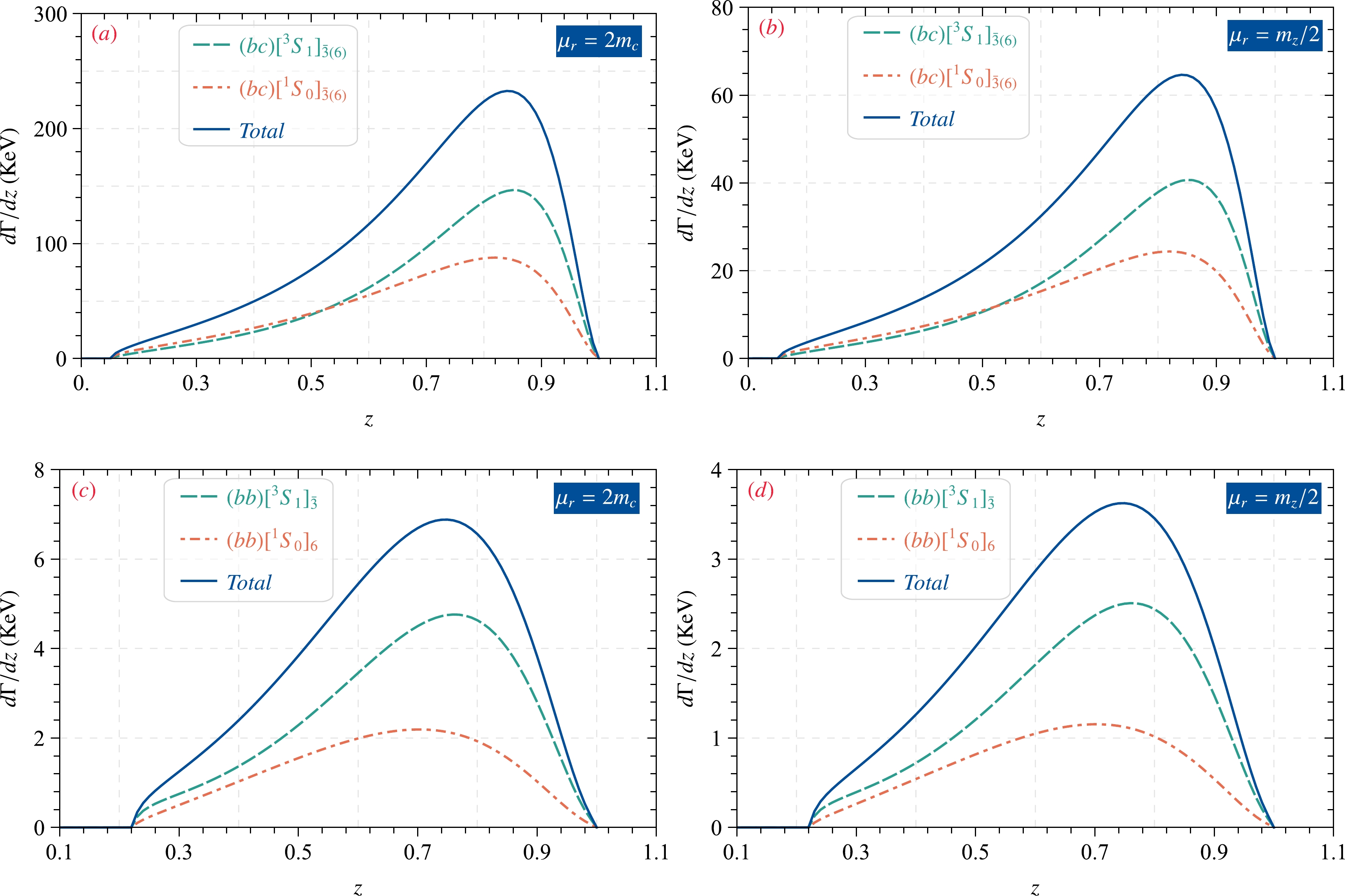

Figure 4.  (color online) Differential decay widths ${\rm d}\Gamma/{\rm d}z$ for the process $ Z \to \Xi_{bc}(\Xi_{bb})+X $ under the NRQCD factorization approach, where $ \mathbf{\bar 3(6)} $ indicates that the color quantum number is $ \bar {\mathbf 3}(\mathbf 6) $ of the diquark state, and "Total" denotes the total decay widths, which means that each diquark state has been summed.

● In Fig. 3, we find that the $ [^3S_1] $ state plays the leading role in the cases of $ \Xi_{bc} $ and $ \Xi_{bb} $ production. The curves ${\rm d}\Gamma/{\rm d}s_{23}$ have a similar behavior, which increase initially and then decrease with $ s_{23} $, with the peak located in the small region of $ s_{23} $.

● As shown in Fig. 4, the behavior of the differential decay widths changes with the energy fraction z-distribution, that is, ${\rm d}\Gamma/{\rm d}z$ is similar to ${\rm d}\Gamma/{\rm d}s_{23}$, which increases initially and then decreases. In the case of $ \Xi_{bb} $ production, the peak of ${\rm d}\Gamma/{\rm d}z|_{(bb)[^3S_1]_{\bar3}}$ is approximately $ z = 0.75 $, and ${\rm d}\Gamma/{\rm d}z|_{(bb)[^1S_0]_6}$ peaks near $ z = 0.7 $. As for $ \Xi_{bc} $, the peak of ${\rm d}\Gamma/{\rm d}z|_{(bc)[^3S_1]_{\bar 3(6)}}$ is approximately $ z = 0.8 $, and ${\rm d}\Gamma/{\rm d}z|_{(bc)[^1S_0]_{\bar 3(6)}}$ peaks near $ z = 0.85 $. Owing to the dominant effect of the quark fragmentation mechanism, the peaks of the differential decay widths for $ Z\to \Xi_{bc(bb)}+X $ with energy distribution are located in the larger z-region.

Finally, to discuss the theoretical uncertainties for the process $ Z\to\Xi_{bQ}+X $ precisely, $c,~b$-quark masses of $ m_c = 1.80 \pm 0.5\; {\rm GeV} $ and $ m_b = 5.1 \pm 0.5\; {\rm GeV} $, and the renormalization scale $ \mu_r = 2m_c(m_z/2) $ for $ \Xi_{bc} $ and $ \mu_r=2m_b(m_z/2) $ for $ \Xi_{bb} $ can be considered. Here, the uncertainties from $ |\Psi_{bQ}(0)|^2 $ are not discussed; they are an overall coefficient in calculations and can be computed out easily. The total decay widths within uncertainties arising from the above input parameters are presented in Table 3, which shows that

$ \mu_r $	$ m_Q $	$ \Xi_{bc} $					$ \Xi_{bb} $
		$ [^3S_1]_{\bar 3} $	$ [^3S_1]_6 $	$ [^1S_0]_{\bar 3} $	$ [^1S_0]_6 $		$ [^3S_1]_{\bar 3} $	$ [^1S_0]_6 $
	$ m_c = 1.30 {\rm GeV} $	100.4	50.19	67.07	33.53		1.999	1.028
$ 2m_c $	$ m_c = 1.80 {\rm GeV} $	34.40	17.20	25.41	12.71		1.999	1.028
	$ m_c = 2.30 {\rm GeV} $	15.64	7.820	12.46	6.231		1.999	1.028
	$ m_c = 1.30 {\rm GeV} $	27.88	13.94	18.62	9.312		1.053	0.542
$ m_Z/2 $	$ m_c = 1.80 {\rm GeV} $	9.552	4.776	7.057	3.528		1.053	0.542
	$ m_c = 2.30 {\rm GeV} $	4.343	2.172	3.460	1.730		1.053	0.542
	$ m_b = 4.60 {\rm GeV} $	33.89	16.95	25.91	12.96		3.044	1.385
$ 2m_c $	$ m_b = 5.10 {\rm GeV} $	34.40	17.20	25.41	12.71		1.999	1.028
	$ m_b = 5.60 {\rm GeV} $	34.92	17.46	25.00	12.50		1.345	0.697
	$ m_b = 4.60 {\rm GeV} $	9.412	4.706	7.196	3.598		1.515	0.773
$ m_Z/2 $	$ m_b = 5.10 {\rm GeV} $	9.552	4.776	7.057	3.528		1.053	0.542
	$ m_b = 5.60 {\rm GeV} $	9.696	4.848	6.943	3.471		0.750	0.389

Table 3.  Decay width Γ (unit:$ 10^{-6} $) of the process $ Z\to\Xi_{bc}(\Xi_{bb})+X $ within theoretical uncertainties through changing the mass of the charm quark $ m_c = 1.80 \pm 0.5\; {\rm GeV} $ and the mass of the bottom quark $ m_b = 5.10\pm 0.5 \; {\rm GeV} $.

● For indirect $ \Xi_{bc} $ production in Z-boson decay, the decay width decreases as the c-quark mass increases, which is mainly ascribed to the suppression of phase space.

● Owing to the effect of the projector in Eq. (11), an abnormal phenomenon occurs in which the decay width increases as the b-quark mass increases for the $ \langle bc\rangle[^3S_1] $ state in indirect production via Z-boson decay. The $ Z\to \langle bc\rangle[^1S_0]+X $ decay width decreases as the b-quark mass increases. Moreover, the uncertainty caused by $ m_c $ is larger than that of $ m_b $.

● For the process $ Z\to\Xi_{bb}+X $ with the $ [^3S_1]_{\bar 3} $ and $ [^1S_0]_{6} $ cases, the decay width decreases as the b-quark mass increases.

In this study, we discuss in detail the indirect production of $ \Xi_{bc} $ and $ \Xi_{bb} $ via Z-boson decay based on the framework of NRQCD. After considering the contributions from the intermediate diquark states, that is, $ \langle {bc} \rangle [^3 S_1] _{\bar 3/6} $, $ \langle {bc} \rangle[^1 S_0]_{\bar 3/6} $, $ \langle {bb} \rangle[^1 S_0]_6 $, and $ \langle {bb} \rangle[^3 S_1]_{\bar 3} $, the branching ratio $ {\cal B}(Z\to\Xi_{bc}+X) $ is approximately of the order of $ 10^{-5} $, and $ {\cal B}(Z\to\Xi_{bb}+X) $ is of the $ 10^{-6} $ order. There will be $ 10^4(10^7) \Xi_{bc} $ events and $ 10^3(10^6) \Xi_{bb} $ events produced at the LHC (CEPC). Then, the change in the differential decay widths of $ \Xi_{bc} $ and $ \Xi_{bb} $ with $ s_{23} $ and z distributions is presented. Moreover, we estimate the production ratio $ {\cal R}(Z\to\Xi^{+,0}_{bc}+X) $ of $ \Xi^{+,0}_{bc} $ to $ \Lambda^+_c $ via the Z-boson decay channel $ c\bar c $ and $ b\bar b $ for the first time, resulting in values of up to $ 10^{-6} $ for the $ c\bar c $ channel and $ 10^{-5} $ for the $ b\bar b $ channel. Abundant $ \Xi_{bQ} $ baryon events and the considerable branching ratio $ \mathcal B(Z\to \Xi_{bQ}+X) $ demonstrate the observability of the $ \Xi_{bQ} $ baryon in Z-boson decay during the experiment. Thus, we believe that it is worthwhile and feasible to search for the $ \Xi_{bQ} $ baryon through Z-boson decay at the LHC and CEPC.

In conclusion, at present, studies on the decay properties of doubly heavy baryons are discussed via their decay models. Especially in LHCb collaboration reports [71, 72] and theoretical results from Qin [52], decay models and their observational possibilities have been discussed. Inspired by the observation of the doubly-charmed baryon $ \Xi_{cc}^{++} $, the $ \Xi_{bc} $ baryon may be detected by the decay channels $ \Xi_{bc}\to\Xi_{cc}^{++}(\to p K^-\pi^+\pi^+)+X $, where X represents all possible particles. The advantage of this approach in detecting $ \Xi_{bc} $ is that the detection efficiency will be greatly improved because only $ \Xi_{cc}^{++} $ needs to be reconstructed, as discussed in Ref. [52]. Similar to the $ \Xi_{bc} $ baryon, $ \Xi_{bb} $ may also be observed via $ \Xi_{bb}\to \Xi_{bc}(\to\Xi_{cc})+X $.

We are grateful for Professor Zhan Sun's valuable comments and suggestions.