Primordial black holes and third order scalar induced gravitational waves

Inflation theory predicts that cosmological perturbations originate from quantum fluctuations during inflation, which suggests that valuable information about the early Universe is encoded in these perturbations. On large scales ($ \gtrsim $1 Mpc), primordial curvature perturbations have been determined through observations of the cosmic microwave background (CMB) and large scale structures [1, 2], indicating a nearly scale-invariant power spectrum for primordial curvature perturbations with amplitudes of $ \sim 2\times 10^{-9} $. On small scales ($ \lesssim $1 Mpc), the constraints on primordial curvature perturbations are significantly weaker than those on large scales [3].

Over the past few years, primordial scalar perturbations with large amplitudes on small scales have attracted considerable interest because of their rich and profound phenomenology. If the amplitude of small-scale primordial curvature perturbations are sufficiently large, large-amplitude perturbation modes that enter the Hubble radius during the radiation-dominated (RD) era can lead to the production of primordial black holes (PBHs) [4–25], which are a reasonable candidate for the entire or an appreciable portion of dark matter (DM). Moreover, the process in which PBHs are formed is inevitably accompanied by scalar induced gravitational waves (SIGWs) [26–29].

SIGWs have been studied for many years [30]. The energy density spectra of SIGWs include valuable information about PBHs [31–55] and primordial non-Gaussianity [56–63]. Furthermore, recent studies on SIGWs were also extended to include the gauge issue [64–75], dumping effect [76–78], epochs of the Universe [79–90], and modified gravity [91–93]. The relationship between SIGWs and PBH formation was first studied in Ref. [31] using a monochromatic primordial power spectrum. In previous studies, only second order SIGWs were considered. In Ref. [94], the authors partly considered the third order effects of SIGWs, which are directly induced by first order scalar perturbation. They found that the effects of the third-order correction led to an almost $ 20\% $ increase in the signal-to-noise ratio (SNR) for Laser Interferometer Space Antenna (LISA) observations. Their results indicate that higher order effects are not dispensable, and it is necessary to consider higher order SIGWs when small-scale primordial curvature perturbations are sufficiently large. In Ref. [95], we studied third order SIGWs during the RD era systematically. In addition to the source terms of the first order scalar perturbation, the source terms of three types of second order perturbations induced by the first order scalar perturbation were considered completely. We found that the third order gravitational waves sourced by the second order scalar perturbations dominated the energy density spectra of third order SIGWs. The direct contributions of the source term of the first order scalar perturbation, which were studied in Ref. [94], were negligible compared to the total energy density spectrum of third order SIGWs.

In this paper, we investigate primordial curvature perturbations and PBHs in terms of SIGWs. We find that the effects of third order SIGWs have significant observational implications for LISA.

The perturbed metric in Friedmann-Lemaitre-Robertson-Walker (FLRW) spacetime with the Newtonian gauge takes the form

where $ \phi^{(n)} $ and $ \psi^{(n)} $$ (n=1,2) $ are the n-order scalar perturbations, $ V^{(2)}_i $ is the second order vector perturbation, and $ h_{i j}^{(n)} (n=2,3) $ are the n-order tensor perturbations. In the RD era, the first order scalar perturbation is given by [28, 29]

where $ \zeta_{\mathbf{k}} $ is the primordial curvature perturbations. The transfer function $ T_\phi(k \eta) $ in the RD era is

where we define $ x\equiv k\eta $. We simplify the higher order cosmological perturbations in terms of the $\mathrm{xPand}$ package [96] and obtain the equation of motion for third order SIGWs,

where $ \Lambda_{i j}^{l m}=\mathcal{T}_{i}^{l} \mathcal{T}_{j}^{m}-\dfrac{1}{2} \mathcal{T}_{i j} \mathcal{T}^{l m} $ is the transverse and traceless operator [69, 95], and $ \mathcal{T}_{i}^{l} $ is defined as $\mathcal{T}_{i}^{l}=\delta_{i}^{l}- \partial^{l} \Delta^{-1} \partial_{i}$. For the RD era, the conformal Hubble parameter $ \mathcal{H}=a'/a=1/\eta $. The source term $ \mathcal{S}^{(3)}_{l m} $ takes the form

where $ S_{lm,1}^{(3)} $, $ S_{lm,2}^{(3)} $, $ S_{lm,3}^{(3)} $, and $ S_{lm,4}^{(3)} $ are the source terms of first order scalar perturbation, second order tensor perturbation, second order vector perturbation, and second order scalar perturbation, respectively. The explicit expressions of these source terms are given by

In Eq. (8), we use the symbol of the symmetric tensor $ T_{(lm)}\equiv\dfrac{1}{2}(T_{lm}+T_{ml}) $. Eq. (4) in momentum space can be solved using the Green’s function method, namely,

where we define $ h^{\lambda}_{\mathbf{k}}(\eta)=\varepsilon^{\lambda, ij}(\mathbf{k})h_{ij}^{(3)}(\mathbf{k}, \eta) $ and $ \mathcal{S}^{\lambda}_{\mathbf{k}}(\eta)= -\varepsilon^{\lambda, lm}(\mathbf{k})S_{lm}^{(3)}(\mathbf{k}, \eta) $, and $ \varepsilon_{i j}^{\lambda}(\mathbf{k}) $ is the polarization tensor, which satisfies $ \varepsilon_{i j}^{\lambda}(\mathbf{k}) \varepsilon^{\bar{\lambda}, ij}(\mathbf{k})\delta^{\lambda \bar{\lambda}}=2 $ and $\delta^{\lambda\bar{\lambda}}\varepsilon^{\bar{\lambda}, lm}(\mathbf{k})\varepsilon^{\bar{\lambda}}{ij}(\mathbf{k})= \Lambda_{i j}^{lm}(\mathbf{k})+A_{i j}^{lm}(\mathbf{k})$. Here, $ A_{i j}^{lm}(\mathbf{k}) $ is defined as [69]

where $ \left(\mathbf{k}_i/|k|,e_i,\bar{e}_i \right) $ is the normalized bases in three dimensional momentum space. Note that $ A_{i j}^{lm}(\mathbf{k}) $ is an antisymmetric tensor; therefore, $ A_{i j}^{lm}T_{lm}=A_{i j}^{lm}T^{ij}=0 $ for the arbitrary symmetric tensor $ T_{ij} $. In the calculations of the second and third order SIGWs, $ A_{i j}^{lm} $ only acts on the symmetric tensor. In this case, we obtain $ A_{i j}^{lm}=0 $ and $ \delta^{\lambda\bar{\lambda}}\varepsilon^{\bar{\lambda}, lm}(\mathbf{k})\varepsilon^{\bar{\lambda}}{ij}(\mathbf{k})=\Lambda_{i j}^{lm}(\mathbf{k}) $. There are four types of source terms in Eq. (4); it is convenient to divide $ h^{\lambda}_{\mathbf{k}}(\eta) $ into four parts $ h^{\lambda}_{\mathbf{k}}(\eta)=\sum_{i=1}^{4}h^{\lambda}_{\mathbf{k},i}(\eta) $. The formal expressions of $ h^{\lambda}_{\mathbf{k},i}(\eta) $ are

where $ I^{(3)}_i (i=1,2,3,4) $ are the kernel functions of the third order SIGWs, which take the form

Here, we define $ |\mathbf{k}-\mathbf{p}|=uk $, $ |\mathbf{k}-\mathbf{q}|=wk $, $ |\mathbf{p}-\mathbf{q}|=\bar{u}p= \bar{u}vk $, and $ q=\bar{v}p=\bar{v}vk $. $ f_{i}^{(3)}\left(u,\bar{u},\bar{v},\bar{x})\right) $ $ (i= $ 1, 2, 3, 4) are transfer functions of the four types of source terms in Eqs. (6)–(9), which are given in Appendix A. We consider a monochromatic primordial power spectrum

where $ k_* $ is the wavenumber at which the power spectrum has a δ-function peak. In the case of a monochromatic primordial power spectrum, the explicit expression of the energy density spectra of third order SIGWs in the RD era is given by [95]

where $ \mathcal{P}^{ij}_h $ is the power spectra of third order SIGWs,

where $ \tilde{k}=k/k_* $ is a dimensionless parameter. The explicit expressions of X, Y, and $ w_{\pm} $ are given in Appendix B. The details of the polynomials $ \mathbb{P}^{i j}_{a} $ can be found in Ref. [95]. Note that the energy density of the gravitational waves decays as radiation; hence, the current total energy density spectra of the SIGWs can be approximated using [97]

where $ \Omega^{(2)}_{\mathrm{GW}}(\eta, k) $ is the energy density spectrum of second order SIGWs, which has been studied systematically in previous studies [29, 98].

The monochromatic primordial power spectrum corresponds to monochromatic PBH formation. The possibility of forming a PBH can be calculated in terms of the amplitude of the primordial power spectrum [7, 36],

where $ \sigma^2 \equiv\langle\zeta^2\rangle=\int \mathcal{P}_\zeta(k) \mathrm{d} \ln k=A_{\zeta} $ is the variance of primordial curvature perturbation, and $ \zeta_c \simeq 1 $ is the threshold value to form a PBH [94, 99–101]. Moreover, the mass of the PBH can be approximated using the frequency of the δ-function peak,

where $ f_*=k_*/(2\pi) $, and $ g_*^{\text {form }} $ is the effective degrees of freedom when PBHs are formed. Then, the fraction of PBHs can be evaluated in terms of β and $ m_{\mathrm{pbh}} $

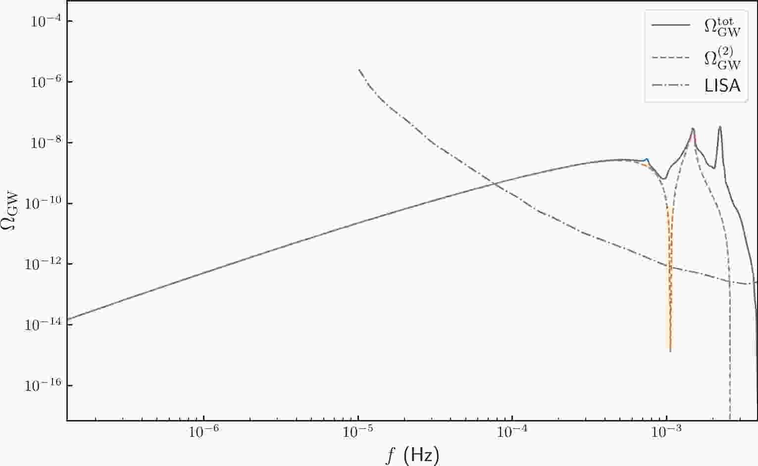
In the case of monochromatic PBH formation, Eqs. (21)–(23) show that β and $ m_{\mathrm{pbh}} $ are determined by the amplitude of the primordial power spectrum $ A_{\zeta} $ and the frequency of the δ-function peak $ f_* $, respectively. Furthermore, the fraction of PBHs $ f_{\mathrm{pbh}} $ increases with $ k_* $ and $ A_{\zeta} $. This strong correlation between PBHs and the concomitant SIGWs signals may offer a promising approach to detecting PBHs in upcoming gravitational wave experiments, such as LISA. Figure 1 shows the energy density spectra of SIGWs compared with the sensitivity curves of LISA. We find that the effects of third order SIGWs extend the cutoff frequency from $ 2f_* $ to $ 3f_* $ and have significant observational implications for LISA.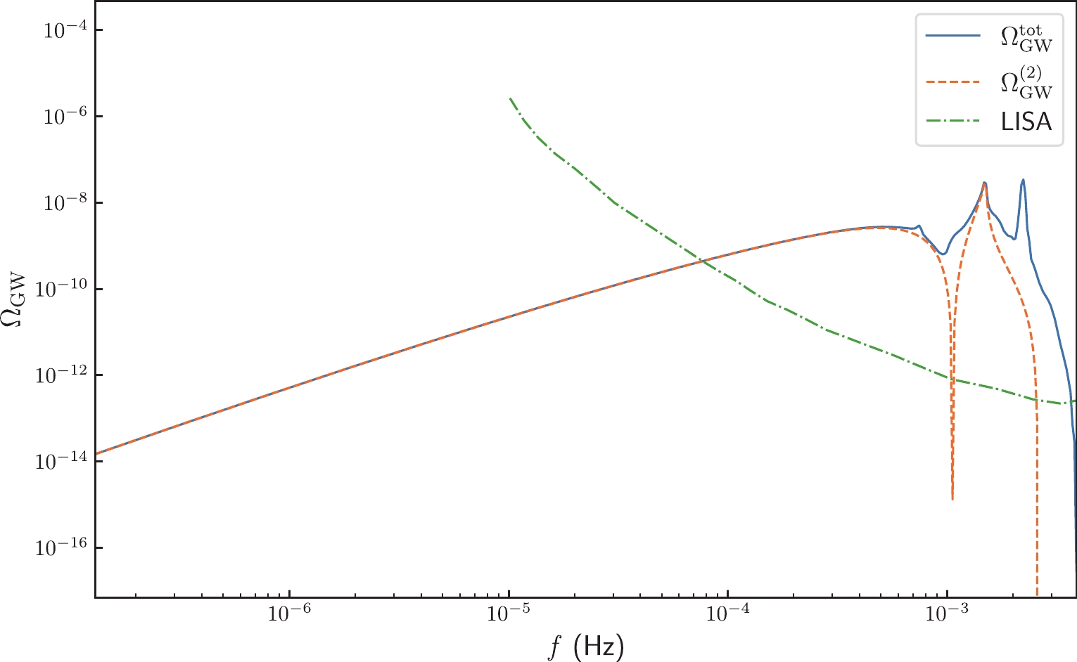

Figure 1.  (color online) Energy density spectra of SIGWs to the second order $\Omega^{(2)}_{\rm GW}$ (orange curve) and third order $\Omega^{\mathrm{tot}}_{\rm GW}= $$ \Omega^{(2)}_{\rm GW}+ \Omega^{(3)}_{\rm GW}$ (blue curve) as functions of frequency f. We set $ f_*=1.3\times 10^{-3} $Hz and $ A_{\zeta}=0.02 $.

To quantify the effects of third order SIGWs, we calculate the SNR ρ for LISA, which is given by [102–106]

where $ \Omega_n(f) = 2ı^2f^3S_n/3H_0^2 $, $ S_n $ is the strain noise power spectral density, and T is the observation time. Here, we set $ T=4 $ years. In Figs. 2 and 3, we plot the SNR curves obtained for the LISA experiment. More precisely, Fig. 2 shows the relationship between the SNR and $ m_{\mathrm{pbh}} $ for a given $ A_{\zeta} $, revealing that the effects of third order SIGWs lead to an approximately $ 200\% $ increase in the SNR for the frequency band from $ 1.6\times 10^{-3} $Hz to $ 10^{-5} $Hz, corresponding to PBHs with masses in the range $ 4\times 10^{-12}M_{\odot} \sim 10^{-7}M_{\odot} $. Figure 3 shows the relationship between the SNR and $ A_{\zeta} $ for a given $ m_{\mathrm{pbh}} $. The SNR and corresponding third order correction increase with the amplitude of the small-scale primordial power spectra $ A_{\zeta} $. Because the effects of third order SIGWs significantly affect the total energy density spectrum of the SIGWs, it is necessary to compare the energy density of the third order SIGWs $\rho_{\rm GW}^{(3)}$ with that of the second order SIGWs $\rho_{\rm GW}^{(2)}$. If we assume $\rho_{\rm GW}^{(3)} < \rho_{\rm GW}^{(2)}$, we will obtain a critical value $ A_* $ for the amplitude of the small-scale primordial power spectra. The critical value $ A_* $ can be calculated via

Figure 2.  (color online) SNR of LISA as a function of $ m_{\mathrm{pbh}} $ for $\Omega^{\mathrm{tot}}_{\rm GW}=\Omega^{(2)}_{\rm GW}+\Omega^{(3)}_{\rm GW}$ ($ \rho^\mathrm{tot}=\rho^{(2)}+\rho^{(3)} $, blue solid curve) and $ \Omega^{(2)}_{\rm GW} $ ($ \rho^{(2)} $, orange dashed curve). We set $ A_{\zeta}=0.02 $. We also give $\Delta \rho/\rho^{\rm tot} = \rho^\mathrm{tot}/\rho^{(2)}-1$ in the bottom panel.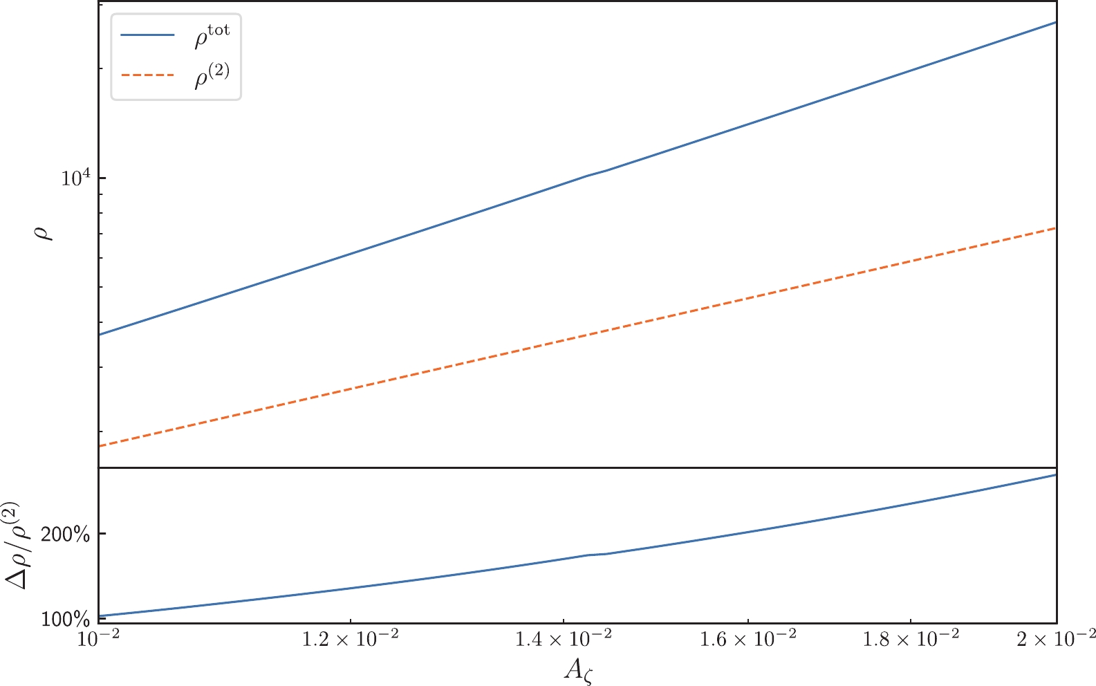

Figure 3.  (color online) SNR of LISA as a function of $ A_{\zeta} $ for $\Omega^{\mathrm{tot}}_{\rm GW}=\Omega^{(2)}_{\rm GW}+\Omega^{(3)}_{\rm GW}$ ($ \rho^\mathrm{tot}=\rho^{(2)}+\rho^{(3)} $, blue solid curve) and $\Omega^{(2)}_{\rm GW}$ ($ \rho^{(2)} $, orange dashed curve). We set $ f_*=1.3\times10^{-3} $. We also give $\Delta \rho/\rho^{\rm tot} = \rho^\mathrm{tot}/\rho^{(2)}-1$ in the bottom panel.

Solving Eq. (25), we obtain $ A_*=1.76\times 10^{-2} $. If $ A_{\zeta}>A_* $. Then, the energy density of third order SIGWs will be larger than that of second order SIGWs. Note that this critical value $ A_* $ is just an upper limit because $ \Omega^{(3)}_{\mathrm{GW}}(\eta, k) $ originates not only from $ \langle h^{(3)}_{\mathbf{k}} h^{(3)}_{\mathbf{k}'}\rangle $ but also$ \langle h^{(4)}_{\mathbf{k}} h^{(2)}_{\mathbf{k}'}\rangle $. The study of fourth order SIGWs is extremely difficult because all three types of third order perturbations must first be calculated. In this paper, we do not consider the effect of $ \langle h^{(4)}_{\mathbf{k}} h^{(2)}_{\mathbf{k}'}\rangle $. Predictably, this leads to a larger SNR and a smaller critical value $ A_* $.

In this paper, we study third order SIGWs and calculate the corresponding energy density spectrum. We find that the third order correction extends the cutoff frequency from $ 2f_* $ to $ 3f_* $. The relationships between the SNR of LISA and the monochromatic primordial power spectrum are studied systematically. For PBHs with masses in the range $ 4\times 10^{-12}M_{\odot} \sim 10^{-7}M_{\odot} $, the effects of third order SIGWs lead to an approximately $ 200\% $ increase in the SNR. For a given $ f_* $, the SNR and third order correction increase with $ A_{\zeta} $. We note that there is a critical value $ A_* $, such that when $ A_{\zeta}>A_* $, the energy density of third order SIGWs will be larger than that of second order SIGWs. We conclude that third order SIGWs are dominated by the source term of second order scalar perturbation $ \mathcal{S}^{(3)}_{4}\sim \phi^{(1)}\psi^{(2)} $. Third order SIGWs from a general primordial power spectrum are not considered here because of the difficulties in numerical calculation. A complete study of higher order SIGWs may be presented in future papers.

We thank Prof. S. Wang, Dr. Y.H. Yu, and Dr. J.P. Li for useful discussions. We also acknowledge the $\mathrm{xPand}$ package [96].

In this appendix, we briefly summarize the explicit expressions of $ f_{i}^{(3)}\left(u,\bar{u},\bar{v},\bar{x})\right) $$ (i=1,2,3,4) $ [95].