


 Abstract
 HTML
HTML Reference
 Related
 PDF
PDF


-
The atomic nucleus as a typical quantum many-body system exhibits many distinct properties or effects, such as shell effects and pairing correlations, which have attracted great interests in the past decades. The mass or equivalently the binding energy of a nucleus, as one of the most fundamental properties, can reflect many underlying physical effects, as can its derived quantities. So far, with the development of modern accelerator facilities, the masses for about 2500 nuclei have been measured [1]. However, there is still a large uncharted territory of atomic nuclei that cannot be measured or accessed experimentally in the foreseeable future.
Many theoretical efforts have been devoted to describing and predicting nuclear masses, which have achieved great success. For a recent review, see Ref. [2]. The first attempt to account for nuclear masses was the semi-empirical mass formula, which is commonly referred to as the Weizsäcker-Bethe mass formula [3–5]. Later, many different mass formulas within the macroscopic-microscopic framework have been developed and have already achieved a relatively high accuracy with respect to the available mass data, such as the finite-range droplet model [6, 7], the spherical-basis nuclear mass formula [8, 9], and the Weizsäcker-Skyrme model [10–12]. According to density functional theory, a series of Skyrme Hartree-Fock-Bogoliubov (HFB) mass models [13–16], as well as the Gogny HFB [17, 18] and relativistic mean field ones [19], have been constructed. Moreover, many microscopic mass-table-type calculations have been performed with either nonrelativistic [20–23] or relativistic [24–31] density functional theories.
Recently with the rapid development of artificial intelligence, many machine learning tools have been engaged in a variety of disciplines in science; nuclear physics is no exception [32–34]. Focusing on learning nuclear masses, the pioneering work was carried out in 1992: Gazula et al. used feedforward neural networks to learn the existing data on nuclear stability and mass excesses [35]. When the nuclear masses were learned directly, most of the obtained root-mean-square (rms) deviations with respect to the available experimental data were smaller than 2 MeV but larger than 0.5 MeV [35–42]. Very recently, by considering a physically motivated feature space and a soft physics constraint with Garvey-Kelson relations [43], the rms deviation was reduced to
$ \sigma_{\mathrm{rms}}=186 $ keV for the training set and 316 keV for the entire Atomic Mass Evaluation 2016 (AME2016) [44] with$ Z\geq 20 $ [45]. Additionally, the strategy that models the mass differences between theoretical and experimental values has been proposed, which makes the machine learning tools focus on the physical effects that cannot be described by theory and increases the accuracy of theoretical predictions. Up to now, with this strategy, many machine learning tools have been applied to learn and predict nuclear masses, such as feedforward neural networks [46, 47], Bayesian neural networks (BNNs) [48–54], the radial basis function (RBF) [52, 55–61], kernel ridge regression (KRR) [62−66], image reconstruction techniques [67] , trees and forests [68], the light gradient boosting machine [69], and the Bayesian probability classifier [70].Among these machine learning tools, the KRR is one of the powerful machine learning approaches, which extends ridge regression to the nonlinear case by learning a function in a reproduced kernel Hilbert space. The KRR approach was firstly introduced to improve nuclear mass predictions in 2020 [62]. It is found that the accuracy of the KRR approach in describing experimentally known nuclei is at the same level with other machine learning approaches, and has the advantage that it can avoid the risk of worsening the mass predictions for nuclei at large extrapolation. Later on, it was extended to include the odd-even effects (KRRoe) by remodulating the kernel function, which resulted in an accuracy of
$ \sigma_{\rm rms}=128 $ keV for nuclear mass predictions [63]. Recently, a multi-task learning framework for nuclear masses and separation energies was developed by introducing gradient kernel functions to the KRR approach, which improves the predictions of both nuclear masses and separation energies [64]. The successful applications of the KRR approach in nuclear masses [62–66] have stimulated other applications in nuclear physics, including the energy density functionals [71], charge radii [72], and neutron-capture cross-sections [73].Despite the successful application of machine learning to various physical problems, such as describing and predicting nuclear masses, physicists should not merely be satisfied with a solution for a certain problem but should also gain physical insights by exploiting artificial intelligence [74–76]. To achieve this, it seems that a better understanding of the abilities of the machine learning tools to capture the known physics will be beneficial. In nuclear physics, a feasible way to estimate these abilities is to learn the nuclear mass table, because nuclear mass as a fundamental property carries much known physics. Actually, by learning the experimental mass data, the ability of the machine learning tool to grasp essential regularities of nuclear physics has been addressed [35]. In this paper, we focus on the theoretical nuclear mass table, with the following two considerations: (1) Learning the theoretical nuclear mass table avoids the unknown physics, and it is relatively easy to quantify the physical effects in a theoretical model. (2) The number of theoretical data is not limited by facilities compared with experimental data, and the performance of the machine learning tools depends on the data number. With the help of theoretical mass models, the quality of the neural network extrapolation was examined in Ref. [41] and the capability of systematically describing nuclear ground-state energies was addressed in Ref. [77].
Among various theoretical nuclear mass tables, the mass table based on the relativistic continuum Hartree-Bogoliubov (RCHB) theory [29] is used in the present paper. Starting from the successful covariant density functional theory that includes the Lorentzian invariance from the very beginning [78–86] and employing the Bogoliubov transformation in the coordinate representation, the RCHB theory [87, 88] provides a unified and self-consistent treatment of continuum, mean-field potentials and pairing correlations [81]. As the first nuclear mass table including continuum effects, the RCHB mass table addressed the continuum effects crucial to drip-line locations and predicted 9035 bound nuclei with
$8\leqslant Z \leqslant 120$ , which extends the existing nuclear landscapes remarkably. Limited to the assumption of spherical symmetry, the rms deviation of the RCHB mass table with respect to the 2284 known nuclei is 7.96 MeV, which is significantly reduced to 2.16 MeV when focusing on the nuclei with either a neutron or proton magic number [29]. By including the deformation degree of freedom, the deformed relativistic continuum mass table is being constructed [30, 89, 90]. Nevertheless, thanks to the spherical symmetry, in this study, the RCHB mass table frees us from analysing the deformation effects as well as the couplings between deformation and other effects. It should be noted that by learning the residuals between the RCHB mass predictions and the experimental data with the RBF approach, it was found in Ref. [61] that the machine learning approach can describe the deformation effects neglected in the RCHB mass calculations and improves the description of the shell effect and the pairing effect.In this paper, the RCHB mass table is learned by means of the KRR and KRRoe methods. As a first attempt, the ability of the machine learning tool to grasp physics is studied by examining the shell effects, one-nucleon and two-nucleon separation energies, odd-even mass differences, and empirical proton-neutron interactions. The influences of hyperparameters in the KRR method on the learning ability are also discussed.
-
In the kernel ridge regression approach [62, 91, 92], the predicting function can be written as
$ f(\mathit{\boldsymbol{x}}_{j}) = \sum\limits_{i=1}^{m}K(\mathit{\boldsymbol{x}}_{j},\mathit{\boldsymbol{x}}_{i})\omega_{i}, $

(1) where
$ \mathit{\boldsymbol{x}}_{i}, \mathit{\boldsymbol{x}}_{j} $ are input variables, m represents the number of training data,$ K(\mathit{\boldsymbol{x}}_{j},\mathit{\boldsymbol{x}}_{i}) $ is the kernel function, and$ \omega_{i} $ is the corresponding weight that is determined by training. The kernel function$ K(\mathit{\boldsymbol{x}}_{j},\mathit{\boldsymbol{x}}_{i}) $ measures the similarity between data and plays a crucial role in prediction. There are many choices for the kernel function, such as linear kernels, polynomial kernels, and Gaussian kernels. The commonly used Gaussian kernel is written as$ \begin{array}{*{20}{l}} K(\mathit{\boldsymbol{x}}_{j},\mathit{\boldsymbol{x}}_{i}) = \mathrm{exp}\left[-\dfrac{\|\mathit{\boldsymbol{x}}_{j}-\mathit{\boldsymbol{x}}_{i}\|^{2}}{2\sigma^{2}}\right], \end{array} $

(2) where
$ \|\cdot\| $ denotes the Euclidean norm, and the hyperparameter$ \sigma > 0 $ , defines the length scale of the distance that the kernel affects.The weight
$ \mathit{\boldsymbol{\omega}}=(\omega_{1},\cdots,\omega_{m})^{T} $ is obtained by minimizing the loss function$ L(\mathit{\boldsymbol{\omega}}) = \sum\limits_{i=1}^{m}[f(\mathit{\boldsymbol{x}}_{i})-y(\mathit{\boldsymbol{x}}_{i})]^{2} + \lambda \mathit{\boldsymbol{\omega}}^{T}\mathit{\boldsymbol{K}}\mathit{\boldsymbol{\omega}}, $

(3) where
$ \mathit{\boldsymbol{K}}_{ij}=K(\mathit{\boldsymbol{x}}_{i},\mathit{\boldsymbol{x}}_{j}) $ is the kernel matrix. The first term is the variance between the KRR predictions$ f(\mathit{\boldsymbol{x}}_{i}) $ and the data$ y(\mathit{\boldsymbol{x}}_{i}) $ . The second term is a regularizer that reduces the risk of overfitting, and$ \lambda\geqslant 0 $ is a hyperparameter that determines the strength of the regularizer. By minimizing the loss function, one can obtain the weight as follows:$ \begin{array}{*{20}{l}} \mathit{\boldsymbol{\omega}} = \left(\mathit{\boldsymbol{K}}+\lambda \mathit{\boldsymbol{I}}\right)^{-1}\mathit{\boldsymbol{y}}, \end{array} $

(4) where
$ \mathit{\boldsymbol{I}} $ is the identity matrix.In predicting nuclear masses, the input variables are the proton and neutron numbers of the nucleus, i.e.,
$ \mathit{\boldsymbol{x}}=(Z,N) $ , and the output variable$ f(\mathit{\boldsymbol{x}}) $ is the prediction of nuclear mass. The corresponding Gaussian kernel function is [62]$ \begin{array}{*{20}{l}} K(\mathit{\boldsymbol{x}}_{j},\mathit{\boldsymbol{x}}_{i}) = \mathrm{exp}\left[-\dfrac{(Z_{j}-Z_{i})^{2}+(N_{j}-N_{i})^{2}}{2\sigma^{2}}\right]. \end{array} $

(5) Later, a remodulated kernel function was designed to include the odd-even effects [63]:
$ \begin{aligned}[b] K(\mathit{\boldsymbol{x}}_{j},\mathit{\boldsymbol{x}}_{i}) =& \mathrm{exp}\left[-\dfrac{(Z_{j}-Z_{i})^{2}+(N_{j}-N_{i})^{2}}{2\sigma^{2}}\right] \\&+ \frac{\lambda}{\lambda_{\mathrm{oe}}} \delta_{\mathrm{oe}}\mathrm{exp}\left[-\dfrac{(Z_{j}-Z_{i})^{2}+(N_{j}-N_{i})^{2}}{2\sigma_{\mathrm{oe}}^{2}}\right], \end{aligned} $

(6) where
$\sigma,~\lambda,~\sigma_{\mathrm{oe}}$ , and$ \lambda_{\mathrm{oe}} $ are hyperparameters to be determined, and$ \delta_{\mathrm{oe}}=1 $ only when$ (Z_{i},N_{i}) $ have the same parity with$ (Z_{j},N_{j}) $ ; otherwise,$ \delta_{\mathrm{oe}}=0 $ . The second term is the odd-even term, which was introduced to enhance the correlations between nuclei that have the same parity of proton and neutron numbers [63]. The hyperparameters$ \sigma_{\rm oe} $ and$ \lambda_{\rm oe} $ play similar roles of σ and λ but are related to the odd-even term. It should be noted that here the odd-even effects are included by remodulating the kernel function, which does not increase the number of the weight parameters. This is different from the ways to introduce odd-even effects by building and training additional networks in Ref. [58], or by adding additional inputs, as reported in Ref. [50]. -
In the present work, the binding energies obtained via the systematic RCHB calculations with density functional PC-PK1 [93] are used as the dataset, which contains 9035 bound nuclei with proton number
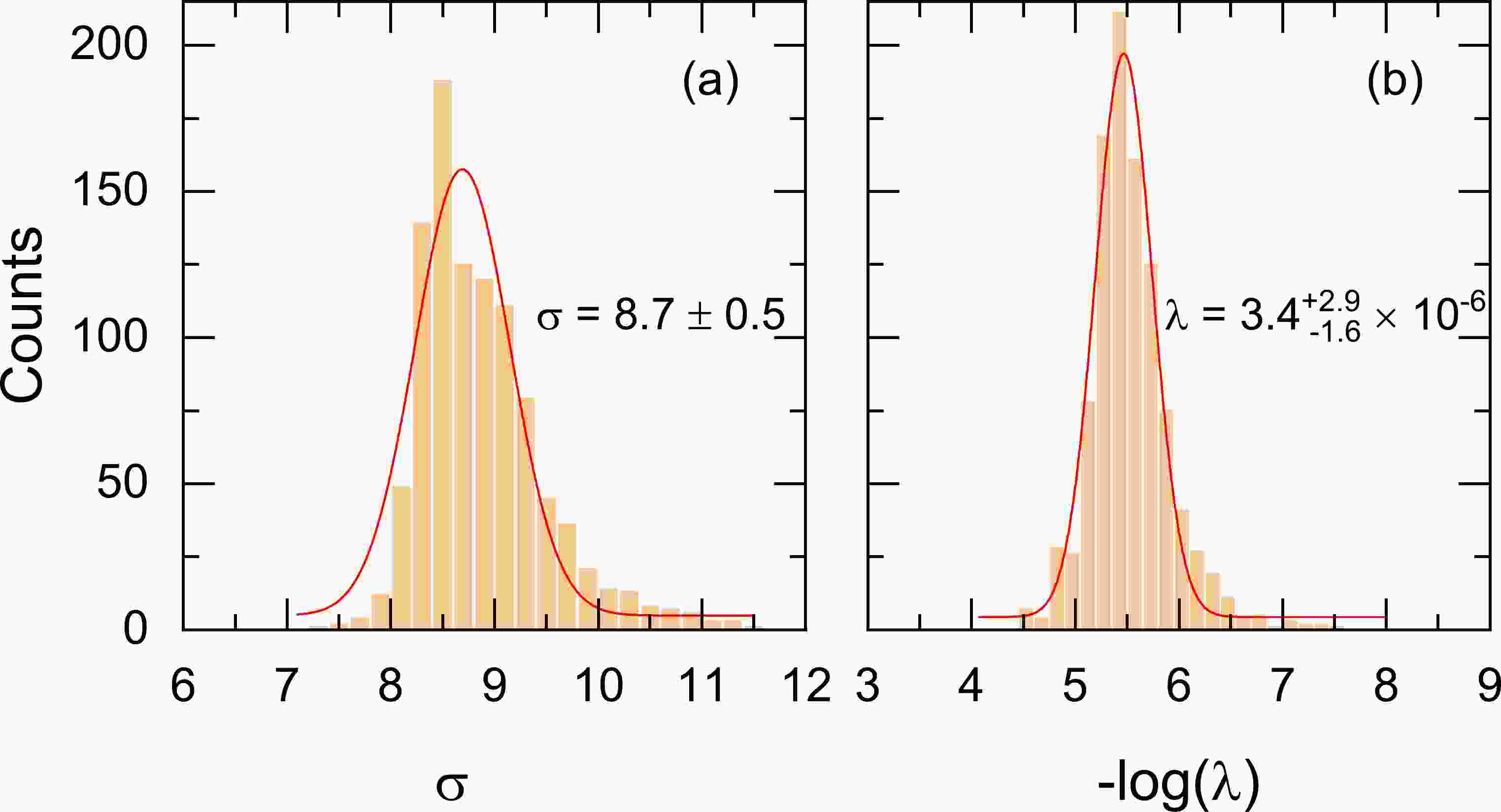
$ 8\leqslant Z \leqslant 120 $ [29]. Using a similar cross-validation procedure to Ref. [62] but with 1000 twofold cross-validations, the optimized hyperparameters of the KRR function are determined.Figure 1 shows the statistical distributions of the hyperparameters
$(\sigma,~\lambda)$ obtained from 1000 twofold cross-validations. Both σ and λ basically follow Gaussian distributions, and the center values of σ and λ, as well as their standard deviations, are obtained as$(8.7\pm 0.5 $ ,$ 3.4_{-1.6}^{+2.9}\times 10^{-6})$ . Compared with the hyperparameter$ \sigma=$ 2.38(17) determined in Ref. [62], the present hyperparameter σ is far larger. This may be because the present learning is based not on the mass residuals but directly on the binding energies, requiring a longer correlation distance.
Figure 1. (color online) Statistical distributions of the hyperparameters σ (left) and λ (right) for the twofold cross-validation on the 1000 sampled partitions. The center value and the standard deviation of Gaussian fitting are presented.
For the hyperparameters
$(\sigma,~ \lambda,~ \sigma_{\mathrm{oe}},~ \lambda_{\mathrm{oe}})$ in the KRRoe function, a search of optimized values in a 4-D parametric space needs lots of computing resources. Therefore, twofold cross-validation is performed only once, and the optimized hyperparameters are determined to be$ (2, 10^{-2}, 20, 10^{-7}) $ . -
With the optimized hyperparameters
$ (8.7,3.4\times10^{-6}) $ , the KRR approach with the Gaussian kernel is used to predict the nuclear binding energy of an arbitrary nucleus with the binding energies of all the other nuclei used for training, i.e., by means of the leave-one-out method. It is found that when the RCHB mass table is learned [29], the binding energies of 9035 nuclei obtained via the KRR predictions have an rms deviation of$ \sigma_{\mathrm{rms}}= $ 0.96 MeV with respect to the data in the RCHB mass table. This deviation is <1 MeV and is comparable to the typical values obtained by directly learning the experimental mass data with other machine learning methods such as feedforward neural networks [35–37, 39, 40, 77], a support vector machine [38], and mixture density networks [41, 45]. Thus, overall satisfactory performance of learning the RCHB mass table can be achieved via the KRR method with the Gaussian kernel. Similarly, with the optimized hyperparameters$ (2, 10^{-2}, 20, 10^{-7}) $ , the KRRoe approach is used to predict nuclear binding energies via the leave-one-out method. The corresponding rms deviation is$ \sigma_{\mathrm{rms}}=0.17 $ MeV, which marks a significant improvement on the KRR approach and is comparable to the accuracy of 0.13 MeV reported in Ref. [63]. In the following, several physical effects or derived quantities that embedded in nuclear binding energies, such as the shell effects, nucleon separation energies, odd-even mass differences and residual proton-neutron interactions, will be analysed based on the KRR (KRRoe) results and compared to the corresponding behaviors of the RCHB mass table, in order to evaluate the ability of the machine learning tool to grasp physics. -
As is well known, the shell effect is a quantum effect that plays an essential role in determining many properties of finite nuclear systems [94]. In the nuclear landscape, it is mostly reflected by the fact that a nucleus with some special proton numbers and/or neutron numbers, i.e., magic numbers, is far more stable than its neighboring nuclei. One reasonable way to quantitatively measure the shell effects over the nuclear landscape [94] is to examine the differences between nuclear masses and the values given by a phenomenological formula of the liquid drop model (LDM), such as the Bethe-Weizsäcker (BW) formula [3, 4], because the LDM regards an atomic nucleus as a classical liquid drop and does not include the shell effects. To this end, we first refit the BW formula to all 9035 data in the RCHB mass table and then analyse the shell effects by examining the mass differences between the BW formula and the RCHB mass table as well as the KRR predictions.
By fitting the 9035 data of the RCHB mass table, the five parameters of the BW formula are obtained, i.e., the volume coefficient
$a_{{V}}=13.64$ MeV, the surface coefficient$a_{{S}}=10.26$ MeV, the Coulomb coefficient$a_{{C}}=0.61$ MeV, the symmetry coefficient$a_{{A}}=19.78$ MeV, and the pairing coefficient$a_{{p}}=18.08$ MeV. In Fig. 2(a), the differences in the binding energies, i.e.,$E_{{b}}^{\mathrm{RCHB}}-E_{{b}}^{\mathrm{BW}}$ , between the RCHB mass table and the fitted BW formula are shown. The corresponding rms deviation$ \sigma_{\mathrm{rms}} $ is 10.18 MeV, which is about three times of the rms deviation 3.10 MeV obtained by fitting the BW formula to experimental data [2]. This results from the weakness of the BW formula for describing shell effects and nuclei away from the line of stability, whereas the RCHB mass table has larger shell effects and more nuclei away from the line of stability than the experimental data. In Fig. 2(a), some systematic differences in the features can be seen: (1) Comparing the nuclear regions near the magic numbers with those away from the magic numbers, it is shown that the deviations of the RCHB mass table from the fitted BW formula in the former regions are in general larger than the adjacent latter regions. This means the microscopic RCHB mass table gives more binding energies for nuclei with and close to magic numbers, which are the direct consequences of the shell effects. (2) In the relatively light$ A\leqslant 80 $ and considerably heavy$ A\geqslant 300 $ mass regions, the binding energies of the RCHB mass table are systematically lower than those of the fitted BW formula. (3) Near the neutron dripline regions, almost all the data in the RCHB mass table are more bound than the fitted BW formula. This is because the symmetry energy term$ -a_{A}(N-Z)^{2}/A $ in the BW formula plays a critical role in determining the binding energies of neutron-rich nuclei, whereas in the RCHB mass table, there are often many nuclei close to the neutron dripline having almost the same binding energies owing to considerations of pairing correlations and the continuum effect [29].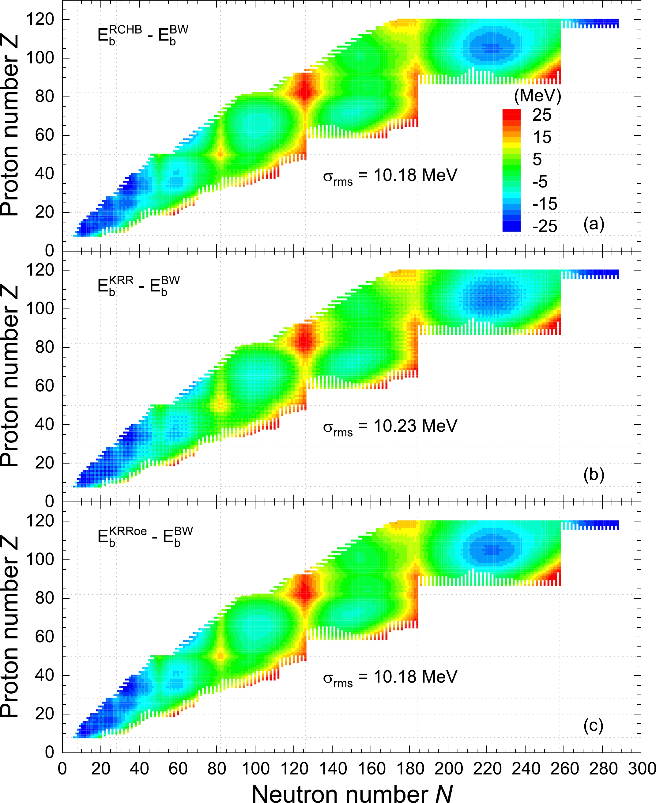
Figure 2. (color online) (a) Differences in the binding energies, i.e.,
$E_{{b}}^{\mathrm{RCHB}}-E_{{b}}^{\mathrm{BW}}$ , between the RCHB mass table [29] and the BW formula [3, 4] whose parameters are determined by fitting 9035 data from the RCHB mass table. The corresponding rms deviation$ \sigma_{\mathrm{rms}} $ is also given. The magic numbers are indicated by the vertical and horizontal dotted lines. (b, c) Same as (a) but for the KRR and KRRoe predictions.The differences in the binding energies of the RCHB, KRR, and KRRoe predictions with respect to the BW formula are shown in Fig. 2. Compared with Fig. 2(a), the three systematic features in Fig. 2(a) mentioned above are well reproduced in Fig. 2(b) and Fig. 2(c). In particular, the shell effects reflected in nuclear masses have been learned effectively by the KRR and KRRoe methods. It should be noted that although the KRR predictions catch the systematic features in Fig. 2(a), they lose some details in the differences; i.e., the differences between the RCHB mass table and the BW formula vary smoothly with respect to the nucleon number, whereas the differences between the KRR predictions and the BW formula exhibit grain structures. These details are better described by the KRRoe predictions, and no grain structure is seen in Fig. 2(c).
-
The nucleon separation energies, such as one- and two-nucleon separation energies, are first-order differential quantities of binding energies that can clearly show the shell effects. They also define the positions of nucleon drip lines. In this subsection, we compare the separation energies extracted from the KRR predictions with the optimized hyperparameters and those from the RCHB mass table.
The one-neutron separation energies, i.e.,
$S_{{n}}(Z,N)= E_{{b}}(Z,N)- E_{{b}}(Z,N-1)$ , extracted from the RCHB mass table and the KRR predictions are shown in Fig. 3(a) and Fig. 3(b), respectively. As summarized in Ref. [29] and shown in Fig. 3(a), the main features of$S_{{n}}$ from the RCHB mass table are as follows: (1) For a given isotopic (isotonic) chain,$S_{{n}}$ decreases (increases) with increasing neutron (proton) number; (2) Significant reductions in$S_{{n}}$ exist at the traditional magic numbers$N = 20,~28, ~50, ~82,~126$ as well as$ N=184 $ , indicating the shell closures; (3) because of the pairing correlations,$S_{{n}}$ has a ragged evolution pattern with the variation of the neutron number, which zigzags between even- and odd-A nuclei.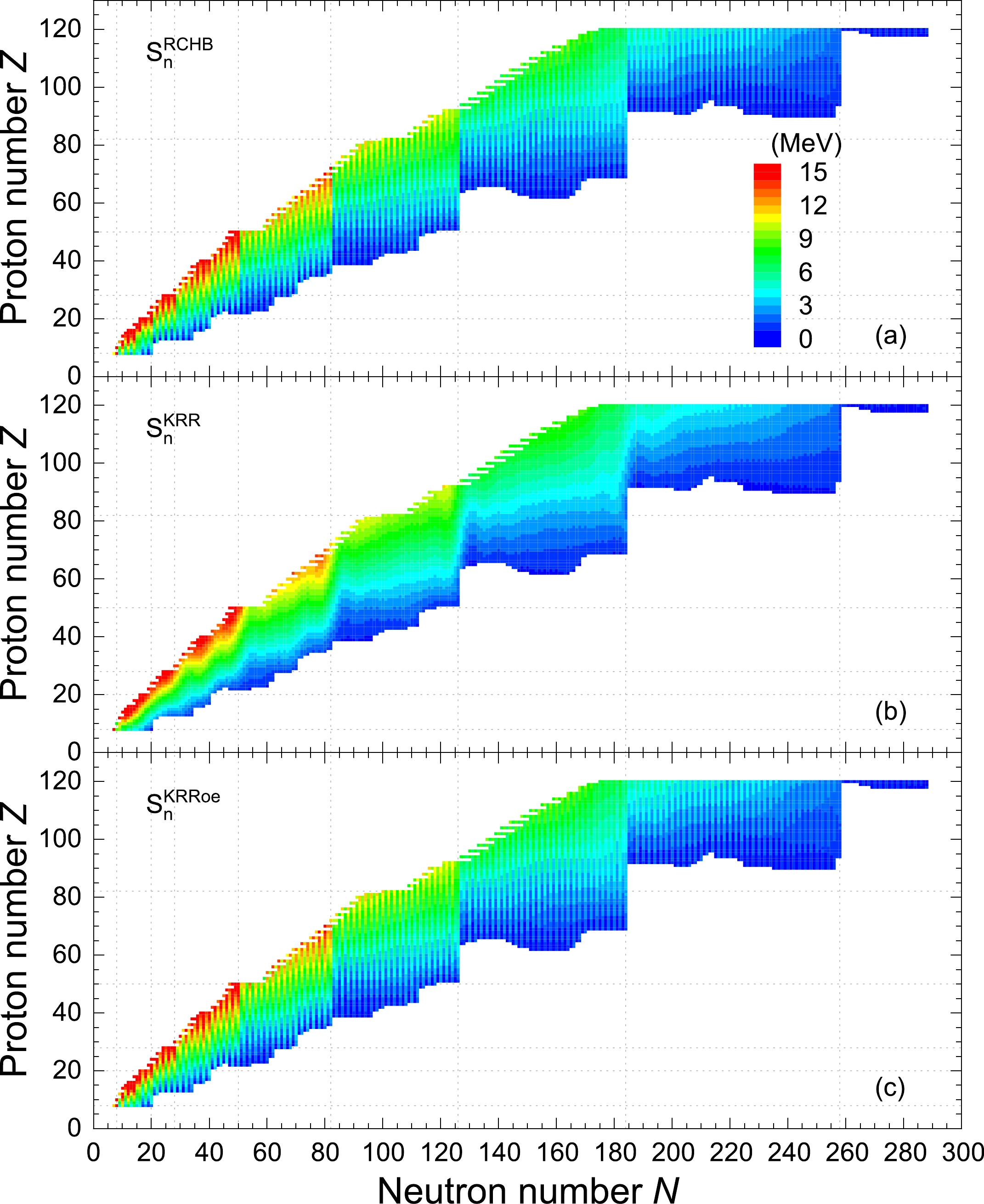
Figure 3. (color online) The one-neutron separation energies extracted from the RCHB mass table (a), in comparison with those from the KRR (b) and KRRoe (c) predictions. The values are scaled by colors.
As shown in Fig. 3(b) and Fig. 3(c), the
$S_{{n}}$ extracted from the KRR and KRRoe predictions also decreases (increases) with the increasing neutron (proton) number for a given isotopic (isotonic) chain, and there are drops at the traditional magic numbers$ N = 20, 28, 50, 82,126 $ as well as$ N=184 $ . However, in Fig. 3(b), these drops are not as sharp as those of the RCHB mass table. More obviously, the ragged evolution pattern in$S_{{n}}$ due to the pairing correlations is fully absent in the KRR results. For the KRRoe predictons in Fig. 3(c), owing to the explicit inclusion of the odd-even effects, the sharp drop at the magic number and the ragged evolution pattern are well reproduced.The two-neutron separation energies, i.e.,
$S_{{2n}}(Z,N)= E_{{b}}(Z,N)- E_{{b}}(Z,N-2)$ , extracted from the RCHB mass table and the KRR (KRRoe) predictions are shown in Fig. 4, where half of the$S_{{2n}}$ is scaled by colors in order to use the same scale as the one-neutron separation energies in Fig. 3. Similar to the$S_{{n}}$ , the$S_{{2n}}$ decreases (increases) with the increasing neutron (proton) number for a given isotopic (isotonic) chain, and there are significant drops at neutron shell closures. However, in contrast to the$S_{{n}}$ , the$S_{{2n}}$ does not show a ragged evolution pattern with the variation of neutron number, as the$S_{{2n}}$ is obtained by the difference between two nuclei with the same number parity. Furthermore, the nuclear landscape shown in Fig. 4 is slightly broader than that shown in Fig. 3 because of the differences between the two-neutron and one-neutron dripline nuclei.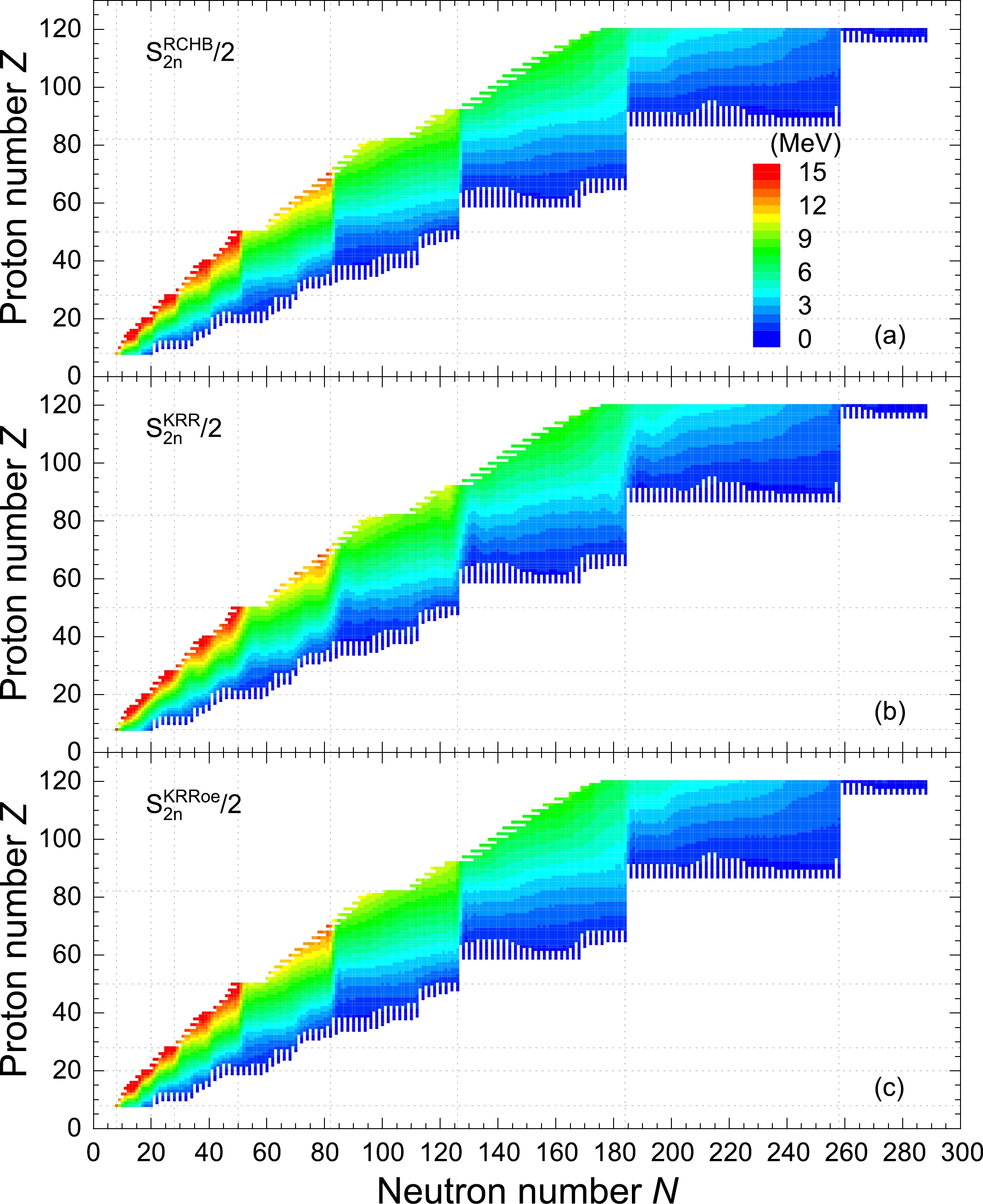
Figure 4. (color online) The two-neutron separation energies extracted from the RCHB mass table (a), in comparison with those from the KRR (b) and KRRoe (c) predictions. To have a better comparison with one-neutron separation energies in Fig. 3, here half of the two-neutron separation energies are shown and scaled by colors.
As shown in Fig. 4(b) and Fig. 4(c), the
$S_{{2n}}$ extracted from both the KRR and KRRoe predictions also decreases (increases) with the increasing neutron (proton) number for a given isotopic (isotonic) chain, and there are drops at neutron shell closures. Similar to the$S_{{n}}$ , the KRRoe method predicts these drops to be sharp, in accordance with the RCHB mass table but not the KRR method. Comparing Fig. 3 with Fig. 4, one can easily find that the learning performance of the$S_{{2n}}$ using the KRR function is better than that of the$S_{{n}}$ . Quantitatively, the rms deviation of the KRR predictions with respect to the RCHB mass table is 0.49 MeV for the$S_{{2n}}$ , compared with 1.12 MeV for the$S_{{n}}$ . For the KRRoe predictions, the corresponding rms deviations of$S_{{2n}}$ and$S_{{n}}$ are 0.18 and 0.24 MeV, respectively, both of which exhibit a significant improvement with respect to the KRR one.According to the analyses of the one- and two-neutron separation energies, one can conclude that although the present KRR method with a Gaussian kernel can capture the inherent shell effects, the ragged evolution pattern of
$S_{{n}}$ coming from the pairing correlations seems beyond its capability. In contrast, the KRRoe method can capture not only the inherent shell effects but also the ragged evolution pattern of$S_{{n}}$ . Similar analyses have been carried out for the one- and two-proton separation energies, and similar conclusions can be drawn. -
Pairing correlations are essential and allow us to understand many important effects that cannot be explained within a pure Hartree(-Fock) picture [95]. In the RCHB theory, the pairing correlations as well as the continuum effects are well taken into account by the Bogoliubov transformation in the coordinate representation [87, 88]. As discussed above, it is necessary to investigate the impacts of pairing correlations in detail. A direct consequence of the pairing correlations is the odd-even effects in binding energies [95], which are measured by the odd-even mass differences:
$ \begin{array}{*{20}{l}} \begin{aligned} \Delta_{{n}}^{(3)}(Z,N)&=[E_{{b}}(Z,N+1)+E_{{b}}(Z,N-1)-2E_{{b}}(Z,N)]/2,\\ \Delta_{{p}}^{(3)}(Z,N)&=[E_{{b}}(Z+1,N)+E_{{b}}(Z-1,N)-2E_{{b}}(Z,N)]/2. \end{aligned} \end{array} $

(7) Figure 5 shows the odd-even mass differences of isotopic chains
$\Delta_{{n}}^{(3)}$ extracted from the RCHB mass table, in comparison with those from the KRR (KRRoe) predictions. From Fig. 5(a), it is obvious that the odd-even mass differences for neighboring nuclei are opposite in sign, clearly reflecting the odd-even effects in the RCHB mass table. In general, the odd-even mass differences of nuclei in heavier mass regions are smaller in amplitude than those in lighter regions; the trend is consistent with the empirical$ 12\cdot A^{-1/2} $ relation of the pairing gap [95]. However, as shown in Fig. 5(b), the odd-even mass differences extracted from the KRR predictions vanish globally, although there are still some fluctuations around magic numbers. In other words, the odd-even effects in the RCHB mass table are barely learned by the KRR method with a Gaussian kernel. This is because the binding energies oscillate rapidly with increasing numbers of neutrons or protons (i.e. the odd-even effects) that the KRR method with a smooth Gaussian kernel cannot describe. In contrast, as seen in Fig. 5(c), owing to the explicit inclusion of the odd-even effects, the KRRoe method predicts the same pattern of odd-even mass differences as the RCHB mass table.
Figure 5. (color online) The odd-even mass differences of isotopic chains
$\Delta_{{n}}^{(3)}$ extracted from the RCHB mass table (a), in comparison with those from the KRR (b) and KRRoe (c) predictions. The values are scaled by colors. -
As shown above, the shell effects in the RCHB mass table commonly have an energy change of more than 10 MeV between a magic nucleus and its mid-shell isotopes, whereas the odd-even mass differences are usually larger than or near 1 MeV in amplitude. It is therefore not difficult to understand why the shell effects are learned effectively but the odd-even effects are barely learned by the KRR method, as the KRR predictions have an rms deviation
$ \sigma_{\mathrm{rms}}\approx 1 $ MeV with respect to the RCHB mass table. Intuitively, the effects that less than 1 MeV can not be learned by the KRR predictions either, and it is interesting to examine whether this intuition holds true.The empirical proton-neutron interactions of the last proton(s) with the last neutron(s)
$\delta V_{{pn}}$ , which are mostly below 1 MeV, provide an opportunity to examine this [96, 97]. They can be derived from the double binding energy differences of four neighboring nuclei [97], e.g.,$ \begin{array}{*{20}{l}} \delta V_{{pn}}(Z,N)= \begin{cases} \dfrac{1}{4}\{[E_{{b}}(Z,N) - E_{{b}}(Z,N-2)] - [E_{{b}}(Z-2,N) - E_{{b}}(Z-2,N-2)]\},& \mathrm{e-e}\\ \dfrac{1}{2}\{[E_{{b}}(Z,N) - E_{{b}}(Z,N-2)] - [E_{{b}}(Z-1,N) - E_{{b}}(Z-1,N-2)]\},& \mathrm{o-e}\\ \dfrac{1}{2}\{[E_{{b}}(Z,N) - E_{{b}}(Z,N-1)] - [E_{{b}}(Z-2,N) - E_{{b}}(Z-2,N-1)]\},& \mathrm{e-o}\\ [E_{{b}}(Z,N) - E_{{b}}(Z,N-1)] - [E_{{b}}(Z-1,N) - E_{{b}}(Z-1,N-1)].& \mathrm{o-o} \end{cases} \end{array} $ 
(8) The proton-neutron interactions play important roles in many nuclear properties and phenomena, such as the single particle structure, collectivity, configuration mixing, local mass formula, rotational bands, octupole deformations, deformations, and phase transformation.
The empirical proton-neutron interactions extracted from the RCHB mass table and the KRR predictions are shown in Fig. 6(a) and Fig. 6(b), respectively. Additionally, the results extracted from the KRRoe predictions are presented in Fig. 6(c) for comparison. As shown in Fig. 6(a), the empirical proton-neutron interactions from the RCHB mass table decrease gradually with the increasing mass number, varying from more than 1 MeV in the light mass region to less than 100 keV in the superheavy mass region. Another feature that can be observed is the sudden changes in
$\delta V_{{pn}}$ at nucleon magic numbers. These two behaviors are consistent with the presentation of$\delta V_{{pn}}$ extracted from the experimental mass data [98]. As shown in Fig. 6(b), the KRR predictions well reproduce the pattern of the empirical proton-neutron interactions in Fig. 6(a), both in magnitude and in variation trend. It is thus interesting to note that the KRR method has learned the main features of empirical proton-neutron interactions, although most of their values are less than the rms deviation 0.96 MeV for learning binding energies. One explanation to this could be the empirical proton-neutron interactions have almost canceled the contributions from pairing energies with the selection of the four neighboring nuclei and show smooth trends with the nucleon number, which can be captured by the KRR method with a Gaussian kernel. In Fig. 6(c), it is not surprising to see that the KRRoe method can also predict the empirical proton-neutron interactions and give a more detailed pattern similar to those of the RCHB mass table.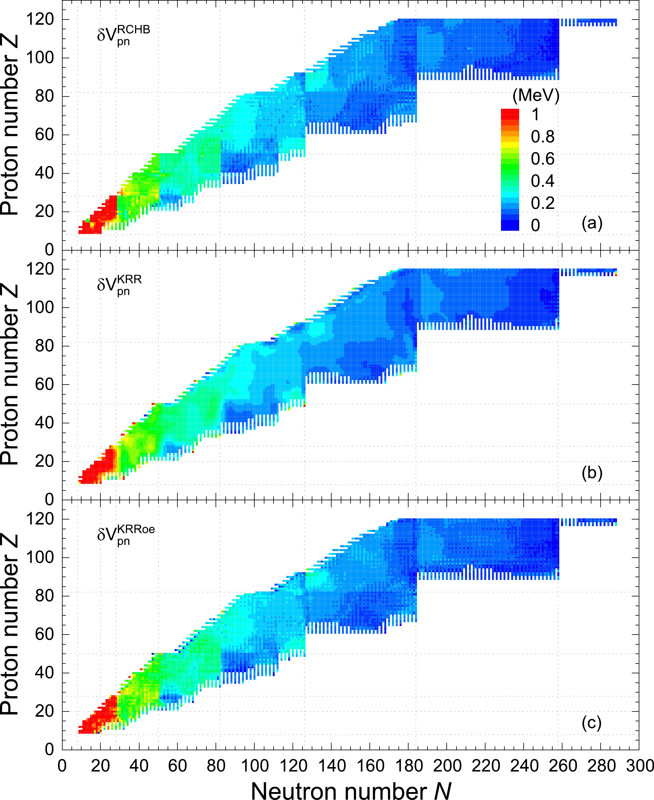
Figure 6. (color online) The extracted empirical proton-neutron interactions from the RCHB mass table (a), in comparison with those from the KRR (b) and KRRoe (c) predictions. The values are scaled by colors.
-
The discussions presented above showed the learning results of the KRR method with optimized hyperparameters. Note that the learning ability of the KRR method may significantly depend on the hyperparameters. Therefore, it is worth investigating how the learning ability changes with different hyperparameters. In the following, comparisons between the optimized KRR results and the learning results obtained using two other sets of hyperparameters
$ (\sigma, \lambda)=(4.0, 1.0\times 10^{-3}) $ and$ (30.0, 1.0\times 10^{-3}) $ are presented. Both rms deviations with respect to the RCHB mass table are less than 2 MeV.For a close look, Fig. 7(a) and Fig. 7(b) show the odd-even mass differences in Ca and Sn isotopic chains obtained by the KRR predictions with the three different sets of hyperparameters, in comparison with those from the RCHB mass table, from the KRRoe predictions, and from the experimental data. It can be seen that both the RCHB theory and the KRRoe predictions reproduce the empirical odd-even mass differences very well. However, all three KRR predictions fail to reproduce the correct staggering in the odd-even mass differences, for both large and small values of the hyperparameter σ. A clear staggering opposite in phase is even given out by the KRR predictions with a small
$ \sigma=4.0 $ . This strange behavior can actually be understood. When the KRR predictions with a small σ are applied, the binding energy of the middle nucleus in Eq. (7) that should have been relatively large (small) owing to pairing correlations is contaminated heavily by correlating the small (large) binding energies of the two neighboring nuclei. If the hyperparameter σ increases, the effective correlation distance increases, resulting in the quenching of odd-even mass differences.
Figure 7. (color online) Odd-even mass differences and empirical proton-neutron interactions of Ca and Sn isotopic chains in the RCHB mass table and the different KRR predictions, as functions of the neutron number. The KRR results include the optimized predictions (KRR), predictions with
$ \sigma=4.0 $ and$ \lambda=1.0\times 10^{-3} $ (KRR*), and predictions with$ \sigma=30.0 $ and$ \lambda=1.0\times 10^{-3} $ (KRR**). The corresponding experimental data [99] and the results given by the KRRoe method are shown for comparison.Figure 7(c) and 7(d) present the empirical proton-neutron interactions in Ca and Sn isotopic chains obtained by the KRR predictions with the three different sets of hyperparameters, in comparison with those from the RCHB mass table and the KRRoe predictions. As shown, upon the overall decrease with the increasing neutron number, the
$\delta V_{{pn}} $ values obtained by the RCHB mass table and the KRRoe predictions exhibit a rapid drop at shell closure$ N=28 $ in Ca and at$ N=82 $ in the Sb isotopic chain. The three KRR predictions can reproduce this overall decrease, but the one with a large hyperparameter$ \sigma=30.0 $ does not exhibit the rapid drop at shell closure. In comparison, the one with a small hyperparameter, i.e.,$ \sigma=4.0 $ , exhibits more fluctuations that appear random. Nevertheless, these different behaviors with different hyperparameters (σ) can be basically understood by considering σ as a measure of the effective correlation distance. -
In summary, the kernel ridge regression method and its extension with odd-even effects have been used to learn the binding energies in the theoretical mass table obtained by the relativistic continuum Hartree-Bogoliubov theory. By investigating the shell effects, one-nucleon and two-nucleon separation energies, odd-even mass differences, and empirical proton-neutron interactions extracted from the learned binding energies, the ability of the machine learning tool to grasp the known physics is discussed.
It is found that the binding energies learned by the KRR method have a 0.96 MeV rms deviation with respect to the 9035 data in the RCHB mass table. The shell effects that are reflected in the differences with the BW formula are well reproduced by the KRR predictions. The evolutions of nucleon separation energies and empirical proton-neutron interactions are also learned by the KRR method effectively. However, the odd-even mass differences cannot be reproduced by the KRR method with a Gaussian kernel at all, even with different hyperparameters. A small hyperparameter σ, which characterizes the effective correlation distance, leads to an odd-even staggering opposite in phase, whereas a large σ results in the quenching of odd-even mass differences. The KRR method with odd-even effects remarkably increases the prediction accuracy to the RCHB mass table; the corresponding rms deviation is 0.17 MeV. Furthermore, the odd-even mass differences can be well reproduced.
It is also necessary to discuss the extrapolation. Generally, all machine-learning approaches lose their predictive power when extrapolating to large distances, and their abilities with the increasing extrapolation should be examined. The extrapolation ability of the KRR approach has been carefully examined in several previous works [62, 63, 65]. These works demonstrate that compared with other machine-learning approaches, the KRR approach loses its extrapolation power in a relatively gentle way with the increasing extrapolation distance.
Finally, concerning the issue of physics learning abilities of the machine learning tools, the present study may provide some insights:
(i) By learning and reproducing the data, the machine leaning tools can grasp some of the physical effects that are reflected in the data and their derived quantities.
(ii) The root-mean-square deviation
$ \sigma_{\mathrm{rms}} $ between the predictions and the data can naturally be a measure of the ability to grasp physical effects. A concrete example is that the KRR predictions with$ \sigma_{\mathrm{rms}}=0.96 $ MeV well reproduce the shell effects reflected in binding energies but fail to reproduce the odd-even mass differences that are mostly less than 1 MeV, whereas the KRRoe predictions with$ \sigma_{\mathrm{rms}}=0.17 $ MeV can well reproduce the odd-even mass differences. However, this does not mean that all the physical effects with the quantity less than$ \sigma_{\mathrm{rms}} $ cannot be learned by the corresponding machine learning tool, e.g., the KRR predictions can reproduce the evolutions of empirical proton-neutron interactions as well.(iii) The model design of machine learning can significantly influence the learning behaviors and effectiveness, and the hyperparameters in a machine learning model may help us to understand the learning performance. The hyperparameter σ in the KRR and KRRoe methods effectively determines the correlation distance between the data and influences the evolution behavior of physical quantities. By including the odd-even effects as prior knowledge, the KRRoe method remodulates the kernel function and significantly increases the accuracy of prediction.
(iv) But not the least, the present analyses on physical effects are only based on the predicted data and their derived quantities. It is more challenging and intriguing to gain some physical insights through the machine learning tools, and some attempts for this aim have been performed [74].
-
The authors greatly appreciate J. Meng for stimulating discussions. The calculations are supported by High-performance Computing Platform of Peking University.
Examination of machine learning for assessing physical effects: Learning the relativistic continuum mass table with kernel ridge regression
- Received Date: 2023-02-13
- Available Online: 2023-07-15
Abstract: The kernel ridge regression (KRR) method and its extension with odd-even effects (KRRoe) are used to learn the nuclear mass table obtained by the relativistic continuum Hartree-Bogoliubov theory. With respect to the binding energies of 9035 nuclei, the KRR method achieves a root-mean-square deviation of 0.96 MeV, and the KRRoe method remarkably reduces the deviation to 0.17 MeV. By investigating the shell effects, one-nucleon and two-nucleon separation energies, odd-even mass differences, and empirical proton-neutron interactions extracted from the learned binding energies, the ability of the machine learning tool to grasp the known physics is discussed. It is found that the shell effects, evolutions of nucleon separation energies, and empirical proton-neutron interactions are well reproduced by both the KRR and KRRoe methods, although the odd-even mass differences can only be reproduced by the KRRoe method.


 DownLoad: