


 Abstract
 HTML
HTML Reference
 Related
 PDF
PDF


-
As the fundamental theory of strong interaction describing more than 99% of visible matter in the universe, quantum chromodynamics (QCD) is successful in the ultraviolet region when the coupling is weak [1, 2]. However, solving nonperturbative QCD physics in the infrared (IR) regime remains a challenge in hadron physics and QCD phase transitions related to chiral symmetry breaking and color confinement. In recent decades, the holographic QCD method based on the anti-de Sitter/conformal field theory (AdS/CFT) correspondence or gauge/gravity duality [3–5] has become an important tool in dealing with nonperturbative QCD problems and has been widely applied in hadron physics and strongly coupled quark matter.
According to the conjecture of AdS/CFT correspondence, it is widely believed that there exists a general holography between D-dimensional quantum field theory (QFT) and (D+1)-dimension quantum gravity, with the extra dimension as an emergent energy scale or renormalization group (RG) flow in the QFT [6]. There have been numerous efforts to construct a non-conformal 5-dimensional holographic QCD model via both top-down and bottom-up approaches, for example, the
$ D_p-D_q $ system from top-down, including the$ D_3-D_7 $ [7] and$ D_4-D_8 $ systems, or the Witten-Sakai-Sugimoto (WSS) model [8, 9]. Regarding the bottom-up approach, the hard-wall model [10] and soft-wall AdS/QCD model or KKSS model [11] established the 5-dimensional framework for light hadron spectra. In the simplest models, such as the KKSS model, the generation of the quark condensate has not been included, and the decoupling of the deep IR from the physics of the mesons is dictated by hand using a soft wall at IR. Progress was made in Refs. [12–15].In the bottom-up method, in order to break the conformal invariance, energy scale dependent operators including IR physics are taken into account. For example, in [16], a z-dependent mass was introduced so that the IR physics can be improved in the soft-wall AdS/QCD model. In a recent paper [17], the authors discussed the effects of the beta function on the mass and melting temperature for scalar glueballs. The chiral condensate was studied from a general point of view in [18]. In [14], the dilaton profile and the potential in the KKSS model action were modified by a quartic term to obtain the chiral symmetry breaking. In [19], the scalar mass was dependent on the holographic radial coordinate for studying the meson spectra in the model, and a generalized study to consider interactions was performed in [20].
The anomalous dimension has also been introduced in bottom-up holographic models to break conformal symmetry. In the Gubser model [21–24], an anomalous dimension of gluon condensation has been taken into account. The beta function for scalar gluballs was introduced in [25]. The scaling dimensions and the gluon field propagator were studied in [26]. A warp factor related to the photon field was introduced in [27] for the electromagnetic pion form factor as well as the pion radius. In [28], an anomalous dimension of an operator for fermions at the boundary was taken into account to compute the corresponding structure functions. In the D3/D7 system, it has been phenomenologically adjusted to include a running anomalous dimension γ for the quark quark condensate [29–31]. From the AdS/CFT correspondence, the nonzero quark condensate is dual to the scalar field in the AdS background suffering an instability. When the scalar field mass is
$ m^2=-4 $ , it passes through the Breitenlohner-Freedman bound [32].Systematic frameworks such as the improved holographic QCD (IhQCD) model [33, 34], the V-QCD model [35], and the dynamical holographic QCD model [36, 37] have been developed to incorporate linear confinement and chiral symmetry breaking. The improved holographic QCD (IhQCD) model [33, 34] and the V-QCD model are embedded in the running coupling from UV to IR in the dilation potential. In the simplest version of the dynamical holographic QCD model [36, 37], the KKSS model action describing the flavor physics is added on a dilaton-graviton coupled background. Thus, the AdS
$ _5 $ metric is automatically deformed by the gluon condensation and further deformed by the chiral condensation. In this framework, both the chiral symmetry breaking and linear confinement can be realized; therefore, in the produced light-flavor hadron spectra, one can read the information of chiral symmetry breaking: the$140 ~{\rm MeV}$ pseudo Nambu-Goldstone boson, i.e., the pion, and the splitting between the chiral partners, as well as the linear confinement information through the linear Regge behavior of higher excitation states. It was difficult to reconcile the light-flavor hadron spectra and pion form factor in [37]. To improve this part, in this work, we consider the anomalous 5-dimension mass correction of the scalar field from QCD running coupling. In this paper, we extend the model so that it includes the dynamics of gauges. We input it through an assumption for the running of the anomalous dimension of the quark antiquark γ. We take the running of γ from the perturbative two loop result for$ S U(3) $ gauge theory with two flavors, i.e.,$ N_f=2 $ .It is found that with the anomalous 5-dimension mass correction of the scalar field, the light flavor hadron spectra and pion form factor can be described well simultaneously. In particular, the ground state and lower excitation states of the scalar, pseudo scalar, and axial vector meson spectra are improved; however, the vector meson spectra are not sensitive to the anomalous 5-dimension mass correction of the scalar field. The remainder of this paper is organized as follows. In Sec. II, we briefly introduce the dynamical holographic QCD model. In Sec. III, we introduce the anomalous dimension of the scalar field, and in Sec. V, we present numerical results for the hadron spectra and pion form factor. Finally, we summarize the paper and present conclusions in Sec. VI.
-
Following Refs. [37, 38], one can couple the Einstein-Dilaton system and the KKSS action, which are assumed to describe the gluonic dynamics and the flavor dynamics, respectively. Then, we have the system
$ S = S_{G}+ \frac{N_f}{N_c} S_{f}, $

(1) with the gluon background part
$ S_{G} $ and flavor part$ S_{f} $ of the following forms:$ \begin{eqnarray} && S_{G} = \frac{1}{16\pi G_5}\int {\rm d}^5x\sqrt{g_s} {\rm e}^{-2\Phi}\big(R+4\partial_M\Phi\partial^M\Phi-V_G(\Phi)\big), \end{eqnarray} $

(2) $ \begin{aligned}[b]S_{f}=&-\int {\rm d}^5x {\rm e}^{-\Phi(z)} \sqrt{g_s}Tr\Big(|DX|^2+V_X(|X|,\Phi) \\&+\frac{1}{4g_5^2}(F_L^2+F_R^2)\Big) . \end{aligned} $

(3) Here, we have taken
$S_f=S_{\rm KKSS}$ , i.e., the simplest version for the flavor part. In Eq. (3), Φ is the dilaton field,$ X\equiv X^{\alpha \beta} $ is a matrix-valued scalar field with$ \alpha,\beta $ being the flavor indexes,$ g_s \equiv \text{det}(g^s_{\mu\nu}) $ is the determinant of the metric in the string frame,$ V_G $ is the dilaton potential, and$ V_X $ is the scalar potential, which includes the interaction between X and Φ (strictly speaking, it is an extension of the original KKSS model).$ F_L $ and$ F_R $ represent the gauge strengths of the left-handed guage potential$ L^{M}= L^{Ma} t^a $ and right-handed gauge potential$ R^{M}= R^{Ma} t^a $ $ \begin{aligned}[b] F_{L}^{MN}=\partial^{M}{L^{N}}-\partial^{N}{L^{M}}-{\rm i} [L^{M},L^{N}],\end{aligned} $

$ \begin{aligned}[b] F_{R}^{MN}=\partial^{M}{R^{N}}-\partial^{N}{R^{M}}-{\rm i} [R^{M},R^{N}], \end{aligned} $

(4) with
$ t^a $ the generators of the group considered, for which we have Tr$ [t^{a}t^{b}]=\delta^{ab}/2 $ . One can transform the left-handed gauge field L and the right-handed gauge field R into the vector (V) and axial-vector (A) fields with$ L^{M}=V^{M}+A^{M} $ and$ R^{M}=V^{M}-A^{M} $ .$ DX $ represents the covariant derivative, which takes the form$ \begin{array}{*{20}{l}} D^M X=\partial^M X-{\rm i} L^M X+ {\rm i} X R^M. \end{array} $

(5) One of the main tasks to build the holographic model is to solve the gravity background, which is dual to the vacuum. In this work, we consider that all the current quarks are degenerate. Thus, we take a simple ansatz for the background part of X, i.e.,
$X=\dfrac{\chi}{2} I$ , with I being the identity matrix. Because the vacuum does not carry other nonzero quantum numbers, we assume the gauge fields to be zero in the vacuum and consider them as perturbations above the vacuum. Therefore, in the background part, only the metric, the dilaton field, and the diagonal part of the scalar field χ appear. By inserting the above ansatz into the action, we obtain an effective expression in terms of Φ and χ as follows:$ \begin{aligned}[b] S_{\rm vac} =& \frac{1}{16 \pi G_5} \int {\rm d}^5 x \sqrt{g_s} \bigg\{ {\rm e}^{-2\Phi}[R +4\partial_M\Phi \partial^M \Phi - V_G(\Phi)] \\ &- \lambda {\rm e}^{-\Phi} \left(\frac{1}{2} \partial_M\chi \partial ^M \chi + V_C(\chi,\Phi)\right)\bigg\}. \\[-13pt]\end{aligned} $

(6) Here, we have redefined the coupling between the two sectors as
$ \lambda\equiv \dfrac{16\pi G_5 N_f}{ N_c} $ (for simplicity, we take the AdS radius$ L=1 $ ). Considering the Lorenzian symmetry of the vacuum, one can take the ansatz of the metric as$ \begin{eqnarray} g^s_{MN}=b_s^2(z)(dz^2+\eta_{\mu\nu}dx^\mu dx^\nu), \; \; b_s(z)\equiv {\rm e}^{A_s(z)}. \end{eqnarray} $

(7) Here, z is the holographic dimension, and
$ z=0 $ is the 4D boundary.$ \eta_{\mu\nu} $ is the metric of the Minkowski space with$ \eta_{00}=-1 $ . Then, it is not difficult to derive the equation of motion from the Einstein equations and the field equations:$ \begin{eqnarray} -A''_s+A'^2_s+\frac{2}{3}\Phi''-\frac{4}{3}A'_s\Phi' -\frac{\lambda}{6}{\rm e}^{\Phi}\chi'^{2}&=0, \end{eqnarray} $

(8) $ \begin{aligned}[b] \Phi''&+(3A'_s-2\Phi')\Phi'-\frac{3\lambda}{16} {\rm e}^{\Phi}\chi'^{2} -\frac{3}{8} {\rm e}^{2A_s-\frac{4}{3}\Phi}\partial_{\Phi}\Big(V_G(\Phi) \\& +\lambda {\rm e}^{\frac{7}{3}\Phi}V_C(\chi,\Phi)\Big)=0, \end{aligned} $

(9) $ \begin{eqnarray} \chi''+(3A'_s-\Phi')\chi'- {\rm e}^{2A_s}V_{C,\chi}(\chi,\Phi)&=0. \end{eqnarray} $

(10) According to the analysis in Refs. [37, 38], in order to incoorperate the linear spectrum, the linear potential, and the chiral symmetry breaking, one can take the following field configurations:
$ \begin{eqnarray} &&\Phi(z)=\mu_G^2z^2, \end{eqnarray} $

(11) $ \begin{eqnarray} &&\chi'(z)=\sqrt{8/\lambda}\mu_G {\rm e}^{-\Phi/2}(1+c_1 {\rm e}^{- \Phi}+c_2 {\rm e}^{-2\Phi}), \end{eqnarray} $

(12) where
$ \mu_G $ is a model parameter related to the Regge slope of the spectrum. The quadratic form of the dilaton field is taken from the original KKSS model. It turns out to be responsible for the linear spectrum of light mesons. The specific form of$ \chi^\prime $ is introduced phenomenologically, which leads to$A_s^\prime\rightarrow 0, A_s\rightarrow \rm Const$ when z approaches infinity and is responsible for the linear part of the quark-antiquark potential (the linear confinement from another point of view). Furthermore, in order to describe the chiral condensate, the asymptotic behavior of χ should take the following form:$ \begin{eqnarray} \chi(z) \stackrel{z \rightarrow 0}{\longrightarrow} m_q \zeta z+\frac{\sigma}{\zeta} z^3. \end{eqnarray} $

(13) Thus, we have the two coefficients
$c_1= -2+ $ $ \dfrac{5\sqrt{2\lambda}m_q\zeta}{8\mu_G}+\dfrac{3\sqrt{2\lambda}\sigma}{4\zeta \mu_G^3}, ~~ c_2=1-\dfrac{3\sqrt{2\lambda}m_q\zeta}{8\mu_G}-\dfrac{3\sqrt{2\lambda}\sigma}{4\zeta \mu_G^3}$ . Here,$ m_q $ and σ are the current quark mass and chiral condensate, respectively. ζ is a normalization constant, which is introduced by matching the 5D results of the two-point function of the scalar operator$ \bar{q}q $ to the 4D perturbative calculations [18].With all these considerations, one can take proper values of the parameters
$ \mu_G, m_q, \sigma,\lambda $ and calculate the metric, as well as the dilaton and scalar potentials$ V_G, V_C $ , from the equations of motion. Generally, they are functions of z, similar to$ \Phi, \chi $ . After solving all the functions, one may extract the dilaton and the scalar potential$ V_G, V_{c,\chi} $ . To do so, we assume that the interaction between Φ and χ takes a simple form$V_{c,\chi}={\rm e}^{f(\Phi)}V_{c,\chi}(\chi)$ and simply take$ f(\Phi)=-\Phi/2+\ln(1+\Phi)/2 $ . Then, one can easily extract the asymptotic behavior of$ V_c(\chi) $ as$ \begin{eqnarray} V_{c}(\chi)=\frac{1}{2}M^2\chi^2+o(\chi^2), \end{eqnarray} $

(14) with the 5D mass
$ M^2=-3 $ , which satisfies the operator dimension Δ and 5D mass relation$ M^2=\Delta(\Delta-4) $ for scalar operator$ \bar{q}q $ with$ \Delta=3 $ . -
The above form can be considered as defined at the ultra-UV scale, where the dimension of
$ \bar{q}q $ is$ \Delta=3 $ . However, according to the perturbative calculation in 4D QCD, the dimension of the scalar operator$ \bar{q}q $ would obtain corrections, i.e., the anomalous dimension γ, when considering quantum fluctuations. Generally, the anomalous dimension depends on the energy scale. Considering that the duality is valid at strong coupling other than at ultra-UV, one might expect an anomalous dimension correction to the operator dimension.With a nonzero anomalous dimension γ, the dimension of the operator
$ \bar{q}q $ becomes$ \Delta-\gamma $ . From the relation between the 5D mass and the operator dimension, the mass of the dual 5D scalar field is$ \begin{array}{*{20}{l}} \tilde{M}^2=M^2+\Delta M^2=(\Delta-\gamma)(\Delta-\gamma-4). \end{array} $

(15) Correspondingly, the asymptotic expansion of χ in Eq. (13) becomes
$ \begin{eqnarray} \chi(z) \stackrel{z \rightarrow 0}{\longrightarrow} m_q \zeta z^{1+\gamma}+\frac{\sigma}{\zeta} z^{3-\gamma}. \end{eqnarray} $

(16) Phenomenologically, one can take a constant value of γ as in Ref. [21], work out
$ \Delta M^2 $ , and solve the corrections to the background metric and fields. To be more careful, the anomalous dimension is generally a function of the energy scale. In the 5D description, because the holographic direction can be mapped to the energy scale, one might transfer the energy scale dependence of the anomalous dimension to the 5th dimension evoloution of the anomolous dimension. Thus, γ should be a function of the holographic dimension, i.e., as a function$ \gamma(z) $ other than a constant. Then, the asymptotic expansion of$ \chi(z) $ becomes$ \begin{eqnarray} \chi(z) \stackrel{z \rightarrow 0}{\longrightarrow} m_q \zeta z^{1+\gamma(z)}+\frac{\sigma}{\zeta} z^{3-\gamma(z)}. \end{eqnarray} $

(17) The 5D mass then effectively becomes
$ \begin{array}{*{20}{l}} \tilde{M}^2=[\Delta-\gamma(z)][\Delta-\gamma(z)-4]. \end{array} $

(18) Then, if the 5D mass in the potential
$ V_{C,\chi}(\chi,\Phi) $ is modified to the above form, the corrections from the anomalous dimension can be solved. However, because$ V_{C,\chi}(\chi,\Phi) $ is numerically obtained in the previous works, i.e., Refs. [37, 38], it is not directly to add the correction in this way. Instead, we will introduce the corrections in an effective way. Comparing Eq. (17) with Eq. (13), one might expect minor corrections to the previous model, by replacing the constants$ c_1, c_2 $ as functions of z. Therefore, we have$ \begin{eqnarray} &&\Phi(z)=\mu_G^2z^2, \end{eqnarray} $

(19) $ \begin{eqnarray} &&\chi'(z)=\sqrt{8/\lambda}\mu_G {\rm e}^{-\Phi/2}(1+c_1(z) {\rm e}^{- \Phi}+c_2(z) {\rm e}^{-2\Phi}) . \end{eqnarray} $

(20) The functions
$ c_1(z) $ and$ c_2(z) $ can be obtained by comparing the UV asymptotic expansion of Eq. (20) to Eq. (17), and they have the following forms:$ \begin{eqnarray} c_1&=&-2+\frac{5\sqrt{2\lambda}m_q {\rm e}^2 z^{\gamma(z)}\zeta}{8\mu_G}+\frac{3\sqrt{2\lambda}\sigma z^{-\gamma(z)}}{4{\rm e}^2\zeta \mu_G^3}, \end{eqnarray} $

(21) $ \begin{eqnarray} c_2&=&1-\frac{3\sqrt{2\lambda}m_q{\rm e}^2 z^{\gamma(z)}\zeta}{8\mu_G}-\frac{3\sqrt{2\lambda}\sigma z^{-\gamma(z)}}{4{\rm e}^2\zeta \mu_G^3} \end{eqnarray} $

(22) Here, the factor
$ e^2 $ is to guarantee that the dimension recovers 3 at ultra UV. In this way, the asymptotic behavior of χ becomes Eq. (20), and the anomalous dimension is effectively introduced.To solve the dependence of z of
$ \gamma(z) $ , one has to consider the constraints from the 4D perturbative calculations. The running of the gauge coupling in QCD theory is controlled by the β function as follows:$ \begin{eqnarray} \mu { {\rm d} \alpha \over {\rm d} \mu} = \beta(\alpha) . \end{eqnarray} $

(23) From the 4D one loop results, the anomalous dimension of the operator
$ \bar{q}q $ takes the form$ \gamma =\frac{ 3 (N_c^2-1)} { 4 N_c \pi} \alpha\,. $

(24) We assume that the inverse of the renormalization scale
$ \mu^{-1} $ corresponds to the z coordinate and Eq. (23) becomes$ -z \frac{d \alpha}{dz}=\beta(\alpha). $

(25) In this work, we consider the one loop perturbative calculation only; thus, we have
$ \begin{eqnarray} \beta(\alpha)= - b_0 \alpha^2 , \end{eqnarray} $

(26) with
$ b_0 = \frac{1}{ 6 \pi} (11 N_c - 2N_f). $

(27) The perturbative results are valid at high energy scales only. To extend it to the IR region, we impose a simple extrapolation following Refs. [39–41], which reads
$ \begin{eqnarray} \beta(\alpha)= - b_0 \alpha^2(1-\alpha/\alpha_0)^2 . \end{eqnarray} $

(28) Here,
$ \alpha_0 $ is the IR fix point, which is considered as a model parameter in this work. Taking the above form, one can solve the beta function and the z dependence of γ and then solve the equations of motion, i.e., Eqs. (8)– (10).Given the non-perturbative dominant physics for hadrons, one might expect that the UV perturbative part contributes less to the final results; thus, we also consider two simple models of the anomalous dimensions for comparison: (a) We take
$\gamma(z)=-\dfrac{3}{2}({\rm e}^{-\Phi^2/2}-1)$ and replace$ m_q,\sigma $ with$m_q z^{\gamma(z)}[\dfrac{1}{2}(1+\gamma(z))+\ln(z)\gamma^\prime(z)],~~ \sigma z^{-\gamma(z)}[\dfrac{1}{2}(3- \gamma(z))- \ln(z)\gamma^\prime(z)]$ ; (b) we also take a constant γ.Finally, to solve the models, we need to fix the parameters. First, in this work, we focus on the case of
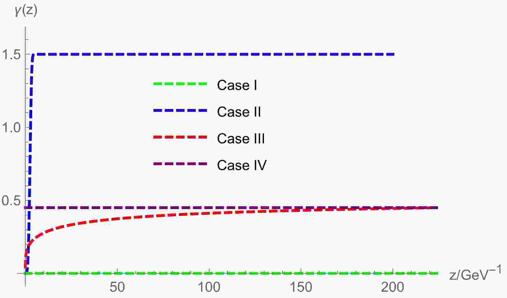
$ N_c=3, N_f=2 $ . The value of the parameter$ \mu_G $ describes the Regge slope, and it can be fixed as$ \mu_G=0.43\rm{GeV} $ . Follwoing Ref. [37], we take$G_5=0.75 $ ,$m_q=5 ~\rm{MeV}, \sigma=(240~\rm{MeV})^3$ (Model IB in Refs. [37, 38]). The coupling at IR fixed point$ \alpha_0 $ is taken to be$ 1 $ . With these parameters, taking the initial condition$ \alpha(z=1/M_Z)=0.1184 $ , one can solve the dynamic$ \gamma(z) $ from the beta function as indicated by the red dashed line in Fig. 1. By inserting the solution of$ \gamma(z) $ into the equation of motion, one can solve the warp factor of the metric$ A_s $ and the scalar field. The results are given as the red dashed lines in Fig. 2.
Figure 1. (color online) The anomalous dimension as a function of the holographic dimension
$ \gamma(z) $ .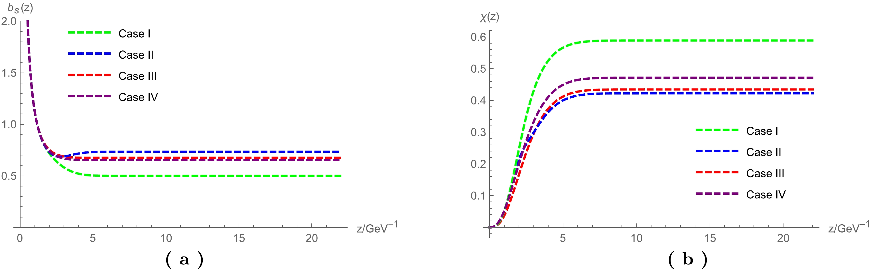
Figure 2. (color online) The warp factor
$ b_s(z) $ (a) and the scalar field$ \chi(z) $ (b).As mentioned above, in addition to the dynamic
$ \gamma(z) $ from the beta function, we considered the other three cases. Here, we call the case without anomalous dimension corrections "Case I" (the same as Model IB in Ref. [37]), the case with modeling of$\gamma(z)=-\dfrac{3}{2}({\rm e}^{-\Phi^2/2}-1)$ "Case II," the case with the dynamical evolution of$ \gamma(z) $ from the beta function "Case III," and the case with a constant$ \gamma=0.45 $ (around the dynamical value at large z) "Case IV." The behaviors of$ \gamma(z) $ in different models are given in Fig. 1. The solutions of$ b_s $ and χ are obtained by numerically solving the equation of motion and are shown in Fig. 2. From the figure, one can easily see that$ b_s $ in all the cases behaves as$ b_s\simeq 1/z $ , guaranteeing the asymptotic AdS condition. At large z, i.e., in the IR region,$ b_s $ tends to different constants in different models (0.5, 0.73, 0.68, and 0.65 for Cases I, II, III, and IV respectively), which is responsible for the linear part of the quank potential. In the UV region, the solutions of$ \chi(z) $ are constrained by the UV expansion. Additionally, in the IR region, it tends to constants for the different models. Roughly, one can numerically verify that the values of$ b_s \chi $ at large z are approximately$ 0.3 $ for the different models.Up to now, we have modeled the anomalous dimension in the dynamical holographic QCD model, and we have solved the background fields describing the vacuum properties. Next, we will continue to study the excitations on the vacuum.
-
After solving the background metric and fields, one can study the properties of the mesons as perturbations on the vacuum. For the scalar channel, we take
$X=(\dfrac{\chi}{2}+s){\rm e}^{{\rm i} 2\pi^a t^a}$ , with$ s, \pi $ being the scalar and pseudo-scalar perturbation, respectively, considering$ s,\pi $ as perturbations. Because the vaccum does not have a background field in the vector channel, we simply take the vector perturbation as$ v_\mu $ and the axial vector perturbation as$ a_\mu $ . By calculating the two-point current-current correlation function of the corresponding field, one can obtain the masses of the mesons from their poles. Equivalently, with an example shown in Appendix A, it can be obtained by solving the following Schrödinger-like equations for$ s,\pi,v_\mu,a_\mu $ $ -s''_n+V_s(z)s_n=m_n^2s_n, $

(29) $ -\pi''_n+V_{\pi,\varphi}\pi_n=m_n^2(\pi_n-{\rm e}^{A_s}\chi\varphi_n), $

(30) $ -\varphi''_n+ V_{\varphi} \varphi_n=g_5^2 {\rm e}^{A_s}\chi(\pi_n-{\rm e}^{A_s}\chi\varphi_n), $

(31) $ -v''_n+V_v(z)v_n=m_{n,v}^2v_n, $

(32) $ -a''_n+V_a a_n = m_n^2 a_n, $

(33) with the potentials
$V_s=\frac{3A''_s-\Phi''}{2}+\frac{(3A'_s-\Phi')^2}{4}+{\rm e}^{2A_s}V_{C,\chi\chi}, $

(34) $ \begin{aligned}[b] V_{\pi,\varphi}=&\frac{3A''_s-\Phi''+2\chi''/\chi-2\chi'{2}/\chi^2}{2} \\& +\frac{(3A'_s-\Phi'+2\chi'/\chi)^2}{4}, \end{aligned} $

(35) $ V_{\varphi} = \frac{A''_s-\Phi''}{2}+\frac{(A'_s-\Phi')^2}{4}, $

(36) $ V_v=\frac{A''_s-\Phi''}{2}+\frac{(A'_s-\Phi')^2}{4} \; , $

(37) $ V_a = \frac{A'_s-\Phi'}{2}+\frac{(A'_s-\Phi')^2}{4}+g_5^2 e^{2A_s}\chi^{2} . $

(38) Here, the longitudinal part
$ a^{l}_\mu $ of the axial vector perturbations couples with the pseudo-scalar part, and we have imposed$ a^{l}_\mu=\partial_\mu \varphi $ . Once one obtains the background solution, the masses of the mesons can be obtained by numerically solving the above equations.It is also easy to extract the decay constants
$f_\pi,~ F_{\rho_n}, F_{a_1,n}$ following Refs. [37, 38], and they take the following forms:$ \begin{eqnarray} f_\pi^2&&=-\frac{N_f}{g_5^2N_c}{\rm e}^{A_s-\Phi}\partial_z A(0,z)|_{z\rightarrow0}, \end{eqnarray} $

(39) $ \begin{eqnarray} F_{\rho_n}^2&&=\frac{N_f}{g_5^2N_c}({\rm e}^{A_s-\Phi}\partial_z V_n(z)|_{z\rightarrow0})^2, \end{eqnarray} $

(40) $ \begin{eqnarray} F_{a_1,n}^2&&=\frac{N_f}{g_5^2N_c}({\rm e}^{A_s-\Phi}\partial_z A_n(z)|_{z\rightarrow0})^2. \end{eqnarray} $

(41) Here
$ A(0,z),~V_n(z),~ A_n(z) $ satisfy$ \begin{eqnarray} (-{\rm e}^{-(A_s-\Phi)}\partial_z({\rm e}^{A_s-\Phi}\partial_z)+g_5^2 {\rm e}^{2A_s}\chi^2)A(0,z)=0, \end{eqnarray} $

(42) $ \begin{eqnarray} (-{\rm e}^{-(A_s-\Phi)}\partial_z({\rm e}^{A_s-\Phi}\partial_z)-m_{\rho,n}^2)V_n(z)=0, \end{eqnarray} $

(43) $ \begin{eqnarray} (-{\rm e}^{-(A_s-\Phi)}\partial_z({\rm e}^{A_s-\Phi}\partial_z)+g_5^2 {\rm e}^{2 A_s}\chi^2-m_{a_1,n}^2)A_n(z)=0, \end{eqnarray} $

(44) with the boundary condition
$ A(0,0)=1,~ \partial_z A(0,\infty)=0 $ ,$ V_n(0)=0, ~ \partial_zV_n(\infty)=0 $ ,$ A_n(0)=0, ~ \partial_zA_n(\infty)=0 $ and normalized as$ \int {\rm d} z {\rm e}^{A_s-\Phi} V_m V_n=\int {\rm d} z {\rm e}^{A_s-\Phi} A_m A_n=\delta_{mn}. $ The pion form factor can also be derived as in Refs. [37, 38]:$ \begin{aligned}[b] f_\pi^2 F_\pi(Q^2)=&\frac{N_f}{g_5^2N_c}\int {\rm d}z {\rm e}^{A_s-\Phi} V(q^2,z) \big\{ (\partial_z\varphi)^2\\&+g_5^2\chi^2 {\rm e}^{2A_s} (\pi-\varphi)^2\big\}, \end{aligned} $

(45) where
$ Q^2=-q^2 $ , and$ V(q^2,z),\pi(z),\varphi(z) $ satisfy$ \begin{eqnarray} (-{\rm e}^{-(A_s-\Phi)}\partial_z({\rm e}^{A_s-\Phi}\partial_z )+q^2)V(q^2,z)=0, \end{eqnarray} $

(46) $ \begin{eqnarray} -{\rm e}^{-(3A_s-\phi)}\partial_z({\rm e}^{3A_s-\phi}\chi^2 \partial_z)\pi-m_{\pi,n}^2\chi^2(\pi-\varphi)=0, \end{eqnarray} $

(47) $ \begin{eqnarray} -{\rm e}^{-(A_s-\phi)}\partial_z({\rm e}^{A_s-\phi} \partial_z)\varphi-g_5^2\chi^2{\rm e}^{2A_s}(\pi-\varphi)=0, \end{eqnarray} $

(48) with the boundary condition
$V(q^2,0)=1,\partial_zV(q^2, ~ \infty)=0, \pi(0)=0, ~ \partial_z\pi(\infty)=0, ~ \varphi(0)=0,\varphi(\infty)=0$ and normalized as$ \begin{eqnarray} \frac{N_f}{g_5^2 N_c f_\pi^2}\int {\rm d}z {\rm e}^{A_s-\Phi} \big\{ (\partial_z\varphi)^2+g_5^2\chi^2 {\rm e}^{2A_s} (\pi-\varphi)^2\big\}=1. \end{eqnarray} $

(49) One can also derive the effective coupling between ρ and π as
$ \begin{eqnarray} g_{n\pi\pi}=g_5 \frac{\int {\rm d}z {\rm e}^{A_s-\Phi} V_n \big\{ (\partial_z\varphi)^2+g_5^2\chi^2 {\rm e}^{2A_s} (\pi-\varphi)^2\big\}}{\int {\rm d}z {\rm e}^{A_s-\Phi} \big\{ (\partial_z\varphi)^2+g_5^2\chi^2 {\rm e}^{2A_s} (\pi-\varphi)^2\big\}}, \end{eqnarray} $

(50) where
$ V, \pi, \varphi $ are the wave functions of the corresponding states.Once one knows the dual background solution, the above equations can be solved, and these quantites can be extracted using the above formulae. We discuss the results in Sec. V.
-
After solving the background fields, we can numerically obtain the masses of the mesons, the decay constants, and the form factors. As mentioned in Sec. III, we consider the realistic case and take
$N_c=3,~ N_f=2$ . By taking the parameter set of Model IB with$\mu_G=0.43~\rm{GeV}$ and$m_q=5~\rm{MeV}, \sigma=(240~\rm{MeV})^3$ as in our previous work [37, 38], one can solve the equation of motions and obtain the numerical results. To investigate the effect from the anomalous dimension, we choose three different cases: Case-I: Model IB in Refs. [37, 38], with$ \gamma=0 $ ; Case-II: Model IB with modeling of$ \gamma(z) $ taking the form of$ \gamma(z)=-\frac{3}{2}({\rm e}^{-\Phi^2/2}-1) $ ; Case-III: Model IB with dynamical$ \gamma(z) $ solving from running coupling; and Case-IV: Model IB with a constant$ \gamma=0.45 $ . -
In this work, we consider the anomalous dimension of the
$ \bar{q}q $ operator only. Therefore, the most relevant sector is the scalar sector. In this section, we study the corrections to the scalar and pseudo-scalar mesons, i.e., the$ f_0 $ meson and the pions. The numerical results for the ground states and excitation states for scalar meson$ f_0 $ and the pseudo-scalar meson pions π are presented in Tables 1 and 2 and shown in Fig. 3 for the above three cases. The parameter set Model IB (Case I) is fixed by fitting$m_{\pi}=140~ {\rm MeV}$ , and in Model IB, the ground state mass of the scalar is$231~{\rm MeV}$ , which is less than half of the experimental result. When the anomalous dimension for the scalar field is taken into account, the ground state mass of the scalar is significantly improved, to$488~{\rm MeV}$ ,$539~{\rm MeV}$ ,$609~\rm{MeV}$ for Case-II, Case-III, and Case IV, respectively. As indicated by Tables 1 and 2 and Fig. 3, the low excitation state masses in Model IB are far heavier than the experimental result, whereas in the case with the correction of the anomalous dimension for the scalar field, the low excitation state masses are closer to the experimental results. It is interesting to see from Fig. 3(a) that, by a simple implement of the anomalous dimension, the scalar mass spectra could be significantly improved, especially for Case III when the anomalous dimension is solved dynamically.n $ f_0 $ Exp./MeV

Case-I/MeV Case-II/MeV Case-III/MeV Case-IV/MeV 1 $ 550^{+250}_{-150} $ 

231 488 539 609 2 $ 980 \pm 10 $ 

1106 1000 1043 1040 3 $ 1350 \pm 150 $ 

1395 1267 1366 1357 4 $ 1505 \pm 6 $ 

1632 1591 1620 1608 5 $ 1873 \pm 7 $ 

1846 1848 1837 1824 6 $ 1992 \pm 16 $ 

2039 2063 2030 2016 7 $ 2103 \pm 8 $ 

2215 2249 2206 2192 8 $ 2314 \pm 25 $ 

2376 2410 2367 2355 Table 1. The experimental and predicted mass spectra for scalar mesons
$ f_0 $ . Case-I: Model-IB with$ \gamma=0 $ , Case-II: Model-IB with model$ \gamma(z) $ taking the form of$\gamma(z)=-\dfrac{3}{2}({\rm e}^{-\Phi^2/2}-1)$ , Case-III: Model-IB with dynamical$ \gamma(z) $ solving from running coupling, and Case-IV: Model IB with a constant$ \gamma=0.45 $ . The experimental data are taken from Ref. [42], with a selection scenario following Ref. [14].n π Exp./MeV Case-I/MeV Case-II/MeV Case-III/MeV Case-IV/MeV 1 $ 140 $ 

140 146 158 109 2 $ 1300 \pm 100 $ 

1600 1408 1410 1415 3 $ 1816 \pm 14 $ 

1897 1873 1821 1841 4 $ 2070 $ 

2116 2123 2070 2096 5 $ 2360 $ 

2299 2313 2264 2289 Table 2. The experimental and predicted mass spectra for pseudoscalar mesons π. Case-I: Model-IB with
$ \gamma=0 $ , Case-II: Model-IB with model$ \gamma(z) $ taking the form of$\gamma(z)=-\dfrac{3}{2}({\rm e}^{-\Phi^2/2}-1)$ , Case-III: Model-IB with dynamical$ \gamma(z) $ solving from running coupling, and Case-IV: Model IB with a constant$ \gamma=0.45 $ . The experimental data are taken from Ref. [42], with a selection scenario following Ref. [14].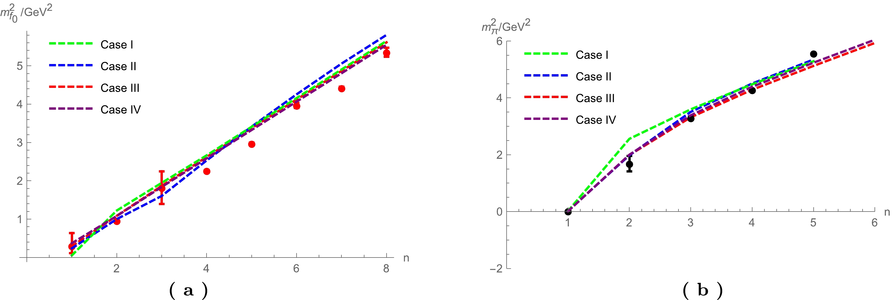
Figure 3. (color online) Spectra of scalars (a) and pseudoscalars (b). Case-I: Model-IB with
$ \gamma=0 $ , Case-II: Model-IB with model$ \gamma(z) $ taking the form of$\gamma(z)=-\dfrac{3}{2}({\rm e}^{-\Phi^2/2}-1)$ , Case-III: Model-IB with dynamical$ \gamma(z) $ solving from running coupling, and Case-IV: Model IB with a constant$ \gamma=0.45 $ . The red and black dots are experimental data, taken from Ref. [42], with a selection scenario following Ref. [14].For the pions, from Fig. 3(b), it is easy to see a similar improvement for the low lying states. The results with the anomalous dimension are far closer to the experimental data for the low lying states. For the higher excitations, all the models tend to give close results. However, it should be pointed out that to show the effects of the anomalous dimension, we fix all the parameters as in Case I, in which the anomalous dimension is not added. Therefore, the results of the ground state of pions are different from the experimental data for Cases II, III, and IV. The deviation for Case II is within
$7$ %, and that for Case III is within$14$ %. For Case IV, the deviation is larger, i.e., approximately$22$ %. For the second excitation states of pions, with the corrections from the anomalous dimension, the results of Cases II, III, and IV become far closer to the experimental data. For even higher excitations, the relative differences of all the cases become small. From the results, we see that although the anomalous dimension is not directly related to the pseudo scalar sector, it can improve the model predicted spectrum indirectly by modifying the background metric and field configuration. -
Next, we consider the corrections from the anomalous dimension of the scalar operator to the vector and axial vector sectors, although this effect is indirect. The numerical results are given in Tables 3 and 4 and Fig. 4. From Table 3, the anomalous dimension would reduce the masses of the lower excitations of ρ, but with only an amount of less than
$7$ %. As for the higher excitations, the differences of different models are even smaller, i.e., less than$0.1$ %. This is mainly because the dominant effect for the ρ spectra is the dilaton field, from which the linearity of the spectrum comes.n ρ Exp./MeV Case-I/MeV Case-II/MeV Case-III/MeV Case-IV/MeV 1 $ 775.5 \pm 1 $ 

771 729 737 741 2 $ 1282 \pm 37 $ 

1143 1135 1136 1137 3 $ 1465 \pm 25 $ 

1431 1423 1425 1426 4 $ 1720 \pm 20 $ 

1670 1663 1665 1666 5 $ 1909 \pm 30 $ 

1878 1873 1874 1875 6 $ 2149 \pm 17 $ 

2065 2061 2062 2062 7 $ 2265 \pm 40 $ 

2237 2234 2234 2235 Table 3. The experimental and predicted mass spectra for vector mesons ρ. Case-I: Model-IB with
$ \gamma=0 $ , Case-II: Model-IB with model$ \gamma(z) $ taking the form of$\gamma(z)=-\dfrac{3}{2}({\rm e}^{-\Phi^2/2}-1)$ , Case-III: Model-IB with dynamical$ \gamma(z) $ solving from running coupling, and Case-IV: Model IB with a constant$ \gamma=0.45 $ . The experimental data are taken from Ref. [42], with a selection scenario following Ref. [14].n $ a_1 $ Exp./MeV

Case-I/MeV Case-II/MeV Case-III/MeV Case-IV/MeV 1 $ 1230 \pm 40 $ 

1316 1222 1163 1232 2 $ 1647 \pm 22 $ 

1735 1676 1649 1707 3 $ 1930^{+30}_{-70} $ 

1969 1971 1926 1980 4 $ 2096 \pm 122 $ 

2163 2178 2132 2181 5 $ 2270^{+55}_{-40} $ 

2336 2356 2311 2358 Table 4. The experimental and predicted mass spectra for axial vector mesons
$ a_1 $ . Case-I: Model-IB with$ \gamma=0 $ , Case-II: Model-IB with model$ \gamma(z) $ taking the form of$\gamma(z)=-\dfrac{3}{2}({\rm e}^{-\Phi^2/2}-1)$ , Case-III: Model-IB with dynamical$ \gamma(z) $ solving from running coupling, and Case-IV: Model IB with a constant$ \gamma=0.45 $ . The experimental data are taken from Ref. [42], with a selection scenario following Ref. [14].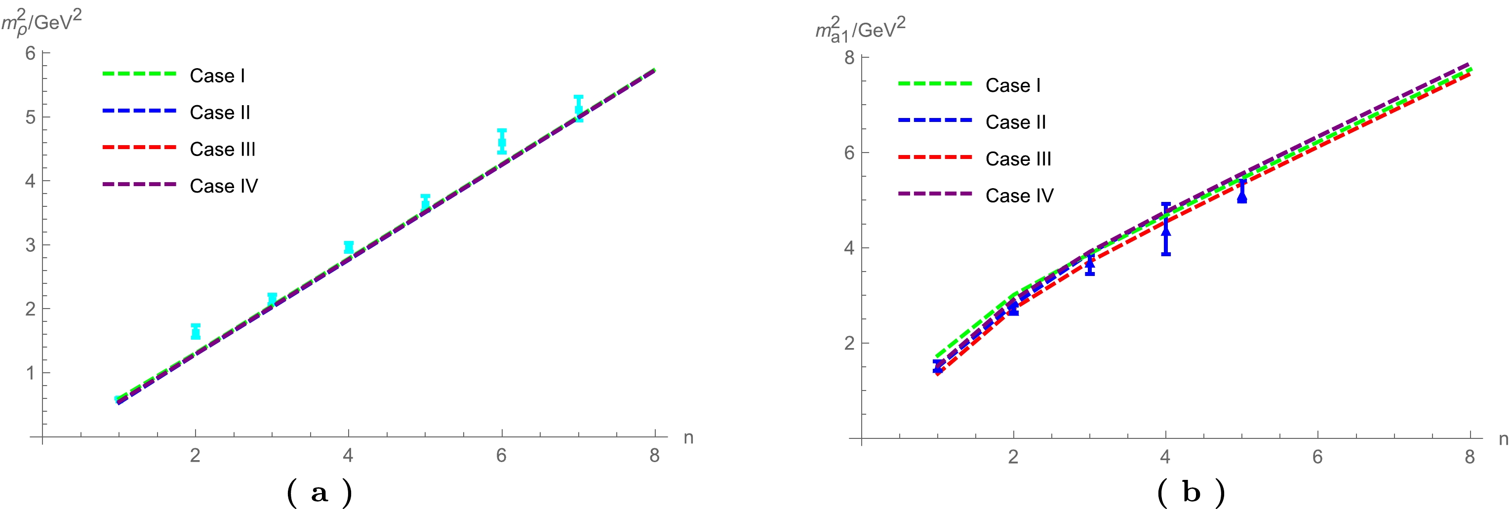
Figure 4. (color online) Spectra of vector (a) and axial vector mesons (b). Case-I: Model-IB with
$ \gamma=0 $ , Case-II: Model-IB with model$ \gamma(z) $ taking the form of$\gamma(z)=-\dfrac{3}{2}({\rm e}^{-\Phi^2/2}-1)$ , Case-III: Model-IB with dynamical$ \gamma(z) $ solving from running coupling, and Case-IV: Model IB with a constant$ \gamma=0.45 $ . The cyan and blue dots are experimental data, taken from Ref. [42], with a selection scenario following Ref. [14].For the lower excitations of axial vector mesons, the corrections of the anomalous dimension reduce the masses, and the results becomes closer to the experimental data. From Fig. 4(b), one can see that the results of Case III are significantly improved for both lower excitations and higher excitations.
-
Using the formulae in Sec. IV, we can study the anomalous dimension corrections to the form factors and the decay constants. We present the results for the decay constants and effective couplings in Table 5 and plot the results for the form factors in Fig. 5. In Table 5, we see that with the anomalous dimension corrections, the decay constant of pions (ρ), i.e.,
$ a_1 $ , decreases. However, the result for the effective coupling$ g_{\rho\pi\pi} $ in Case III is closer to the experimental value. The pion form factor$ F_\pi(Q^2) $ has been investigated in light-front holographic QCD [43], and it was found to be in good agrreement with experimental data.Exp./MeV Case-I/MeV Case-II/MeV Case-III/MeV Case-IV/MeV $ f_\pi $ 

$ 92.4\pm0.35 $ 

83.6 81.0 70.8 80.3 $ F_\rho^{1/2} $ 

$ 346.2\pm1.4 $ 

282 267 273 273 $ F_{a_1}^{1/2} $ 

$ 433\pm13 $ 

452 409 406 422 $ g_{\rho\pi\pi} $ 

$ 6.03\pm0.07 $ 

3.14 3.02 3.77 3.11 Table 5. Decay constants and couplings for different models. Case-I: Model-IB with
$ \gamma=0 $ , Case-II: Model-IB with model$ \gamma(z) $ taking the form of$\gamma(z)=-\dfrac{3}{2}({\rm e}^{-\Phi^2/2}-1)$ , Case-III: Model-IB with dynamical$ \gamma(z) $ solving from running coupling, and Case-IV: Model IB with a constant$ \gamma=0.45 $ .
Figure 5. (color online) Form factor
$ F_\pi $ as a function of$ Q^2 $ for different models. Case-I: Model-IB with$ \gamma=0 $ , Case-II: Model-IB with model$ \gamma(z) $ taking the form of$\gamma(z)=-\dfrac{3}{2}({\rm e}^{-\Phi^2/2}-1)$ , Case-III: Model-IB with dynamical$ \gamma(z) $ solving from running coupling, and Case-IV: Model IB with a constant$ \gamma=0.45 $ . -
In this work, we introduce the anomalous dimension of the scalar operator
$ \bar{q}q $ in the dynamical holographic model and study its corrections to the meson spectra, the decay constants, and the pion form factor. It is shown that with the anomalous dimension corrections, the background metric and the scalar field receive significant corrections, especially in the IR region. The scalar meson spectrum is significantly improved, especially for the low lying states. The vector meson spectra are almost unaffected by the anomalous dimension of the scalar operator$ \bar{q}q $ . Only the ground state of the vector meson receives a correction within$7$ %. When the anomalous dimensions are added, the properties of the vacuum receive corrections. Correspondingly, the interactions between the strong interacting partons also receive corrections. From our numerical calculation, as shown in Fig. 6, the interactions in the short range ($ z\rightarrow0 $ ) and long range ($ z\rightarrow \infty $ ), which are controlled by the perturbative physics (Coulomb-like$ \sim 1/z^2 $ ) and the confinement physics ($ \sim z^2 $ ), respectively, are almost unaffected by the anomalous dimension, whereas in the intermediate region, the potentials receive significant corrections. For the scalar channel, considering the anomalous dimension, the interaction energy in the intermediate region increases (in some sense, the interaction becomes more "repulsive"), while that for the vector channel becomes more "attractive." Therefore, the low lying scalar meson becomes heavier, while the vector meson becomes lighter. Because the anomalous dimension significantly affects the background metric and fields, the masses of pions and the axial vector mesons also receive important corrections, especially for the low lying states. In summary, the introduction of the anomalous dimension can improve the description of light mesons, especially for the scalar meson. In the current work, we only consider the anomalous dimension of the scalar operator. It would also be interesting to consider the corrections from other operators; we leave this for future research.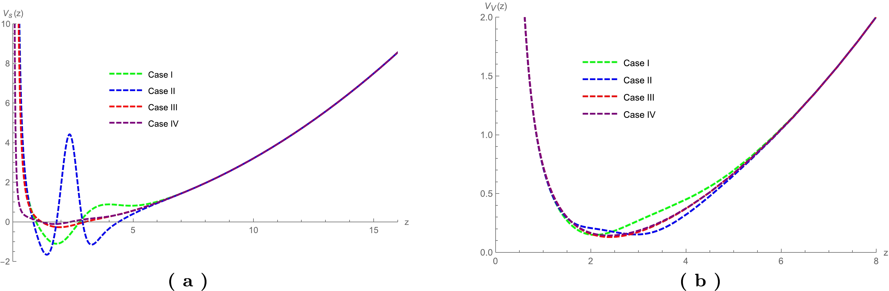
Figure 6. (color online) The Schrödinger-like potentials for scalar mesons (a) and vector mesons (b).
-
Generally, the masses (m) of hadrons can be extracted from the poles of the corresponding correlation functions, which take the form of
$ G(p^2)\propto \dfrac{1}{p^2-m^2} $ with the momentum$ p^2 $ near the poles. Therefore, one can solve the correlation functions and obtain the masses from their poles. This is the standard method based on 4D field theory. As shown in [11], in the holographic description, the solution of the poles can also be obtained by solving the egienvalues of the Schrödinger-like equations. In this appendix, we show the relation between the poles of the correlation functions and the egienvalues of the Schrodinger-like equation.Here, we take the vector sector as an example. A basic assumption is that the 5D vector field
$ V_\mu^a $ is dual to the 4D operator$ \bar{\psi}\gamma_\mu\tau^a\psi $ . To acquire the correlation functions, one needs to obtain the partition function$ Z[j_\mu(x)] $ with respect to the source$ j_\mu^a $ (we ignore the$S U(2)$ index a in the following part because it is irrelevant to the poles). From the dictionary, one can obtain the 4D correlation function from the 5D one, and it has the form$Z[j(x)]={\rm e}^{{\rm i}S_{\rm onshell}[V(z=0,x)=j_\mu(x)]}$ , where the saddle point approximation is applied. Then, the main task is to obtain the onshell action$S_{\rm onshell}$ under the condition$ V_\mu(z=0,x)=j_\mu(x) $ .With the metric ansatz Eq. (7), one can easily derive the equation of motion for the vector field as
$ \partial_z[{\rm e}^{A_s-\Phi}\partial_z V_\mu(z,x)]+\partial_\nu\partial^\nu V_\mu(z,x)=0, \tag{A1} $

and the onshell action is derived as
$ S=-\frac{1}{2g_5^2}\int {\rm d}z {\rm d}^4x\partial_z\big( {\rm e}^{3A_s-\Phi}V_\mu\partial_zV^{\mu}\big),\tag{A2} $

where we have inserted the equation of motion into the action. We can transform the 5D field
$ V_\mu $ to the momentum space$V_\mu(z,x)\simeq\int {\rm d}^4q \tilde{V}_\mu(z,q) {\rm e}^{{\rm i} q_\mu x^\mu}$ . Then, the expressions for the EOM and the on-shell action become$ \partial_z[{\rm e}^{A_s-\Phi}\partial_z \tilde{V}_\mu(z,q)]+q^2 {\rm e}^{A_s-\Phi} \tilde{V}_\mu(z,q)=0, \tag{A3} $

$ S^{\rm onshell}=-\frac{1}{2g_5^2}\int {\rm d} z {\rm d} ^4q\partial_z\big( {\rm e}^{3A_s-\Phi}\tilde{V}_\mu(z,-q)\partial_z\tilde{V}^{\mu}(z,q)\big). \tag{A4} $

According to the dictionary, we can take
$ \tilde{V}^{\mu}= V(z,q)j^{\mu}(q) $ , with j the 4D source depending on the 4D momentum$ q^\mu $ only and$ V(z,q) $ representing the z dependent part of$ V^{\mu} $ . Then, it is easy to see that$ V(z,q) $ satisfies$ \partial_z[{\rm e}^{A_s-\Phi}\partial_z V(z,q)]+q^2 {\rm e}^{A_s-\Phi} V(z,q)=0. \tag{A5} $

The onshell action then becomes
$ S^{\rm onshell}=-\frac{1}{2g_5^2}\int {\rm d} z {\rm d}^4q\partial_z\big( {\rm e}^{A_s-\Phi}V\partial_z V\big)j_\mu j^\mu.\tag{A6}$

In order to ensure that the partition function depends on the 4D boundary quantities only, one has to impose an additional boundary condition at
$ z=\infty $ , i.e.,${\rm e}^{A_s-\Phi}V\partial_zV|_{z=\infty}=0$ . Following [11], we take$ \partial_zV|_{z=\infty}=0 $ . Thus, we can integrate over the z direction and obtain$ S^{\rm onshell}=-\frac{1}{2g_5^2}\int {\rm d}^4q j_\mu j^\mu\big( {\rm e}^{A_s-\Phi}V\partial_z V\big)|_{z=\epsilon}. \tag{A7}$

In the asymptotic AdS region,
$ A(z)\simeq -\ln(z) $ , and we can obtain the near boundary condition of$ V(z) $ as$ V(z,q)\rightarrow v_0(q)+v_2(q)z^2+... \; \; \; . \tag{A8} $

Here, we have omitted the higher powers of z. Considering that at the boundary
$ z=0 $ , we have$ V^\mu(z,q)=j^\mu(q) $ , we have$ V(z=0)=1 $ . We can normalize the solution with$ v_0(q) $ . By inserting it into the on-shell action, one obtains$ S^{\rm onshell}\simeq-\frac{1}{2g_5^2}\int {\rm d}^4q j_\mu^a(-q) j^{a,\mu}(q) \frac{v_2(q)}{v_0(q)}. \tag{A9} $

It is not difficult to see that the correlation function is proportional to
$ G(q)\propto \frac{v_2(q)}{v_0(q)}. \tag{A10}$

Here, we show the part relevant to the poles only. From this expression, the poles
$ q_n^2\equiv m_n^2 $ satisfy$ v_0(q=q_n)=0 $ .Up to now, we have seen that, to obtain the poles, one does not need the full form of the correlation function. Instead, one can seek the solution of the masses
$ q_n^2 $ , which gives a solution satisfying Eq. (A5) and the boundary conditions$ V(z=0,q_n)=v_0=0 $ ,$ (V\partial_zV)|_{z=\infty}=0 $ .Then, we can use another familiar form to obtain the poles
$ q_n^2 $ or$ m_n^2 $ . In Eq. (A5), we can do a transformation$ V(z)={\rm e}^{\frac{A_s-\Phi}{2}}\psi(z). \tag{A11} $

Then, Eq. (A5) becomes
$ -\psi^{\prime\prime}(z)+V_{\rm eff}(z)=q^2\psi(z), \tag{A12} $

$ V_{\rm eff}(z)=\Bigg(\frac{A_s^\prime-\Phi^\prime}{2}\Bigg)^2+\frac{A_s^{\prime\prime}-\Phi^{\prime\prime}}{2}. \tag{A13}$

To obtain the poles, we should impose
$V(z=0)={\rm e}^{A_s-\Phi} \psi(0)= \dfrac{\psi(z)}{z}|_{z=0}=0$ , and$\partial_zV|_{z=\infty}=\partial_z({\rm e}^{-(A_s-\Phi)/2}\psi(z))|_{z=\infty} =0$ . Actually, they are equivalent to the form used in many references:$ \psi(z=0)=\psi^\prime(z=\infty)=0 $ . Then, if we solve the above Schrödinger-like equation under these boundary conditions, we can obtain the same poles that are acquired by solving Eq. (A5). For the other sectors, the derivation of the equivalence of the two methods is similar; we do not repeat it here (for the scalar sector, one can refer to [44, 45]).
Hadron spectra and pion form factor in dynamical holographic QCD model with anomalous 5D mass of scalar field
- Received Date: 2023-01-17
- Available Online: 2023-06-15
Abstract: The simplest version of the dynamical holographic QCD model is described by adding the KKSS model action on a dilaton-graviton coupled background, in which the AdS


 DownLoad: