


 Abstract
 HTML
HTML Reference
 Related
 PDF
PDF


-
In quantum chromodynamics (QCD), gluons carry color charges and have a direct strong interaction among themselves. Therefore, it is expected that hadrons can be made up of gluons solely, namely glueballs. The property of glueballs has been one of the most prominent topics in hadron physics for several decades and has been the focus of extensive and intensive experimental and theoretical studies. However, their existence has not yet been confirmed.
Glueballs are well defined objects in the quenched approximation where the quark-gluon transitions are switched off, and in quenched lattice QCD (QLQCD) studies, the existence of purge gauge glueballs has been confirmed, and their spectrum has been predicted [1, 2]. In the presence of dynamical quarks, the situation is more complicated owing to the decays of glueballs and the possible mixing between glueballs and
$ q\bar{q} $ mesons. There have been a few preliminary full-QCD lattice studies [3–5] at pion masses much larger than the physical value, in which possible glueball states with masses close to the predictions from QLQCD were observed. However, it is still challenging to verify the previous glueball studies at the physical pion mass because of the computational cost, as glueball related lattice studies usually require large statistics of thousands of gauge configurations, which is computationally prohibitive for physical pion masses and large spatial volumes at the present stage. Fortunately, the cluster decomposition principle ensures that the correlation length between the glueball operators is insensitive to the volume and can be implemented to reduce the statistical errors of glueball correlation functions. In Refs. [6–8], a cluster decomposition error reduction (CDER) method was introduced to suppress the statistics requirement on lattices with large spatial volumes. In this work, we use the CDER method to trade the statistical uncertainty for a negligible systematic one and obtain the clear mass spectrum and Bethe-Salpeter wave function with the pure glueball operators on only$ \sim $ 300 configurations at the physical pion mass. -
We choose two RBC/UKQCD gauge ensembles (labeled as 48I and 64I) with a
$ 2+1 $ flavor domain wall fermion at physical pion and kaon masses and with spatial sizes around$ 5.5 $ fm. The parameters of the ensembles are shown in Table 1 of Ref. [9]. To extract glueball states, we adopt the strategy used in Ref. [1, 2] to build the glueball operator set$ \mathcal{S}(R^{PC})=\{\mathcal{O}_\alpha, \alpha= 1,2,\ldots, 24\} $ for the scalar ($ R^{PC}=A_1^{++} $ ), pseudoscalar ($ A_1^{-+} $ ), and tensor ($ E^{++}\oplus T_2^{++} $ ) channels, where$ R=A_1, E, T_2 $ are the irreducible representations (irrep) of the lattice symmetry group O, and P and C are the parity and the charge conjugate quantum numbers, respectively.$ L^3\times T $ 

$a^{-1}\;{\rm{ /GeV} }$ 

$m_\pi\;{\rm{ /MeV} }$ 

$La \;{\rm{ /fm} }$ 

$ N_\mathrm{conf} $ 

$ 48^3\times\ \ 96 $ 

1.730(4) $ 139.2(4) $ 

$ 5.476(12) $ 

364 $ 64^3 \times 128 $ 

2.359(7) $ 139.2(5) $ 

$ 5.354(16) $ 

300 Table 1. Parameters of the 48I and 64I ensembles [9].
-
It is well known that the glueball relevant lattice study usually requires large statistics, but we have only
$ N_\mathrm{conf}\sim 300 $ configurations available for the two ensembles. Fortunately, their large lattice sizes make the cluster decomposition error reduction method (CDER) [7] feasible for improving the signal-to-noise ratio in the calculation. The idea of CDER is as follows: because$ \mathcal{C}_{\alpha\beta}(\mathbf{r},t)\equiv \langle 0|\mathcal{O}_\alpha(\mathbf{r},t)\mathcal{O}_\beta(\mathbf{0},0)|0\rangle $ behaves as$ \begin{equation} \mathcal{C}_{\alpha\beta}(\mathbf{r},t)\sim \xi^{-\frac32} {\rm e}^{-m\xi}\; \; (\xi\to \infty), \end{equation} $

(1) where m represents the lowest mass in this channel and
$ \xi=(\mathbf{r}^2+t^2)^{1/2} $ represents the Euclidean separation between the sink and the source operator, the signals of$ \mathcal{C}_{\alpha\beta} $ will be undermined by statistical noise when$ |\mathbf{r}| $ is beyond some length scale$ |\mathbf{r}_c|\propto 1/m $ . Therefore, the correlation matrix$ C_{\alpha\beta} $ with the operator set$ \mathcal{S}(R^{PC}) $ for a given$ R^{PC} $ channel can be calculated as$ \begin{aligned}[b] \mathcal{C}_{\alpha\beta}(t)=&\frac{1}{T}\sum\limits_{\tau,\mathbf{x,r}} \langle 0|\mathcal{O}_\alpha(\mathbf{x+r},t+\tau)\mathcal{O}_\beta(\mathbf{x},\tau)|0\rangle\\ \simeq &\sum\limits_{|\mathbf{r}|<r_c} K_{\alpha\beta}(\mathbf{r},t)\equiv \mathcal{C}_{\alpha\beta}(r_c,t), \end{aligned} $

(2) where the average over time slices is taken into account to improve the statistics, and the kernel functions
$ K_{\alpha\beta}(\mathbf{r},t) $ are introduced as$ \begin{equation} K_{\alpha\beta}(\mathbf{r},t)=\sum\limits_{\mathbf{k}} {\rm e}^{-{\rm i}\mathbf{k}\cdot \mathbf{r}} \langle 0|\hat{\mathcal{O}}_\alpha(-\mathbf{k},t)\hat{\mathcal{O}}_\beta(\mathbf{k},t)|0\rangle \end{equation} $

(3) in terms of the Fourier transformed operators
$\hat{\mathcal{O}}_\alpha(-\mathbf{k},t)= \sum\limits_{\mathbf{x}}{\rm e}^{-{\rm i}\mathbf{k}\cdot\mathbf{x}}\mathcal{O}_\alpha(\mathbf{x},t)$ . The cutting scale parameter$ r_c $ is chosen empirically when the value of$ \mathcal{C}_{\alpha\beta}(r_c,t) $ is saturated. Note that the vacuum subtraction is necessary for$ A_1^{++} $ operators because they have the same quantum numbers as the vacuum. Before the CEDR scheme is applied, for each of the$ A_1^{++} $ operators, the vacuum subtraction is performed through the replacement$ \begin{equation} \mathcal{O}_\alpha (x)\to \mathcal{O}_\alpha(x)-\frac{1}{V}\langle \sum\limits_x \mathcal{O}_\alpha(x)\rangle, \end{equation} $

(4) where V represents the 4-D volume, and
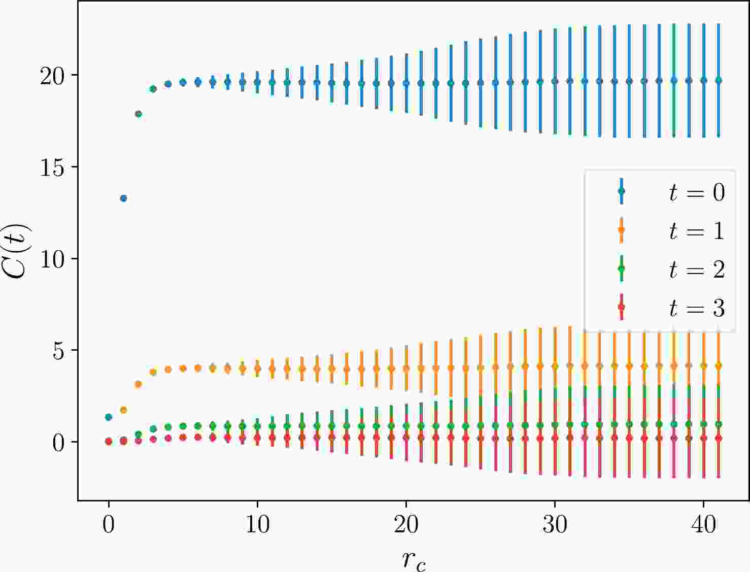
$ \langle \mathcal{O}_\alpha\rangle $ is the average of$ \mathcal{O} $ over the gauge ensemble involved. After the CDER scheme, the vacuum subtraction is successfully fulfilled. In practice, the above procedure is applied to all the considered channels.The efficacy of CDER is illustrated in Figs. 1 and 2, where a typical
$ \mathcal{C}_{\alpha\beta}(r_c, t) $ in the$ A_1^{++} $ channel at different fixed time slices is plotted versus$ r_c/a $ . One can see the central values of$ \mathcal{C}_{\alpha\beta}(r_c,t) $ at different t are saturated uniformly beyond$ r_c/a=7 $ , but the errors grow with an increase in$ r_c $ . In the practical calculation, we choose$ r_c/a=7 $ for all the$ \mathcal{C}_{\alpha\beta}(R,t) $ in all the channels.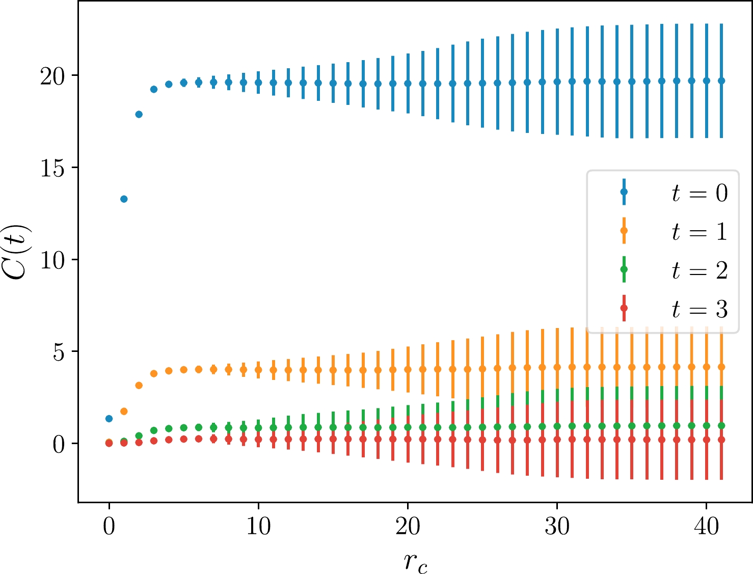
Figure 1. (color online) Plot of the
$ A_1^{++} $ correlation function at the first 4 times slices against the cutoff on the$ 48^3 \times 96 $ lattice. The$ r_c $ is in lattice unit. As expected, the signal reaches the maximum at$ r_c\sim 7a $ , and only the noise increases afterwards. Here, the error bars indicate the standard deviations instead of statistical errors.
Figure 2. (color online) Same as Fig. 1 but in logarithm scale with the standard error for larger t. One can see that the error becomes unacceptable for
$ r_c > 12a $ . We expect that reliable results can be extracted from$ r_c = 7a $ .In each
$ R^{PC} $ channel, after the correlation matrix$ \mathcal{C}_{\alpha\beta}(t) $ is estimated through Eq. (2), we perform the standard variational method by solving the generalized eigenvalue problem$ \mathcal{C}_{\alpha\beta}(t)v_\beta=\lambda(t,t_0) \mathcal{C}_{\alpha\beta}(t_0)v_\beta $ . In practice, we use$ t_0=0 $ and$ t=a $ . The eigenvector$ v_\alpha^{(n)} $ of the n-th largest eigenvalue gives an optimized operator$ \mathcal{O}_n= v_\alpha^{(n)}\mathcal{O}_\alpha $ that is expected to couple most to the n-th lowest state$ |n\rangle $ . In other words, the correlation function$ \mathcal{C}_n(t) $ of$ \mathcal{O}_n $ behaves as$ \begin{equation} \mathcal{C}_n(t)=\langle 0|\mathcal{O}_n(t) \mathcal{O}_n(0)|0\rangle\sim {\rm e}^{-m_n t}, \end{equation} $

(5) where the eigenvectors
$ v_\alpha^{(n)} $ are normalized by requiring$ \mathcal{C}_n(0)=1 $ . This implies that$ \langle 0|\mathcal{O}_n|m\rangle \approx \delta_{mn} $ if the states are normalized as$ \langle m|n\rangle=\delta_{mn} $ .Although the operator basis in each channel is large, it is found that the correlation function of the operator
$ \mathcal{O}_1 $ optimized for the ground state still has a sizeable contribution from other states; namely, the effective mass function does not show a good enough plateau in the early time range (especially in the$ E^{++} $ channel), as shown in Fig. 3. In order to enhance the contribution of the ground state to the corresponding correlation functions, we construct another type of gluonic operator in terms of the gauge potential$ A_\mu(x) $ [10, 11] in the Coulomb gauge.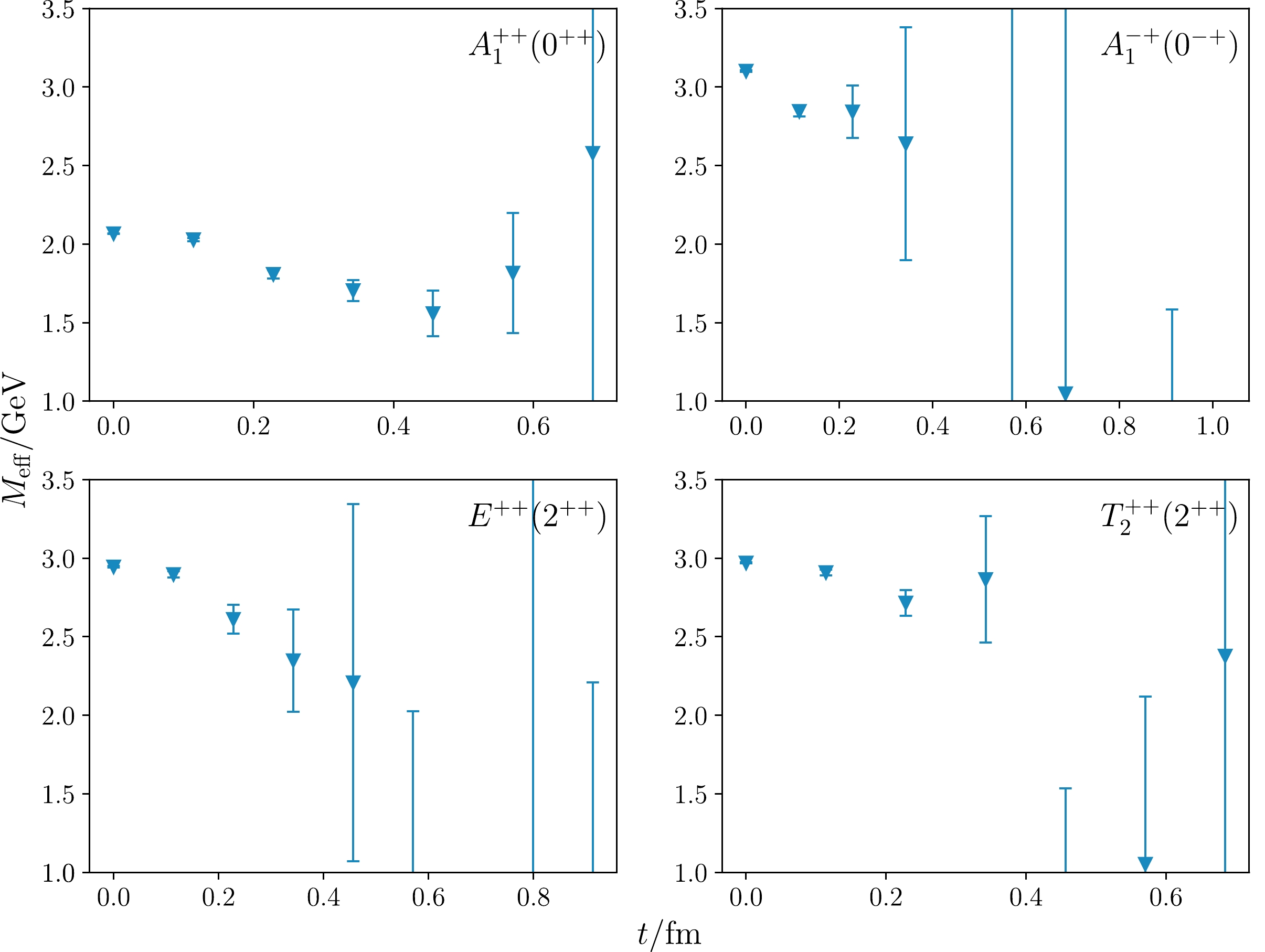
Figure 3. (color online) The effective mass plots of the correlation functions
$ \mathcal{C}_1(t) $ in Eq. (5) for$ A_1^{++} $ ,$ E^{++} $ ,$ T_2^{++} $ , and$ A_1^{-+} $ channels on 48I. -
According to the definition of the gauge link oriented in the μ direction starting from the lattice site, i.e.,
$U_\mu(x)= \exp[-{\rm i}agA_\mu(x)]$ , up to an irrelevant pre-factor, we have$ \begin{equation} A_\mu(x) \equiv {\rm i}\, {\mathrm{ln}} U_\mu(x) \end{equation} $

(6) where
$ {\mathrm{ln}} U_\mu(x) $ can be derived as${\mathrm{ln}} U_\mu(x)= V(x) {\mathrm{diag}} ({\mathrm{ln}} \lambda_1(x), ~ {\mathrm{ln}} \lambda_2(x),~ {\mathrm{ln}}\lambda_3(x)) V^\dagger(x)$ with$ \lambda_{1,2,3}(x) $ being the eigenvalues of$ U_\mu(x) $ and$ V(x) $ being the unitary matrix that diagonalizes$ U_\mu(x) $ . The properties of$U_\mu(x)\in S U(3)$ require$ \lambda_1\cdot\lambda_2\cdot\lambda_3=1 $ and$ |\lambda_{1,2,3}|=1 $ , such that$ \lambda_{1,2,3} $ can be expressed as$\lambda_i={\rm e}^{{\rm i}\theta_i}\; (i=1,2,3)$ with$ \theta_i\in [-\pi,\pi) $ .On each time slice, the spatially extended operator
$ \mathcal{O}_A^R(r,t) $ can be constructed by$ A_\mu(x) $ at two different points. For$ P=C=+ $ , the explicit expression of$ \mathcal{O}_A^R(r,t) $ of the quantum number$ R^{PC} $ is$ \begin{equation} \mathcal{O}_A^R(\mathbf{x},t;r)=\frac{1}{N_r} \sum\limits_{ij,|\mathbf{r}|=r} {\mathrm{tr}} S_{ij}^R[A_i(\mathbf{x+r})A_j(\mathbf{x})], \end{equation} $

(7) where
$ N_r $ is the degeneracy of$ \mathbf{r} $ with the same r and$ S_{ij}^R $ are the combinational coefficients related to the irrep R of the spatial symmetry group O (octahedral group) on the lattice. For$ R=A_1, E, T_2 $ , the non-zero values of$ S_{ij}^R $ are as follows:$ \begin{aligned}[b] S_{11}^{A_1}=&S_{22}^{A_1}=S_{33}^{A_1}=1\\ S_{11}^{E,1}=&-S_{22}^{E,1}=\frac{1}{\sqrt{2}}\\ S_{11}^{E,2}=&S_{22}^{E,2}=-\frac{1}{\sqrt{6}}, \; \; S_{33}^{E,2}=\frac{2}{\sqrt{6}}\\ S_{jk}^{T_2,i}=& |\epsilon_{ijk}|,\; \; i,j,k=1,2,3. \end{aligned} $

(8) The
$ O_A^R(r,t) $ operator for$ A_1^{-+} $ is defined as$ \begin{equation} \mathcal{O}_A^{A_1^{-+}}(\mathbf{x},t;r)=\frac{1}{N_r}\sum\limits_{|\mathbf{r}| = r} \epsilon_{ijk} {\mathrm{tr}}\left[A_i(\mathbf{x} + \mathbf{r}) A_j(\mathbf{x})\right] \hat r_k \,, \end{equation} $

(9) where
$ \hat{\mathbf{r}} $ is the orientation vector of$ \mathbf{r} $ .In each channel, through the implementation of CDER similar to Eqs. (2) and (3) and using the same
$ r_c=7a $ , we calculate the correlation function$ \mathcal{C}_{An}(r,t) $ of$ O_A^R $ and the n-th optimized operator$ \mathcal{O}_n $ :$ \begin{aligned}[b] \mathcal{C}_{An}(r,t)=&\frac{1}{T}\sum\limits_{\tau,\mathbf{x,y}} \langle 0|\mathcal{O}_A^R(\mathbf{x},t+\tau;r)\mathcal{O}_n(\mathbf{y},\tau)|0\rangle\\ \approx& \Phi_n(r){\rm e}^{-m_n t}+\sum\limits_{i\ne n}\epsilon_m \Phi_m(r){\rm e}^{-m_i t}, \end{aligned} $

(10) where the last parametrization is due to predominant coupling of
$ \mathcal{O}_n $ to the n-th state with$ \epsilon_i \ll 1 $ , and$ \Phi_n(r)\propto \langle 0|\mathcal{O}_A^R(\mathbf{0},t;r)|n\rangle $ is interpreted as the Bethe-Salpeter (BS) wave function [12] of the n-th state$ |n\rangle $ if it is a two-gluon glueball state. In principle,$ \Phi_n(r) $ can be approximated by$ \mathcal{C}_{An}(r,t) $ at any t according to Eq. (10). However, owing to the rapid increase in the noise, we can only observe clear signals of$ \Phi_n(r) $ at the first few time slices. Figure 4 shows the profiles of$ \Phi_{1,2}(r) $ at$ t=0 $ for$ A_1^{++} $ ,$ A_1^{-+} $ ,$ E^{++} $ , and$ T_2^{++} $ channels on 48I and 64I lattices (normalized by$ \Phi(r=0) = 1 $ for$ PC=++ $ channels and$ \Phi(r=a)=1 $ for the$ A_1^{-+} $ channel), where the values of r are converted into physical units using the lattice spacings a in Table 1. Similar to that in Refs. [10, 11], the data points of$ \Phi_n(r) $ can be described by some phenomenological functional forms. For the ground state and first exited state of$ A_1^{++} $ ,$ E^{++} $ , and$ T_2^{++} $ , the functions take the forms
Figure 4. (color online) Normalized BS wave functions of the ground and first excited states on the 48I and 64I lattices.
$ \begin{aligned}[b] \Phi_1(r) & = A {\rm e}^{-(r / r_0)^\alpha}+D \\ \Phi_2(r) & = A (1 - \beta r^\alpha) {\rm e}^{-(r / r_0)^\alpha}+D'. \end{aligned} $

(11) For
$ A_1^{-+} $ , the corresponding function forms are$ \begin{aligned}[b] \Phi_1(r) & = A r {\rm e}^{-(r / r_0)^\alpha}+D \\ \Phi_2(r) & = A r (1 - \beta r^\alpha) {\rm e}^{-(r / r_0)^\alpha}+D'. \end{aligned} $

(12) In the functions forms above, the constants D and
$ D' $ are added to account for the possible contamination from the unphysical modes of domain-wall sea quarks, as will be explained in a later section. By using these functions forms to fit$ C_{An}(r,t=0) $ in each channel, we obtain the parameters$\alpha,~\beta,~ r_0$ , whose best-fit values are given in Table 2. These functions with the fitted parameters are also plotted in Fig. 4 as curves. It is seen that the functions describe the data points fairly well. It is interesting that the r-behaviors of$ \Phi_{1,2}(r) $ in$ PC=++ $ channels are very similar to the radial$ 1S $ and$ 2S $ Schrödinger wave function of a two-body system with a central potential. These behaviors and the parameters α and$ r_0 $ are very similar to those obtained in the quenched approximation [11]. The BS wave functions in the$ A_1^{-+} $ channel are derived for the first time on the lattice and have the feature of$ 1P $ and$ 2P $ wave functions. Note that, by solving the Bethe-Salpeter equation of the$ 0^{-+} $ glueball, the two-body P-wave feature of the$ 0^{-+} $ Bethe-Salpeter amplitude was also observed in Refs. [13–15].$ R^{PC} $ 

n $ r_0 $ /fm

α β 48I $ A_1^{++} $ 

1 $ 0.14(4) $ 

$ 1.6(2) $ 

2 $ 0.16(5) $ 

$ 1.5(2) $ 

$ 24(1) $ 

$ E^{++} $ 

1 $ 0.24(7) $ 

$ 1.8(2) $ 

2 $ 0.22(5) $ 

$ 1.6(2) $ 

$ 16(1) $ 

$ T_2^{++} $ 

1 $ 0.26(9) $ 

$ 2.0(3) $ 

2 $ 0.25(8) $ 

$ 1.8(3) $ 

$ 19(2) $ 

$ A_1^{-+} $ 

1 $ 0.24(8) $ 

$ 1.9(3) $ 

2 $ 0.23(7) $ 

$ 1.8(3) $ 

$ 12(1) $ 

64I $ A_1^{++} $ 

1 $ 0.15(3) $ 

$ 1.4(1) $ 

2 $ 0.20(10) $ 

$ 1.5(4) $ 

$ 18(2) $ 

$ E^{++} $ 

1 $ 0.24(6) $ 

$ 1.7(2) $ 

2 $ 0.22(8) $ 

$ 1.7(3) $ 

$ 17(2) $ 

$ T_2^{++} $ 

1 $ 0.26(6) $ 

$ 1.9(2) $ 

2 $ 0.23(5) $ 

$ 1.8(2) $ 

$ 18(1) $ 

$ A_1^{-+} $ 

1 $ 0.20(5) $ 

$ 1.7(2) $ 

2 $ 0.19(6) $ 

$ 1.6(2) $ 

$ 10(1) $ 

Table 2. Fitted parameters of Bethe-Salpeter wave function form in Eqs. (11) and (12).
We would not like to put too much emphasis on the interpretation of the wave functions
$ \Phi_n(r) $ but will use the feature of the r-behaviors of these functions to enhance the contribution of the ground states in the early time region. Because$ \Phi_2(r) $ in each channel has a radial node at$ r=r_1 $ , the correlation function$ \mathcal{C}_{A1}(r_1,t) $ in each channel is expected to be dominated by the ground state, as the second term in Eq. (10) is further suppressed by$ \Phi_2(r_1)\approx 0 $ . According to Fig. 4, the radial node of$ \Phi_2(r) $ appears at$r\sim 0.12,~ 0.19$ and 0.22 fm in the scalar ($ A_1^{++} $ ), the tensor ($ E^{++} $ and$ T_2^{++} $ ), and the pseudoscalar channel ($ A_1^{-+} $ ), respectively. According to the lattice spacings in Table 1, we choose$ r_1(A_1^{++})/a=\sqrt 2 $ ,$ r_1(E^{++}, T_2^{++})/a=\sqrt{3} $ , and$ r_1(A_1^{-+})/a=2 $ on the 48I lattice. On the 64I lattice, these$ r_1/a $ 's are chosen to be$ \sqrt{5} $ ,$ \sqrt{5} $ , and$ 2\sqrt{2} $ . At these values of$ r_1 $ , the$ \Phi_2(r) $ values are seen to be approximately zero. The effective mass of each$ \mathcal{C}_{An}(r_1,t) $ for all four channels on the two ensembles (48I and 64I) are illustrated in Fig. 5, where the vertical axis and the horizontal axis are plotted in physical units. It is seen that the effective masses show more or less plateaus at the first several time slices, which indicates that$ C_{A1}(r_1,t) $ can be described with a single exponential, as expected.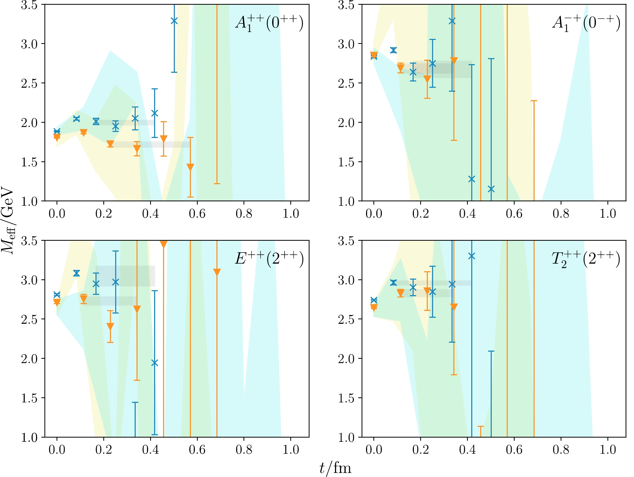
Figure 5. (color online) Effective masses of
$ C_{A1}(r_1,t) $ on 48I (orange triangles) and 64I (blue crosses), with the shaded region showing the results obtained without CDER. The gray bands show the fitting results and fitting windows obtained through single-exponential function forms.With the prescription mentioned above, the ground state masses in each channel are extracted through single exponential function forms in early time windows. In each panel of Fig. 5, the grey bands illustrate the fitting results and the time intervals of the fits. In order to exhibit the efficacy of the CDER method, we also show the lattice data that are derived by calculating the correlation functions without the implementation of CDER in green (48I ensemble) and yellow bands (64I ensemble). Obviously, the data without CDER fluctuate drastically with respect to time, and the errors are quite large. In contrast, the data points based on the CDER method have much smaller errors at the first 4-6 time slices and show more or less plateaus. From the plateau regions indicated by the grey bands in Fig. 5, we obtain estimates of the ground state mass values, which are listed in Table 3 in physical units. We make the following observations:
$\mathrm{ensemble}$ 

$ m(A_1^{++}) $ 

$ m(E^{++}) $ 

$ m(T_2^{++}) $ 

$ m(A_1^{-+}) $ 

48I $ 1.718(34) $ 

$ 2.729(54) $ 

$ 2.829(46) $ 

$ 2.685(60) $ 

$ \chi^2 / \mathrm{dof} $ 

0.76 0.82 0.01 0.12 64I $ 1.995(30) $ 

$ 3.05(13) $ 

$ 2.958(28) $ 

$ 2.67(10) $ 

$ \chi^2 / \mathrm{dof} $ 

0.18 1.95 0.09 0.22 Table 3. Fitted masses of the ground states in
$ A_1^{++}, E^{++}, $ $ T_2^{++}, A_1^{-+} $ channels on 48I and 64I ensembles. The masses are converted into values in physical units (GeV) using the lattice spacings in Table 1.● Given the small errors at the first several time slices, the data points do not behave very regularly but fluctuate slightly. For each channel, the effective masses from both ensembles are very close at
$ t=0 $ but become more different when t increases. A possible reason for this behavior is the contamination of oscillatory modes of the domain wall sea quarks (see below). Anyway, given the large errors, the fitted ground state masses on the$48{\rm I}$ and$64{\rm I}$ ensembles are compatible with each other except for the$ A_1^{++} $ channel.● The masses of ground states in
$ E^{++} $ and$ T_2^{++} $ channels are compatible with each other on the same ensemble. This also indicates that the discretization effects are not important, because these states correspond to the$ 2^{++} $ state in the continuum limit.● Their masses are higher than but not far from those of the quenched approximation predictions and preliminary full-QCD calculations [1–5].
The fluctuating data points of the effective masses and the constant terms in (11) and (12) may be attributed to the contamination of unphyiscal oscillatory modes of the domain wall fermions [16–18]. In the mean field approximation, the lowest unphysical mode of domain wall fermions propagates along time as
${\rm e}^{-E t}\sim(-)^{t/a} {\rm e}^{-|E_0|t}$ , with$ E_0 $ being expressed as$ \begin{equation} E_0=\frac{1}{a}{\mathrm{ln}} \left|\frac{4-M_5-3u_0}{u_0}\right|, \end{equation} $

(13) where
$ M_5 $ is the domain-wall mass parameter and$ u_0 $ is the tadpole parameter of gauge links. These modes may contribute to correlation functions of gluonic operators through the vacuum polarization of a pair of (physical and unphysical) a quark and antiquark. According to the discussion in the reference mentioned above, the energy of the unphysical fermion mode is estimated as$ |E_0| a\sim 0.716 $ for the 48I ensemble ($ M_5=1.8 $ ,$ u_0=0.876 $ ) and$ |E_0| a \sim 0.660 $ for the 64I ensemble ($ M_5=1.8 $ ,$ u_0=0.886 $ ). Using the lattice spacing$ a^{-1}\approx 1.734 $ GeV for 48I and$ a^{-1}\approx 2.360 $ GeV for 64I, the lowest energy of the excitation of a physical quark and an unphysical quark from the vacuum can be as low as roughly$ m_2\sim 1.24 $ GeV for 48I and$ 1.56 $ GeV for 64I, respectivley, both of which are lower than the expected$ 0^{++} $ glueball mass and worrisome in the data analysis of the correlation functions of gluonic operators.As indicated by the BS amplitudes shown in Fig. 4, the contributions from glueball states are expected to be highly suppressed in comparison with the
$ r=0 $ case. Thus, we check the effective mass of$ \mathcal{C}_{n1}(r,t) $ at a large r in the$ A_1^{++} $ channel, to enhance the contribution from the oscillatory modes. Figure 6 shows the effective masses of$ \mathcal{C}_{A1}(r,t) $ in the$ A_1^{++} (0^{++}) $ channel at$ r\approx 0.6 $ fm (where the glueball contribution is expected to be roughly 10 times smaller than that at$ r=0 $ according to the BS wave function). Here, the orange and blue points refer to those from the$48{\rm I}$ and$64{\rm I}$ ensembles, respectively. At the early time slices, the data points oscillate up and down. The magnitude increases with time and can be understood through the following expression:
Figure 6. (color online) Effective masses of
$ C_{A1}(0.6\; \mathrm{fm},t) $ on 48I (orange triangles) and 64I (blue crosses), where the glueball contribution is suppressed and then the oscillatory behavior is more obvious than that in Fig. 5.$ \begin{aligned}[b] m_\mathrm{eff}(t)=&\frac{1}{a}{\mathrm{ln}} \frac{C(t)}{C(t+a)}\\ =&m_1+\frac{1}{a}{\mathrm{ln}}\frac{1+(-)^{t/a} B{\rm e}^{-\Delta t}}{1+(-)^{t/a+1} B{\rm e}^{-\Delta (t+a)}}\\ &_{\overrightarrow{|B|\ll 1}} m_1+\frac{B}{a} \left(1+{\rm e}^{-\Delta a}\right)(-)^{t/a} {\rm e}^{-\Delta t}, \end{aligned} $

(14) where the correlation function
$C(t)=A {\rm e}^{-m_1 t} (1 + (-)^{t/a} B {\rm e}^{-\Delta t})$ includes both the physical states (glueballs, first term) and the oscillatory modes (second term). On the 48I and 64I ensembles we used, the mass of the oscillatory modes can be even lower than the glueball mass around 1.7–2.0 GeV, which leads to$ \Delta<0 $ . Then,${\rm e}^{-\Delta t}$ increases on t; and the effect on 64I should be weaker than that on 48I. Such a prediction is consistent with the observation in Fig. 6, as the oscillation seems to be stronger at a larger t and/or lattice spacing (orange points of 48I at$ a=0.11 $ fm v.s. blue points of 64I at$ a=0.08 $ fm).The situation for glueballs is even more complicated in the presence of dynamical quarks. Experimentally, most of hadrons are observed as resonances; therefore, their decays should be taken into account. The energy levels obtained on the lattice are actually the eigen energies of the lattice Hamiltonian, and their connection with the resonances in the real world is highly nontrivial. In full QCD, glueballs can mix with
$ \bar{q}q $ and multi-hadron states. However, with the gluonic operators, the$ \bar{q}q $ states are suppressed by$ \mathcal{O}(1/N_c) $ and two meson states are suppressed by$ \mathcal{O}(1/N_c^2) $ . This is perhaps the reason why we see the effective mass plateaus in short time separation. To have a complete picture, it is essential to include quark operators in the calculation, which is beyond the scope of the present work. There is an exploratory lattice study in this direction in the scalar channel [19], but no glueball states can be identifiable unambiguously yet. In this sense, our work makes a little progress in this direction. -
An exploratory study of glueballs is performed on two
$ N_f=2+1 $ gauge ensembles with large lattice sizes and the dynamical quark masses being tuned at the physical point. The large lattice size enables us to use the CDER technique to reduce the errors of the correlation functions of glueball operators. By using the spatially extended glueball operators defined through the gauge potential$ A_\mu(x) $ in the Coulomb gauge, the Bethe-Salpeter wave functions of the scalar ($ A_1^{++}) $ , the tensor ($ E_2^{++}\oplus T_2^{++} $ ), and the pseudoscalar ($ A_1^{-+}) $ states are derived, which are similar to the features of the non-relativistic wave functions of two-body systems. Even though the physical meaning of these BS wave functions may not be clear, we can make use of their radial behaviors to further improve the ground state domination of the related correlation functions at the early time region, where the ground state masses in each channel can be extracted through single-exponential function form. If the excited state contamination is small and the couplings to$ \bar{q}q $ meson states are negligible (they can show up at very large time separation given enough statistics), the ground state masses we obained in the scalar, tensor, and pseudoscalar channels are not far from the corresponding glueball masses in the quenched approximation. In addition to the uncontrolled systematic uncertainties due to the possible mixing with$ q\bar{q} $ states and multi-hadron states, our results may suffer from the interference from the unphysical modes of domain wall fermions. A scrutinized full-QCD study should be carried out in which the$ \bar{q}q $ and multi-meson operators are included and the resonance nature of most hadrons is considered. As a noise reduction scheme, the same CDER technique can be applied to all the correlation functions involving the disconnected quark insertions. In this sense, our study represents a breakthrough for improving the signal-to-noise ratios of correlation functions involving glueball operators and paves the way to the final answer on the existence of the glueball states. -
We thank the RBC and UKQCD collaborations for providing us their DWF gauge configurations.
Glueballs at physical pion mass
- Received Date: 2023-03-06
- Available Online: 2023-06-15
Abstract: Glueballs are investigated through gluonic operators on two


 DownLoad: