


 Abstract
 HTML
HTML Reference
 Related
 PDF
PDF


-
The nuclear shell model (SM) is one of the fundamental frameworks in nuclear physics. In this model, the wave function of a many-body quantum system can be obtained by diagonalizing a shell model Hamiltonian in a given model space. Theoretically, the SM can describe various properties of nuclei throughout the mass region. However, owing to the limitation of conventional diagonalization approaches, the full SM calculations have been restricted to rather small model spaces. To tackle the many-body problem in a large model space, the large configuration space must be truncated into a small subspace so that the diagonalization can be performed on a present-day computer. Certainly, the energies obtained in the subspace are approximate eigenenergies of the Hamiltonian. Various approximate SM methods with different choices of the configuration subspaces have been developed in an attempt to make the SM approximation as good as possible [1–6].
Among these approximate methods, the variational methods, such as the VAMPIR method [4] and the variation after projection (VAP) method [5, 6], are important ones. These methods have proven to be useful in extending the SM applicability from its traditional
$ sd $ and$ pf $ model spaces to larger ones. In the variational methods, the yrast state with given quantum numbers J and M can be easily obtained by solving the variational equation [7]. However, for the first excited state with the same symmetry, the calculation is slightly more complicated. To ensure the orthogonality between the first excited state and the yrast one, Gram-Schmidt orthogonalization is usually adopted to eliminate the yrast state from the variational space, as has been done in the VAMPIR method [4]. In principle, this procedure can be generalized to higher nonyrast states, but in fact it quickly becomes rather complicated. In Ref. [8], we proposed a new algorithm in the VAP method for the calculations of nonyrast states. It is found that the yrast state and nonyrast states with given spin J can be optimized simultaneously by minimizing the sum of the energies of the m lowest calculated states,$ S_m=\displaystyle\sum\limits_{\alpha=1}^m E_{J\alpha} $ . During the variational process, the orthogonality among the calculated states is automatically fulfilled by solving the Hill-Wheeler (HW) equation.Although this algorithm avoids the complexity of the frequently used Gram-Schmidt orthogonalization, there exists an inadequacy. The VAP calculation converges when
$ S_m $ is minimized. At this minimum, the gradient of$ S_m $ is zero. However, this does not guarantee that the gradient of each energy in$ S_m $ is also zero. Consequently, the calculated energies in$ S_m $ are not at their own minima. In this sense, one may expect that the wave function of each calculated state can be further optimized individually, so that the gradient of this energy can be as close as possible to zero. Recently, we realized that such an improvement of the VAP wave function can be achieved by assigning different weights to the calculated energies. The purpose of the present work is to develop a weighted VAP method for the calculation of low-lying nonyrast states so that the VAP approximation can be further improved. Furthermore, these improved VAP wave functions are applied to the energy-variance extrapolation, which was addressed in Ref. [9], and we expect that this may reduce the gaps between the approximate energies and the exact SM ones.The remainder of this paper is organized as follows. Section II introduces the framework of the weighted VAP method. The energy-variance extrapolation method for the nonyrast states is discussed in Sec. III. A brief summary and outlook are presented in Sec. IV.
-
The Hamiltonian of a nuclear many-body system is invariant under a number of symmetry operations, such as rotation and reflection. Thus, a nuclear wave function should have good spin and parity. Generally, such a nuclear wave function can be constructed by adopting the techniques of angular momentum projection and parity projection. With these techniques, the nuclear wave function can be expressed as
$ |\Psi^{(n)}_{J\pi M\alpha}\rangle=\sum\limits_{i=1}^n\sum\limits_{K=-J}^Jf^{J \alpha}_{Ki}P_{MK}^{J}P^{\pi}|\Phi_i\rangle, $

(1) where
$ P_{MK}^{J} $ and$ P^{\pi} $ are the projection operators of angular momentum$ (J) $ and parity$ (\pi) $ , respectively. α is used to label the states with the same J, π, and M. n represents the number of adopted$ |\Phi_i\rangle $ reference states with good particle numbers. Here$ |\Phi_i\rangle $ is assumed to be a fully symmetry-unrestricted deformed Slater determinant (SD). One can vary$ |\Psi^{(n)}_{J\pi M\alpha}\rangle $ so that it is as close as possible to the corresponding exact shell model one. This is usually called variation after projection [7].Actually, the wave function in Eq. (1) can be further simplified. In Ref. [10], we found that for each
$ |\Phi_i\rangle $ , it is enough to pick up just one of its$ (2J+1) $ projected states to form a VAP wave function, i.e.,$ |\Psi^{(n)}_{J\pi M\alpha}(K)\rangle=\sum\limits_{i=1}^nf^{J \alpha}_{i}P_{MK}^{J}P^{\pi}|\Phi_i\rangle, $

(2) where K can be randomly chosen from
$ -J $ ,$ -J+1 $ ,$ \cdots $ ,$ J-1 $ , J. The same good approximation of Eqs. (1) and (2) can be achieved if full optimization is performed [10]. In the following, all the discussions are based on the simplified wave function in the form of Eq. (2).Given a set of
$ |\Phi_i\rangle $ states, the coefficients,$ f^{J\alpha}_{i} $ , in Eq. (2) and the corresponding energy$ \begin{array}{*{20}{l}} E^n_{J\alpha}=\langle \Psi^{(n)}_{J\pi M\alpha}(K)|\hat H |\Psi^{(n)}_{J\pi M\alpha}(K)\rangle, \end{array} $

(3) are determined by solving the following HW equation:
$ \sum\limits_{i'=1}^n\langle\Phi_i|(\hat H-E^n_{J\alpha}) P^{J}_{KK}P^{\pi}|\Phi_{i'}\rangle f^{J\alpha}_{i'}=0. $

(4) The coefficients
$ f^{J\alpha}_{i} $ should also satisfy the normalization condition:$ \sum\limits_{ii'=1}^n f^{J\alpha *}_{i} \langle\Phi_i|P^{J}_{KK}P^{\pi}|\Phi_{i'}\rangle f^{J\alpha}_{i'}=1. $

(5) By solving Eq. (4), one can obtain n approximate energies,
$ E^n_{J\alpha} $ , with$ \alpha=1,2,\cdots,n $ , and the corresponding n orthogonal wave functions,$ |\Psi^{(n)}_{J\pi M\alpha}(K)\rangle $ , if the included projected states are independent. Here, we assume$ E^n_{J1}\leq E^n_{J2}\leq\cdots \leq E^n_{Jn} $ . Clearly, the wave functions,$ |\Psi^{(n)}_{J\pi M\alpha}(K)\rangle $ , are determined by the selected reference states,$ |\Phi_i\rangle $ . Hence, the VAP calculation is essentially the process of finding a set of$ |\Phi_i\rangle $ states such that the obtained nuclear wave functions,$ |\Psi^{(n)}_{J\pi M\alpha}(K)\rangle $ , are as close as possible to the corresponding SM wave functions.Generally, for the yrast state, such optimization can be easily performed by minimizing
$ E^n_{J1} $ . However, for the nonyrast states with the same J, M, and π, the optimization is far more complicated. Traditionally, for the nonyrast state α, Gram-Schmidt orthogonalization must be first applied to ensure the orthogonality between the calculated state and all the lower ones. Such orthogonalization is rather complicated if α is large. In Ref. [8], we proposed an algorithm for calculating the nonyrast states in which the Gram-Schmidt orthogonalization is no longer necessary. It is found that the lowest m ($ m\leq n $ ) states can be optimized simultaneously by minimizing the sum of the calculated lowest projected energies:$ S_m^n=\sum\limits_{\alpha=1}^m E^n_{J\alpha}. $

(6) Such minimization of
$ S_m^n $ is ensured by the Hylleraas–Undheim–MacDonald (HUM) theorem [11, 12]. According to this algorithm, the VAP calculation converges when the gradient of$ S_m^n $ ,$ \nabla S_m^n $ , becomes zero:$ \nabla S_m^n=\sum\limits_{\alpha=1}^{m}\nabla E^n_{J\alpha}=0. $

(7) Apparently, Eq. (7) does not guarantee that each
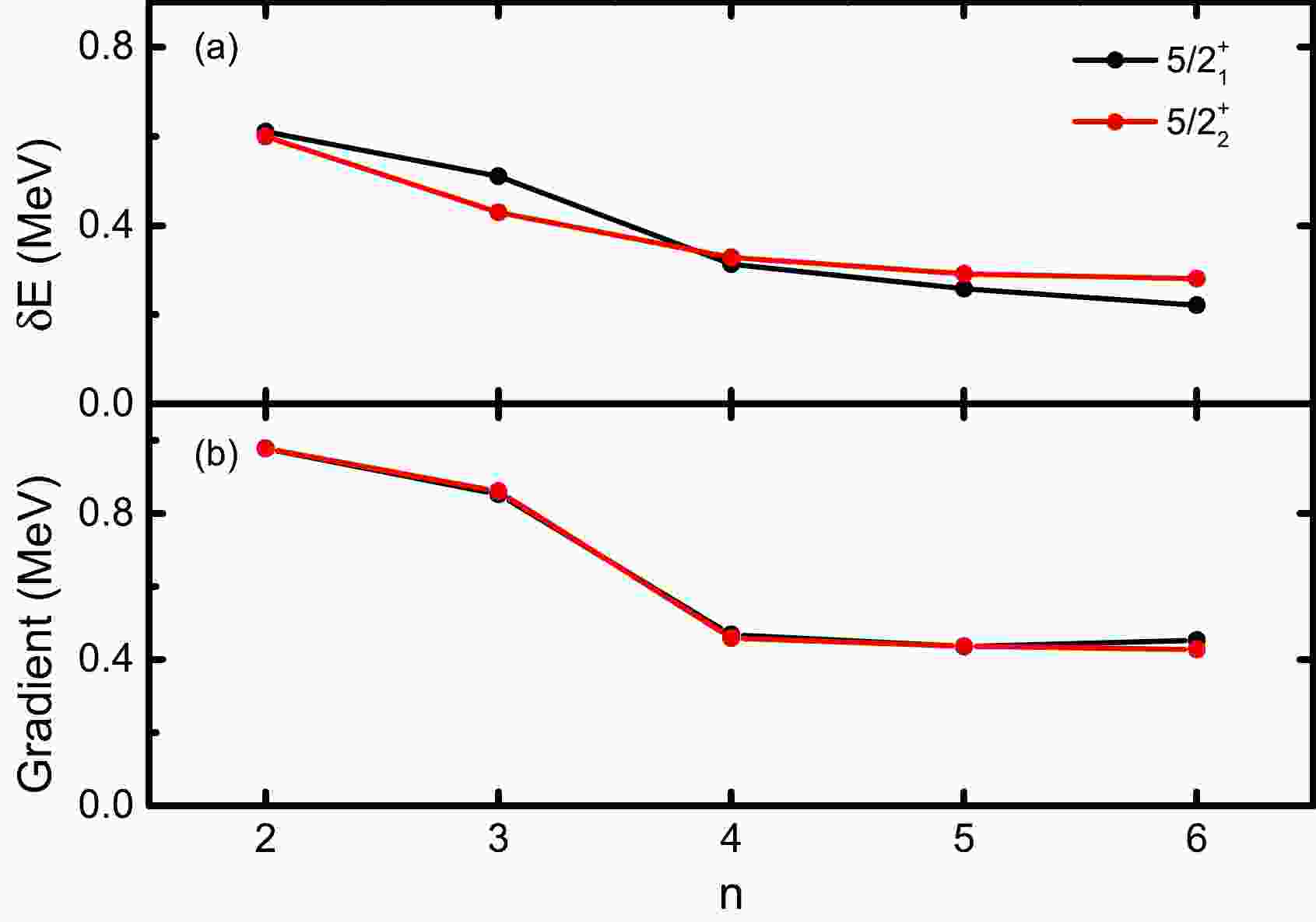
$ \nabla E^n_{J\alpha} $ member in$ \nabla S_m^n $ is also zero. To show this, we take$ ^{27} $ Al as a simple example and perform VAP calculations for the lowest two$ J^\pi=5/2^+ $ states in the$ sd $ shell with n ranging from$ 2 $ to$ 6 $ . Here, we take$ K=1/2 $ and adopt the USDB interaction [13]. The calculated energies and the absolute values of the corresponding energy gradients are shown in Fig. 1. The exact SM energies are calculated with the NUSHELLX code [14]. One can see that the differences between the converged VAP energies and the exact SM ones decrease with n. The two corresponding energy gradients are clearly far from zero but very close to each other because they are mutually canceled according to Eq. (7). However, such energy gradients also decrease gradually as n increases. This implies that smaller gradients may correspond to better approximation. At this point, one may expect that a converged VAP wave function with a fixed n can be further optimized if its energy gradient can be further reduced.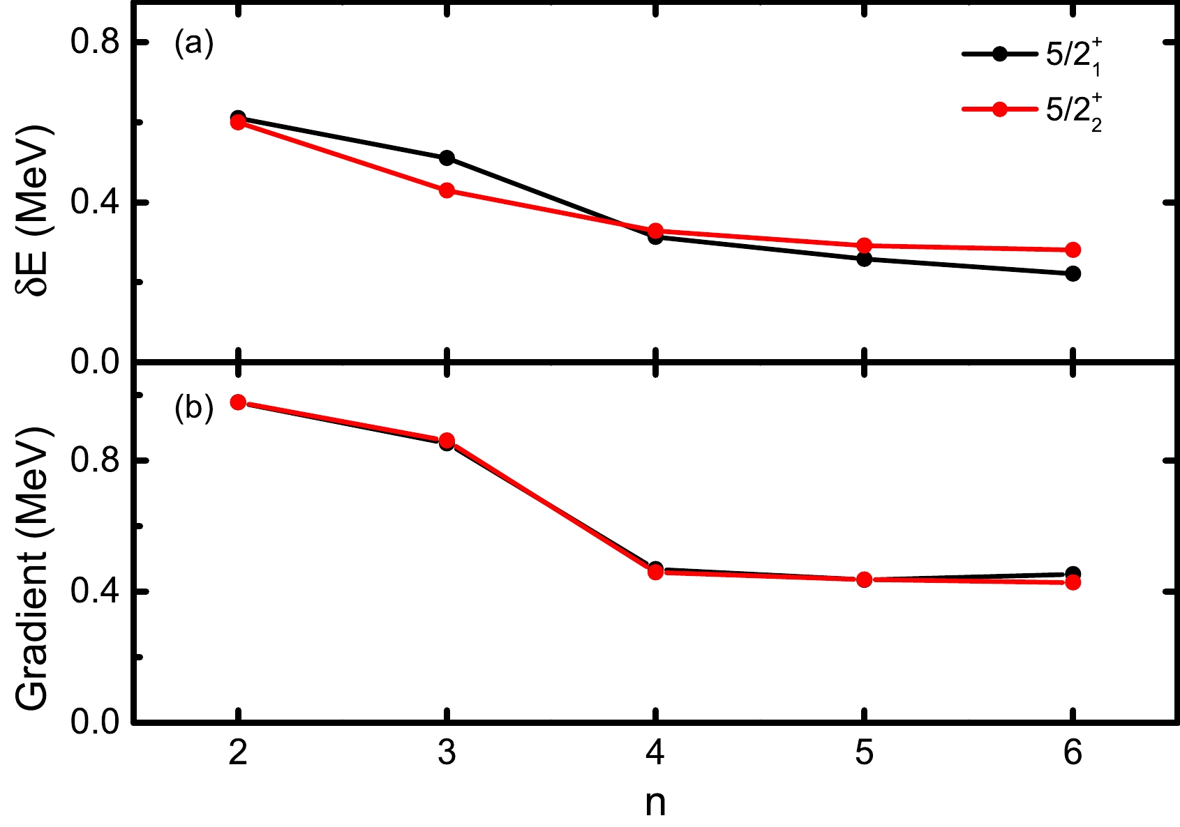
Figure 1. (color online) Calculated results for the lowest two
$ J^\pi=5/2^+ $ states in$ ^{27} $ Al with VAP. (a) Differences between the VAP energies and the exact SM ones with respect to the number of SDs n. (b) Absolute values of the corresponding gradients of the VAP energies when$ \nabla S_m^n=0 $ .The HUM theorem clearly states that, with a given Hamiltonian, the approximate energy, i.e.,
$ E^n_{J\alpha} $ , for any excited state must be at or above the corresponding SM eigenvalue,$ e_{J\alpha} $ . Thus if$ E^n_{J\alpha}=e_{J\alpha} $ , we must have$ \delta E^n_{J\alpha}[\Psi^{(n)}_{J\pi M\alpha}(K)]=\delta\frac{\langle\Psi^{(n)}_{J\pi M\alpha}(K)|\hat{H}|\Psi^{(n)}_{J\pi M\alpha}(K)\rangle}{\langle\Psi^{(n)}_{J\pi M\alpha}(K)|\Psi^{(n)}_{J\pi M\alpha}(K)\rangle}=0. $

(8) According to the Ritz variational principle [7], Eq. (8) is equivalent to the exact Schrödinger equation
$ \begin{array}{*{20}{l}} \hat{H}|\Psi^{(n)}_{J\pi M\alpha}(K)\rangle=e_{J\alpha}|\Psi^{(n)}_{J\pi M\alpha}(K)\rangle. \end{array} $

(9) Equation (9) indicates that when the approximate energy of the α-th state,
$ E^n_{J\alpha} $ , is equal to the corresponding SM eigenvalue, i.e.,$ e_{J\alpha} $ , the projected wave function must be also the same as the SM one regardless of what$ E^n_{Ji} (i<\alpha) $ is. Thus, the wave function for the α-th lowest state may be individually optimized by minimizing only the$ E^n_{J\alpha} $ energy. However, in practical calculations, the situation seems more complicated. In Fig. 2, we take the same VAP calculation used for Fig. 1 but only minimize the energy of the$ J^\pi=5/2_2^+ $ state with$ n=2 $ . The two initial projected states are generated randomly, and the calculated results are denoted by the black symbols. It is nice that both$ 5/2^+ $ energies decrease at early iterations, but later, the$ 5/2_1^+ $ energy gradually increases and becomes very close to the$ 5/2_2^+ $ energy. This stops the$ 5/2_2^+ $ state from being further optimized.
Figure 2. (color online) (a) Convergence pattern of the energies of the lowest two
$ J^\pi=5/2^+ $ states in$ ^{27} $ Al with$ (\omega_1, \omega_2)=(0,1) $ and$ (0.01,1) $ , respectively. (b) Absolute value of the corresponding gradient of the approximate energy of the$ J^\pi=5/2_2^+ $ state as a function of the iteration number. The USDB interaction is adopted.To ensure the convergence of such VAP iteration, we propose a weighted VAP method (called as WVAP), so that the
$ 5/2_1^+ $ energy may not be so close to the above$ 5/2_2^+ $ one. In this method, a real and positive weight factor,$ \omega_\alpha $ , is assigned to each$ E^n_{J\alpha} $ by hand. Then, the VAP calculation for the i-th lowest state is performed by minimizing the weighted energy sum:$ S_i^{n}=\sum\limits_{\alpha=1}^i \omega_\alpha E^n_{J\alpha}, $

(10) where
$ \omega_\alpha (\alpha<i) $ is expected to be far smaller than$ \omega_i $ . Of course, the WVAP can be reduced to the normal VAP when all the weight factors, i.e.,$ \omega_\alpha $ , in Eq. (10) are the same.To check the convergence of the present method, we repeat the above calculation to optimize the second lowest
$ J^\pi=5/2^+ $ state in$ ^{27} $ Al but with$ (\omega_1,\omega_2)=(0.01,1) $ adopted. The calculated results are denoted by the red symbols in Fig. 2. It is clearly shown that with a small weight of$ 0.01 $ assigned to the$ 5/2_1^+ $ energy, a gap between the two approximate energies appears, and the iteration now can be well converged. Correspondingly, the final absolute value of the gradient of the$ 5/2_2^+ $ energy is remarkably reduced, and it turns out to be approximately$ 0.05 $ MeV.In Fig. 3, one can see the improvement of WVAP compared with the original VAP results with different n numbers. The calculated energies from WVAP are generally more than 100 keV lower than those from VAP, and the former energies are closer to the exact shell model one. More interestingly, the WVAP energy with
$ n=3 $ is already as low as the VAP one with$ n=6 $ , which implies that the WVAP wave functions can be more compact. From Fig. 3(b), one can also see the difference between WVAP and VAP. The absolute values of the calculated gradients of the WVAP energies are far smaller than those of the corresponding VAP ones and are very close to zero. This indicates that the wave functions obtained from WVAP are indeed improved from VAP.
Figure 3. (color online) Calculated results for the
$ J^\pi=5/2_2^+ $ state in$ ^{27} $ Al with VAP and WVAP, respectively. (a) Differences between the approximate energies and the exact SM ones with respect to the number of SDs n. (b) Absolute values of the corresponding gradients of the approximate energies when the iteration converges. The USDB interaction is adopted.The next example is calculated in the
$ pf $ shell. We perform similar calculations for the$ J^\pi=0_2^+ $ ,$ 0_3^+ $ ,$ 2_2^+ $ , and$ 2_3^+ $ states in$ ^{48} $ Cr with$ K=0 $ . Here$ (\omega_1,\omega_2) $ is taken as$ (0.01,1) $ for both the$ 0_2^+ $ and$ 2_2^+ $ states, and$ (\omega_1,\omega_2,\omega_3) $ is taken as$ (0,0.01,1) $ for the$ 0_3^+ $ state. For the$ 2_3^+ $ state, the exact SM energy of the$ 2_2^+ $ state is close to that of the$ 2_3^+ $ state, whose energy difference is only approximately$ 0.7 $ MeV. In order to ensure the convergence for this$ 2_3^+ $ state, the weights of the lowest two$ 2^+ $ states are slightly increased to$ (\omega_1,\omega_2,\omega_3)=(0.01,0.1,1) $ . The GXPF1A interaction is adopted [15], and the calculated results are shown in Fig. 4. For all the calculated states, the energies obtained from WVAP are still lower than the corresponding VAP ones. Moreover, it seems that the improvement of the second excited states is better than that of the first excited states in WVAP.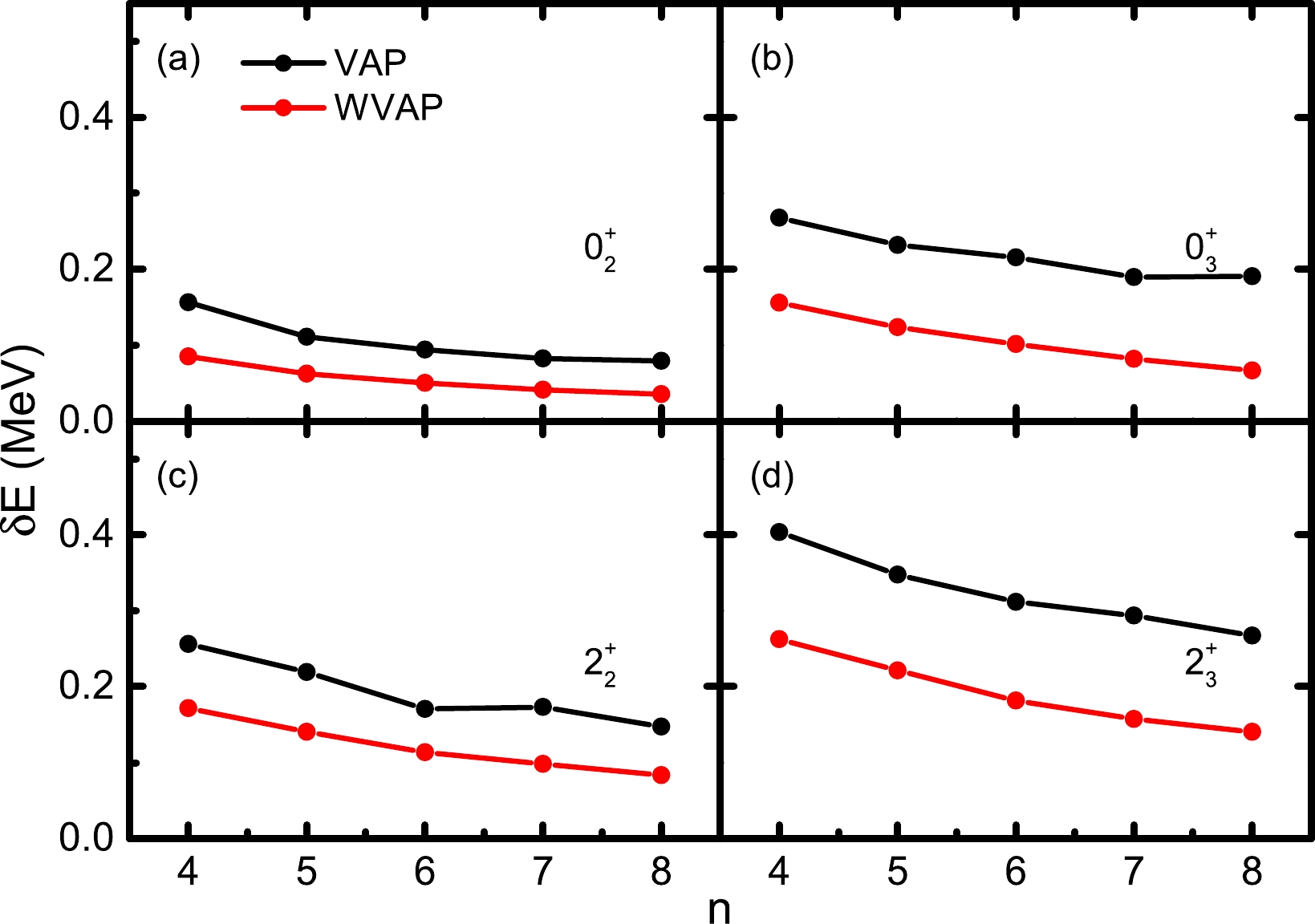
Figure 4. (color online) Energy differences between the approximate energies of nonyrast states in
$ ^{48} $ Cr obtained from VAP and WVAP and the exact SM ones with respect to the number of SDs n. (a)$ J^\pi=0_2^+ $ ; (b)$ J^\pi=0_3^+ $ ; (c)$ J^\pi=2_2^+ $ ; (d)$ J^\pi=2_3^+ $ .The
$ B(E2) $ values are also calculated using the wave functions corresponding to the energies with$ n=8 $ in Fig. 4. The calculated values are listed in Table 1. One can see that the$ B(E2) $ values obtained from both VAP and WVAP are in good agreement with the SM ones. Moreover, one can observe that the$ B(E2) $ values with WVAP are generally closer to the exact shell model ones, except for the$ 2_{2}^{\dagger}\rightarrow 0_{3}^{\dagger} $ transition.VAP WVAP SM $ 2_{2}^{\dagger}\rightarrow 0_{2}^{\dagger} $ 

$ 64.062 $ 

$ 59.491 $ 

$ 58.825 $ 

$ 2_{2}^{\dagger}\rightarrow 0_{3}^{\dagger} $ 

$ 0.492 $ 

$ 0.629 $ 

$ 0.453 $ 

$ 2_{3}^{\dagger}\rightarrow 0_{2}^{\dagger} $ 

$ 1.392 $ 

$ 1.240 $ 

$ 1.123 $ 

$ 2_{3}^{\dagger}\rightarrow 0_{3}^{\dagger} $ 

$ 19.257 $ 

$ 20.890 $ 

$ 22.941 $ 

Table 1.
$ B(E2,J\rightarrow J-2) $ (in${\rm e}^2$ fm$ ^4 $ ) values of the states in$ ^{48} $ Cr obtained using VAP, WVAP, and the SM.As an application of the present method to heavier nuclei, we calculate the lowest three
$ 0^+ $ states in$ ^{56} $ Ni with$ n=15 $ independently. Here,$ (\omega_1,\omega_2) $ is taken as$ (0.001,1) $ for the$ 0_2^+ $ state, and$ (\omega_1,\omega_2,\omega_3) $ is taken as$ (0.001,0.001,1) $ for the$ 0_3^+ $ state. The FPD6 interaction is adopted [16]. The calculated energies are$E(0_1^+)= -203.160$ MeV,$ E(0_2^+)=-198.611 $ MeV, and$E(0_3^+)= -198.147$ MeV, which are only$ 38 $ ,$ 112 $ , and$ 57 $ keV above the corresponding exact SM ones, respectively.A very similar study related to the minimization of Eq. (10) was performed by Puddu [17]. However, the present work is essentially different from that one. In the method of Ref. [17], when calculating an excited state with given quantum numbers, one must also calculate the wave functions for the yrast state and all the lower non-yrast states with the same quantum numbers. In contrast, in the present method, one can directly calculate an arbitrary highly excited state even without knowing the wave functions of any other states. This is a very useful feature of the present method for studying the high-lying excited states. The rationality of our method is still based on the HUM theorem, whose advantage seems not to be taken by Ref. [17]. From the HUM theorem, we know that all the approximate excited energies are always above the corresponding exact ones. The present algorithm is designed so that the calculated excited energy can be as low as possible. Therefore, the best approximation for this state can be achieved with a given number of projected basis states.
Because the wave functions for the excited states are optimized independently, they are not obtained from the same diagonalization. This may lead to non-orthogonality among the calculated wave functions. In principle, this problem can be easily solved by performing a final diagonalization in the space spanned by all the projected basis states taken from all the calculated wave functions. However, it is known that the exact wave functions are strictly orthogonal; thus, if the calculated WVAP wave functions have sufficiently good approximations, their orthogonality should be automatically fulfilled, and such final diagonalization may be less important. For instance, in the calculations of Fig. 4, all the overlaps among the calculated WVAP wave functions of different states with
$ n=8 $ are within 0.003.There is another difference between the present work and Ref. [17]. In Puddu's work, the projected SDs are varied one by one. In contrast, here, all the included projected SDs are varied simultaneously. Although the computational costs are higher, one may expect that the present WVAP wave functions are more compact. The above WVAP energies of the lowest three
$ 0^+ $ states in$ ^{56} $ Ni with$ n=15 $ , indeed, are slightly lower than the results obtained with the same number of SDs in Ref. [17]. -
Theoretically, in any approximate SM method, the obtained energies can be close to the exact SM ones to any extent as long as the adopted configuration subspace is large enough. Without exception, in VAP or WVAP, a large number of SDs are also required if one wants to obtain the precise eigenenergies of a Hamiltonian. However, this is impossible because VAP calculations with large n are very computationally expensive. Alternatively, the exact SM energies may be estimated according to the approximate VAP or WVAP wave functions. Such energy estimation can be done by adopting the energy-variance extrapolation method, which has been introduced in the nuclear physics [18].
Given a Hamiltonian
$ \hat{H} $ , the energy variance with respect to an approximate SM wave function, i.e.,$ |\Psi^{(n)}_{J\pi M\alpha}(K)\rangle $ , is defined as$ \begin{aligned}[b] \Delta E^n_{J\alpha}=&\langle\Psi^{(n)}_{J\pi M\alpha}(K)|(\hat{H}-E^n_{J\alpha})^2|\Psi^{(n)}_{J\pi M\alpha}(K)\rangle\\ =&\langle\Psi^{(n)}_{J\pi M\alpha}(K)|\hat{H}^2|\Psi^{(n)}_{J\pi M\alpha}(K)\rangle-{E^n_{J\alpha}}^2. \end{aligned} $

(11) Details regarding how to compute the matrix elements of the energy variance can be found in Ref. [9]. As shown in Ref. [18], if
$ \Delta E^n_{J\alpha} $ is not too large,$ E^n_{J\alpha} $ can be approximately expressed as a quadratic function of its energy variance, i.e.,$ \begin{array}{*{20}{l}} E^n_{J\alpha}\approx a{\Delta E^n_{J\alpha}}^2+b\Delta E^n_{J\alpha}+c, \end{array} $

(12) where a, b, and c are parameters to be fitted with a series of
$ (\Delta E^n_{J\alpha}, E^n_{J\alpha}) $ values. Considering the fact that$ |\Psi^{(n)}_{J\pi M\alpha}(K)\rangle $ must be an exact SM wave function if$ \Delta E^n_{J\alpha}=0 $ , the parameter c can be regarded as an estimation of the exact SM energy.In previous works [9, 19–21], the energy-variance extrapolation has been performed with various approximate SM wave functions, including those from VAP. All those extrapolations work well in the prediction of exact SM energies of the low-lying states provided the approximations of the adopted wave functions are good enough. However, for nonyrast states, the WVAP is able to further optimize the normal VAP wave functions. This is definitely helpful for increasing the precision of the energy-variance extrapolation for the calculated nonyrast states.
To confirm this point, we perform the WVAP calculations for the
$ 5/2_2^+ $ state in$ ^{27} $ Al starting from$ n=2 $ . We still take$ K=1/2 $ and$ (\omega_1,\omega_2)=(0.01,1) $ . Once the WVAP iteration with n converges, a new projected SD is added to this converged wave function, and the next WVAP iteration with$ n+1 $ is performed. One can keep increasing n so that the converged WVAP energy can be continuously reduced. Here, we stop adding projected SDs when$ n=12 $ . For comparison, Fig. 5 shows the$ (\Delta E^n_{J\alpha}, E^n_{J\alpha}) $ values calculated from WVAP and VAP with n ranging from 2 to 12. One can see that the$ (\Delta E^n_{J\alpha}, E^n_{J\alpha}) $ values from WVAP are significantly smaller than those from VAP with the same n. Moreover, such quantities from WVAP with$ n=7 $ are even smaller than those from VAP with$ n=12 $ . This good improvement of the WVAP results convinces us that the quality of the energy extrapolation may be significantly improved. To estimate the exact SM energy, the last$ 6 $ points of the$ (\Delta E^n_{J\alpha}, E^n_{J\alpha}) $ values are used for the curve fitting with Eq. (12). The extrapolated energies are the c numbers, which are the intercepts of the fitted lines at the vertical (energy) axis with the energy variance being zero. From Fig. 5, it is clearly observed that the extrapolated energy with WVAP is very close to the exact SM ones within a$ 10 $ -keV difference, while the result with VAP seems unsuccessful owing to a lack of sufficiently good approximation of the VAP wave functions. Certainly, precise energy extrapolation also can be achieved with VAP if more projected SDs are included in the VAP wave functions, but this will take too much computational time.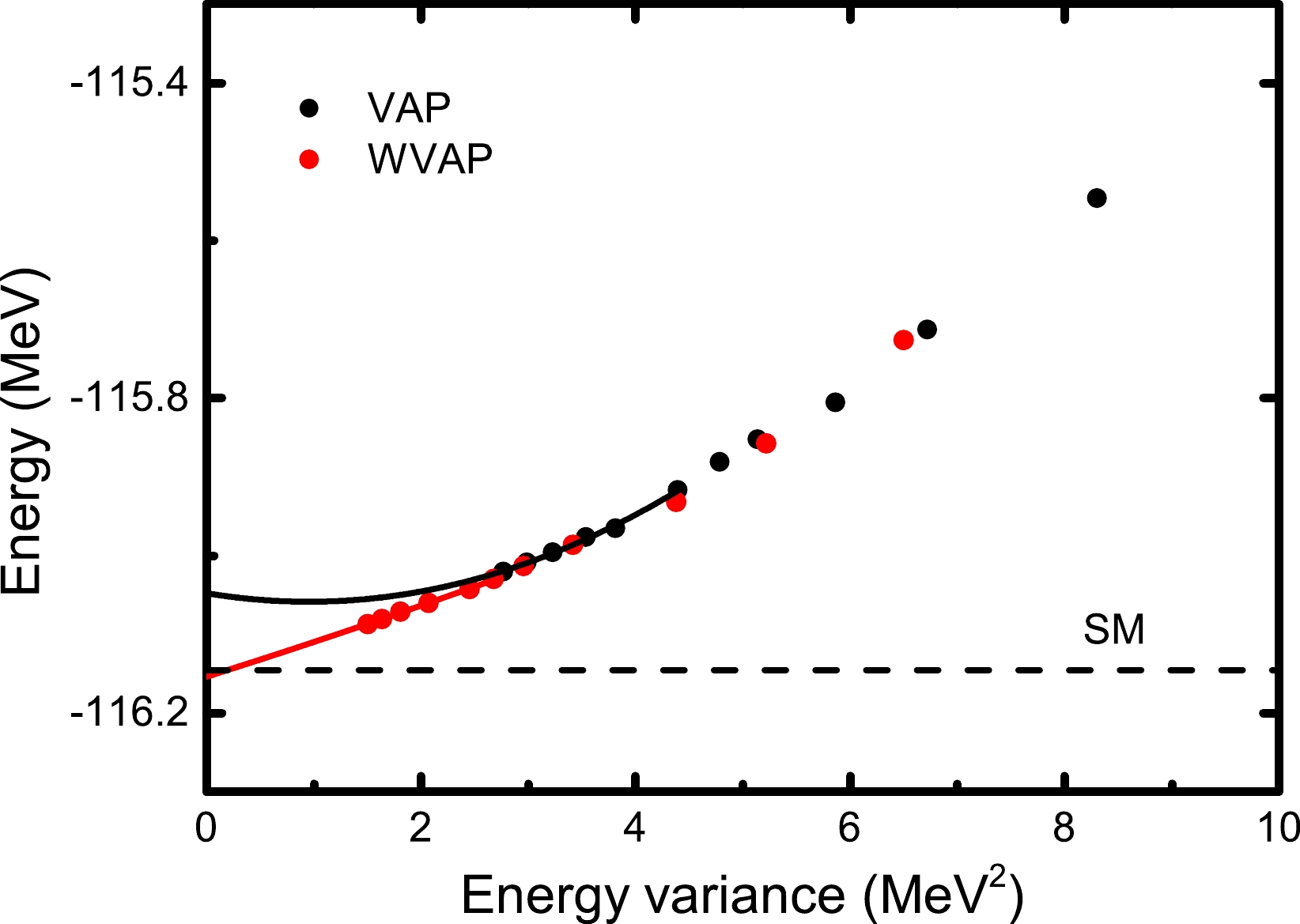
Figure 5. (color online) Energy extrapolations with Eq. (12) for the
$ J^\pi=5/2_2^+ $ state in$ {^{27}} $ Al based on the wave functions from VAP and WVAP. The solid black (red) symbols and solid black (red) lines denote the VAP (WVAP) results and their second-order fit, respectively. The exact SM energy is indicated by the dashed line. The USDB interaction is adopted.As a more practical application, we further perform energy extrapolations for the energies of the
$ 0_2^+ $ ,$ 0_3^+ $ ,$ 2_2^+ $ , and$ 2_3^+ $ states in$ ^{48} $ Cr in the$ pf $ model space. In this case, we still take$ K=0 $ and adopt the GXPF1A interaction. The same weights used in the above section are adopted. For each state, the extrapolated results are also obtained by fitting the last$ 6 $ points. The calculated results are shown in Fig. 6. For all the calculated states, the extrapolated energies are in excellent agreement with the exact SM ones, and all the deviations of the estimated values are within$ 10 $ keV.
Figure 6. (color online) Energy extrapolations with Eq. (12) for the
$ J^\pi=0_2^+ $ ,$ 0_3^+ $ ,$ 2_2^+ $ , and$ 2_3^+ $ states in$ {^{48}} $ Cr based on the WVAP wave functions. The solid symbols and solid lines denote the WVAP results and their second-order fits, respectively. The open symbols denote the corresponding VAP values with the same n. The exact SM energies are indicated by the dashed lines. The GXPF1A interaction is adopted. -
We have proposed a weighted VAP method to further improve the original VAP wave functions for low-lying nonyrast states. In the previous VAP, the low-lying states are calculated by minimizing the sum of the lowest energies. In this study, a weight factor is attached to each calculated energy, and then, the sum of these weighted energies is minimized. When calculating a nonyrast state that we are interested in, the weight for the corresponding energy is set to be far larger than the other factors. Our calculations clearly show that the WVAP can significantly improve the approximation of the original VAP. However, owing to the limited number of included projected SDs, the obtained WVAP energies are approximate ones. Nevertheless, one can estimate the exact shell model energies according to the WVAP results by adopting the energy-variance extrapolation method. Our calculations indicate that such wave functions improved by the WVAP method indeed present excellent energy extrapolations with deviations less than 10 keV.
As a proof-of-the-principle study, the calculations in the present work mainly focus on the low-lying nonyrast states of nuclei within the capacity of the shell model. One may be interested in how well it works when it is applied to heavy nuclei. Additionally, the weight of each state is assigned by hand, which is somewhat inconvenient. It is necessary to develop a novel algorithm to determine the weights in a consistent way. Such work is in progress.
Weighted variation after projection method for low-lying nonyrast states
- Received Date: 2023-02-24
- Available Online: 2023-07-15
Abstract: We propose a simple algorithm to further improve the previous variation after projection (VAP) wave functions for low-lying nonyrast states. We attach a weight factor to each calculated energy; then, the sum of these weighted energies is minimized. It turns out that a low-lying nonyrast VAP wave function can be further optimized when the weight factor for the corresponding energy is far larger than the other ones. Based on the improved WVAP wave functions, the energy-variance extrapolation method is applied to estimate the exact shell model energies. The calculated results for nuclei in the


 DownLoad: