


 Abstract
 HTML
HTML Reference
 Related
 PDF
PDF


-
Owing to the progress made by gravitational wave detectors [1] and the Event Horizon Telescope [2, 3], we have a profound understanding of black holes. Nowadays, general relativity remains the most widely accepted theory of gravity. However, singularities are unavoidable in terms of the law of singularity [4, 5], which can be proved if the spacetime described by general relativity has a certain overall structure and meets the strong energy condition. The existence of singularities not only destroys the completeness of spacetime but also makes all physical laws, including general relativity itself, fail at the singularities. Therefore, it is highly expected to eliminate the singularities. A black hole that has no singularities in spacetime, i.e., its center is not a singularity, is called a "regular black hole" [6]. The first regular black hole was constructed by Bardeen [7] and was later interpreted [8] as the solution of the gravitational field coupled with the magnetic monopole field of nonlinear electrodynamics. Subsequently, more regular black holes were constructed under a variety of physical motives. Among them, representative regular black holes are the Hayward black hole [9], the noncommutative spacetime inspired black hole [10], and the regular black hole from the loop quantum gravity [11], etc. We note that these regular black holes are static and spherically symmetric, whereas the regular black holes that would exist in nature are most probably rotating and axially symmetric. For a static and spherically symmetric black hole with singularities, the Newman-Janis algorithm (NJA) can be used [12] to transform it into a rotating and axially symmetric black hole. However, for a static and spherically symmetric regular black hole without singularities, the NJA does not give a unique rotating and axially symmetric regular black hole, because the complex parameterization of radial coordinates has flexibility to a certain extent [13−15]. To this end, the modified NJA was proposed [16, 17] for a static and spherically symmetric black hole, which constrains the complex parameterization of radial coordinates through the global nature of coordinate transformations and thus leads to a unique rotating black hole solution. In this study, we analyze rotating regular black holes in terms of the modified NJA.
As is already known, singular black holes (black holes with singularities) have spacetime structures different from those of regular black holes [18−21]. Because the event horizon of a black hole shields the region inside a black hole [22], the internal structure of a black hole cannot be detected directly. Therefore, the description of internal structures needs to rely on the interaction between a black hole and its external matter or the gravitational field. Here, we focus on an interesting phenomenon, i.e., the "superradiance" [23−27], which refers to the phenomenon that the energy of a particle can be amplified and reflected back by the black hole when the particle incident on a black hole meets certain conditions. Based on the superradiance, if a particle is reflected by a "mirror" outside a black hole, the particle's energy will increase exponentially near the event horizon of the black hole, which is also known as a "black hole bomb" or "superradiance instability" [28−30]. When a massive scalar particle is in its bound state, the mass term can act as a mirror [31−35], making superradiance instability possible. The superradiance related effects, i.e., the superradiance instability and the energy extraction efficiency, are mainly affected by the properties of black hole spacetime; thus, the behavior of scalar particles satisfying the conditions of superradiance will reveal the properties of black hole spacetime. In the past, superradiance was studied [36−41] mainly for singular black holes but rarely for rotating regular black holes. Considering the fact that the superradiance associated with rotating regular black holes plays an indispensable role in black hole physics, we address this gap. Moreover, we shall better understand the properties of regular black holes when we study the superradiance phenomena affected by regularization parameters. This is because the spacetime singularities can be removed by introducing regularization parameters into the metrics of singular black holes. Therefore, starting from the bound state of a massive scalar particle, we deal with analytically the superradiance instability under the background of a rotating regular black hole constructed by the modified NJA, and then from the free state of the scalar particle, we calculate the energy amplification factor. For two specific models, i.e., the rotating Hayward and Bardeen black holes, we perform numerical calculations and image analyses in order to show the influence of regularization parameters on the superradiance effects of the two models. By comparing the results of the two specific models with that of the Kerr black hole, we can show the differences in superradiance between rotating regular black holes and rotating singular black holes.
The remainder of this paper is organized as follows. In Sec. II, we briefly introduce rotating regular black holes and massive scalar field equations. In Sec. III, we determine the conditions of superradiance instability by using the asymptotic matching method when a massive scalar particle is at its bound state. For the scattering process of a free state particle, we calculate the superradiance amplification factor in Sec. IV. For the two specific models, we discuss in Sec. V how the superradiance behaviors of the rotating Hayward and Bardeen black holes vary with respect to their respective regularization parameters and rotation parameters and compare them with the superradiance behavior of Kerr black holes (a type of rotating singular black hole). Finally, we provide our conclusions in Sec. VI, including some comments and further extensions. Throughout the paper, we adopt the natural units
$ \hbar=c=G=1 $ . -
It is considerably difficult to obtain the solutions of rotating black holes from the Einstein field equations, because the complexity of Einstein's field equations in the rotating case is far higher than that in the static case. Therefore, the widely used method for constructing rotating black holes is the NJA [12]. This algorithm originated from the connection between a static black hole and a rotating one in general relativity. It is well known that the Schwarzschild, Reissner-Nordström (RN), Kerr, and Kerr-Newman (KN) black holes were obtained by solving Einstein's field equations in vacuum. By comparing the metrics of these black holes, Newman and Janis proposed the transformation from the static and spherically symmetric Schwarzschild black hole to the rotating and axially symmetric Kerr black hole. Moreover, the algorithm can realize the transformation from the RN black hole to the KN black hole.
However, for most static regular black holes with spherical symmetry, the corresponding rotating regular black holes with axial symmetry cannot be uniquely determined, owing to the uncertainty of the complex parametrization of radial coordinates. According to the constraint of the global coordinate transformation, the modified NJA without complexification was proposed [16, 17]. Here, we briefly introduce the rotating regular black holes constructed by this algorithm.
As far as we know, the regular black holes with spherical symmetry in general relativity are described by the following line element:
$ {\rm d}s^2=-F(r){\rm d}t^2+\frac{{\rm d}r^2}{F(r)}+r^2({\rm d}\theta^2+\sin^2\theta {\rm d}\phi^2), $

(1) where
$ F(r) $ contains the black hole mass M. In the advanced null coordinates$ (u,r,\theta,\phi) $ defined by$ \mathrm{d} u= \mathrm{d} t-\frac{ \mathrm{d} r}{F(r)}, $

(2) one expresses the contravariant form of the metric in terms of a null tetrad:
$ g^{\mu\nu}=-l^\mu n^\nu-l^\nu n^\mu+m^\mu m^{*\nu}+m^\nu m^{*\mu}, $

(3) where
$ l^\mu=\delta^\mu_r, \tag{4a} $

$ n^\mu=\delta^\mu_u-\frac{F}{2}\delta^\mu_r, \tag{4b}$

$ m^\mu=\frac{1}{\sqrt{2r^2}}\left(\delta^\mu_\theta+\frac{\rm i}{\sin\theta}\delta^\mu_\phi\right),\tag{4c} $

$ l_\mu l^\mu=m_\mu m^\mu=n^\nu n_\nu=l_\mu m^\mu=n_\mu m^\mu=0, \tag{4d} $

$ l_\mu n^\mu=-m_\mu m^{*\mu}=1, \tag{4e} $

and "
$ * $ " denotes the complex conjugate. Then, one introduces the rotation via the complex transformation$ r\rightarrow r+{\rm i} a\cos\theta,\qquad u\rightarrow u-{\rm i} a\cos\theta, $

(5) where a is a rotation parameter, and requires that
$ \delta^\mu_\nu $ transform as a vector under the complex transformation$\begin{aligned}[b] & \delta^\mu_r\rightarrow \delta^\mu_r, \qquad \delta^\mu_u\rightarrow \delta^\mu_u, \\& \delta^\mu_\theta\rightarrow \delta^\mu_\theta+ {\rm i} a\sin\theta(\delta^\mu_u-\delta^\mu_r), \qquad \delta^\mu_\phi\rightarrow \delta^\mu_\phi. \end{aligned} $

(6) For a singular black hole, the metric function of its rotating counterpart can be determined under this complex transformation rule. However, such a transformation rule does not work well for a regular black hole. Thus, one assumes that
$ \{F,r^2\} $ transforms into$ \{B,\Psi\} $ :$ \{F(r),r^2\}\rightarrow \{B(r,\theta,a),\Psi(r,\theta,a)\}, $

(7) where
$ \{B,\Psi\} $ are real functions to be determined and should recover their static counterparts in the limit of$ a\rightarrow 0 $ , i.e.,$ \lim\limits_{a\to 0}B(r,\theta,a)=F(r),\qquad \lim\limits_{a\to 0}\Psi(r,\theta,a)=r^2. $

(8) According to Eqs. (6) and (7), the null tetrad becomes
$ l^\mu=\delta^\mu_r, \tag{9a} $

$ n^\mu=\delta^\mu_u-\frac{B}{2}\delta^\mu_r, \tag{9b} $

$ m^\mu=\frac{1}{\sqrt{2\Psi}}\left[\delta^\mu_\theta+{\rm i}a\sin\theta(\delta^\mu_u-\delta^\mu_r)+\frac{\rm i}{\sin\theta}\delta^\mu_\phi\right], \tag{9c} $

and the corresponding line element with rotation takes the form
$ \begin{aligned}[b] \mathrm{d} s^2=& -B \mathrm{d} u^2-2 \mathrm{d} u \mathrm{d} r-2a\sin^2\theta\left(1-B\right) \mathrm{d} u \mathrm{d} \phi+2a\sin^2\theta \mathrm{d} r \mathrm{d} \phi\\ & +\Psi \mathrm{d}\theta^2+\sin^2\theta\left[\Psi+a^2\sin^2\theta\left(2-B\right)\right] \mathrm{d}\phi^2. \end{aligned} $

(10) Next, one rewrites the above line element with the Boyer-Lindquist coordinates and lets the metric have only one non-vanishing off-diagonal term
$ g_{t\varphi} $ . To reach the aim, one needs the following coordinate transformation:$ \mathrm{d} u= \mathrm{d} t+\lambda(r) \mathrm{d} r,\qquad \mathrm{d}\phi= \mathrm{d}\varphi+\chi(r) \mathrm{d} r, $

(11) where
$ \{\lambda(r),\chi(r)\} $ depend only on r in order to ensure integrability. If the transformation Eq. (7) is determined a priori,$ \{\lambda(r),\chi(r)\} $ may not exist. Considering these constraints, one has the formulations of$\{B(r,\theta,a), \Psi(r,\theta), \lambda(r), \chi(r)\}$ :$ B(r,\theta)=\frac{Fr^2+a^2\cos^2\theta}{\Psi}, \tag{12a} $

$ \Psi(r,\theta)=r^2+a^2\cos^2\theta, \tag{12b} $

$ \lambda(r)=-\frac{r^2+a^2}{Fr^2+a^2},\tag{12c} $

$ \chi(r)=-\frac{a}{Fr^2+a^2}. \tag{12d}$

As a result, one obtains the line element for rotating regular black holes with the Kerr-like form:
$ \begin{aligned}[b] {\rm d}s^2=&-\left(1-\frac{2f}{\rho^2}\right){\rm d}t^2+\frac{\rho^2}{\Delta}{\rm d}r^2-\frac{4af\sin^2\theta}{\rho^2}{\rm d}t{\rm d}\varphi\\&+\rho^2{\rm d}\theta^2+\frac{\Sigma \sin^2\theta}{\rho^2}{\rm d}\varphi^2, \end{aligned} $

(13) where
$ \rho^2=r^2+a^2\cos^2\theta, $

(14) $ 2f=r^2(1-F), $

(15) $ \Delta=r^2F+a^2=r^2-2f+a^2, $

(16) $ \Sigma=(r^2+a^2)^2-\Delta\, a^2\sin^2\theta=(r^2+a^2)\rho^2+2fa^2\sin^2\theta. $

(17) The regularity of the above rotating regular black holes can be verified because the Ricci scalar R and Kretschmann scalar K are finite everywhere. The reason is that the static regular black hole as a seed has de Sitter-like behavior in the limit of
$ r\rightarrow 0 $ [16, 17]:$ F(r)\sim 1-Cr^2\qquad {\rm{with}}\qquad C>0. $

(18) On the other hand, one can determine the horizon
$ r_{\rm H} $ by solving the algebraic equation$ g_{tt}g_{\varphi\varphi}-g_{t\varphi}^2=-\Delta\sin^2\theta=0 $ , which can be reduced to$ \theta=0 $ or$ r^2-2f+a^2=0. $

(19) In the remainder of this section, we turn to massive scalar field equations. In a curved spacetime, a massive scalar field
$ \Phi(t, r, \theta, \varphi) $ with the mass μ is described by$ \nabla^\nu\nabla_\nu\Phi=\mu^2\Phi. $

(20) In order to separate variables in the rotating regular black hole spacetime described by Eq. (13), we make the assumption
$ \Phi(t, r, \theta, \varphi)={\rm e}^{-{\rm i}\omega t+{\rm i}m\varphi}S(\theta)R(r), $

(21) and then we obtain the equations that govern
$ S(\theta) $ and$ R(r) $ :$ \begin{aligned}[b] & \frac{1}{\sin\theta}\frac{{\rm d}}{{\rm d}\theta}\left[\sin\theta\frac{{\rm d}}{{\rm d}\theta}S(\theta)\right] \\ +& \left[a^2(\omega^2-\mu^2)\cos^2\theta-\frac{m^2}{\sin^2\theta}+\lambda\right]S(\theta)=0, \end{aligned}$

(22) and
$ \begin{aligned}[b] &\Delta\frac{{\rm d}}{{\rm d}r}\left[\Delta \frac{{\rm d}}{{\rm d}r}R(r)\right]+\Big[\omega^2(r^2+a^2)^2-4afm\omega\\ +& a^2m^2-\Delta(\mu^2r^2+\lambda+a^2\omega^2)\Big]R(r)=0, \end{aligned}$

(23) respectively, where ω represents the frequency of the massive scalar field, m represents the azimuthal number with respect to the rotation axis, and λ is the separation parameter, which will be fixed approximately as an eigenvalue of Eq. (22).
-
We discuss the eigenvalue of Eq. (23) under the boundary conditions of outgoing waves at infinity and ingoing waves at an event horizon. If the mass μ is small (see the following details), we shall show that the eigenvalue of Eq. (23) is exactly
$ \omega^2 $ , where ω is also called the eigenfrequency and is complex:$ \omega=\omega_{\rm R}+{\rm i}\omega_{\rm I}. $

(24) If
$ \omega_{\rm I}>0 $ ,$ \phi(t, r, \theta, \varphi) $ increases exponentially with time, as given by Eq. (21), which leads to instability, i.e., the superradiance instability. In order to analyze the condition that the superradiance instability occurs, we deal with$ \omega_{\rm I} $ as a positive quantity in the following discussions. In general, we have the condition$ \omega_{\rm R}\gg \omega_{\rm I} $ , which means that a black hole is perturbed by a scalar field, leading to a slow change of$ \phi(t, r, \theta, \varphi) $ with respect to time, that is,$ \omega_{\rm I} $ is small when compared with$ \omega_{\rm R} $ .In order to solve Eq. (23) analytically in terms of the asymptotic matching method [33], which is illustrated in Fig. 1, we have to make the approximations
$ \mu M\ll 1 $ and$ |\omega| M\ll 1 $ , i.e., μ is small and on the same order of magnitude as$ |\omega| $ . Using these approximations and considering that the order of magnitude of a is less than or equal to that of M, which means that$ \mu a\ll1 $ and$ |\omega|a\ll 1 $ , we find that the solution of Eq. (22), i.e.,$ S(\theta) $ , is just the spherical harmonics. Simultaneously, we fix the separation parameter$ \lambda\approx l(l+1) $ , where$ l=1, 2,... $ is called the multipole number. Next, we focus on Eq. (23). The key idea of the asymptotic matching method is to solve Eq. (23) approximately in the near horizon region and in the far region and then match the coefficients of the two solutions in the overlapping region of the two regions, to determine the general solution.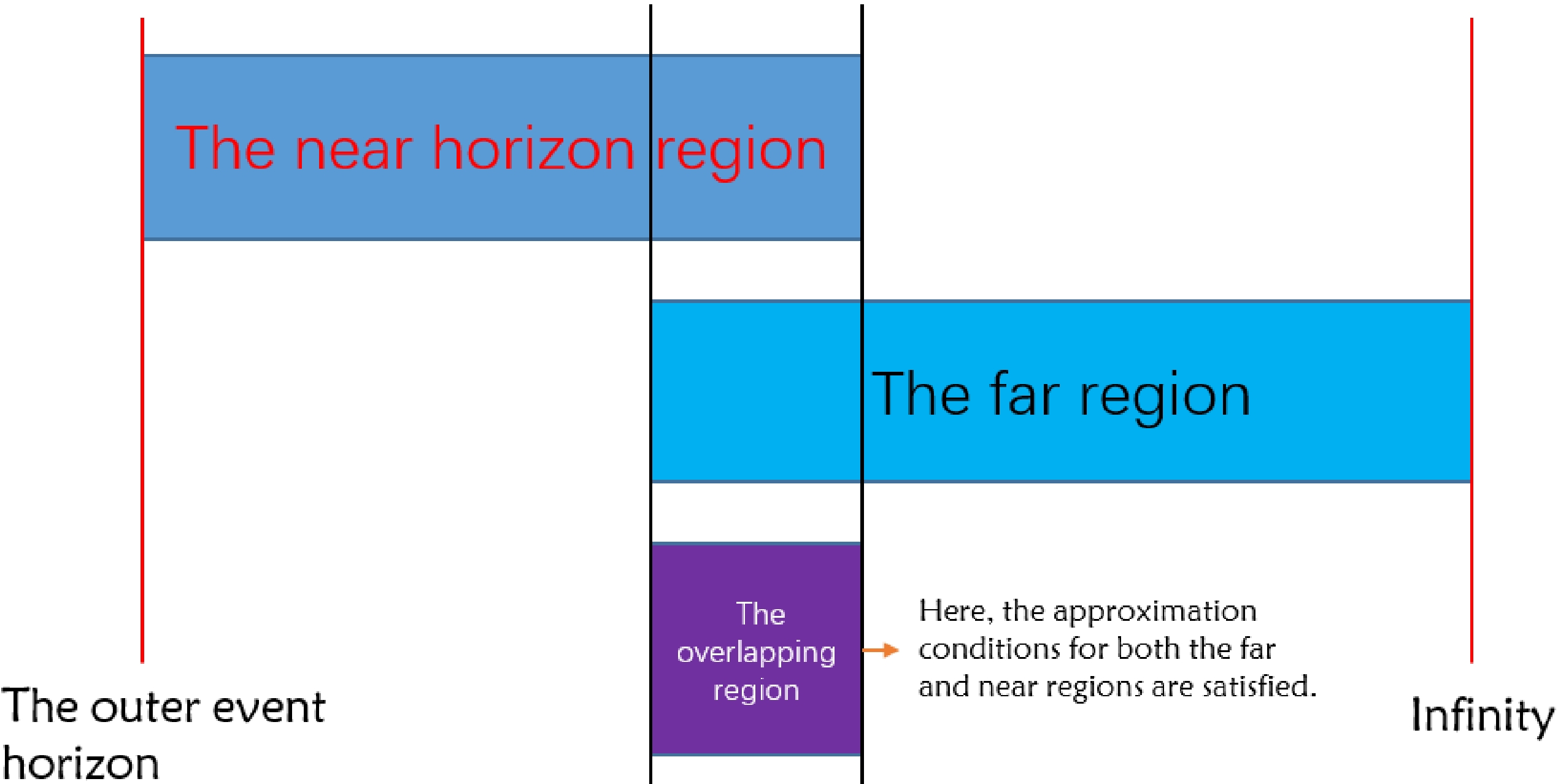
Figure 1. (color online) Schematic of the asymptotic matching method. In the near horizon region and the far region, the wave function behaves as two different solutions. The asymptotic behavior of the two solutions should be consistent in the overlapping region. Through this consistency, we can determine the coefficients of the wave function.
In the first step of the asymptotic matching method, we search for the asymptotic form of the far region solution in the near horizon region, which includes two sub-steps: the first is to compute the far region solution and the second is to give its asymptotic form in the near horizon region. In the far region,
$ r\gg M $ ; also, for the quantities with an order of magntiude less than or equal to that of M, such as a, i.e.,$ r\gg a $ , Eq. (23) can be approximately simplified as$ r^2\frac{{\rm d}}{{\rm d}r}\left[r^2\frac{{\rm d}}{{\rm d}r}R(r)\right]+\left[\omega^2r^4-\mu^2r^4+2\mu^2r^2f(r)-\lambda r^2\right]R(r)=0, $

(25) where
$ \omega^2 $ acts as the eigenvalue. In the above equation, the only uncertain factor is$ f(r) $ , which satisfies$ 2f(r)=r^2[1-F(r)] $ ; see Eq. (15). Notice that$ F(r)\sim 1 $ in the far region because the spacetime is asymptotically flat. We expand$ F(r) $ as the series of$ 1/r $ :$ F(r)=1+A\cdot\frac{1}{r}+B\cdot\frac{1}{r^2}+O\left(\frac{1}{r^3}\right), $

(26) where
$ A=\left.-r^2\dfrac{{\rm d}F(r)}{{\rm d}r}\right|_{r\rightarrow \infty} $ and$ B=\left.\dfrac{r^2}{2}\dfrac{{\rm d}}{{\rm d}r}\left[r^2\dfrac{{\rm d}F(r)}{{\rm d}r}\right]\right|_{r\rightarrow \infty} $ . Here, we consider the situation where both A and B converge. Note that A has the same order of magnitude as M, and B has the same order of mantiduge as$ M^2 $ , because the far region can also be written as$ M/r\ll 1 $ . After Eqs. (15) and (26) are considered together with$ \lambda\approx l(l+1) $ , Eq. (25) can be further simplified as$ \frac{{\rm d^2}}{{\rm d}r^2}\left[rR(r)\right]+\left[\omega^2-\mu^2-\frac{A\mu^2}{r}-\frac{l(l+1)}{r^2}\right]rR(r)=0. $

(27) When we use the definitions and notations
$ k^2\equiv \mu^2-\omega^2, $

(28) $ \nu\equiv -\frac{A\mu^2}{2k}, $

(29) $ x\equiv 2kr, $

(30) Eq. (27) becomes
$ \frac{{\rm d^2}}{{\rm d}x^2}\left[xR(x)\right]+\left[-\frac{1}{4}+\frac{\nu}{x}-\frac{l(l+1)}{x^2}\right]xR(x)=0. $

(31) Its solution with the boundary condition of an outgoing wave in the far region takes the form
$ R(x)= C_1 x^l {\rm e}^{-x/2}U(l+1-\nu,2l+2,x), $

(32) where
$ U(a,b,x) $ is the second Kummer function [42] and$ C_1 $ is an integration constant. Thus, we finish the first sub-step mentioned above. We make some comments regarding Eq. (32). It turns exactly into the solution of hydrogen atoms when ν is an integer. When we solve Eq. (31) for bound states, the most significant difference between a hydrogen atom and the present case lies in the asymptotic behavior for a small$ |x| $ . For a hydrogen atom, where x and ν are real, the wave function is required to be finite at$ x=0 $ , while for the present case, the scalar field interacts with the rotating regular black hole, leading to a slow change of the wave function, i.e., to the appearance of a small$ \omega_{\rm I} $ . Thus, ν, like ω, is complex because of the relationship between ω and ν; see Eqs. (28) and (29). If we define$ \delta\nu $ as$ n+\delta \nu\equiv \nu-l-1, $

(33) where n is a non-negative integer,
$ \delta\nu $ is a complex number with a small modulus. We can rewrite Eq. (32) as$ R(x)= C_1 x^l {\rm e}^{-x/2}U(-n-\delta \nu,2l+2,x). $

(34) Now, we turn to the second sub-step mentioned above, that is, to give the asymptotic form of the far region solution (Eq. (34)) in the near horizon region. Considering the condition
1 $ |x|\ll 1 $ or$ |k|r\ll 1 $ and expanding the second Kummer function in Eq. (34), we obtain the asymptotic behavior in the near horizon region:$ \begin{aligned}[b] R(x)\approx & C_1\left[ (-1)^n\frac{(2l+1+n)!}{(2l+1)!}x^l+(-1)^{n+1}(2l)!n!(\delta\nu) x^{-l-1}\right] \\ = & C_1(-1)^n\frac{(2l+1+n)!}{(2l+1)!}(2k)^l\cdot r^l\\ & +C_1(-1)^{n+1}(2l)!n!\delta\nu (2k)^{-l-1}\cdot r^{-l-1}. \\[-8pt]\end{aligned} $

(35) In order for the two terms in the above expansion to have the same order of magnitude, we deduce
$\delta\nu\sim (kr)^{2l+1}$ , which coincides with the above assumption that$ |\delta\nu| $ is far smaller than 1.In the second step of the asymptotic matching method, which also contains two sub-steps, we give the asymptotic equation of Eq. (23) in the near horizon region and solve it and then match the asymptotic solution with Eq. (35) in the overlapping region, to determine
$ \delta\nu $ . In the first sub-step, we expand$ f(r) $ near the outer event horizon$ r_{\rm H}^+ $ as$ f(r)\approx f(r_{\rm H}^+)+f'(r_{\rm H}^+)(r-r_{\rm H}^+)+O(r^2), $

(36) where the prime denotes the derivative with respect to r, and compute
$ \Delta(r) $ to the first order of$ (r-r_{\rm H}^+) $ :$ \begin{aligned}[b] \Delta(r)&=r^2-2f+a^2 \approx r^2-2rf'(r_{\rm H}^+)+a^2-2f(r_{\rm H}^+)+2r_{\rm H}f'(r_{\rm H}^+) \\ &=(r-r_{\rm H}^+)[r-2f'(r_{\rm H}^+)+r_{\rm H}^+].\\[-8pt]\end{aligned} $

(37) Using the definitions
$ P\equiv\frac{ma-2\omega f(r_{\rm H}^+)}{2r_{\rm H}^+-2f'(r_{\rm H}^+)}, $

(38) $ z\equiv\frac{r-r_{\rm H}^+}{2r_{\rm H}^+-2f'(r_{\rm H}^+)}, $

(39) we rewrite Eq. (23) to be
$ z(z+1)\frac{{\rm d}}{{\rm d}z}\left[z(z+1)\frac{{\rm d}R(z)}{{\rm d}z}\right]+\left[P^2-\lambda z(z+1)\right]R(z)=0. $

(40) By introducing a new function
$ G(z) $ that is related to$ R(z) $ as$ R(z)=\left(\frac{z}{z+1}\right)^{{\rm i}P}G(z), $

(41) we further simplify Eq. (40) to
$ z(z+1)G''(z)+(1+2{\rm i}P+2z)G'(z)-\lambda G(z)=0. $

(42) This is exactly the hypergeometric differential equation with the general solution
$\begin{aligned}[b] G(z)=&A_1\cdot {_2{F}_1}(-l,l+1,1+2{\rm i}P;-z)\\&+A_2(-z)^{-2{\rm i}P} {_2{F}_1}(-l-2{\rm i}P,l+1-2{\rm i}P,1-2{\rm i}P;-z), \end{aligned} $

(43) where
$ A_1 $ and$ A_2 $ are integration constants. Considering the boundary condition of ingoing waves at the event horizon, i.e.,$R(z)\sim z^{{\rm i}P}$ at$ z\sim 0 $ , we obtain the corresponding solution:$ R(z)=A_1\left(\frac{z}{z+1}\right)^{{\rm i}P}{_2F_1}(-l,l+1,1+2{\rm i}P;-z), $

(44) which ends the first sub-step. In the second sub-step, we obtain the asymptotic form of Eq. (44) in the far region from the solution of the near horizon region. That is, Eq. (44) takes the following form for a large z:
$ \begin{aligned}[b] R(z)&\approx A_1 \left[\frac{\Gamma(1+2{\rm i}P)\Gamma(2l+1)}{\Gamma(l+1)\Gamma(l+1+2{\rm i}P)}z^l + \frac{\Gamma(1+2{\rm i}P)\Gamma(-2l-1)}{\Gamma(-l)\Gamma(2{\rm i}P-l)}z^{-l-1}\right] \\ &= A_1\left\{\frac{\Gamma(1+2{\rm i}P)\Gamma(2l+1)}{\Gamma(l+1)\Gamma(l+1+2{\rm i}P)}2^{-l}\left[r_{\rm H}^+-f'(r_{\rm H}^+)\right]^{-l}\cdot r^l\right. \\ &\left.+\frac{\Gamma(1+2{\rm i}P)\Gamma(-2l-1)}{\Gamma(-l)\Gamma(2{\rm i}P-l)}2^{l+1}\left[r_{\rm H}^+-f'(r_{\rm H}^+)\right]^{l+1}\cdot r^{-l-1}\right\}. \end{aligned} $

(45) Thus, we finish the second sub-step.
Now, we are ready to achieve the expected asymptotic matching, i.e., to determine
$ \delta\nu $ by comparing Eq. (35) with Eq. (45), both of which are valid in the overlapping region. We note that Eq. (35) is the solution for a small r approximation in the far region, i.e.,$ r\gg M $ , and Eq. (45) is the solution for a large r approximation in the near horizon region, i.e.,$ r\ll {\rm Max}(l/|\omega|,l/\mu) $ , and that both the solutions are worked out under the approximations$ \mu M\ll 1 $ and$ |\omega| M\ll 1 $ . Thus, there exists the common solution in the overlapping region of the near horizon region and the far region. In this overlapping region, the inequality$ M\ll r\ll {\rm Max}(l/|\omega|,l/\mu) $ holds, and both Eqs. (35) and (45) are applicable. After matching the coefficients in Eqs. (35) and (45), we obtain$\begin{aligned}[b] \delta\nu=&2{\rm i}P\left\{ 4k\left[r_{\rm H}^+-f'(r_{\rm H}^+)\right]\right\}^{2l+1}\cdot\frac{(2l+1+n)!}{n!}\\&\cdot\left[\frac{l!}{(2l)!(2l+1)!}\right]^2\prod_{j=1}^{l}(j^2+4P^2). \end{aligned} $

(46) With the performance above, we are able to derive
2 the condition under which superradiance instability occurs. By using Eqs. (28), (29), and (33), we obtain$ \mu^2-\omega^2=\frac{A^2\mu^4}{4(l+1+n+\delta \nu)^2}. $

(47) Considering
$ \omega_{\rm I}\ll\omega_{\rm R} $ and$ |\delta\nu|\ll 1 $ , we deduce the following two relations from Eq. (47):$ \omega_{\rm R}\approx\mu , $

(48) and
$ \omega_{\rm I}=\frac{A^2\mu^3}{4(l+1+n)^3}\delta \nu_{\rm I}. $

(49) Further, considering
$ k_{\rm R}\gg |k_{\rm I}| $ and$ P_{\rm R}\gg |P_{\rm I}| $ and combining Eqs. (46) and (49), we finally derive the imaginary part of ω:$ \begin{aligned}[b] \omega_{{\rm I}(l,m)}=&|A|\left[ma-2\mu f(r_{\rm H}^+)\right]\cdot 2^{2l-1}A^{2l+2}\mu^{4l+5}\\&\times\frac{(2l+1+n)!}{(l+1+n)^{2l+4}n!}\left[\frac{l!}{(2l)!(2l+1)!}\right]^2\\ &\times\prod_{j=1}^{l}\left\{j^2\left[r_{\rm H}^+-f'(r_{\rm H}^+)\right]^2+\left[ma-2\mu f(r_{\rm H}^+)\right]^2\right\}.\\ \end{aligned} $

(50) Note that the superradiance instability will occur when
$ \omega_{\rm I}>0 $ . From the above equation, we can conclude the condition$ \frac{ma}{2f(r_{\rm H}^+)}=\frac{ma}{{r_{\rm H}^+}^2+a^2}>\mu, $

(51) or we can rewrite it as
$ m\Omega>\mu, $

(52) where
$ \Omega\equiv \frac{a}{{r_{\rm H}^+}^2+a^2} $

(53) represents the angular velocity of the outer horizon of a black hole. We emphasize that the superradiance instability will only occur in the quasi-bound states of the scalar particles satisfying
$ \mu M\ll 1 $ and$ |\omega| M\ll 1 $ , where a quasi-bound state requires$ \omega_{\rm R}<\mu $ . -
We discuss the scattering process of massive scalar particles and calculate the amplification factors.
In the scattering process, the scalar particles are in free states, which means that the frequency exceeds the mass, i.e.,
$ \omega>\mu $ .3 Therefore, Eq. (27) becomes$ \frac{\rm{d}^2}{{\rm{d}}y^2}\left[yR(y)\right]+\left[-\frac{1}{4}+\frac{{\rm i}\Lambda}{y}-\frac{l(l+1)}{y^2}\right]yR(y)=0, $

(54) where we have defined new notations:
$ K^2\equiv \omega^2-\mu^2, $

(55) $ \Lambda \equiv \frac{A\mu^2}{2K}, $

(56) $ y\equiv 2{\rm i}Kr. $

(57) We need to consider the ingoing waves at the event horizon but not the outgoing waves at infinity in the scattering process. As a result, we obtain the general solution of Eq. (54):
$ \begin{aligned}[b] R\left(y\right)=&B_1 {\rm e}^{-y/2}y^lM(l+1-{\rm i}\Lambda,2l+2,y)\\&+B_2{\rm e}^{-y/2}y^{-l-1}M(-l-{\rm i}\Lambda,-2l,y),\end{aligned} $

(58) where
$ M(a,b,z) $ is the first Kummer function. Next, we determine the superradiance amplification factors by using the asymptotic matching method.On one hand, we deduce the asymptotic solution in the near horizon region. Using the property of
$ M(a,b,z) $ , we give the asymptotic behavior of the general solution at a small y:$ \lim\limits_{y\rightarrow 0} R(y)=B_1y^l+B_2y^{-l-1} . $

(59) Then, by matching Eq. (59) with Eq. (45) in the overlapping region, we derive the coefficients
$ B_1=A_1\frac{\Gamma(1+2{\rm i}P)\Gamma(2l+1)}{\Gamma(l+1)\Gamma(l+1+2{\rm i}P)}(4{\rm i}K)^{-l}\left[r_{\rm H}^+-f'(r_{\rm H}^+)\right]^{-l}, $

(60) $ B_2=A_1\frac{\Gamma(1+2{\rm i}P)\Gamma(-2l-1)}{\Gamma(-l)\Gamma(2{\rm i}P-l)}(4{\rm i}K)^{l+1}\left[r_{\rm H}^+-f'(r_{\rm H}^+)\right]^{l+1}. $

(61) In addition, we consider the asymptotic solution of Eq. (23) in the large r limit together with the low frequency limit:
$ R(r)\approx \mathcal{I}{\rm e}^{-{\rm i}Kr}r^{{\rm i}\Lambda-1}+\mathcal{R} {\rm e}^{{\rm i}Kr}r^{-{\rm i}\Lambda-1}=R_{\rm in}(r)+R_{\rm re}(r), $

(62) where
$ R_{\rm in}(r) $ and$ R_{\rm re}(r) $ denote the incident wave and reflected wave with their amplitudes$ \mathcal{I} $ and$ \mathcal{R} $ , respectively. We then compute their fluxes as$ \Phi_{\rm in}(r)=\frac{1}{2i\mu}\left[R_{\rm in}^*(r)\frac{\partial}{\partial r}R_{\rm in}(r)-R_{\rm in}(r)\frac{\partial}{\partial r}R_{\rm in}^*(r)\right] =\frac{\Lambda-Kr}{\mu r^3}|\mathcal{I}|^2, $

(63) $ \Phi_{\rm re}(r)=\frac{1}{2i\mu}\left[R_{\rm re}^*(r)\frac{\partial}{\partial r}R_{\rm re}(r)-R_{\rm re}(r)\frac{\partial}{\partial r}R_{\rm re}^*(r)\right] =\frac{Kr-\Lambda}{\mu r^3}|\mathcal{R}|^2, $

(64) and we determine the superradiance amplification factor in terms of the amplitudes:
$ Z_{lm}=\left|\frac{\Phi_{\rm re}(r)}{\Phi_{\rm in}(r)}\right|-1=\frac{|\mathcal{R}|^2}{|\mathcal{I}|^2}-1. $

(65) Next, we turn to the calculation of the amplitudes. By expanding Eq. (58) at infinity to obtain its asymptotic form and matching the asymptotic solution with Eq. (62) in the overlapping region, we obtain the amplitudes:
$ \mathscr{I}=(-1)^l\frac{\rm i}{2K}{\rm e}^{{\rm i}\Lambda\ln{(2K)}}{\rm e}^{\frac{\Lambda\pi}{2}}\left[\frac{\Gamma(2l+2)}{\Gamma(l+1+{\rm i}\Lambda)}B_1-\frac{\Gamma(-2l)}{\Gamma(-l+{\rm i}\Lambda)}B_2\right], $

(66) $ \mathscr{R}=-\frac{\rm i}{2K}{\rm e}^{-{\rm i}\Lambda\ln{(2K)}}{\rm e}^{\frac{\Lambda\pi}{2}}\left[\frac{\Gamma(2l+2)}{\Gamma(l+1-{\rm i}\Lambda)}B_1+\frac{\Gamma(-2l)}{\Gamma(-l-{\rm i}\Lambda)}B_2\right], $

(67) where
$ B_1 $ and$ B_2 $ are given by Eqs. (60) and (61), respectively. In the following, we analyze the amplification factor in two different cases.The first case is that the frequency is very close to the mass, i.e.,
$ \omega^2-\mu^2\ll\mu^2 $ , which leads to the result that Λ cannot be ignored; see Eqs. (55) and (56). We thus turn to the second terms of Eqs. (66) and (67) in the brackets. As l is a positive integer,$ \Gamma(-2l) $ tends to infinity, i.e., the second terms dominate the amplitudes. Therefore, we find that the amplification factor is vanishing in this case when we substitute Eqs. (66) and (67) into Eq. (65). The vanishing amplification factor means that a rotating regular black hole will reflect all the incoming particles back, which is usually called "the total reflection process."The second case is that the frequency is not very close to the mass, which means that
$ \Lambda\ll 1 $ , or Λ can be ignored in Eqs. (66) and (67). By substituting Eqs. (60), (61), (66), and (67) into Eq. (65), we give the amplification factor$ \begin{aligned}[b] Z_{lm}=&8f(r_{\rm H}^+)\left[\frac{ma}{2f(r_{\rm H}^+)}-\omega\right]\cdot\left[\frac{(l!)^2}{(2l)!(2l+1)!!}\right]^2\\&\cdot\left\{2\left[r_{\rm H}^+-f'(r_{\rm H}^+)\right]\right\}^{2l} \\ & \times \left(\sqrt{\omega^2-\mu^2}\right)^{2l+1}\prod^l_{j=1}\left\{1+\frac{\left[ma-2f(r_{\rm H}^+)\omega\right]^2}{j^2\left[r_{\rm H}^+-f'(r_{\rm H}^+)\right]^2}\right\}. \end{aligned} $

(68) It is obvious that the necessary condition for
$ Z_{lm} $ to be an amplification factor is$ Z_{lm}>0 $ , which means$ m\Omega>\omega>\mu. $

(69) Comparing Eq. (69) with the superradiance instability condition given by Eq. (52), we can see that the superradiance instability of bound states is closely related to the scattering progress of free states. In conclusion, for a scalar particle with a small mass, the superradiance instability of bound states will occur if the scattering process of free states occurs, and vice versa.
-
We give the background of two regular black hole models, i.e., the rotating Hayward and Bardeen black holes, by clarifying the regularity in spacetime, which is helpful for us to present the significance of the results obtained in Sec. V.B and Sec. V.C.
The static and spherically symmetric Hayward black hole is constructed with a source consisting of high-density matter, which makes its spacetime flat at the center, that is, the asymptotic behavior of the shape function in Eq. (1) takes the form
$ F_{\rm Hay}(r)\sim 1-\frac{r^2}{L^2} \quad {\rm as} \quad r\rightarrow 0, $

(70) where the regularization parameter L is a convenient encoding of the central energy density
$ 3/(8\pi L^2) $ . Thus, the shape function satisfying the above asymptotic condition reads [9]$ F_{\rm Hay}(r)=1-\frac{2Mr^2}{r^3+2ML^2}. $

(71) By using the modified NJA, we can derive the line element of the rotating and axially symmetric Hayward black hole; see Eqs. (13) and (71). We can verify that the Ricci scalar R and Kretschmann scalar K of the rotating Hayward black hole are finite everywhere because this black hole has de Sitter-like behavior near
$ r=0 $ ; see Eqs. (18) and (70). Therefore, the rotating Hayward black hole is still a regular black hole. Because the source of the static Hayward black hole consists of high-density matter, the rotating counterpart corresponds to a fluid rotating about the z axis. Let us give a brief explanation. First, we construct the dual basis of the orthonormal tetrad:$ \begin{aligned}[b]& {\rm e}^\mu_t=\frac{(r^2+a^2,0,0,a)}{\sqrt{\rho^2\Delta}},\quad {\rm e}^\mu_r=\frac{\sqrt\Delta(0,1,0,0)}{\sqrt{\rho^2}},\\& {\rm e}^\mu_\theta=\frac{(0,0,1,0)}{\sqrt{\rho^2}},\quad {\rm e}^\mu_\phi=-\frac{(\sin^2\theta,0,0,1)}{\sqrt{\rho^2}\sin\theta}. \end{aligned}$

(72) Then, we obtain the expression of
$ T^{\mu\nu} $ by using the Einstein field equations:$ G_{\mu\nu}=T_{\mu\nu} $ ,$ T^{\mu\nu}=\epsilon {\rm e}^\mu_t {\rm e}^\nu_t+p_r {\rm e}^\mu_r {\rm e}^\nu_r+p_\theta {\rm e}^\mu_\theta {\rm e}^\nu_\theta+p_\phi {\rm e}^\mu_\phi {\rm e}^\nu_\phi, $

(73) where
$ \epsilon $ represents the energy density and$ (p_r,p_\theta,p_\phi) $ are components of the pressure. We further give the relations between these quantities and$ f(r) $ :$ \epsilon=-p_r=\frac{2(rf'-f)}{\rho^4},\qquad p_\theta=p_\phi=-p_r-\frac{f''}{\rho^2}, $

(74) where f and ρ are given by Eqs. (14) and (15). From the above relations, we deduce that the source associated with the rotating Hayward black hole is an imperfect fluid.
In contrast to the static and spherically symmetric Hayward black hole, the static and spherically symmetric Bardeen black hole was considered [8] as a magnetic solution to the Einstein field equations coupled to nonlinear electrodynamics, where the action reads
$ I=\int{\rm d}x^4\left[\frac{1}{16\pi}R-\frac{1}{4\pi}\mathscr{L}(\mathscr{F})\right], $

(75) $ \mathscr{L} $ represents the Lagrangian density of the electromagnetic fields,$ \mathscr{F}\equiv\frac{1}{4}F_{\mu\nu}F^{\mu\nu} $ , and$ F_{\mu\nu}=2\nabla_{[\mu}A_{\nu]} $ represents the electromagnetic strength. Specifically, the source of the static Bardeen black hole is determined by the following$ \mathscr{L} $ :$ \mathscr{L}=\frac{3M}{|g|^3}\left(\frac{\sqrt{2g^2\mathscr{F}}}{1+\sqrt{2g^2\mathscr{F}}}\right)^{5/2}, $

(76) where g represents the monopole charge of a self-graving magnetic field described by nonlinear electrodynamics, and the gauge field takes the form
$ A_\mu=g\cos\theta\delta^\varphi_\mu. $

(77) As shown in Refs. [7, 8], the static and spherically symmetric Bardeen black hole solution takes the form of Eq. (1), and the corresponding shape function reads
$ F_{\rm B}(r)=1-\frac{2Mr^2}{(r^2+g^2)^{3/2}}, $

(78) where g acts as the regularization parameter, and the asymptotic behavior of
$ F_{\rm B}(r) $ has the de Sitter-like form:$ F_{\rm B}(r)\sim1-\frac{2M}{g^3}r^2 \quad {\rm as} \quad r\rightarrow 0. $

(79) In terms of the modified NJA, the gauge field changes [20] as
$ A_\mu=-\frac{ga\cos\theta}{\rho^2}\delta^t_\mu+\frac{g(r^2+a^2)\cos\theta}{\rho^2}\delta^\varphi_\mu, $

(80) and correspondingly
$ \mathscr{L} $ becomes$ \begin{aligned}[b] \mathscr{L}=&\frac{r^2}{2\rho^8}\bigg\{\big[15a^4-8a^2r^2+8r^4+4a^2(5a^2-2r^2)\cos2\theta \\ &+5a^4\cos4\theta\big]\left(\frac{f}{r}\right)' +16a^2r\rho^2\cos^2\theta \left(\frac{f}{r}\right)''\bigg\}, \end{aligned} $

(81) where the prime represents the derivative with respect to r. Correspondingly, the line element of the rotating and axially symmetric Bardeen black hole can be obtained; see Eqs. (13) and (78). It is easy to verify that the Ricci scalar R and Kretschmann scalar K of the rotating Bardeen black hole are finite everywhere.
Although the physical mechanisms of the rotating Hayward and Bardeen black holes are not the same, their eliminations of singularity are the same from the perspective of metrics, i.e., the introduction of an extra regularization parameter into their metrics. When the regularization parameters go to zero, the singularity will reappear, and the two black holes will return to the Kerr black hole. Therefore, the regularization parameters are the key factors affecting the properties of spacetime. We note that the asymptotic behaviors of the rotating Hayward and Bardeen black holes at infinity are consistent with that of the Kerr black hole and that the asymptotic behaviors of the two black holes at the center are completely different from that of the Kerr black hole, where a position closer to the center corresponds to larger differences in the metrics of the spacetime. The limitation of observations is the outer horizon of black holes, which indicates that the influence of regularization parameters can be best reflected at the outer horizon. However, we cannot directly observe metrics; rather, we can understand the properties of spacetime from the interaction between spacetime and external particles. As we have shown in Eqs. (50) and (68), the superradiance instability and amplification factors of scalar fields are closely related to the properties of outer horizons. Therefore, we shall better understand the properties of regular black holes when we study the superradiance phenomena affected by regularization parameters. Next, we analyze in detail how the regularization parameters affect the superradiance phenomenon of scalar particles in the rotating Hayward and Bardeen black holes.
-
We derive the equation that governs the event horizons of the rotating Hayward black hole:
$ r_{\rm H}^5-2Mr_{\rm H}^4+a^2r_{\rm H}^3+2ML^2r_{\rm H}^2+2ML^2a^2=0. $

(82) This equation has two real and positive roots
$ r_{\rm H}^- $ and$ r_{\rm H}^+ $ , which correspond to the inner and outer horizons, respectively. When the inner and outer horizons are equal, the black hole reaches its extreme configuration. The derivative of Eq. (82) with respect to$ r_{\rm H} $ gives rise to the equation that governs$ r_{\rm H}^{\rm ext} $ , i.e., the horizon of the extreme configuration:$ 5\left(r_{\rm H}^{\rm ext}\right)^3-8M\left(r_{\rm H}^{\rm ext}\right)^2+3a^2r_{\rm H}^{\rm ext}+4ML^2=0. $

(83) In Fig. 2, the black curve is described by Eqs. (82) and (83), and the orange one is described by Eq. (52) together with the threshold of the occurrence of superradiance; therefore, the blue area surrounded by the two curves represents the parameter region
$ (L/M, a/M) $ , in which the superradiance phenomenon can occur. In order to simplify the following analysis, we make the parameters dimensionless by using the black hole mass M, such as$ L/M $ or$ a/M $ , where M is fixed by default because we focus on the effects of the rotation parameter and the others. From the figure, we can see that the regularization parameter L decreases as the rotation parameter a increases and that a decreases as L increases. When L approaches zero, a reaches its maximum value M, and when a approaches zero, L reaches its maximum value$ 0.770 M $ .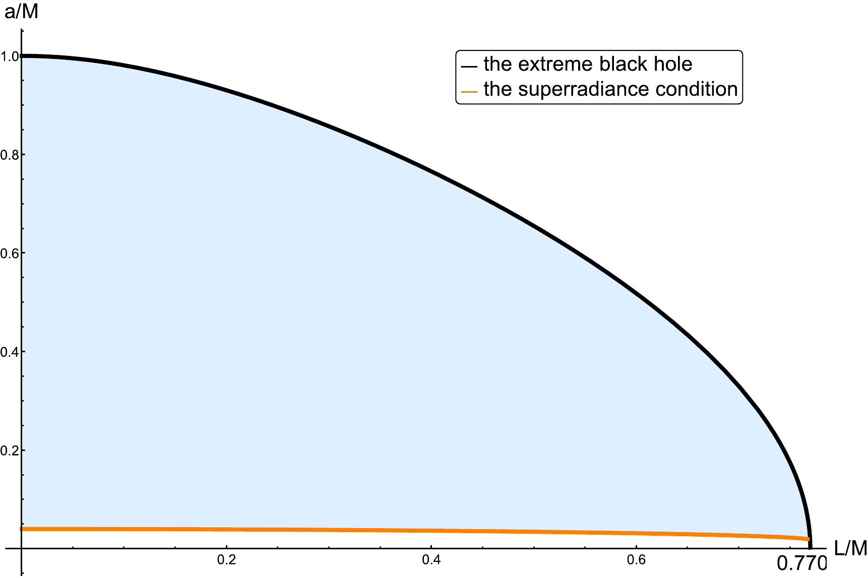
Figure 2. (color online) Relationship between the regularization parameter L and the rotation parameter a in the rotating Hayward black holes, where the abscissa is
$ L/M $ , the ordinate is$ a/M $ , and M represents the mass of the black hole. The black curve (depicted by Eqs. (82) and (83)) represents the extreme black hole, the orange curve (depicted by Eqs. (82) and (84)) is the lower bound for the occurrence of superradiance, and the blue area bounded by the two curves is the region of black hole parameters in which the superradiance can occur.Now, we discuss in detail how the regularization parameter L, together with the rotation parameter a, affects the evolution of amplitude of massive scalar particles in the quasi-bound state. Because we are concerned with the effects of the parameters a and L, we fix the particle mass to be
$ M\mu=0.01 $ in the following discussion. Because n affects only the constant term in Eq. (50), we take the fundamental order$ n=1 $ without loss of generality. According to Eq. (69), the critical condition that the superradiance phenomenon occurs is$ \frac{a}{\left(r_{\rm H}^+\right)^2+a^2}=\frac{0.01}{M}, $

(84) in which
$ r_{\rm H}^{+} $ is given by Eq. (82). Thus, Eqs. (82) and (84) give the orange curve in Fig. 2. Therefore, the blue area surrounded by the black and orange curves is the parameter region in which the superradiance can occur. Note that the intersection of the black and orange curves is$ (0.769, 0.018) $ , which indicates that there will be no superradiance effects when$ L>0.769M $ or$ a<0.018M $ , that is, the superradiance instability of quasi-bound particles and the superradiance scattering of free particles will not exist.In Fig. 3 we show the relationship between the imaginary part of frequency
$ \omega_{\rm I} $ and the regularization parameter L for quasi-bound state particles at the leading multipole number4 ($ l=1 $ ,$ m=1 $ ,$ n=1 $ ) when the rotation parameter a takes various values. We note that$ \omega_{\rm I} $ is positively correlated with the growth rate of the amplitude of quasi-bound state particles. It can be seen that the effect of L on$ \omega_{\rm I} $ is related to the value of a. When$ a<0.050M $ ,$ \omega_{\rm I} $ first increases and then decreases with an increase in L. This indicates that the growth rate of superradiance instability first increases and then decreases when L remains in the low rotation situation, i.e.,$ a<0.050M $ . Moreover, if$ a>0.050M $ ,$ \omega_{\rm I} $ monotonically decreases with an increase in L, which indicates that the growth rate of superradiance instability decreases with an increase in L. However,$ \omega_{\rm I} $ always increases monotonically with an increase in a for a fixed L. Thus, an increase in a always makes the superradiance instability grow very fast. In summary, the relationship between the growth rate of superradiance instability and L depends on the rotation parameter a, but the relationship between the growth rate of superradiance instability and a is always positively correlated for any fixed L.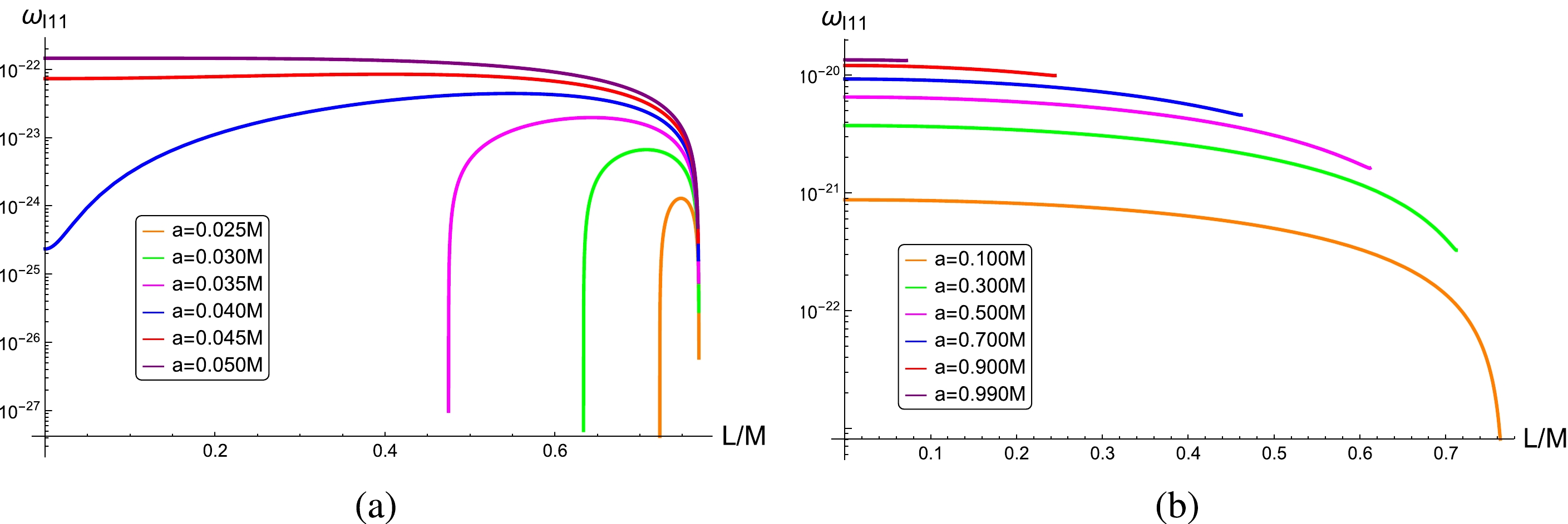
Figure 3. (color online) Relationship between the imaginary part of frequency
$ \omega_{\rm I} $ and the regularization parameter L for quasi-bound state particles at the leading multipole number ($ l=1 $ ,$ m=1 $ ,$ n=1 $ ) in the rotating Hayward black holes when the rotation parameter a takes various values, where diagram (a) corresponds to the case of$ 0.018M<a\le 0.050M $ , and diagram (b) corresponds to the case of$ 0.050M<a<1.000M $ .Next, we focus on how the regularization parameter L, together with the rotation parameter a, affects the superradiance amplification of massive scalar particles in the scattering process. Here, we fix the particle mass to be
$ M\mu=0.01 $ again and discuss the behavior of particles at the leading multipole number ($ l=1 $ ,$ m=1 $ ,$ n=1 $ ) in the background of a rotating Hayward black hole.Under the condition of a fixed regularization parameter L and rotation parameter a, the superradiance amplification has a peak when the particle frequency ω changes, which represents the maximum energy extraction efficiency. We note that such an efficiency is mainly affected by L and a. After analyzing the change of peaks with respect to L and a, we find that the change of peaks with respect to L is different in various intervals of a. Here, we call the change in each interval of a "one mode." We summarize four modes in the parameter region (see Fig. 2) where the superradiance effect can occur. The four modes are described in detail as follows.
1. The mode in the interval of
$ 0.018M<a<0.100M $ In this case, the peak value of superradiance magnification first increases and then decreases with an increase in L, and it finally has a very small increase when the rotating Hayward black hole approaches its extreme configuration. This shows that when L increases, the energy extraction efficiency of massive scalar particles scattered by the rotating Hayward black hole is initially higher but finally lower than that in the singular Kerr black hole (
$ L=0 $ ). In Fig. 4,$ a=0.050M $ is taken as an example, which is covered by the present interval$ 0.018M<a<0.100M $ . When L is in the range of$ 0<L\le 0.655M $ , the peak value of magnification increases if L is increasing, and it reaches the maximum value of$ 9.124\times 10^{-10} $ at$ L=0.655M $ . When L is in the range of$ 0.655M<L\le 0.768176M $ ,5 the peak value of magnification decreases if L is increasing, and it reaches the minimum value of$ 8.836\times 10^{-12} $ at$ L=0.768176M $ , where the rotating Hayward black hole is very close to its extreme configuration. When L is in the range of$ 0.768176M<L<0.768177M $ , the rotating Hayward black hole evolves to its final stage—the extreme configuration—and the peak rises with a slight uptick as the black hole approaches its extreme case.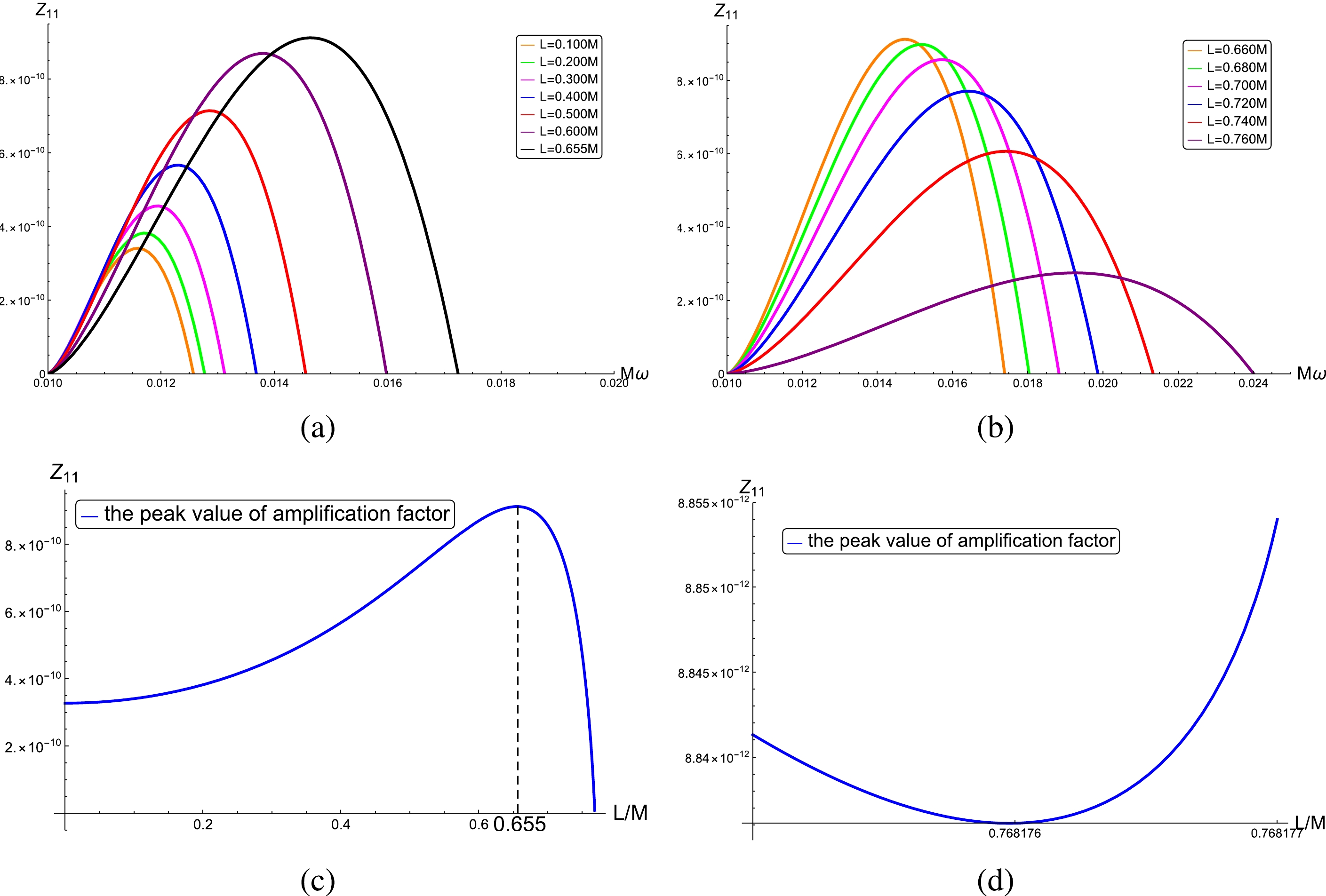
Figure 4. (color online) Amplification factor of massive scalar particles scattered by the rotating Hayward black hole computed via Eq. (68), where the parameters are set as follows:
$ M\mu=0.010 $ ,$ a=0.050M $ ,$ (l,m)=(1,1) $ , and a varying L. In diagram (a),$ 0<L\le 0.655M $ , and in diagram (b),$ 0.655M<L\le 0.768176M $ . Diagram (c) depicts the overall variation of the peak of the amplification factor with respect to L, and diagram (d) describes the behavior of the peak when the rotating Hayward black hole approaches its extreme configuration, i.e.,$ 0.768175M\le L < 0.768177M $ .2. The mode in the interval of
$ 0.100M<a<0.859M $ At first, the peak of the superradiance amplification factor decreases with an increase in L, and it reaches its lowest value when the rotating Hayward black hole approaches its near-extreme configuration. Then, the peak rises rapidly in the process of the black hole approaching its extreme configuration, but it does not exceed the peak value associated with the Kerr black hole (
$ L=0 $ ). This shows that the efficiency is the maximum for the massive scalar particles to extract energy from the Kerr black hole ($ L=0 $ ) in this interval of a and that the introduction of a regularization parameter (a non-vanishing L) will reduce this efficiency. In Fig. 5, we show the image of the peak of the amplification factor as a function of L for different values of a. As the rotation parameter increases, as shown in diagrams (a) to (d), the peak continuously rises in the process of the rotating Hayward black hole approaching its extreme configuration. In particular, the peak's order of magnitude increases with an increase in the rotation parameter. When the change in the order of magnitude caused by a is compared with that caused by L, we can see that the peak of the amplification factor is mainly affected by a rather than by L. In Fig. 6,$ a=0.800M $ is taken as an example, which belongs to the present mode, i.e.,$ 0.100M<a<0.859M $ . When L is in the range of$ 0<L\le 0.345M $ , the peak value of magnification decreases if L is increasing, and it reaches the minimum of$ 1.532\times10^{-4} $ at$ L=0.345M $ . Moreover, the peak value starts to increase again in the process of the rotating Hayward black hole approaching its extreme configuration, but it is still lower than that associated with the Kerr black hole, even if the rotating Hayward black hole arrives at its extreme. As a result, the peak value related to the Kerr black hole is the largest in the second mode of a-parameter intervals.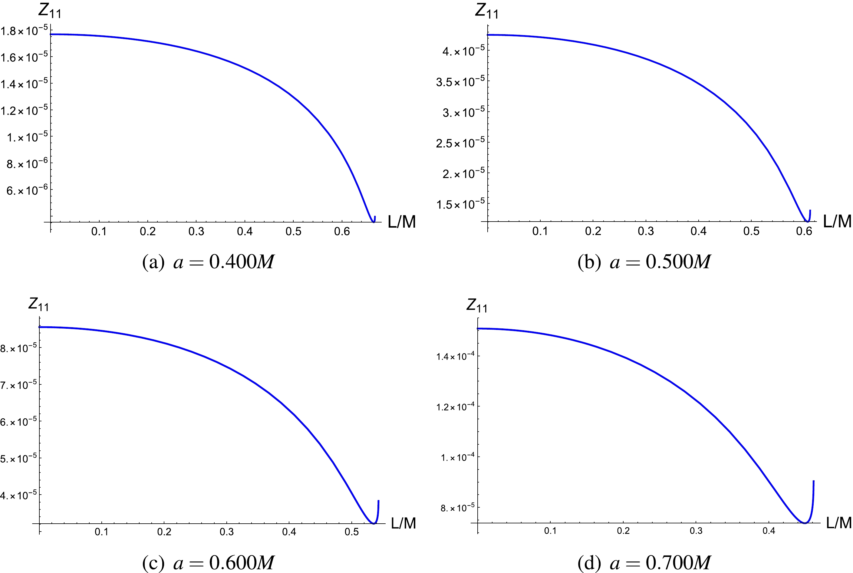
Figure 5. (color online) Relationship between the peak of the amplification factor and the regularization parameter L for the massive scalar particles scattered by the rotating Hayward black hole, where the parameters are set as follows:
$ M\mu=0.010 $ ,$ (l,m)=(1,1) $ , and a varying rotation parameter a.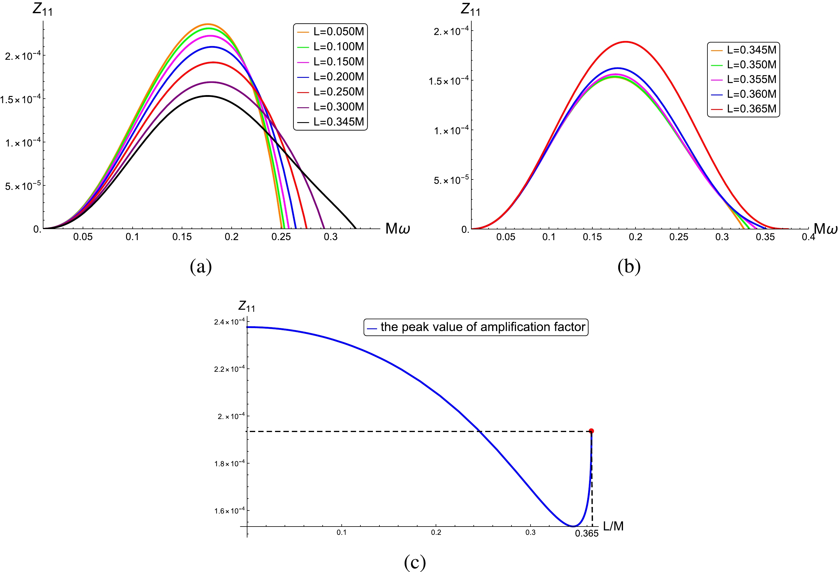
Figure 6. (color online) Amplification factor of massive scalar particles scattered by the rotating Hayward black hole computed via Eq. (68), where the parameters are set as follows:
$ M\mu=0.010 $ ,$ a=0.800M $ ,$ (l,m)=(1,1) $ , and a varying L. In diagram (a),$ 0<L\le 0.345M $ , and in diagram (b),$ 0.345M<L\le 0.365M $ . Diagram (c) depicts the overall variation of the peak of the amplification factor with respect to L.3. The mode in the interval of
$ 0.859M<a<0.963M $ In this mode, the variation of the peak of the superradiance amplification factor with respect to L is the same as that in the second mode. The main difference is that the peak is larger than that associated with the Kerr black hole when the rotating Hayward black hole is approaching its extreme configuration. This shows that when L increases, the efficiency for massive scalar particles to extract energy from the rotating Hayward black hole is initially lower but finally higher than that for the Kerr black hole (
$ L=0 $ ). In Fig. 7,$ a=0.900M $ is taken as an example, which belongs to the present mode, i.e.,$ 0.859M< a<0.963M $ . When$ L=0.245M $ , the rotating Hayward black hole reaches its extreme configuration, and the corresponding peak of the superradiance amplification factor reaches the maximum value of$ 3.967\times 10^{-4} $ , which is larger than that of$ 3.415\times 10^{-4} $ related to the Kerr black hole.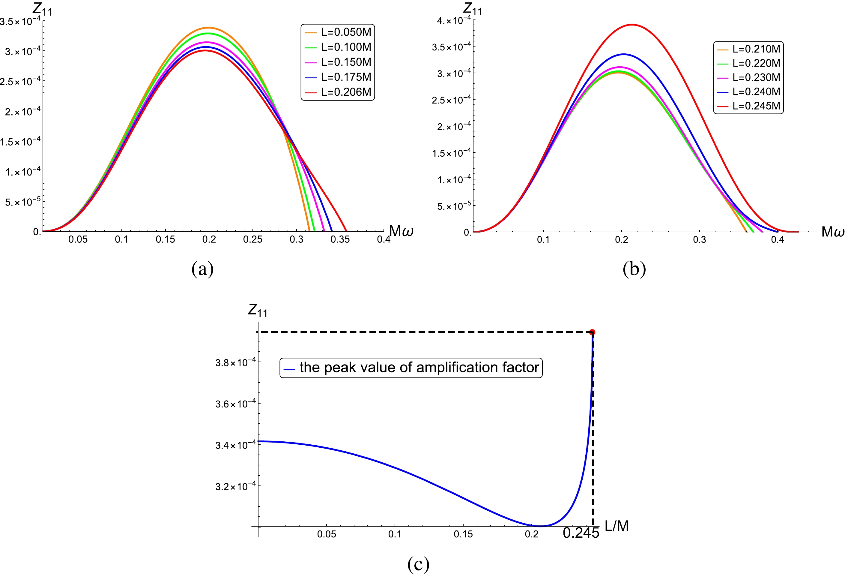
Figure 7. (color online) Amplification factor of massive scalar particles scattered by the rotating Hayward black hole computed by Eq. (68), where the parameters are set as follows:
$ M\mu=0.010 $ ,$ a=0.900M $ ,$ (l,m)=(1,1) $ , and a varying L. In diagram (a),$ 0<L\le 0.206M $ , and in diagram (b),$ 0.206M<L\le 0.245M $ . Diagram (c) depicts the overall variation of the peak of the amplification factor with respect to L.4. The mode in the interval of
$ 0.963M<a<M $ The peak of the superradiance amplification factor rises with an increase in L, and it reaches the maximum when the rotating Hayward black hole approaches its extreme configuration. This means that when L increases, the efficiency for massive scalar particles to extract energy from the rotating Hayward black hole is always higher than that for the Kerr black hole (
$ L=0 $ ). In Fig. 8,$ a=0.990M $ is taken as an example, which belongs to the present mode, i.e.,$ 0.963M<a<M $ . When$ L=0.070M $ , the rotating Hayward black hole reaches its extreme configuration, and the peak of the superradiance amplification factor reaches the maximum value of$ 7.904\times 10^{-4} $ , which is larger than that of$ 5.942\times 10^{-4} $ related to the Kerr black hole.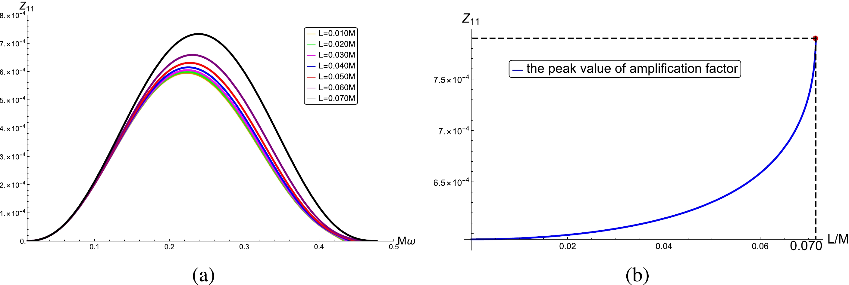
Figure 8. (color online) Amplification factor of massive scalar particles scattered by the rotating Hayward black hole computed via Eq. (68), where the parameters are set as follows:
$ M\mu=0.010 $ ,$ a=0.990M $ ,$ (l,m)=(1,1) $ , and$ 0<L\le 0.070M $ . Diagram (b) depicts the overall variation of the peak of the amplification factor with respect to L.From the above four modes, we can infer that the introduction of a regularization parameter L has both promotional and inhibitory effects on the efficiency of energy extraction and that whether the former or latter effect is dominant depends on the rotation parameter of the rotating Hayward black hole. Referring to the above discussions, we divide the values of the rotation parameter into four intervals: the low rotation interval (
$ 0.018M<a< 0.100M $ ), the middle rotation interval ($ 0.100M<a< 0.859M $ ), the high rotation interval ($ 0.859M<a< 0.963M $ ), and the near-extreme rotation interval ($ 0.963M< a<M $ ).In the low rotation interval, the introduction of L gives rise to two effects that are opposite to each other, i.e., the promotional and inhibitory effects, on the energy extraction efficiency, and whether the peak of the amplification factor related to the rotating Hayward black hole (
$ L\ne 0 $ ) is larger or smaller than that related to the Kerr black hole ($ L=0 $ ) depends on the competition of these two effects. When L begins to increase from zero, the promotional effect grows more quickly than the inhibitory effect, and finally the peak of the amplification factor reaches its maximum at a certain L. When L increases further, the promotional effect grows more slowly than the inhibitory effect; thus, the peak of the amplification factor begins to decline. When L reaches a certain threshold, the promotional effect is the same as the inhibitory effect, and the peak of the amplification factor is the same as that related to the Kerr black hole. After L exceeds this threshold, the inhibitory effect dominates, and the energy extraction efficiency becomes lower than that associated with the Kerr black hole. When L approaches the value at which the rotating Hayward black hole is close to its extreme configuration, the promotional effect grows more quickly than the inhibitory effect again; thus, there is a slight rise in the peak of the amplification factor. In summary, for the low rotation interval, the dominant role of the promotional effect is gradually replaced by the inhibitory effect when L increases, so that the energy extraction efficiency related to the rotating Hayward black hole is first higher and then lower than that related to the Kerr black hole.In the middle rotation interval, the inhibitory effect of L on the energy extraction efficiency is always greater than the promotional effect. When L increases from zero and reaches the value at which the rotating Hayward black hole is close to its extreme configuration, the promotional effect grows more quickly than the inhibitory effect; thus, the peak of the amplification factor will rise to a certain extent. Although the peak will rise higher for a larger rotation parameter a, it is still lower than that related to the Kerr black hole.
In the high rotation interval, the inhibitory effect of L on the energy extraction efficiency is initially greater than the promotional effect. When L begins to increase from zero, the inhibitory effect grows more quickly than the promotional effect, and finally the peak of the amplification factor reaches its minimum at a specific value of L. After L exceeds this specific value, the promotional effect grows more quickly than the inhibitory effect; thus, the peak of the amplification factor begins to rise and reaches its maximum value, at which the rotating Hayward black hole is close to its extreme configuration. This maximum value exceeds the peak related to the Kerr black hole.
In the near-extreme rotation interval, the promotional effect of L on the energy extraction efficiency is always greater than the inhibitory effect; thus, the peak of the amplification factor is always larger than that related to the Kerr black hole. When L begins to increase from zero, the promotional effect grows more quickly than the inhibitory effect, and finally the peak of the amplification factor reaches its maximum, at which the rotating Hayward black hole is close to its extreme configuration.
From what has been discussed above, we draw the following three conclusions:
● For massive scalar fields in the background of rotating Hayward black holes, the peak of the amplification factor is dominated by the rotation parameter a, not by the regularization parameter L, which plays only a secondary role.
● For four rotation parameter intervals, the influence of L on the peak of the amplification factor exhibits various situations. In short, there are four modes in which the energy extraction efficiency varies in accordance with the competition between the two parameters a and L.
● When a rotating Hayward black hole remains in its near-extreme configuration, the peak of the amplification factor always grows with an increase in L. Furthermore, a larger value of L indicates that the rotating Hayward black hole is closer to the extreme configuration.
-
After extending the static and spherically symmetric Bardeen black hole to the rotating and axially symmetric one that is still regular everywhere [16], we derive the equation that governs the event horizons of the rotating Bardeen black hole:
$ \left(r_{\rm H}^2+a^2\right)^2 \left(r_{\rm H}^2+g^2\right)^3-4 M^2r_{\rm H}^8=0. $

(85) This algebraic equation has two positive and real solutions
$ r_{\rm H}^- $ and$ r_{\rm H}^+ $ , which correspond to the inner and outer horizons, respectively. When the inner and outer horizons are equal, the black hole reaches its extreme configuration. The derivative of Eq. (85) with respect to$ r_{\rm H} $ gives rise to the equation that governs$ r_{\rm H}^{\rm ext} $ , i.e., the horizon of the extreme configuration:$ \begin{aligned}[b]& 2 \left(\left(r_{\rm H}^{\rm ext}\right)^2+a^2\right) \left(\left(r_{\rm H}^{\rm ext}\right)^2+g^2\right)^3\\ +& 3 \left(\left(r_{\rm H}^{\rm ext}\right)^2+a^2\right)^2 \left(\left(r_{\rm H}^{\rm ext}\right)^2+g^2\right)^2-16 M^2 \left(r_{\rm H}^{\rm ext}\right)^6=0, \end{aligned} $

(86) which, together with Eq. (85), gives the black curve in Fig. 9. The area surrounded by the black curve is just the parameter region where the black hole exists. As for the rotating Hayward black hole, we fix the particle mass to be
$ M\mu=0.01 $ for the rotating Bardeen black hole. According to Eq. (69), the critical condition that the superradiance phenomenon occurs has the same form as Eq. (84), in which$ r_{\rm H}^+ $ is determined by Eq. (85) instead of Eq. (82). That is, Eqs. (84) and (85) give the orange curve in Fig. 9. Therefore, the blue area surrounded by the black curve and the orange curve is the parameter region in which the superradiance can occur. Note that the intersection of the black and orange curves is$ (0.769,0.013) $ , which indicates that there will be no superradiance effect when$ g>0.769M $ or$ a<0.013M $ .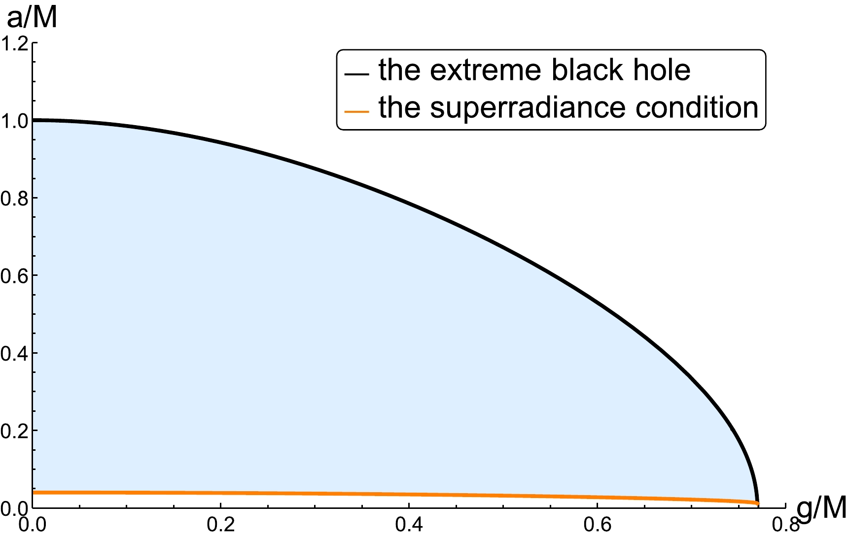
Figure 9. (color online) Relationship between the rotation parameter a and the magnetic charge g in rotating Bardeen black holes, where the abscissa is
$ g/M $ , the ordinate is$ a/M $ , and M represents the mass of the black hole. The black curve (given by Eqs. (85) and (86)) represents the extreme black hole, the orange curve (given by Eqs. (84) and (85)) is the lower bound for the occurrence of superradiance, and the blue area bounded by the two curves is the region of black hole parameters in which the superradiance can occur.Now, we discuss how the magnetic charge g, together with the rotation parameter a, affects the amplitude of a massive scalar particle in its quasi-bound state. In Fig. 10, we show the relationship between the imaginary part of frequency
$ \omega_{\rm I} $ for quasi-bound state particles at the leading multipole number ($ l=1 $ ,$ m=1 $ ,$ n=1 $ ) when the rotation parameter a takes various values. We note that$ \omega_{\rm I} $ is positively correlated with the growth rate of amplitude of quasi-bound state particles. It can be seen that the effect of g on$ \omega_{\rm I} $ is related to the value of a. When$ a<0.055M $ ,$ \omega_{\rm I} $ first increases and then decreases with an increase in g. This indicates that the growth rate of superradiance instability first increases and then decreases when g remains in the low rotation interval$ a<0.055M $ . Moreover, if$ a>0.055M $ ,$ \omega_{\rm I} $ monotonically decreases with an increase in g, which indicates that the growth rate of superradiance instability decreases with an increase in g. However,$ \omega_{\rm I} $ always increases monotonically with an increase in a for a fixed g. Thus, an increasing a also makes the superradiance instability grow very fast in the rotating Bardeen black hole. In summary, the relationship between the growth rate of superradiance instability and g depends on the rotation parameter a, but the relationship between the growth rate of superradiance instability and a is always positively correlated for any fixed g.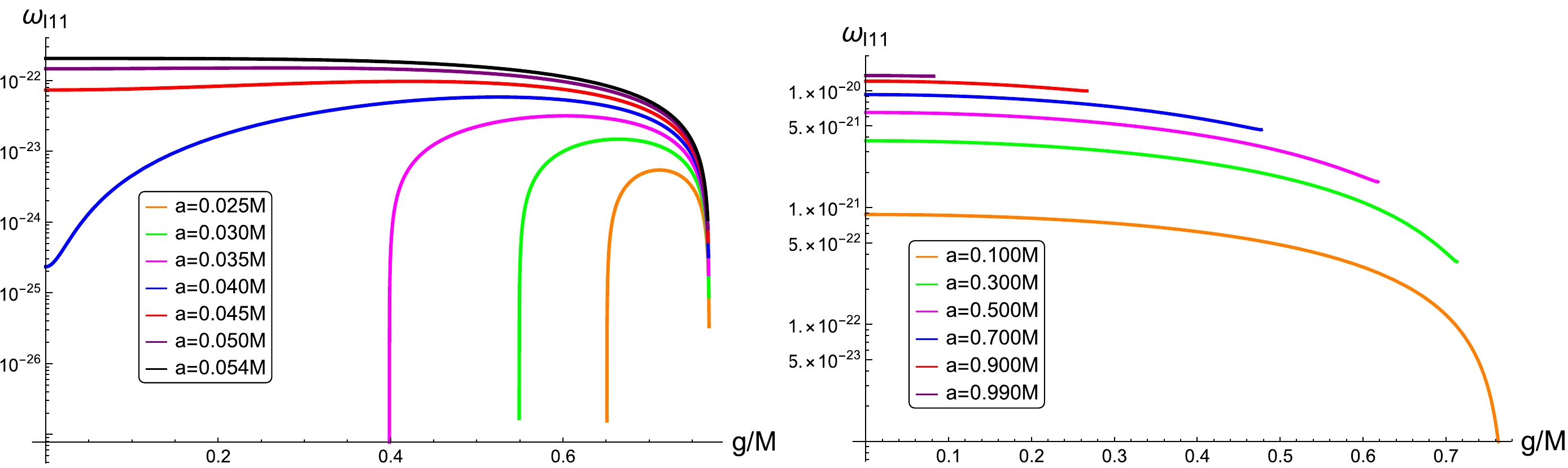
Figure 10. (color online) Relationship between the imaginary part of frequency
$ \omega_{\rm I} $ and the magnetic charge g for quasi-bound state particles that are scattered by rotating Bardeen black holes and are at the leading multipole number$ (l=1, m=1, n=1) $ when the rotation parameter a takes various values, where the left diagram corresponds to the case of$ 0.013M<a<0.055M $ , and the right diagram corresponds to the case of$ 0.055M<a<1.000M $ .Next, we focus on how the magnetic charge g, together with the rotation parameter a, affects the superradiance amplification of massive scalar particles. We discuss the behavior of particles still by setting
$ M\mu=0.010 $ at the leading multipole ($ l=1, m=1 $ ) in the background of a rotating Bardeen black hole. We also summarize four modes of the influence of g on the peak of the superradiance amplification factor when the rotation parameter a varies in the parameter region where the superradiance effect can occur. The four modes are analyzed in detail as follows.1. The mode in the interval of
$ 0.013M<a<0.246M $ The peak of the amplification factor first rises and then falls with an increase in the magnetic charge g.
This shows that the energy extraction efficiency of massive scalar particles scattered by the rotating Bardeen black hole is initially higher but finally lower than that of massive scalar particles scattered by the singular Kerr black hole (
$ g=0 $ ) when g increases. In particular, we note that the peak value will rise again when the rotating Bardeen black hole is close to its extreme configuration. In Fig. 11,$ a=0.100M $ is taken as an example. When g is in the range of$ 0<g\le0.545M $ , the peak value rises with an increase in g, and it reaches its maximum value of$ 5.310\times 10^{-8} $ at$ g=0.545M $ . Then, when g is in the range of$ 0.545M<g\le0.76325M $ , the peak value decreases with an increase in g, and it reaches its minimum value of$ 3.493\times 10^{-9} $ at$ g=0.76325M $ , where the rotating Bardeen black hole is very close to the extreme configuration. When g further increases to the range of$ 0.76325M< g\le0.76333M $ , the peak has a slight uptick as the black hole approaches the extreme configuration.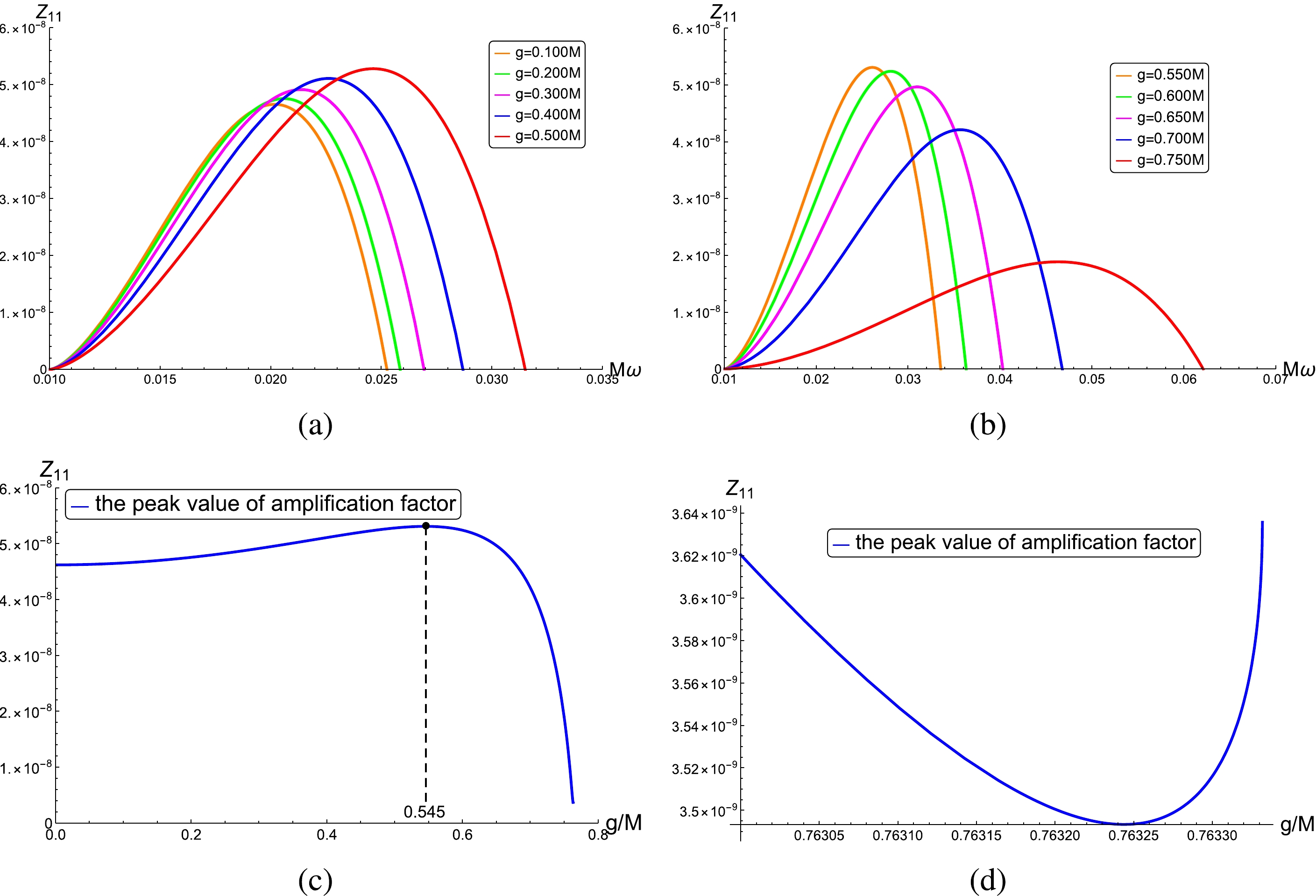
Figure 11. (color online) Amplification factor of massive scalar particles scattered by the rotating Bardeen black hole computed via Eq. (68), where the parameters are set as follows:
$ M\mu=0.010 $ ,$ a=0.100M $ ,$ (l,m)=(1,1) $ , and a varying g. In diagram (a),$ 0<g\le0.545M $ , and in diagram (b),$ 0.545M<g<0.76300M $ . Diagram (c) depicts the overall variation of the peak of the amplification factor with respect to g, and diagram (d) describes the behavior of the peak when the rotating Bardeen black hole approaches its near-extreme configuration,$ 0.76300M\le g < 0.76333M $ .2. The mode in the interval of
$ 0.246M<a<0.737M $ The peak value of the superradiance magnification falls monotonically when g increases from zero and reaches its minimum when g takes a certain range of values in which the rotating Bardeen black hole approaches its near-extreme configuration. When g increases further, the peak rises very rapidly, and it reaches its highest value, at which the rotating Bardeen black hole is in its extreme configuration. However, as shown in Fig. 12, the peak never exceeds the value associated with the Kerr black hole (
$ g=0 $ ) when a belongs to this mode. This shows that the efficiency is the maximum for a massive scalar particle to extract energy from the Kerr black hole ($ g=0 $ ) and that the introduction of the magnetic charge (a non-vanishing g) will reduce this efficiency. In particular, the order of magnitude of the peak increases with an increase in a. When the change in the order of magnitude caused by a is compared with that caused by g, we can see that the peak of the amplification factor is affected mainly by a rather than by g. In Fig. 13,$ a=0.700M $ is taken as an example. When g takes the range of$ 0<g\le 0.453M $ , the peak of the amplification factor falls with an increase in g, and it reaches its minimum value of$ 1.013\times10^{-4} $ at$ g=0.453M $ . Moreover, the peak starts to rise again when g increases further from$ 0.453M $ (this process means that the rotating Bardeen black hole is approaching to its extreme configuration), but it is still lower than that associated with the Kerr black hole, even if the rotating Bardeen black hole arrives at the extreme. As a result, the peak related to the Kerr black hole is the largest in the second mode of a-parameter intervals.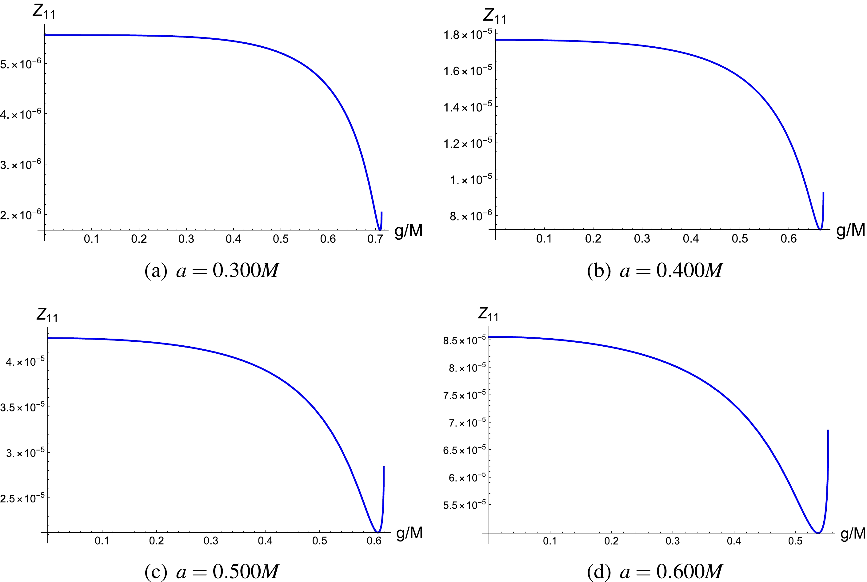
Figure 12. (color online) Relationship between the peak of the amplification factor and the magnetic charge g for the massive scalar particles scattered by the rotating Bardeen black hole, where the parameters are set as follows:
$ M\mu=0.010 $ ,$ (l,m)=(1,1) $ , and a varying rotation parameter a.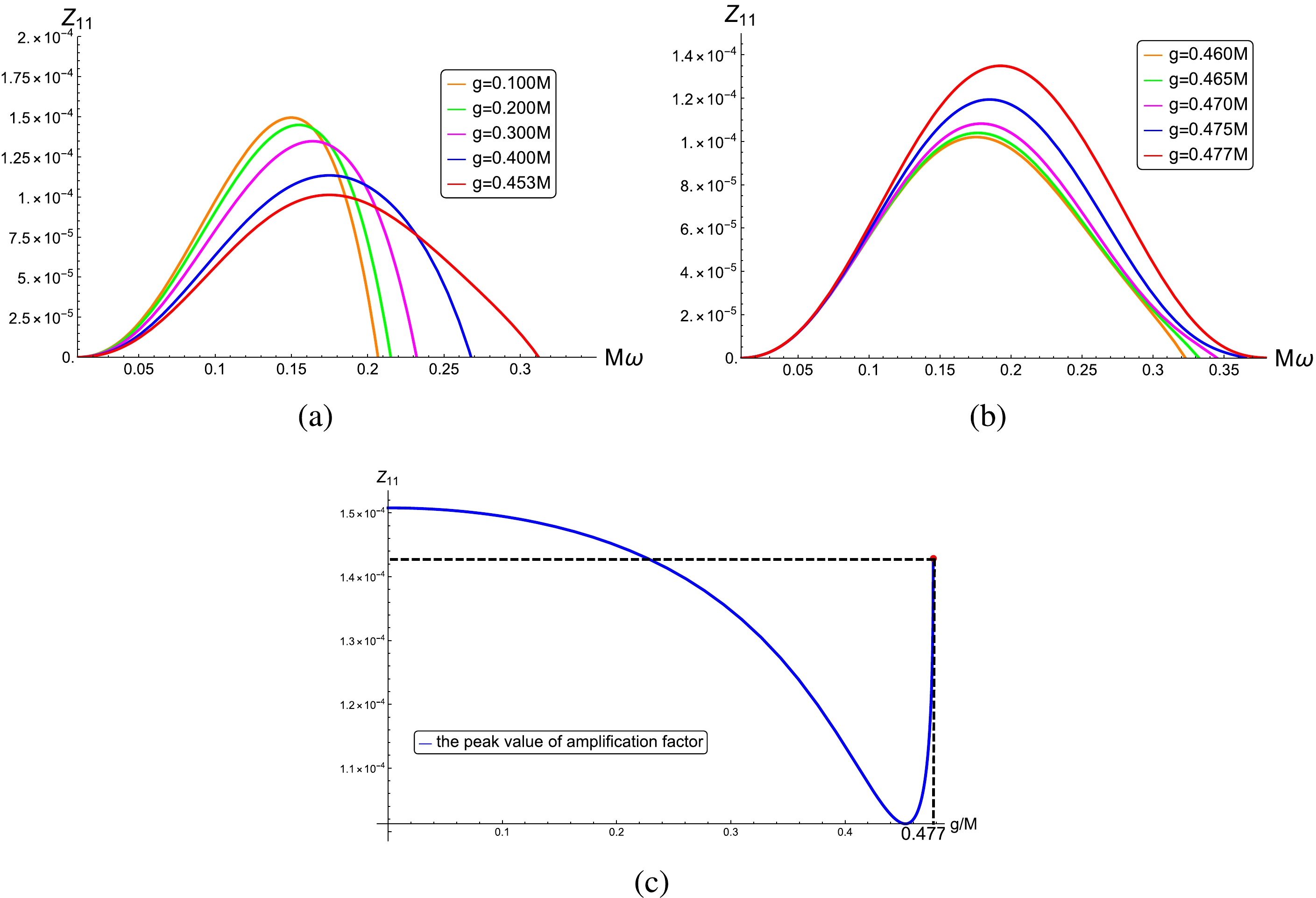
Figure 13. (color online) Amplification factor of massive scalar particles scattered by the rotating Bardeen black hole computed via Eq. (68), where the parameters are set as follows:
$ M\mu=0.010 $ ,$ a=0.700M $ ,$ (l,m)=(1,1) $ , and a varying g. In diagram (a),$ 0<g\le0.453M $ , and in diagram (b),$ 0.453M<g\le 0.477M $ . Diagram (c) depicts the overall variation of the peak of the amplification factor with respect to g.3. The mode in the interval of
$ 0.737M<a<0.947M $ The variation of the peak of the superradiance amplification factor with respect to g is the same as that in the second mode. The main difference is that the peak is larger than that associated with the Kerr black hole when the rotating Bardeen black hole is approaching its extreme configuration. This suggests that the effect of magnetic charges makes the efficiency of extracting energy from the rotating Bardeen black hole higher than that for the Kerr black hole. In Fig. 14,
$ a=0.800M $ is taken as an example. When$ g=0.385M $ , the rotating Bardeen black hole reaches its extreme configuration, and the peak reaches the maximum value of$ 2.721\times 10^{-4} $ , which is larger than that of$ 2.376\times 10^{-4} $ associated with the Kerr black hole.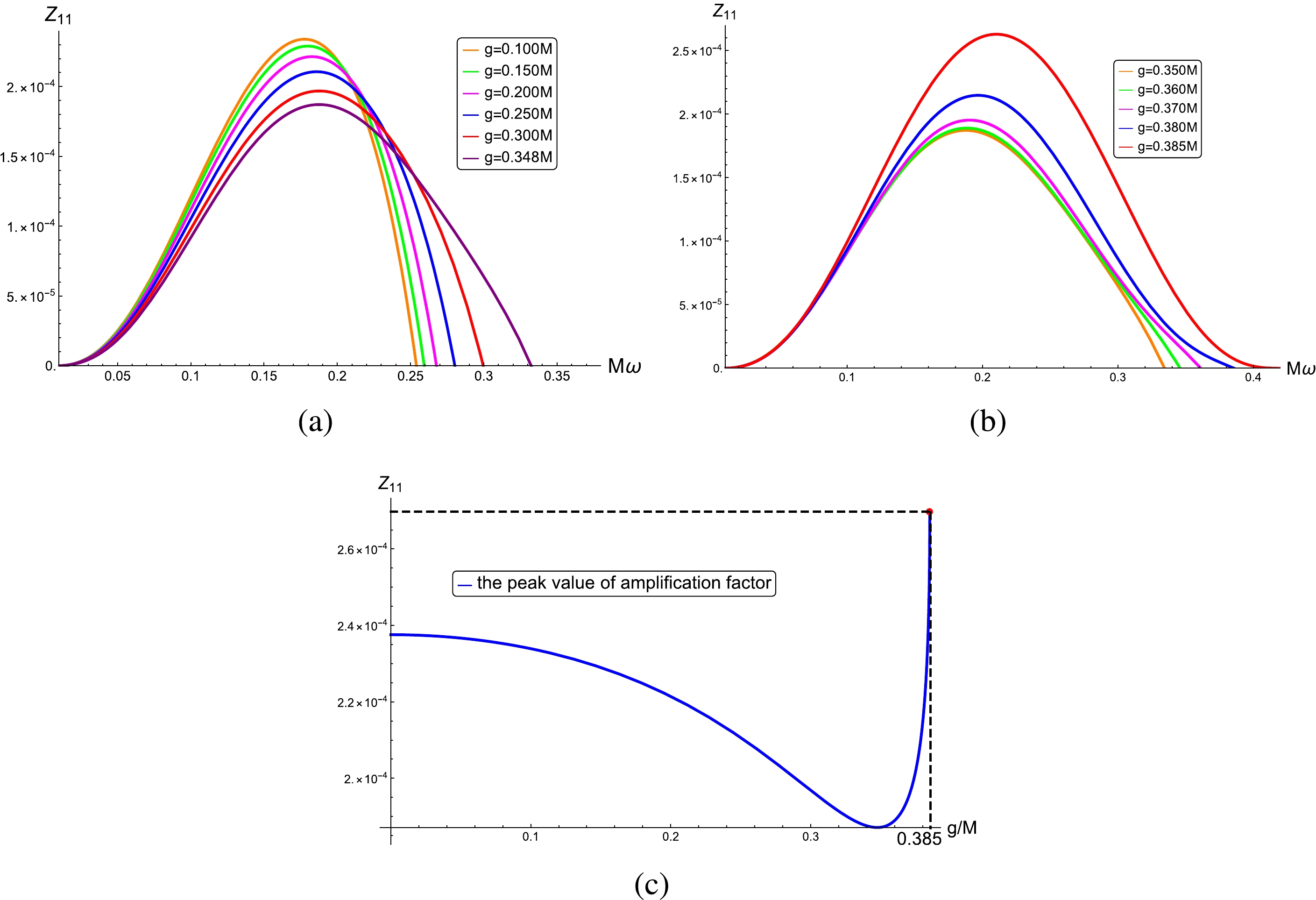
Figure 14. (color online) Amplification factor of massive scalar particles scattered by the rotating Bardeen black hole computed via Eq. (68), where the parameters are set as follows:
$ M\mu=0.010 $ ,$ a=0.800M $ ,$ (l,m)=(1,1) $ , and a varying g. In diagram (a),$ 0<g\le0.348M $ , and in diagram (b),$ 0.348M<g\le 0.385M $ . Diagram (c) depicts the overall variation of the peak of the amplification factor with respect to g.4. The mode in the interval of
$ 0.947M<a<M $ The peak rises monotonically with an increase in the magnetic charge, and it reaches its maximum when the rotating Bardeen black hole approaches its extreme configuration. This shows that the introduction of g makes the efficiency of energy extraction continuously increase. In Fig. 15,
$ a=0.990M $ is taken as an example. When$ g= 0.082M $ , the rotating Bardeen black hole reaches its extreme configuration, and the peak reaches its maximum value of$ 8.158\times 10^{-4} $ , which is larger than that of$ 5.942\times 10^{-4} $ related to the Kerr black hole.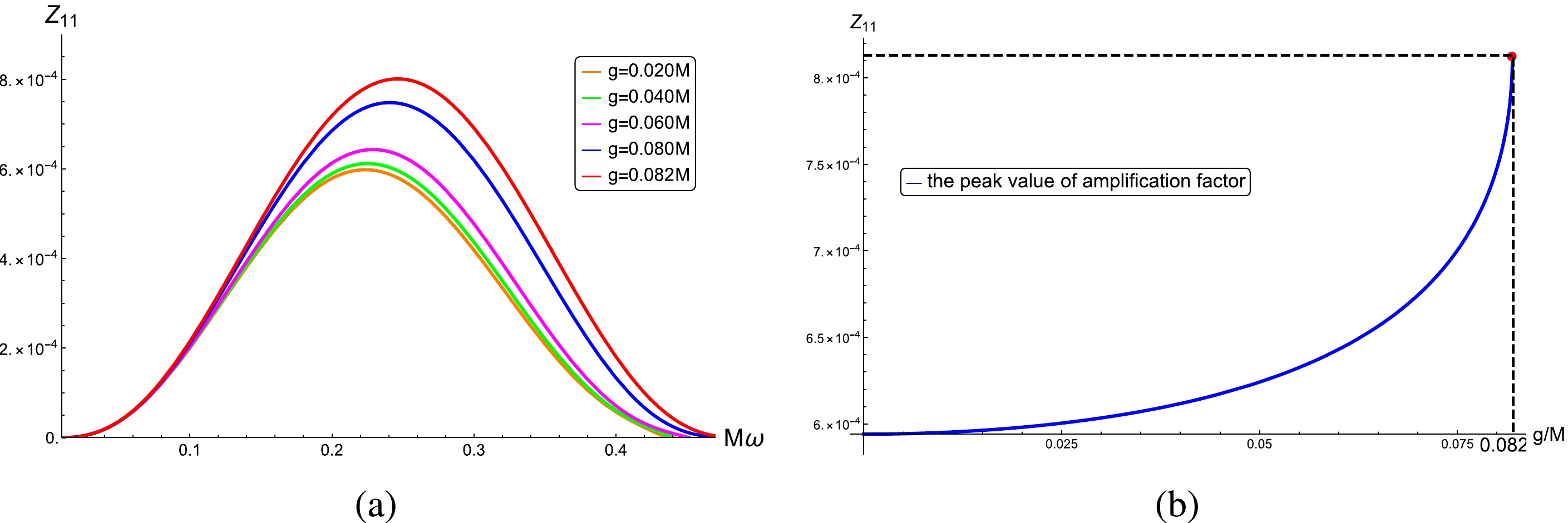
Figure 15. (color online) Amplification factor of massive scalar particles scattered by the rotating Bardeen black hole computed via Eq. (68), where the parameters are set as follows:
$ M\mu=0.010 $ ,$ a=0.990M $ ,$ (l,m)=(1,1) $ , and$ 0<g\le 0.082M $ . Diagram (b) depicts the overall variation of the peak of the amplification factor with respect to g.From the above four modes, we see that the rotation parameter can also be divided into four intervals for rotating Bardeen black holes: the low rotation interval (
$ 0.013M<a<0.246M $ ), the middle rotation interval ($ 0.246M<a<0.737M $ ), the high rotation interval ($ 0.737M<a<0.947M $ ), and the near-extreme rotation interval ($ 0.947M<a<M $ ). There also exist promotional and inhibitory effects of the regularization parameter g on the energy extraction efficiency in these four intervals. The promotional and inhibitory effects are consistent with those in the rotating Hayward black hole.Thus, we draw the following three conclusions:
● In the background of rotating Bardeen black holes, the peak of the amplification factor of massive scalar fields is dominated by the rotation parameter a, not by the magnetic charge g, which plays only a secondary role.
● For four rotation parameter intervals, the influence of g on the peak of the amplification factor exhibits various situations. In short, there are four modes in which the energy extraction efficiency varies in accordance with the competition between the two parameters a and g.
● When the rotating Bardeen black hole remains in its near-extreme configuration, the peak of the amplification factor always rises with an increase in g. Furthermore, a larger value of g indicates that the rotating Bardeen black hole is closer to the extreme configuration.
-
First, we review the rotating regular black holes constructed by the modified NJA and give the field equations satisfied by massive scalar particles in the background of such black holes. Then, for a scalar particle with a small mass, we calculate analytically the eigenfrequency of superradiance instability in its quasi-bound state and the superradiance amplification factor in its free state using the asymptotic matching method. For two specific models, i.e., the rotating Hayward black hole and the rotating Bardeen black hole, we analyze how the regularization parameter and rotation parameter affect the eigenfrequency and the amplification factor. Our main conclusions are summarized as follows.
● We provide the condition that the superradiance instability can occur for a scalar particle with a small mass when it is in its quasi-bound state; see Eq. (52). In addition, we give the condition the superradiance amplification can appear for a scalar particle with a small mass when it is in its free state; see Eq. (69). Comparing the two conditions, we can see that the two phenomena, i.e., the superradiance instability and superradiance amplification, are closely related. In fact, they occur or do not occur simultaneously.
● For the two specific models, i.e., the rotating Hayward and rotating Bardeen black holes, we find two modes for the growth of superradiance instability and four modes for the energy extraction of superradiance amplification. These modes depend on the competition between the regularization parameter and the rotation parameter in each model. In particular, we notice that the behaviors of superradiance instability and superradiance amplification are almost the same in the two models, which is natural because the regularization parameter plays the same role in each model.
In general, the static and spherically symmetric regular black holes can be divided [43] into four classes, where the Hayward and Bardeen black holes belong to the first class. In this class, every regular black hole contains a de Sitter-like core and has two horizons or one overlapped horizon at least, and its causal structure can be depicted by the Carter-Penrose diagram that is similar to that of a Reissner-Nordström black hole. However, the singularity avoidance in the Bardeen black hole can be understood by a mechanism called topology change [44, 45], that is, the Bardeen black hole has a topology different from that of the Reissner-Nordström black hole. Inspired by the classification of regular black holes and the mechanism of topology change, we plan to investigate the superradiance related effects for the rotating counterparts of the other three classes of regular black holes and explain their superradiance features by analyzing the topology of these black holes in our future work.
-
The authors would like to thank the anonymous referees for their helpful comments that improved this work greatly.
-
First, we solve the eigenfrequency according to Eq. (47). Because
$ \delta \nu $ is complex, with its real part$ \delta\nu_{\rm R} $ and imaginary part$ \delta\nu_{\rm I} $ , we rewrite Eq. (47) as$ \begin{aligned}[b] \mu^2-\omega^2 &=\frac{A^2\mu^4}{4(l+n+1+\delta\nu_{\rm R}+{\rm i}\delta\nu_{\rm I})^2}\\ &=\frac{A^2\mu^4(l+n+1+\delta\nu_{\rm R}-{\rm i}\delta\nu_{\rm I})^2}{4[(l+n+1+\delta\nu_{\rm R})^2+\delta\nu_{\rm I}^2]^2}.\\ \end{aligned}\tag{A1} $

Because the modulus of
$ \delta\nu $ is far smaller than 1, which indicates that both$ |\delta\nu_{\rm R}| $ and$ |\delta\nu_{\rm I}| $ are far smaller than 1, the above equation can be approximated as$ \begin{aligned}[b] \mu^2-\omega^2&\approx \frac{A^2\mu^4(l+n+1+\delta\nu_{\rm R}-{\rm i}\delta\nu_{\rm I})^2}{4(l+n+1+\delta\nu_{\rm R})^4}\\ &\approx \frac{A^2\mu^4}{4(l+n+1+\delta\nu_{\rm R})^2}-\frac{{\rm i}A^2\mu^4(l+n+1+\delta\nu_{\rm R})\delta\nu_{\rm I}}{2(l+n+1+\delta\nu_{\rm R})^4}\\ &\approx \frac{A^2\mu^4}{4(l+n+1)^2}-\frac{{\rm i}A^2\mu^4}{2(l+n+1)^3}\delta\nu_{\rm I}. \end{aligned}\tag{A2} $

Considering
$\mu^2-\omega^2=\mu^2-\omega_{\rm R}^2+\omega_{\rm I}^2-2{\rm i}\omega_{\rm R}\omega_{\rm I}$ and the slow change approximation$ \omega_{\rm R}\gg\omega_{\rm I} $ , we obtain from the above equation$ \mu^2-\omega_{\rm R}^2\approx \frac{A^2\mu^4}{4(l+n+1)^2}, \tag{A3}$

and
$ \omega_{\rm R}\omega_{\rm I}\approx\frac{A^2\mu^4}{4(l+n+1)^3}\delta\nu_{\rm I}. \tag{A4}$

Again, considering
$ \mu A\ll 1 $ (see Eq. (26) and the relevant explanation), we derive the approximate real part of the eigenfrequency from Eq. (A3):$ \omega_{\rm R} \approx \mu\left[1-\frac{A^2\mu^2}{8(l+n+1)^2}\right], \tag{A5}$

from which we deduce
$ \omega_{\rm R}<\mu $ , and the second term is far smaller than the first one, i.e.,$ \dfrac{A^2\mu^2}{8(l+n+1)^2}\ll 1 $ . Note that this inequality ($ \omega_{\rm R}<\mu $ ) means that the massive scalar particle remains in a quasi-bound state. By substituting Eq. (A5) into Eq. (A4), we obtain the approximate imaginary part of the eigenfrequency:$ \omega_{\rm I} \approx \frac{A^2\mu^3}{4(l+n+1)^3}\left[1+\frac{A^2\mu^2}{8(l+n+1)^2}\right]\delta\nu_{\rm I}. \tag{A6} $

Next, we need to derive
$ \delta\nu_{\rm I} $ from Eq. (46), in which the quantities k and P should be dealt with; for the definitions of k and P, see Eqs. (28) and (38), respectively.According to Eq. (28), k is complex and can be expressed as
$k=k_{\rm R}+{\rm i}k_{\rm I}$ ; thus, we obtain the following results up to their respective leading orders by using Eqs. (A5) and (A6):$ k_{\rm R}^2-k_{\rm I}^2=\mu^2-\omega_{\rm R}^2+\omega_{\rm I}^2\approx\frac{A^2\mu^4}{4(l+n+1)^2}\equiv C,\tag{A7} $

$ k_{\rm R}k_{\rm I}=-\omega_{\rm R}\omega_{\rm I}\approx-\frac{A^2\mu^4}{4(l+n+1)^3}\delta\nu_{\rm I}\equiv D. \tag{A8} $

Note that
$ C\gg |D| $ due to$ |\delta\nu_{\rm I}|\ll 1 $ . By solving Eqs. (A7) and (A8), we work out the real and imaginary parts of k approximately:$ k_{\rm R}^2\approx C, \tag{A9} $

$ k_{\rm I}^2\approx\frac{D^2}{C}. \tag{A10}$

Because
$ C\gg |D| $ , we deduce$ |k_{\rm R}|\gg |k_{\rm I}|, \tag{A11} $

which will be used to distinguish whether
$ k_{\rm R} $ or$ k_{\rm I} $ gives the main contribution to$ \delta\nu_{\rm I} $ in Eq. (46).We then turn to P. According to Eq. (38), P is complex, with its real part
$ P_{\rm R} $ and imaginary part$ P_{\rm I} $ . Consider the numerator of Eq. (38): the first term is far larger than the absolute value of the real part of the second term, because our approximations are$ \mu M\ll 1 $ and$ |\omega| M\ll 1 $ , which gives rise to$ P_{\rm R}\gg |P_{\rm I}|. \tag{A12} $

As a result, the main contribution to
$ \delta\nu_{\rm I} $ comes from the product of$ |k_{\rm R}| $ and$ P_{\rm R} $ according to Eqs. (46), (A11), and (A12).By using Eqs. (A7) and (A9), we obtain
$ k_{\rm R}\approx\frac{|A|\mu^2}{2(l+n+1)}, \tag{A13}$

where we have taken
$ k_{\rm R}>0 $ in order to ensure that x defined by Eq. (30) does not reverse the direction of r. If the direction of r were reversed, the directions of incoming and outgoing waves at two boundaries would be reversed, which would lead to inconvenience. Moreover, we compute$ P_{\rm R} $ in terms of Eqs. (38) and (A5):$ P_{\rm R}\approx\frac{ma-2\mu f(r_{\rm H}^+)}{2r_{\rm H}^+-2f'(r_{\rm H}^+)},\tag{A14} $

where we have ignored the second term in Eq. (A5), i.e., we have taken
$ \omega_{\rm R}\approx \mu $ . Similarly, we can also ignore the second term in Eq. (A6) and arrive at Eq. (49).By substituting Eqs. (A11)–(A14) into Eq. (46), we compute
$ \delta\nu_{\rm I} $ . By substituting this$ \delta\nu_{\rm I} $ into Eq. (49), we finally derive Eq. (50), which gives the imaginary part of the eigenfrequency.
Superradiance of massive scalar particles around rotating regular black holes
- Received Date: 2023-03-12
- Available Online: 2023-07-15
Abstract: Regular black holes, as part of an important attempt to eliminate the singularities in general relativity, have been of wide concern. Because the superradiance associated with rotating regular black holes plays an indispensable role in black hole physics, we calculate the superradiance related effects, i.e., the superradiance instability and the energy extraction efficiency, for a scalar particle with a small mass around a rotating regular black hole, where the rotating regular black hole is constructed by the modified Newman-Janis algorithm. We analytically give the eigenfrequency associated with instability and the amplification factor associated with energy extraction. For two specific models, i.e., the rotating Hayward and Bardeen black holes, we investigate how their regularization parameters affect the growth of instability and the efficiency of energy extraction from the two rotating regular black holes. We find that the regularization parameters give rise to different modes of the superradiance instability and the energy extraction when the rotation parameters vary. There are two modes for the growth of superradiance instability and four modes for the energy extraction. Our results show the diversity of superradiance in the competition between the regularization parameter and the rotation parameter for rotating regular black holes.


 DownLoad: