


 Abstract
 HTML
HTML Reference
 Related
 PDF
PDF


-
It is well known that lepton flavor violating (LFV) decays, such as
$ l_1\rightarrow l_2\gamma $ ,$ l_1\rightarrow 3l_2 $ ,$ \mu-e $ conversion,$ h\rightarrow l_1 l_2 $ , and$ \tau \rightarrow Pl_1 $ , are strongly suppressed by small masses of neutrinos in the standard model (SM), in which the neutrino oscillations (the masses and the mixing) are accommodated. In the SM with three massive neutrinos, the predicted branching ratios (BRs) of the LFV decays of the vector meson V are under$ 10^{-50} $ [1], and this is far below the current experimental sentivity. Nevertheless, in many new physics scenarios beyond the SM, the branching ratios of the LFV decays can be adjusted to be within the current experimental range; this is the case for the grand unified models [2−4], the two Higgs doublet models [5], the supersymmetric models [6], and the left-right symmetry models [7−9]. The results show that, in various SM extensions, the predicted BR$ (V\rightarrow l_1 l_2) $ can be within the range of the current or future experiments [1, 10−15]. The LFV decays of neutral vector mesons can also be studied in a model-independent manner [16−22], which can be used to obtain the constraints on the Wilson coefficients.Using a sample of about 10 billion
$ J/\psi $ events collected by the BESIII detector [23, 24], the BESIII collaboration reported their results for the LFV decays of$ J/\psi $ . The upper limits on BR$ (J/\psi\rightarrow e\mu) $ and BR$ (J/\psi\rightarrow e\tau) $ were$ 4.5\times 10^{-9} $ and$ 7.5\times 10^{-8} $ at the 90% confidence level (CL), improving over the previous limits by one and two orders of magnitude [25, 26], respectively. Using the collected 158 million$ \Upsilon(2S) $ events, the LFV decays of the neutral vector meson$ \Upsilon(1S) $ have been detected at the Belle detector at the KEKB$ e^+e^- $ collider [27]. The estimated upper limit on the BR of$ \Upsilon(1S)\rightarrow \mu\tau $ was$ 2.7\times 10^{-6} $ , which is 2.3 times more stringent than the previous result [28]. The Belle collaboration also performed the first search for$ \Upsilon(1S)\rightarrow e\mu $ and$ \Upsilon(1S)\rightarrow e\tau $ and the estimated upper limits were$ 3.9\times 10^{-7} $ and$ 2.7\times 10^{-6} $ , respectively. Using 118 million$ \Upsilon(3S) $ samples collected by the BABAR detector at the PEP-II collider at SLAC, the BABAR collaboration set the upper limit on the LFV decay BR$ (\Upsilon(3S)\rightarrow e\mu) $ at$ 3.6\times 10^{-7} $ , at the 90% CL [29]. In Table 1, we provide a summary of the current limits on the LFV decays of the neutral vector meson V (V =$ J/\psi $ ,$ \Upsilon(nS) $ , ϕ).Decay Limit Experiment Decay Limit Experiment $ J/\psi\rightarrow e\mu $ 

$ 4.5\times 10^{-9} $ 

BESIII (2022)[23] $ J/\psi\rightarrow e\tau $ 

$ 7.5\times 10^{-8} $ 

BESIII (2021)[24] $ J/\psi\rightarrow \mu\tau $ 

$ 2.0\times 10^{-6} $ 

BES (2004)[26] $ \Upsilon(1S)\rightarrow e\mu $ 

$ 3.9\times 10^{-7} $ 

BELLE (2022)[27] $ \Upsilon(1S)\rightarrow e\tau $ 

$ 2.7\times 10^{-6} $ 

BELLE (2022)[27] $ \Upsilon(1S)\rightarrow \mu\tau $ 

$ 2.7\times 10^{-6} $ 

BELLE (2022)[27] $ \Upsilon(2S)\rightarrow e\tau $ 

$ 3.2\times 10^{-6} $ 

BABAR (2010)[30] $ \Upsilon(2S)\rightarrow \mu\tau $ 

$ 3.3\times 10^{-6} $ 

BABAR (2010)[30] $ \Upsilon(3S)\rightarrow e\mu $ 

$ 3.6\times 10^{-7} $ 

BABAR (2022)[29] $ \Upsilon(3S)\rightarrow \mu\tau $ 

$ 3.1\times 10^{-6} $ 

BABAR (2010)[30] $ \Upsilon(3S)\rightarrow e\tau $ 

$ 4.2\times 10^{-6} $ 

BABAR (2010)[30] $ \phi\rightarrow e\mu $ 

$ 2\times 10^{-6} $ 

SND (2010)[31] Table 1. Current experimental limits on the LFV decays of neutral vector mesons.
In the present work, we analyze the LFV decays
$ V\rightarrow l_1 l_2 $ in a model that contains the continuous R-symmetry [32, 33] and is called the minimal R-symmetric supersymmetric standard model (MRSSM) [34]. The gauge symmetry of the MRSSM is the same as those of the SM and MSSM. R-symmetry forbids Majorana gaugino masses, and the MRSSM contains Dirac gauginos and the gauge/gaugino sector is an N = 2 supersymmetric theory. In the MRSSM, the μ term, A terms and the left-right mixings in the squark and slepton mass matrices, which usually exist in the MSSM, are also absent. In the MSSM there is a tanβ-enhancement for the muon anomalous magnetic dipole moment$ a_\mu $ [35, 36] and a similar enhancement for the predictions of BR$ (\mu\rightarrow e \gamma) $ and CR$ (\mu-e,nucleus) $ [37]. However, the tanβ-enhancement for these observables does not exist in the MRSSM since there are no Majorana gaugino masses and no μ term [38]. The branching ratios of the LFV processes are affected by the off-diagonal inputs of the matrices$ m_l^2 $ and$ m_r^2 $ . Several references to the phenomenology of the MRSSM are provided [38−56].A brief introduction to the MRSSM is provided in Sec. II, and the notation for the operators and their corresponding Wilson coefficients are also given in that section. The numerical comparison of the different models is described in Sec. III. Section IV lists our conclusions.
-
In this section, we firstly provide a simple introduction to the MRSSM. Similar to the SM and MSSM, the gauge symmetry of the MRSSM is
$S U(3)_C\times S U(2)_L\times U(1)_Y$ . The spectrum of fields in the MRSSM contains the standard MSSM matter, the Higgs and gauge superfields augmented by chiral adjoints$ \hat{S} $ ,$ \hat{T} $ ,$ \hat{\cal O} $ and two R-Higgs iso-doublets. The R-charges of the superfields and the corresponding bosonic and fermionic components in the MRSSM are given in Table 2. The most general form of the superpotential in the MRSSM takes the form of Ref. [39]Field Superfield R-charge Boson R-charge Fermion R-charge Gauge vector $ \hat{g} $ ,

$ \hat{W} $ ,

$ \hat{B} $ 

0 g,W,B 0 $ \tilde{g} $ ,

$ \tilde{W} $ ,

$ \tilde{B} $ 

$ + $ 1

Matter $ \hat{l} $ ,

$ \hat{e} $ 

$ + $ 1

$ \tilde{l} $ ,

$ \tilde{e}^*_R $ 

$ + $ 1

l, $ e^*_R $ 

0 $ \hat{q} $ ,

$ {\hat{d}} $ ,

$ {\hat{u}} $ 

$ + $ 1

$ \tilde{q} $ ,

$ {\tilde{d}}^*_R $ ,

$ {\tilde{u}}^*_R $ 

$ + $ 1

q, $ d^*_R $ ,

$ u^*_R $ 

0 H-Higgs $ {\hat{H}}_{d,u} $ 

0 $ H_{d,u} $ 

0 $ {\tilde{H}}_{d,u} $ 

$ - $ 1

R-Higgs $ {\hat{R}}_{d,u} $ 

$ + $ 2

$ R_{d,u} $ 

$ + $ 2

$ {\tilde{R}}_{d,u} $ 

$ + $ 1

Adjoint chiral $ \hat{S} $ ,

$ \hat{T} $ ,

$ \hat{\cal O} $ 

0 S,T,O 0 $ \tilde{S} $ ,

$ \tilde{T} $ ,

$ \tilde{O} $ 

$ - $ 1

Table 2. The field content of the MRSSM.
$ \begin{aligned}[b] \mathcal{W}_{\rm MRSSM}=&\Lambda_d \hat{R}_d\cdot \hat{T}\hat{H}_d+\Lambda_u \hat{R}_u\cdot\hat{T}\hat{H}_u\\&+\lambda_d\hat{S}\hat{R}_d\cdot\hat{H}_d+\lambda_u\hat{S} \hat{R}_u\cdot\hat{H}_u\\ &-Y_d\hat{d}\hat{q}\cdot\hat{H}_d-Y_e\hat{e}\hat{l}\cdot\hat{H}_d\\&+Y_u\hat{u}\hat{q}\cdot\hat{H}_u+\mu_d\hat{R}_d\cdot \hat{H}_d+\mu_u \hat{R}_u\cdot \hat{H}_u, \end{aligned} $

(1) where the dot '
$ \cdot $ ' refers to an$S U(2)$ contraction with the Levi-Civita tensor, the MSSM-like Higgs weak iso-doublets are$ \hat{H}_u $ and$ \hat{H}_d $ , the R-charged Higgs$S U(2)_L$ doublets are$ \hat{R}_u $ and$ \hat{R}_d $ , and$ \mu_u $ and$ \mu_d $ stand for the Dirac higgsino mass parameters.$ Y_e $ ,$ Y_u $ and$ Y_d $ stand for the Yukawa couplings of a charged lepton, up quarks and down quarks, respectively.$ \lambda_{u,d} $ and$ \Lambda_{u,d} $ stand for the Yukawa-like trilinear terms that involve the singlet$ \hat{S} $ and triplet$ \hat{T} $ , and the triplet$ \hat{T} $ takes the form of$ \begin{eqnarray} \hat{T}=\left(\begin{array}{cc} \dfrac{\hat{T}^{0}}{\sqrt{2}} &\hat{T}^+ \\ \hat{T}^- &-\dfrac{\hat{T}^{0}}{\sqrt{2}}\end{array} \right). \end{eqnarray} $

For the phenomenological studies, we take the soft breaking scalar mass terms [39]
$ \begin{aligned}[b] V_{SB,S} =& (B_\mu(H^-_{d}H^+_{u}-H^{0}_{d}H^{0}_{u})+h.c.)\\&+m^{2}_{H_{u}}(|H^{0}_{u}|^{2}+|H^+_{u}|^{2})+m^{2}_{H_{d}}(|H^{0}_{d}|^{2}+|H^-_{d}|^{2})\\ &+m^{2}_{T}(|T^{0}|^{2}+|T^-|^{2}+|T^+|^{2})\\&+m^{2}_{R_{u}}(|R^{0}_{u}|^{2}+|R^-_{u}|^{2})+m^{2}_{R_{d}}(|R^{0}_{d}|^{2}+|R^+_{d}|^{2})\\ &+\tilde{u}^{\ast}_{L,i} m_{q,{i j}}^{2} \tilde{u}_{L,j}+\tilde{u}^{\ast}_{R,i} m_{u,{i j}}^{2} \tilde{u}_{R,j}+\tilde{d}^{\ast}_{L,i} m_{q,{i j}}^{2} \tilde{d}_{L,j}\\&+\tilde{d}^{\ast}_{R,i}m_{d,{i j}}^{2}\tilde{d}_{R,j}+\tilde{\nu}^{\ast}_{L,i} m_{l,{i j}}^{2} \tilde{\nu}_{L,j}\\ &+\tilde{e}^{\ast}_{L,i}m_{l,{i j}}^{2}\tilde{e}_{L,j}+\tilde{e}^{\ast}_{R,{i}} m_{r,{i j}}^{2}\tilde{e}_{R,{j}}+m^{2}_{S}|S|^{2}+ m^{2}_{O}|O|^{2}. \end{aligned} $

(2) Due to the R-symmetry, the trilinear terms that contain the interaction between the slepton/squark and the Higgs boson are absent. The couplings involving the auxiliary D-fields to the adjoint scalars and the Dirac gaugino mass terms are included in the soft break terms, given by
$ \begin{aligned}[b] V_{SB,DG}=&M^{W}_{D}(\tilde{W}^{a}\tilde{T}^{a}-\sqrt{2}\mathcal{D}_W^{a} T^{a})+M^{g}_{D}(\tilde{g}\tilde{O}-\sqrt{2}\mathcal{D}_{g}^{a} O^{a})\\&+M^{B}_{D}(\tilde{B}\tilde{S}-\sqrt{2}\mathcal{D}_{B} S) +{\rm h.c}., \end{aligned} $

(3) where
$ \tilde{W} $ ,$ \tilde{g} $ , and$ \tilde{B} $ are the Weyl fermions, and$ M^W_D $ ,$ M^O_D $ , and$ M^B_D $ stand for the masses of wino, gluino, and bino, respectively [39].Because neutralinos are Dirac-type, the number of neutralinos in the MRSSM is two times higher than that in the MSSM. The neutralino mass matrix can be diagonalized by the two unitary matrices
$ N^1 $ and$ N^2 $ , which are given by [39]$ \begin{aligned}[b] m_{\chi^0} =& \left( \begin{array}{cccc} M^{B}_D &0 &-\dfrac{1}{2} g_{1} v_{d} &\dfrac{1}{2} g_1 v_u \\ 0 &M^{W}_D &\dfrac{1}{2} g_{2} v_{d} &-\dfrac{1}{2} g_2 v_u \\ - \dfrac{1}{\sqrt{2}} \lambda_d v_d &-\dfrac{1}{2} \Lambda_d v_d &-\mu_d^{{\rm eff},+}&0\\ \dfrac{1}{\sqrt{2}} \lambda_u v_u &-\dfrac{1}{2} \Lambda_u v_u &0 &\mu_u^{{\rm eff},-}\end{array} \right),\\ \mu_{\{u,d\}}^{{\rm eff},\pm}=& \pm\frac{1}{2} \Lambda_{\{u,d\}} v_T + \frac{1}{\sqrt{2}} \lambda_{\{u,d\}} v_S + \mu_{\{u,d\}},\\ m_{\chi^0}^{ \rm{diag}}=&(N^{1})^{\ast} m_{\chi^0} (N^{2})^{\dagger}, \end{aligned} $

(4) where
$ g_1 $ stands for the coupling constant for the$ U(1)_Y $ sector,$ g_2 $ stands for the coupling constant for the$S U(2)_L$ sector,$ v_u $ stands for the nonzero vacuum expectation value (vev) of the up-type Higgs doublet,$ v_d $ stands for the vev of the down-type Higgs doublet, and the ratio$ \tan\beta $ =$ \dfrac{v_u}{v_d} $ .In light of the R-charge, each chargino can be separated into two parts: the χ-chargino (R-charge 1) and the ρ-chargino (R-charge -1). Thus, the number of charginos in the MRSSM is two times higher than that in the MSSM. It is noted that the ρ-chargino part has no effect on the LFV decays and we do not refer to this part in this paper. The χ-chargino mass matrix can be diagonalized by the two unitary matrices
$ U^1 $ and$ V^1 $ , which are given by [39]$ \begin{aligned}[b] m_{\chi^{\pm}} =& \left( \begin{array}{cc} M^{W}_D+g_2 v_T &\dfrac{1}{\sqrt{2}} \Lambda_d v_d \\ \dfrac{1}{\sqrt{2}} g_2 v_d &\mu_d^{eff,-}\end{array} \right),\\ m_{\chi^{\pm}}^{ \rm{diag}}=&(U^{1})^{\ast} m_{\chi^{\pm}} (V^{1})^{\dagger}. \end{aligned} $

(5) As mentioned above, the off-diagonal terms of the slepton mass matrix are zero where the μ and A terms exist in the MSSM. The slepton/sneutrino mass matrix can be diagonalized by the unitary matrices
$ Z^E $ and$ Z^V $ , respectively, which are given by [38]$ \begin{aligned}[b] m^2_{\tilde{e}} =& \left( \begin{array}{cc} (m^2_{\tilde{e}})_{LL} &0 \\ 0 &(m^2_{\tilde{e}})_{RR}\end{array} \right),\\ m^2_{\tilde{\nu}} =& \frac{1}{8}(g_1^2+g_2^2)( v_{d}^{2}- v_{u}^{2})+g_2 v_T M^{W}_D-g_1 v_S M^{B}_D+m_l^2,\\ m^{2, \rm{diag}}_{\tilde{e}}=&Z^E m^2_{\tilde{e}} (Z^{E})^{\dagger},\\ m^{2, \rm{diag}}_{\tilde{\nu}}=& Z^V m^2_{\tilde{\nu}} (Z^{V})^{\dagger}, \end{aligned} $

(6) where
$ \begin{aligned}[b] (m^2_{\tilde{e}})_{LL} =&\frac{1}{8}(g_1^2-g_2^2)(v_{d}^{2}- v_{u}^{2}) -g_1 v_S M_D^B\\&-g_2v_TM_D^W+ \frac{1}{2} v_{d}^{2} |Y_{e}|^2+m_l^2 \\ (m^2_{\tilde{e}})_{RR} =& \frac{1}{4}g_1^2( v_{u}^{2}- v_{d}^{2})+2g_1v_SM_D^B+\frac{v_d^2}{2}|Y_e|^2+m_r^2. \end{aligned} $

Compared with the MSSM, the last two terms in the sneutrino mass matrix are added in the MRSSM.
The off-diagonal terms of the up/down squark mass matrix are zero. The mass matrix for up/down squarks can be diagonalized by the unitary matrices
$ Z^U $ and$ Z^D $ , respectively, which are given by [38]$ \begin{aligned}[b] m^2_{\tilde{u}} =& \left( \begin{array}{cc} (m^2_{\tilde{u}})_{LL} &0 \\ 0 &(m^2_{\tilde{u}})_{RR}\end{array} \right),\\ m^2_{\tilde{d}} =& \left( \begin{array}{cc} (m^2_{\tilde{d}})_{LL} &0 \\ 0 &(m^2_{\tilde{d}})_{RR}\end{array} \right), \\ m^{2, \rm{diag}}_{\tilde{u}}=&Z^U m^2_{\tilde{u}} (Z^{U})^{\dagger},\\ m^{2, \rm{diag}}_{\tilde{d}}=&Z^D m^2_{\tilde{d}} (Z^{D})^{\dagger}, \end{aligned} $

(7) where
$ \begin{aligned}[b] (m^2_{\tilde{u}})_{LL} =& \frac{1}{24}(g_1^2-3g_2^2)(v_{u}^{2}- v_{d}^{2}) +\frac{1}{3}g_1 v_S M_D^B\\&+g_2v_TM_D^W + \frac{1}{2} v_{u}^{2} |Y_{u}|^2+m_{\tilde{q}}^2,\\ (m^2_{\tilde{u}})_{RR} =&\frac{1}{6}g_1^2( v_{d}^{2}- v_{u}^{2})-\frac{4}{3} g_1v_SM_D^B+\frac{1}{2}v_u^2|Y_u|^2+m_{\tilde{u}}^2,\\ (m^2_{\tilde{d}})_{LL} =& \frac{1}{24}(g_1^2+3g_2^2)(v_{u}^{2}- v_{d}^{2}) +\frac{1}{3}g_1 v_S M_D^B\\&-g_2v_TM_D^W + \frac{1}{2} v_{d}^{2} |Y_{d}|^2+m_{\tilde{q}}^2,\\ (m^2_{\tilde{d}})_{RR} =& \frac{1}{12}g_1^2( v_{u}^{2}- v_{d}^{2})+\frac{2}{3} g_1v_SM_D^B+\frac{1}{2}v_d^2|Y_d|^2+m_{\tilde{d}}^2. \end{aligned} $

The explicit expressions of the Feynman rules between fermions, sfermions, and neutralinos/charginos are given as
$ \begin{aligned}[b] -{\rm i}{\cal L}=& \bar{e}_i[Y_e^iZ^{V\ast}_{ki}U^{1\ast}_{j2}P_L-g_2V^{1}_{j1}Z^{V\ast}_{ki}P_R]\chi^{\pm}\tilde{\nu}_{k}\\&+\bar{u}_i[Y^i_dZ^D_{k(3+i)}U^1_jP_R]\chi^{\pm}_j\tilde{d}_k\\ & -\bar{e}_i[\sqrt{2}g_1Z^{E\ast}_{k(3+i)}N^{1\ast}_{j1}P_L+Y_e^{i}N^{2}_{j3}Z^{E\ast}_{k(3+i)}P_R]\chi^0_j\tilde{e}_k\\ & -\bar{e}_i[Y_e^{i}N^{2\ast}_{j3}Z^{E\ast}_{ki}P_L-\frac{1}{\sqrt{2}}Z^{E\ast}_{ki}(g_1N^{1}_{j1}+g_2N^{1}_{j2})P_R]\chi^{0c}_j\tilde{e}_k\\ & +\bar{u}_i[\frac{2\sqrt{2}}{3}g_1N^{1\ast}_{j1}Z^{U\ast}_{k(3+i)}P_L-Y^i_uZ^{U\ast}_{k(3+i)}N^2_{j4}P_R]\chi^0_j\tilde{u}_k\\ &-\bar{u}_i[\frac{\sqrt{2}}{6}(3g_2N^{1\ast}_{j2}+g_1N^{1\ast}_{j1})Z^U_{ki}P_L+Y^i_uZ^U_{ki}N^2_{j4}P_R]\chi^{0c}_j\tilde{u}_k\\ &-\bar{d}_i[\frac{2\sqrt{2}}{3}g_1N^{1\ast}_{j1}Z^{D\ast}_{k(3+i)}P_L+Y^i_dZ^{D\ast}_{k(3+i)}N^2_{j3}P_R]\chi^0_j\tilde{d}_k\\ &-\bar{d}_i[Y^i_dN^{2\ast}_{j3}Z^{D\ast}_{ki}P_L+\frac{\sqrt{2}}{6}Z^{D\ast}_{ki}(g_1N^1_{j1}-3g_2N^1_{j2})P_R]\chi^{0c}_j\tilde{d}_k\\ &+\bar{d}_i[Y^i_dU^{1\ast}_{j2}Z^{U\ast}_{ki}P_L-g_2Z^{U\ast}_{ki}V^1_{j1}P_R]\chi^{\pm}_j\tilde{u}_k. \end{aligned} $

(8) The explicit expressions of the Feynman rules between photon/Z boson and neutralinos/charginos are given as
$ \begin{aligned}[b] -{\rm i}\mathcal{L}=&-\bar{\chi}^{\pm}_{i}[(2g_2c_wV^{1\ast}_{j1}V^1_{i1}\\&+\frac{1}{2}(g_2c_w-g_1s_w)V^{1\ast}_{j2}V^1_{i2})\gamma_{\mu}P_L +(g_2c_wU^{1\ast}_{i1}U^1_{j2}\\ &+\frac{1}{2}(g_2c_w-g_1s_w)U^{1\ast}_{i2}U^1_{j2})\gamma_{\mu}P_R]\chi^{\pm}_{j}Z^{\mu}\\ &+\frac{g_1s_w+g_2 c_w}{2}\bar{\chi}^0_i[(N^{1\ast}_{j3}N^1_{i3}-N^{1\ast}_{j4}N^{1}_{i4})\gamma_{\mu}P_L \\&+(N^{2\ast}_{i3}N^2_{j3}-N^{2\ast}_{i4}N^{2}_{j4})\gamma_{\mu}P_R]\chi^0_jZ^{\mu} \\ &-\bar{\chi}^{\pm}_{i}[\frac{1}{2}(2g_2s_wV^{1\ast}_{j1}V^1_{i1}+(g_1c_w+g_2s_w)V^{1*}_{j2}V^1_{i2})\gamma_{\mu}P_L\\&+\frac{1}{2}(2g_2s_wU^{1\ast}_{i1}U^1_{j1}\\ &+(g_1c_w+g_2s_w)U^{1*}_{i2}V^1_{j2})\gamma_{\mu}P_R]\chi^{\pm}_{j}\epsilon^{\mu}. \end{aligned} $

(9) It is noted that the Feynman rules between photon/Z boson and sleptons/sneutrinos are the same as those in the MSSM.
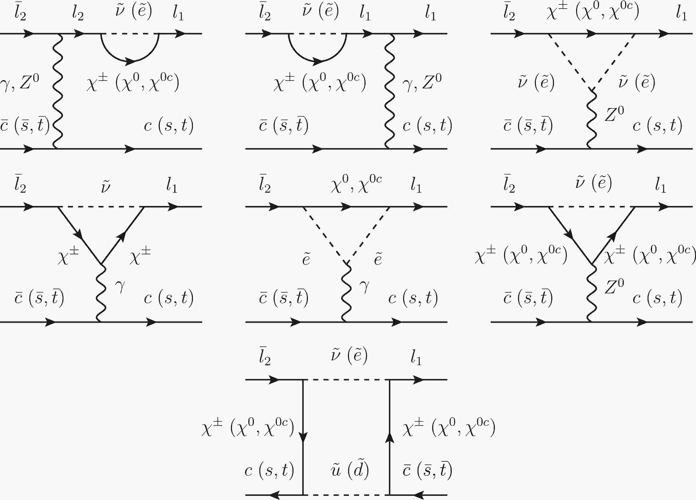
In the following we will discuss the LFV decays
$ V\rightarrow l_1 l_2 $ in detail. The one-loop Feynman diagrams for the LFV decays$ V\rightarrow l_1 l_2 $ in the MRSSM are shown in Fig. 1. The analytical expression of the BR$ (V\rightarrow l_{1} l_{2}) $ is given in terms of the Wilson coefficients using the effective Lagrangian method in which the general effective Lagrangian for$ V\rightarrow l_1 l_2 $ is expressed as [19]
Figure 1. The Feynman diagrams for
$ V\rightarrow l_1 l_2 $ in the MRSSM at the one-loop level.$ \begin{aligned}[b] -\mathcal{L}_{\rm eff} =&m_2(C^{l_1l_2}_{DR}\bar{l}_1\sigma^{\mu\nu}P_Ll_2 +C^{l_1l_2}_{DL}\bar{l}_1\sigma^{\mu\nu}P_Rl_2)F_{\mu\nu}+{\rm h.c}.\\ &+\sum_q\Big[\big(C^{ql_1l_2}_{VR}\bar{l}_1\gamma^{\mu}P_R l_2+C^{ql_1l_2}_{VL}\bar{l}_1\gamma^{\mu}P_L l_2\big)\bar{q}\gamma_{\mu}q\\ &+\big(C^{ql_1l_2}_{AR}\bar{l}_1\gamma^{\mu}P_R l_2+C^{ql_1l_2}_{AL}\bar{l}_1\gamma^{\mu}P_L l_2\big)\bar{q}\gamma_{\mu}\gamma_5 q\\ &+m_2 m_q G_F \big(C^{ql_1l_2}_{SR}\bar{l}_1P_L l_2+C^{ql_1l_2}_{SL}\bar{l}_1P_R l_2\big)\bar{q}q\\ &+m_2 m_q G_F \big(C^{ql_1l_2}_{PR}\bar{l}_1P_L l_2+C^{ql_1l_2}_{PL}\bar{l}_1P_R l_2\big)\bar{q}\gamma_5 q\\ &+m_2 m_q G_F \big(C^{ql_1l_2}_{TR}\bar{l}_1\sigma^{\mu\nu}P_L l_2\\&+C^{ql_1l_2}_{TL}\bar{l}_1\sigma^{\mu\nu}P_R l_2\big)\bar{q}\sigma_{\mu\nu}q+{\rm h.c}.\Big], \end{aligned} $

(10) where the left/right chiral projection operator
$ P_{L/R} = $ $ \dfrac{1}{2}(1\mp\gamma_5) $ ,$ G_F $ stands for the Fermi constant and$ m_q $ stands for the mass of the quark q.$ C^{l_1l_2}_{DL/DR} $ in the first row in Eq. (10) are the dipole Wilson coefficients and thus strongly constrained by the radiative decays of the leptons (i.e.,$ l_1\rightarrow l_2\gamma $ ). The rest are the dimension six four-fermion Lagrangian, where the Wilson coefficients contain the contributions from the Z boson and the Higgs boson excluding the photon.For the LFV decays
$ V\rightarrow l_1 l_2 $ , the general expression of the amplitude is rewritten as [19]$ \begin{aligned}[b] \mathcal{A}(V\rightarrow l_1 l_2) =&\bar{u}(p_1)\Big[A^{l_1l_2}_{V}\gamma^{\mu}+B^{l_1l_2}_{V}\gamma^{\mu}\gamma^{5} +\frac{C^{l_1l_2}_{V}}{m_V}(p_2-p_1)_{\mu} \\&-\frac{ D^{l_1l_2}_{V}}{m_V}(p_2-p_1)_{\mu}\gamma^{5}\Big]\upsilon(p_2)\epsilon^\mu(p), \end{aligned} $

(11) where
$ m_V $ stands for the mass of the vector meson V,$ \epsilon^\mu(p) $ stands for the polarization vector, and p stands for its momentum. The coefficients$ A^{l_1l_2}_{V} $ ,$ B^{l_1l_2}_{V} $ ,$ C^{l_1l_2}_{V} $ , and$ D^{l_1l_2}_{V} $ are dimensionless and can be expressed in terms of the Wilson coefficients in Eq. (10) together with the decay constants. The coefficients in Eq. (11) are derived as [19]$ \begin{aligned}[b] A^{l_1l_2}_{V}=&\sqrt{4\pi\alpha}Q_qy^2(C^{l_1l_2}_{DL}+C^{l_1l_2}_{DR}) +\kappa_V(C^{ql_1l_2}_{VL}+C^{ql_1l_2}_{VR})\\ &+2y^2\kappa_V\frac{f^T_V}{f_V}G_Fm_Vm_q(C^{ql_1l_2}_{TL}+C^{ql_1l_2}_{TR}), \\ B^{l_1l_2}_{V}=&-\sqrt{4\pi\alpha}Q_qy^2(C^{l_1l_2}_{DL}-C^{l_1l_2}_{DR}) -\kappa_V(C^{ql_1l_2}_{VL}-C^{ql_1l_2}_{VR})\\ &-2y^2\kappa_V\frac{f^T_V}{f_V}G_Fm_Vm_q(C^{ql_1l_2}_{TL}-C^{ql_1l_2}_{TR}), \\ C^{l_1l_2}_{V}=&\sqrt{4\pi\alpha}Q_qy(C^{l_1l_2}_{DL}+C^{l_1l_2}_{DR}) \\&+2\kappa_V\frac{f^T_V}{f_V}G_Fm_2m_q(C^{ql_1l_2}_{TL}+C^{ql_1l_2}_{TR}), \end{aligned} $

$ \begin{aligned}[b] D^{l_1l_2}_{V}=&-\sqrt{4\pi\alpha}Q_qy(C^{l_1l_2}_{DL}-C^{l_1l_2}_{DR}) \\&+2\kappa_V\frac{f^T_V}{f_V}G_Fm_2m_q(C^{ql_1l_2}_{TL}-C^{ql_1l_2}_{TR}), \end{aligned} $

(12) where α stands for the fine structure constant,
$ Q_q $ stands for the charge of the quark q, y =$ \dfrac{m_2}{m_V} $ , and$ \kappa_V $ =$ \dfrac{1}{2} $ for the pure$ q\bar{q} $ states. It is noted that, different from the definition of$ D^{l_1l_2}_{V} $ in [19], the imaginary unit was not considered in this work. From Eq. (12) we see that the contributions of the Higgs mediated self-energies and penguin diagrams are nonexistent since these diagrams only contribute to the Wilson coefficients corresponding to the scalar and the pseudo-scalar operators in Eq. (10). The contributions of the tensor operators can be neglected in the MRSSM since the coefficients$ C^{ql_1l_2}_{TL/TR} $ (corresponding to the Feynman diagrams in Fig. 1) are computed as zero. The definitions of the decay constant$ f_V $ and the transverse decay constant$ f^T_V $ are$ \begin{aligned}[b] \left\langle 0\left|\bar{q} \gamma^\mu q\right| V(p)\right\rangle & =f_V m_V \epsilon^\mu(p), \\ \left\langle 0\left|\bar{q} \sigma^{\mu \nu} q\right| V(p)\right\rangle & ={\rm i} f_V^T\left(\epsilon^\mu p^\nu-\epsilon^\nu p^\mu\right) . \end{aligned}$

(13) In the following, we list the general expressions of the Wilson coefficients, where
$ F,~S $ denote the fermion and the scalar particle, respectively. The coefficients$ C^{l_1l_2}_{VL} $ for the self-energy diagrams in Fig. 1 are$ \begin{aligned}[b] C^{ql_1l_2}_{VL}=&\frac{C^{l_2l_2Z}_L}{(m_{l_1}^2-m_{l_2}^2)m_Z^2}(C^{qqZ}_L+C^{qqZ}_R)\\&\times(m_{l_1}^2C^{FSl_1}_LC^{FSl_2*}_RB_1(0,m_{F}^2,m_{S}^2)\\ &-m_{l_1}m_{F}C^{FSl_1}_RC^{FSl_2*}_RB_0(0,m_{F}^2,m_{S}^2)\\&+m_{l_1}m_{l_2}C^{FSl_1}_RC^{FSl_2*}_LB_1(0,m_{F}^2,m_{S}^2)\\ &-m_{l_2}m_{F}C^{FSl_1}_LC^{FSl_2*}_LB_0(0,m_{F}^2,m_{S}^2)), \\ C^{ql_1l_2}_{VL}=&\frac{C^{l_1l_1Z}_L}{(m_{l_1}^2-m_{l_2}^2)m_Z^2}(C^{qqZ}_L+C^{qqZ}_R)\\&\times(m_{l_2}^2C^{FSl_2*}_RC^{FSl_1}_LB_1(0,m_{F}^2,m_{S}^2)\\ &-m_{l_2}m_{F}C^{FSl_2*}_LC^{FSl_1}_LB_0(0,m_{F}^2,m_{S}^2)\\&+m_{l_2}m_{l_1}C^{FSl_2*}_LC^{FSl_1}_RB_1(0,m_{F}^2,m_{S}^2)\\ &-m_{l_1}m_{F}C^{FSl_2*}_RC^{FSl_1}_RB_0(0,m_{F}^2,m_{S}^2)),\end{aligned} $

with
$ FS\in\{\chi^0\tilde{e},\chi^{0c}\tilde{e},\chi^{\pm}\tilde{\nu}\} $ .$ q\in \{c,s,b\} $ depends on the components of the vector mesons.$ C^{qqZ}_{L/R} $ ,$ C^{FSl_1}_{L/R} $ ,..., stand for the interaction of$ q\text{-}q\text{-}Z $ ,$ F\text{-}S\text{-}l_1 $ , etc. The coefficients$ C^{l_1l_2}_{VL} $ for the triangle diagrams in Fig. 1 are$ \begin{aligned}[b] C^{ql_1l_2}_{VL}=&-\frac{2}{m_Z^2}C^{FS_1l_1}_LC^{FS_2l_2*}_RC^{S_1S_2Z}(C^{qqZ}_L+C^{qqZ}_R)\\&\times C^{'}_{00}(m_{F}^2,m_{S_2}^2,m_{S_1}^2),\\ C^{ql_1l_2}_{VL}=&\frac{1}{m_Z^2}C^{F_1Sl_1}_LC^{F_2Sl_2*}_R(C^{F_1F_2Z}_R(B^{'}_0(m_{F_2}^2, m_{F_1}^2, m_S^2)\\&-2C^{'}_{00}(m_{F_2}^2,m_{F_1}^2,m_{S}^2)) \\ &- C^{F_1F_2Z}_LC^{'}_{0}(m_{F_2}^2,m_{F_1}^2,m_{S}^2)m_{F_1}m_{F_2})(C^{qqZ}_L+C^{qqZ}_R), \end{aligned} $

with
$FS_1S_2\in\{\chi^{\pm}\tilde{\nu}\tilde{\nu},~\chi^0\tilde{e}\tilde{e},~\chi^{0c}\tilde{e}\tilde{e}\}$ and$ F_1F_2S\in\{\chi^0\chi^0\tilde{e}, \chi^{0c}\chi^{0c}\tilde{e},\chi^{\pm}\chi^{\pm}\tilde{\nu}\} $ . The coefficients$ C^{l_1l_2}_{DL} $ for the triangle diagrams in Fig. 1 are$ \begin{aligned}[b] C^{ql_1l_2}_{DL}=&\frac{C^{S_1S_2\gamma}}{\sqrt{4\pi\alpha_Z}}(m_{l_1}C^{FS_1l_1*}_RC^{FS_2l_2}_LC^{'}_2(m_F^2, m_{S_2}^2, m_{S_1}^2)\\&+m_{l_2}C^{FS_1l_1*}_LC^{FS_2l_2}_R\\ &\times C^{'}_1(m_F^2, m_{S_2}^2, m_{S_1}^2) - m_{F}C^{FS_1l_1*}_LC^{FS_2l_2}_LC^{'}_0(m_F^2, m_{S_2}^2, m_{S_1}^2 )),\\ C^{ql_1l_2}_{DL}=&\frac{1}{\sqrt{4\pi\alpha_Z}}(m_{l_1}C^{F_1Sl_1*}_RC^{F_2Sl_2}_LC^{F_1F_2\gamma}_LC^{'}_{12}(m_{F_2}^2, m_{F_1}^2, m_{S}^2)\\&-m_{l_2}C^{F_1Sl_1*}_LC^{F_2Sl_2}_R\\ &\times C^{F_1F_2\gamma}_RC^{'}_2(m_{F_2}^2, m_{F_1}^2, m_{S}^2)\\&-m_{F_1}C^{F_1Sl_1*}C^{F_2Sl_2}_LC^{F_1F_2\gamma}_LC^{'}_1(m_{F_2}^2, m_{F_1}^2, m_{S}^2)\\ &+m_{F_2}C^{F_1Sl_1*}C^{F_2Sl_2}_LC^{F_1F_2\gamma}_RC^{'}_0(m_{F_2}^2, m_{F_1}^2, m_{S}^2)), \end{aligned} $

with
$ FS_1S_2\in\{\chi^{\pm}\tilde{\nu}\tilde{\nu},\chi^0\tilde{e}\tilde{e},\chi^{0c}\tilde{e}\tilde{e}\} $ and$F_1F_2S\in\{\chi^0\chi^0\tilde{e},~ \chi^{0c}\chi^{0c}\tilde{e},~\chi^{\pm}\chi^{\pm}\tilde{\nu}\}$ . The coefficients$ C^{l_1l_2}_{VL} $ for the box diagrams in Fig. 1 are$ \begin{aligned}[b] C^{ql_1l_2}_{VL}=&C^{F_1S_1l_1}_LC^{F_2S_1l_2*}_R(\frac{1}{2}C^{F_1S_2q}_RC^{F_2S_2q*}_LD^{'}_0\\&\times(m_{F_1}, m_{F_2}, m_{F_2}^2, m_{F_1}^2, m_{S_1}^2, m_{S_2}^2)\\ &-C^{F_1S_2q}_LC^{F_2S_2q*}_RD^{'}_{00}(m_{F_2}^2, m_{F_1}^2, m_{S_1}^2, m_{S_2}^2)), \end{aligned} $

with
$F_1F_2S_1S_2\in\{\chi^{\pm}\chi^{\pm}\tilde{\nu}\tilde{d}(\tilde{u}),~\chi^0\chi^0\tilde{e}\tilde{u}(\tilde{d}),~\chi^{0c}\chi^0\tilde{e}\tilde{u}(\tilde{d}),~ \chi^0\chi^{0c}\tilde{e}\tilde{u}(\tilde{d}),~ \chi^{0c}\chi^{0c}\tilde{e}\tilde{u}(\tilde{d})\}$ . The coefficients are left-right symmetric, i.e,$ C^{ql_1l_2}_{VR} $ =$ C^{ql_1l_2}_{VL} $ ($ L\leftrightarrow R $ ) and$ C^{ql_1l_2}_{DR} $ =$ C^{ql_1l_2}_{DL} $ ($ L\leftrightarrow R $ ). The explicit expressions of the loop integrals are given elsewhere [57−60]. The expressions of the Wilson coefficients in the MRSSM were added to the Mathematica package SARAH [59−63] to generate modules for the Fortran package SPheno [57, 58].The amplitude in Eq. (11) leads to the branching ratio BR(
$ V\rightarrow l_1 l_2 $ ), which is conveniently given as [19]$ \begin{aligned}[b] {\rm BR}(V\rightarrow l_1 l_2) =&{\rm BR}(V\rightarrow e e)\times \big(\frac{m^2_V(1-y^2)^2}{4\pi\alpha Q_q}\big)^2\\&\times\Big[|A^{l_1l_2}_{V}|^2+|B^{l_1l_2}_{V}|^2\\ &+(\frac{1}{2}-2y^2)\big(|C^{l_1l_2}_{V}|^2+|D^{l_1l_2}_{V}|^2\big) \\&+y {\rm Re}(A^{l_1l_2}_{V}C^{l_1l_2\ast}_{V}+ B^{l_1l_2}_{V}D^{l_1l_2\ast}_{V})\Big], \end{aligned} $

(14) where the mass of the lighter one of the two final leptons is set to zero.
-
In Table 3, we provide a list of values of the vector masses, the decay constants and BR(
$ V\rightarrow ee $ ) used for calculating BR($ V\rightarrow l_1 l_2 $ ); all the mass parameters are in GeV [19, 64]. Following the suggestion in Ref. [65] and the fact that the branching ratio in Eq. (14) is, to a large extent, independent of the value of the decay constant [19], the transverse decay constants of the vectors are the same (i.e.,$ f^T_V $ =$ f_V $ ) except for$ J/\psi $ , which is$ f^T_{J/\psi} $ = 0.410 GeV.Vector ϕ $ J/\psi $ 

$ \psi(2S) $ 

$ \Upsilon(1S) $ 

$ \Upsilon(2S) $ 

$ \Upsilon(3S) $ 

$ m_V $ 

1.0194 3.0969 3.686 9.4603 10.023 10.355 $ f_V $ 

0.241 0.418 0.294 0.649 0.481 0.539 BR( $ V\rightarrow ee $ )

$ 2.973\times 10^{-4} $ 

$ 5.971\times 10^{-2} $ 

$ 7.93\times 10^{-3} $ 

$ 2.38\times 10^{-2} $ 

$ 1.91\times 10^{-2} $ 

$ 2.18\times 10^{-2} $ 

Table 3. Values used in the calculation.
The most accurate prediction for the mass of the SM-like Higgs boson as well as the W boson in the MRSSM was given in Ref. [43], with the following set of benchmark points:
$ \begin{aligned}[b]& \mu_{u}=\mu_{d}=500,M_D^W=600,M_D^B=550,\Lambda_d=-1.2,\lambda_d=1.0,\\& \Lambda_u=-1.1,\lambda_u=-0.8,B_\mu=500^2,v_S=5.9,{\rm tan}\beta=3,\\& (m^2_l)_{ii}=(m^2_r)_{ii}=1000^2\;(i=1,2,3),v_T=-0.38, \end{aligned} $

$ \begin{aligned}[b]& (m^2_{\tilde{q}})_{ii}=(m^2_{\tilde{u}})_{ii}=(m^2_{\tilde{d}})_{ii}=2500^2\;(i=1,2),m_T=3000,\\& (m^2_{\tilde{q}})_{ii}=(m^2_{\tilde{u}})_{ii}=(m^2_{\tilde{d}})_{ii}=1000^2\;(i=3),m_S=2000, \end{aligned} $

(15) where the mass parameters are in GeV or GeV
$ ^2 $ . The predicted W boson mass in the MRSSM is comparable with the result from the combined Large Electron-Positron (LEP) collider and Fermilab Tevatron collider measurements [66], the result from the ATLAS collaboration [67] and the result from the LHCb Collaboration [68], which is more precise than the LEP result. By changing the values of some parameters, e.g.$m_{\rm SUSY}$ ,$ v_T $ ,$ \Lambda_u $ and$ \Lambda_d $ , the recent result for the W boson mass obtained by the CDF collaboration [69] can also be accommodated in the MRSSM [43, 53]. It is noted that these parameters have very little effect on the predicted BR($ V\rightarrow l_1 l_2 $ ), which takes values within a narrow range. The default values of the input parameters are given in Eq. (15) in the following analysis. Note that the off-diagonal inputs of the slepton mass matrices$ m^2_l $ ,$ m^2_r $ as well as the squark mass matrices$ m^2_{\tilde{q}} $ ,$ m^2_{\tilde{u}} $ ,$ m^2_{\tilde{d}} $ in Eq. (15) are zero.The LFV decays arise from the off-diagonal inputs of the
$ 3\times3 $ slepton mass matrices$ m_{l}^{2} $ and$ m_{r}^{2} $ . These off-diagonal inputs of matrices$ m_{l}^{2} $ and$ m_{r}^{2} $ are usually parameterized by the mass insertions$ \begin{aligned}[b]& (m^{2}_l)^{IJ}=\delta ^{IJ}_l\sqrt{(m^{2}_l)^{II}(m^{2}_l)^{JJ}},\; \\& (m^{2}_r)^{IJ}=\delta ^{IJ}_r\sqrt{(m^{2}_r)^{II}(m^{2}_r)^{JJ}},(I,J=1,2,3).\nonumber \end{aligned} $

Before the numerical computation, some assumptions were made to decrease the number of free parameters. The parameters
$ \delta^{IJ}_l $ and$ \delta^{IJ}_r $ were strongly constrained by the experimental limitations on several LFV decays, for example, the radiative two body decays ($ l_2\rightarrow l_1\gamma $ ), the leptonic three body decays ($ l_2\rightarrow 3l_1 $ ), and$ \mu-e $ conversions in nuclei. We list the current limits of the above LFV decays in Table 4 [64]. Both$ \delta^{IJ}_l $ and$ \delta^{IJ}_r $ have a perceptible effect on the prediction of the branching ratio of the lepton flavor violating processes, with$ \delta^{IJ}_l $ having a stronger effect than$ \delta^{IJ}_r $ . For simplicity and for obtaining larger predictions of the branching ratios, we assumed$ \delta ^{IJ}_{l} $ =$ \delta ^{IJ}_{r} $ =$ \delta ^{IJ} $ and then$ \delta ^{IJ} $ =$ \delta ^{12} $ ,$ \delta ^{13} $ or$ \delta ^{23} $ . In the following we used the experimental limits in Table 4 to constrain the parameters$ \delta^{IJ} $ .Decay Limit Decay Limit Decay Limit Decay Limit $ \mu\rightarrow e\gamma $ 

$ 4.2\times 10^{-13} $ 

$ \mu\rightarrow 3e $ 

$ 1.0\times 10^{-12} $ 

$ \tau\rightarrow e\gamma $ 

$ 3.3\times 10^{-8} $ 

$ \tau\rightarrow 3e $ 

$ 2.7\times 10^{-8} $ 

$ \tau\rightarrow \mu\gamma $ 

$ 4.4\times 10^{-8} $ 

$ \tau\rightarrow 3\mu $ 

$ 2.1\times 10^{-8} $ 

$ \mu-e $ ,Ti

$ 4.3\times 10^{-12} $ 

Table 4. Current limits on the
$ l_1\rightarrow l_2\gamma $ ,$ l_1\rightarrow 3 l_2 $ and$ \mu-e $ conversions for Ti targets.We give the corresponding predictions for BR(
$ V\rightarrow l_1 l_2 $ ) in Fig. 2 along with the other SUSY parameters in Eq. (15) where the predictions for BR($ l_1\rightarrow l_2\gamma $ ), BR($ l_1\rightarrow 3 l_2 $ ) and CR($ \mu-e $ , Ti) are also presented. Results are shown as functions of one of the parameters$ \delta^{IJ} $ . In all plots, only the indicated$ \delta^{IJ} $ is varied with all other mass insertions set to zero. The predictions for BR($ \Upsilon(nS)\rightarrow l_1l_2 $ ) in each plot are very close to each other. The predictions for BR($ V\rightarrow e^{-}\mu^{+} $ ), BR($ V\rightarrow e^{-}\tau^{+} $ ), and BR($ V\rightarrow \mu^{-} \tau^{+} $ ) were affected by the mass insertions$ \delta^{12} $ ,$ \delta^{13} $ , and$ \delta^{23} $ , respectively. The predicted BR($ V\rightarrow l_1l_2 $ ) in the MRSSM was below$ 10^{-14} $ and was at least seven orders of magnitude below the current experimental limit. A linear relationship was obtained between the branching ratios and the flavor violating parameters$ \delta^{IJ} $ owing to the fact that both x axis and y axis in Fig. 2 were logarithmically scaled. The actual dependence on$ \delta^{IJ} $ was quadratic. The following hierarchy is shown in Fig. 2, BR($ \Upsilon(3S)\rightarrow l_1 l_2 $ )$ > $ BR($ \Upsilon(2S)\rightarrow l_1 l_2 $ )$ \sim $ BR($\Upsilon(1S) \rightarrow l_1l_2$ )$ > $ BR($ J/\psi\rightarrow l_1 l_2 $ )$ > $ BR($\psi(2S) \rightarrow l_1 l_2$ )$ > $ BR($\phi \rightarrow l_1 l_2$ ). The same hierarchy appeared in several new physics scenarios [1, 14]. The most challenging experimental prospects for$ \delta^{12} $ arose for$ \mu\rightarrow e\gamma $ . Considering that the new sensitivity for BR($ \mu\rightarrow e\gamma $ ) will be approximately$ 6\times 10^{-14} $ in the future projects of MEG II [70],$ \delta^{12} $ was constrained to be approximately$ 10^{-3} $ . The constraints on$ \delta^{13} $ from$ \tau\rightarrow e\gamma $ and$ \tau\rightarrow 3e $ were comparable, and$ \delta^{13} $ was constrained to be approximately$ 10^{-0.2} $ . The case for$ \delta^{23} $ was the same as that for$ \delta^{13} $ .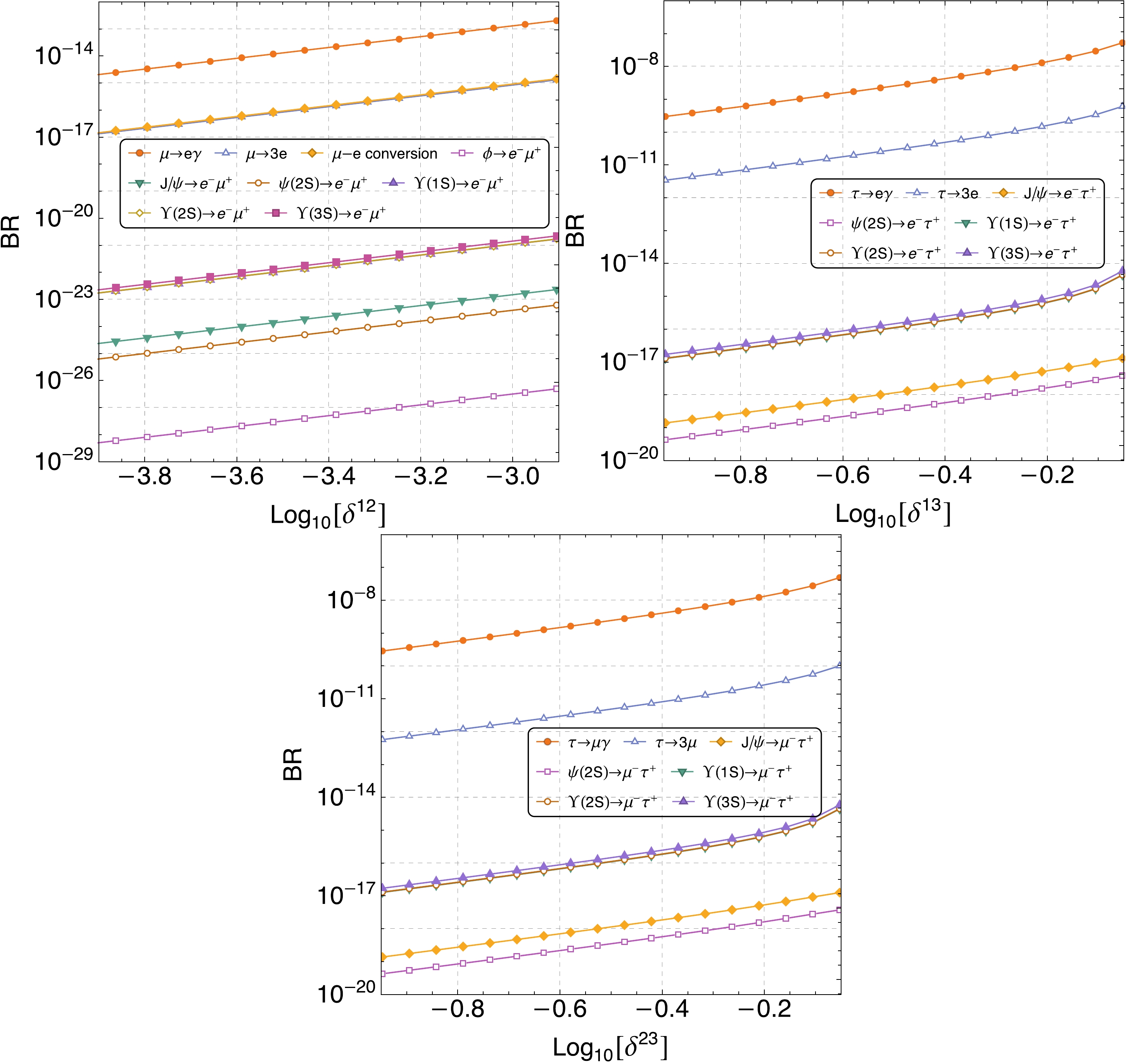
Figure 2. (color online) Predictions for BR(
$ V\rightarrow l_1 l_2 $ ) in the MRSSM. Note that the predictions for BR($ \Upsilon(nS)\rightarrow l_1 l_2 $ ) in each plot are very close to each other.In the following, we consider the process
$ \Upsilon(3S)\rightarrow l_1l_2 $ as an example since the behavior for$ \Upsilon(3S) $ also exists for ϕ,$ J/\psi $ ,$ \psi(2S) $ ,$ \Upsilon(1S) $ , and$ \Upsilon(2S) $ . We present the corresponding predictions for BR($ \Upsilon(3S)\rightarrow l_1 l_2 $ ) from various parts as functions of tanβ in Fig. 3, where$ \delta^{12} $ =$ 10^{-3} $ ($ e\mu $ ),$ \delta^{13} $ =$ 10^{-0.2} $ ($ e\tau $ ), and$ \delta^{23} $ =$ 10^{-0.2} $ ($ \mu\tau $ ) are used. The lines corresponding to "Z," "γ," and "Box" stand for the values of BR($ \Upsilon(3S)\rightarrow l_1 l_2 $ ) obtained by only considering the listed contribution without any others. The predicted BR($ \Upsilon(3S)\rightarrow l_1 l_2 $ ) with the total contribution is also indicated. We observe that the contributions from different parts are comparable, and the following order holds: BR($ \Upsilon(3S)\rightarrow l_1 l_2 $ , Z)$ > $ BR($ \Upsilon(3S)\rightarrow l_1 l_2 $ , Total)$ > $ BR ($ \Upsilon(3S)\rightarrow l_1 l_2 $ , γ)$ > $ BR ($J/\psi\rightarrow l_1 l_2$ , Box) (for$ J/\psi $ ,$ \psi(2S) $ , BR($ \Upsilon(3S)\rightarrow l_1 l_2 $ , γ)$ > $ BR($ \Upsilon(3S)\rightarrow l_1 l_2 $ , Total)). For small values of$ \tan \beta $ , the prediction for Z penguin changes quickly, since the branching ratios are proportional to the reciprocal of$ \tan \beta^2 $ , and for the same reason, the prediction for Z penguin changes slowly for higher values of$ \tan \beta $ . This behavior is also observed for the$ \mu-e $ conversion [38, 71] and for the$ \tau\rightarrow Pl $ process [55], both of which gain the contribution from the similar Z penguin diagrams excluding the quark sector.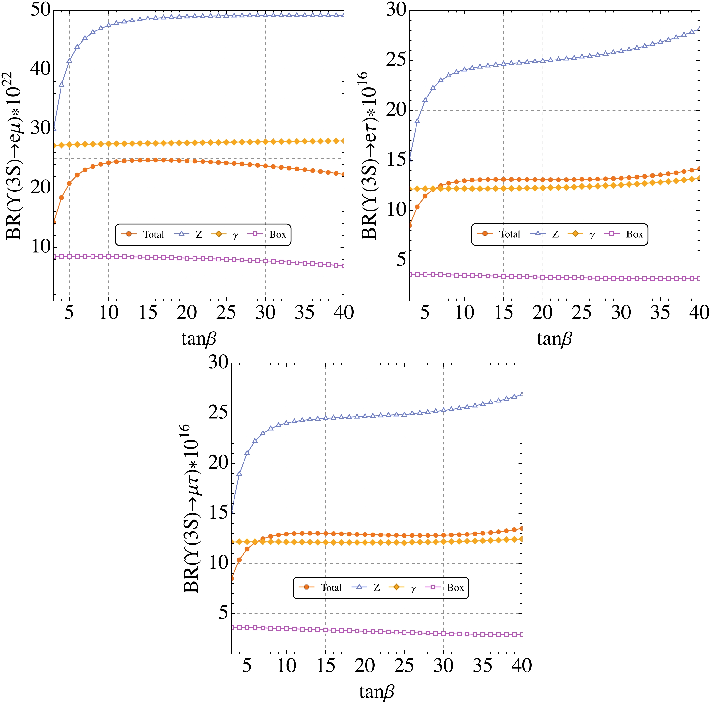
Figure 3. (color online) Contributions to BR(
$ \Upsilon(3S)\rightarrow l_1 l_2 $ ) from various parts in the MRSSM.We present the contour plots of BR(
$ \Upsilon(3S)\rightarrow l_1 l_2 $ ) in the mQ$ \sim $ mL plane in Fig. 4, where mQ=$ \sqrt{(m^2_{\tilde{q}})_{ii}}= \sqrt{(m^2_{\tilde{u}})_{ii}}=\sqrt{(m^2_{\tilde{d}})_{ii}} $ ($ i=1, 2, 3 $ ) and mL=$ \sqrt{(m^2_l)_{ii}}=\sqrt{(m^2_r)_{ii}} $ ($ i=1, 2, 3 $ ) are assumed. The predictions for BR($ \Upsilon(3S)\rightarrow l_1l_2 $ ) are sensitive to mQ and mL. The predictions for BR($ \Upsilon(3S)\rightarrow l_1l_2 $ ) increase slowly when the parameter mQ varies from 1 TeV to 5 TeV and decrease slowly when the parameter mL varies from 1 TeV to 5 TeV. For a wide range of mQ and mL values, the predictions for BR($ \Upsilon(3S)\rightarrow l_1 l_2 $ ) change by approximately one order of magnitude. The off-diagonal inputs$ \delta^{IJ}_{\tilde{q},\tilde{u},\tilde{d}} $ of the mass matrices$ m^2_{\tilde{q}} $ ,$ m^2_{\tilde{u}} $ and$ m^2_{\tilde{d}} $ have very little effect on the predicted BR($ \Upsilon(3S)\rightarrow l_1 l_2 $ ), which takes values in a narrow range. The effect from the off-diagonal inputs of the squark mass matrics is too small to be neglected. It is noted that the effects of the other parameters in Eq. (15) are the same as those described in Refs. [55, 56].
Figure 4. (color online) Contour plots showing the behavior of BR(
$ \Upsilon(3S)\rightarrow l_1 l_2 $ ) as a function of mQ and mL.The final results on the upper bounds of BR(
$ V\rightarrow l_1l_2 $ ) in the MRSSM are given in Table 5; those were obtained by assuming$ \delta^{12} $ =$ 10^{-3} $ ,$ \delta^{13} $ =$ 10^{-0.2} $ ($ \approx 0.63 $ ) and$ \delta^{23} $ =$ 10^{-0.2} $ , respectively, and the results in the literature are also included for comparison. Using an effective field theory, the data in Ref. [20] were obtained from the recast of high-$ p_T $ dilepton tails at the LHC for the left-handed scenario, where dipole operators were not considered. The expressions for BR($ V\rightarrow l_1 l_2 $ ) in Ref. [20] were the same, except for a few adjustments (e.g., mass, decay constant and full width). Since the mass, decay constant and full width for$ \psi(2S) $ are very close to$ J/\psi $ , the bounds for$ \psi(2S)\rightarrow l_1l_2 $ were on the same level as$ J/\psi\rightarrow l_1 l_2 $ . For the same reason, the bounds for$ \Upsilon(1S)\rightarrow l_1 l_2 $ and$ \Upsilon(2S)\rightarrow l_1 l_2 $ were on the same level as$ \Upsilon(3S)\rightarrow l_1 l_2 $ . The predicted values for BR($ V\rightarrow l \tau $ ) in the MRSSM ranged between the values reported in Ref. [1] and Ref. [14], and the predicted values for BR($ V\rightarrow e \mu $ ) were below those reported in Ref. [1] and Ref. [14]. All the direct bounds in new physics scenarios were smaller than the indirect bounds in Ref. [20]. The limits on BR($ V\rightarrow l_1 l_2 $ ) in the MRSSM were more than ten orders of magnitude smaller than the current limits or future experimental sensitivities [24, 27, 29, 72].Decay Ref. [20](3 ab $ ^{-1} $ )

Ref. [1]((2,3)-ISS) Ref. [14](331) this work (MRSSM) $ \phi\rightarrow e\mu $ 

$ 1.2\times 10^{-18} $ 

$ 1\times 10^{-23} $ 

$ 8.1\times 10^{-23} $ 

$ 3.2\times 10^{-27} $ 

$ J/\psi\rightarrow e\mu $ 

$ 1.6\times 10^{-12} $ 

$ 2\times 10^{-20} $ 

$ 7.7\times 10^{-20} $ 

$ 1.5\times 10^{-23} $ 

$ J/\psi\rightarrow e\tau $ 

$ 4.8\times 10^{-12} $ 

$ 1\times 10^{-19} $ 

$ 6.3\times 10^{-15} $ 

$ 5.3\times 10^{-18} $ 

$ J/\psi\rightarrow \mu\tau $ 

$ 6.4\times 10^{-12} $ 

$ 4\times 10^{-19} $ 

$ 5.2\times 10^{-15} $ 

$ 5.3\times 10^{-18} $ 

$ \psi(2S)\rightarrow e\mu $ 

- $ 4\times 10^{-21} $ 

$ 2.1\times 10^{-20} $ 

$ 3.9\times 10^{-24} $ 

$ \psi(2S)\rightarrow e\tau $ 

- $ 4\times 10^{-20} $ 

$ 2.1\times 10^{-15} $ 

$ 1.6\times 10^{-18} $ 

$ \psi(2S)\rightarrow \mu\tau $ 

- $ 1\times 10^{-19} $ 

$ 1.7\times 10^{-15} $ 

$ 1.6\times 10^{-18} $ 

$ \Upsilon(1S)\rightarrow e\mu $ 

- $ 2\times 10^{-19} $ 

$ 3.8\times 10^{-17} $ 

$ 1.0\times 10^{-21} $ 

$ \Upsilon(1S)\rightarrow e\tau $ 

- $ 6\times 10^{-18} $ 

$ 5.5\times 10^{-12} $ 

$ 6.4\times 10^{-16} $ 

$ \Upsilon(1S)\rightarrow \mu\tau $ 

- $ 1\times 10^{-17} $ 

$ 4.3\times 10^{-12} $ 

$ 6.4\times 10^{-16} $ 

$ \Upsilon(2S)\rightarrow e\mu $ 

- $ 2\times 10^{-19} $ 

$ 4.2\times 10^{-17} $ 

$ 1.1\times 10^{-21} $ 

$ \Upsilon(2S)\rightarrow e\tau $ 

- $ 8\times 10^{-18} $ 

$ 6.1\times 10^{-12} $ 

$ 6.5\times 10^{-16} $ 

$ \Upsilon(2S)\rightarrow \mu\tau $ 

- $ 2\times 10^{-17} $ 

$ 4.8\times 10^{-12} $ 

$ 6.5\times 10^{-16} $ 

$ \Upsilon(3S)\rightarrow e\mu $ 

$ 1.3\times 10^{-9} $ 

$ 5\times 10^{-19} $ 

$ 9.1\times 10^{-17} $ 

$ 1.4\times 10^{-21} $ 

$ \Upsilon(3S)\rightarrow e\tau $ 

$ 7.9\times 10^{-9} $ 

$ 2\times 10^{-17} $ 

$ 1.3\times 10^{-11} $ 

$ 8.5\times 10^{-16} $ 

$ \Upsilon(3S)\rightarrow \mu\tau $ 

$ 1.2\times 10^{-8} $ 

$ 3\times 10^{-17} $ 

$ 1.0\times 10^{-11} $ 

$ 8.5\times 10^{-16} $ 

Table 5. The upper limits on BR(
$ V\rightarrow l_1 l_2 $ ) in literature and in the MRSSM. -
Although higher order LFV processes in the SM are permitted, these are extremely suppressed by the powers of small neutrino masses, making it impossible to obtain LFV signals in current and future experiments. From this point of view, observations of the LFV decays could indicate new physics, beyond the SM.
In this study, we analyzed the LFV decays of vector mesons
$ V\rightarrow l_1 l_2 $ in the framework of the MRSSM, accounting for the constraints on the mass insertion parameters$ \delta^{ij} $ from the radiative charged lepton decays ($ l_1\rightarrow l_2\gamma $ ), leptonic three body decays ($ l_1\rightarrow 3l_2 $ ), and$ \mu-e $ conversion in nuclei. The predictions for BR($ V\rightarrow e^-\mu^+ $ ), BR($ V\rightarrow e^-\tau^+ $ ), and BR($ V\rightarrow \mu^- \tau^+ $ ) were dominated by the mass insertions$ \delta^{12} $ ,$ \delta^{13} $ , and$ \delta^{23} $ , respectively. It is thought that the LFV decays of mesons may be significantly enhanced by the off-diagonal inputs$ \delta^{IJ}_{\tilde{q},\tilde{u},\tilde{d}} $ . However, as far as we know, this depends on the structure of mesons. The enhancement would be large for the mesons containing two different generation quarks and small for those containing two same generation quarks. For the vector mesons$ J/\psi $ ,$ \Upsilon(nS) $ , and ϕ, the effect from the off-diagonal inputs of the squark mass matrics would be too small to be neglected. The final results for the upper bounds of BR($ V\rightarrow l_1l_2 $ ) in the MRSSM are given in Table 5 and were obtained by assuming$ \delta^{12} = $ $ 10^{-3} $ ,$ \delta^{13} $ =$ 10^{-0.2} $ , and$ \delta^{23} $ =$ 10^{-0.2} $ , respectively. Literature results were also included for comparison. The predictions for BR($ V\rightarrow l_1 l_2 $ ) in the MRSSM were much smaller than the current upper limits.The studies of the radiative LFV (RLFV) decays of vector mesons
$ V\rightarrow \gamma l_1 l_2 $ showed that the RLFV decays might be a new way to search for new physics [19]. Besides the dipole, vector, and tensor operators, the RLFV decays$ V\rightarrow \gamma l_1 l_2 $ could receive contributions through the axial, scalar, and pseudoscalar operators, which are not accessible in the Feynman diagrams of$ V\rightarrow l_1 l_2 $ , e.g., the Higgs mediated self-energies and penguin diagrams. If only considering the contribution from the scalar operators [22], the indirect upper limits on BR$ (\Upsilon(1S)\rightarrow \gamma l_1 \tau) $ could be approximately two to three orders of magnitude smaller than the current result from the Belle collaboration [27]. It might be possible that the RLFV processes$ V\rightarrow \gamma l_1 l_2 $ could be enhanced close to the sensitivities of the current or planned experiment, while the LFV decays$ V\rightarrow l_1 l_2 $ remain out of the reach of current experiments.
Lepton flavor violating decays of vector mesons in the MRSSM
- Received Date: 2023-02-03
- Available Online: 2023-07-15
Abstract: In this study, we analyze the rare decays of the neutral vector mesons


 DownLoad: