


 Abstract
 HTML
HTML Reference
 Related
 PDF
PDF


-
The current resolution of experimental and observational data on gravitational interactions in strong and weak field regimes is consistent with general relativity. However, to the best of our knowledge, general relativity cannot be unified with quantum field theory. An attempt to create a quantum gravity theory was proposed by Hořava, referred to as Hořava-Lifshitz (HL) theory [1−8]. HL theory was especially inspired by Lifshitz theory in solid-state physics. This theory enables us to acquire different solutions and black hole (BH) thermodynamics. In the high energy limit, this theory breaks the Lorentz invariance, and in the low energy limit, it reduces to standard general relativity. Thus, the extended version of general relativity can be considered as one of the candidates for the unified theory of interactions.
The action of HL theory has a complex form, and it is difficult to obtain a general field equation. However, one may derive a so-called effective equation for the gravitational field [9−11]. A spherical-symmetric solution of the effective field theory of HL theory in the infrared (IR) regime was found by Kehagias and Sfetsos [12]. This solution, usually referred to as the KS solution, was later analyzed in Refs. [13, 14]. One of the interesting aspects of this solution is that depending on the value of the coupling parameter of the solution, it may describe both BHs and naked singularities and asymptotically represents the Schwarzschild characteristics. In Ref. [15], the possibility of observationally verifying Hořava gravity on a Solar System scale was explored by considering the classical tests of general relativity for the Kehagias-Sfetsos (KS) asymptotically flat BH solution of HL gravity. The authors of Ref. [16] explored equations of motion and later obtained spherically symmetric solutions for the ultra-violet (UV) regime of HL gravity. A noteworthy characteristic of a KS BH is its violation of the cosmic censorship hypothesis, which postulates that any singularity that emerges in the cosmos should be concealed by an event horizon. In a KS BH, the singularity is naked because it is not obscured by an event horizon and can be observed by distant observers. This violation of cosmic censorship is caused by the modified structure of spacetime in the HL theory of gravity, which permits the formation of naked singularities under certain conditions. The circular motion of particles around a KS naked singularity was analyzed in [17]. Using the slow rotation approximation, the solution for a BH in the IR regime was found in Refs. [18, 19]. The properties of the accretion disk around a BH as well as particle dynamics were analyzed in [20−25]. The shadow of a rotating BH in HL gravity was discussed in [26]. KS BHs have been the subject of many studies and debates in the physics community because they provide a testing ground for the HL theory of gravity and challenge our understanding of the nature of singularities and the cosmic censorship hypothesis. Therefore, in this study, we probe HL gravity using particle dynamics, the plasma effect on shadows, and weak gravitational lensing.
Any new theory should undergo experimental and observational tests for consistency. Optical properties, especially light propagation in a curved background, can be considered useful tools to test the metric theories of gravity. Moreover, the observation of a shadow by the EHT collaboration has forced researchers to test the modified theories of gravity using the optical properties of spacetime [27−30]. Light propagation in the curved spacetime is affected by curvature and, consequently, strong gravity. Owing to captured photons by the central BH, an observer may detect a black spot on the celestial plane. This black spot may be referred to as a BH shadow, and the concept of this phenomenon was first proposed by Synge [31] and later developed by Luminet [32] and Bardeen [33]. The BH shadow has since been extensively studied by various authors [34−57].
The effect of gravitational lensing from light deflection due to spacetime curvature has also been extensively studied by various authors [58−65]). Light propagation is sensitive to the plasma surrounding compact gravitating objects (for example reviews, see [66−74]). The effects of different configurations of plasma on light propagation have been studied in [75−95].
In this paper, we explore light propagation around a BH in HL gravity. The paper is organized as follows: Sec. II is devoted to reviewing the particle dynamics around a BH with the KS parameter. Next, we study the shadow of the BH in HL gravity in Sec. III. Weak gravitational lensing around the BH is analyzed in Sec. IV, and the observable quantities of light deflection are discussed in Sec. V for uniform and non-uniform plasma cases. We summarize the obtained results in Sec. VI. Throughout the paper, we use the geometrical system of units, where
$ G = 1 = c $ . Moreover, Latin (Greek) indices run from 1(0) to 3. -
The spacetime metric in HL gravity with the KS parameter can be written as [12]
$ {\rm d}s^2 = - f(r) {\rm d}t^2 + \frac{{\rm d}r^2}{f(r)} + r^2 ({\rm d} \theta^2 + \sin^2 \theta {\rm d} \phi^2 ) \ , $

(1) where
$ f(r) \equiv 1 + r^2\Omega\left(1-\sqrt{1+4M/(\Omega r^3)}\right) \ , $

(2) and Ω is the KS parameter in HL theory. In the limiting case, when
$ \Omega\to\infty $ , it coincides with Schwarzschild geometry.Now, we study the horizon structure of a BH in HL gravity using the general condition
$ f(r) = 0 $ and easily obtain the event horizon of the BH with the KS parameter,$ r_h = M \pm \sqrt{M^2-\dfrac{1}{2 \Omega }} $ .Next, we consider the motion of a test particle around a BH in HL gravity. To find the trajectory of the test particle, we must consider the Lagrangian of the test particle with mass m in the following form:
$ L' = \frac{1}{2}g_{\mu \nu}u^{\mu}u^{\nu}\ , u^{\mu} = \frac{{\rm d}x^{\mu}}{{\rm d}\tau}, $

(3) where τ is an affine parameter, and
$ x^{\mu} $ and$ u^{\mu} $ are the coordinates and four-velocity of the test particle, respectively. The conserved quantities of the particle motion, such as the energy$ {\cal{E}} $ and angular momentum$ {\cal{L}} $ of the test particle can be written in the following form$ \begin{aligned}[b] {\cal{E}} = & \frac{\partial L'}{\partial u^t} = -f(r)\frac{{\rm d}t}{{\rm d}\tau}\ , \\ {\cal{L}} = & \frac{\partial L'}{\partial u^{\phi}} = r^2\sin^2\theta \frac{{\rm d}\phi}{{\rm d}\tau}\ . \end{aligned} $

(4) By inserting the expressions in (4) into the normalization condition
$ g_{\mu \nu}u^{\mu}u^{\nu} = -\epsilon $ , we can easily obtain the equations of motion of the test particle:$ \frac{{\rm d}r}{{\rm d}\tau} = \sqrt{{\cal{E}}^2-f(r)\left(\epsilon+\frac{{\cal{K}}}{r^2}\right)}, $

(5) $ \frac{{\rm d}\theta}{{\rm d}\tau} = \frac{1}{r^2}\sqrt{{\cal{K}}-\frac{{\cal{L}}^2}{\sin^2\theta}}, $

(6) $ \frac{{\rm d}\phi}{{\rm d}\tau} = \frac{{\cal{L}}^2}{r^2\sin^2\theta}, $

(7) $ \frac{{\rm d}t}{{\rm d}\tau} = \frac{{\cal{E}}}{f(r)}, $

(8) where
$ {\cal{K}} $ is the Carter constant, and the parameter ϵ is defined as$ \epsilon = \left\{ {\begin{array}{*{20}{l}} {1,\ \ \ \ \ {\rm{for}}\;\;{\rm{timelike}}\;\;{\rm{geodesics,}}}\\ {0,\ \ \ \ \ {\rm{for}}\;\;{\rm{null}}\;\;{\rm{geodesics,}}}\\ { - 1,\ \ \ \ \ {\rm{for}}\;\;{\rm{spacelike}}\;\;{\rm{geodesics}}.} \end{array}} \right.$

(9) For simplicity, we can explore the motion of the particle in the equatorial plane, where
$ \theta = \dfrac{\pi}{2} $ and$\dfrac{{\rm d}\theta}{{\rm d}\tau} = 0$ . In this special case, the Carter constant takes the form$ {\cal K} = {\cal L}^2 $ , and the equation for radial motion takes the form$ \left(\frac{{\rm d}r}{{\rm d}\tau}\right)^2 = {\cal E}^2-V_{\rm eff}(r) = {\cal E}^2-f(r)\left(1+\frac{{\cal L}^2}{r^2}\right), $

(10) where
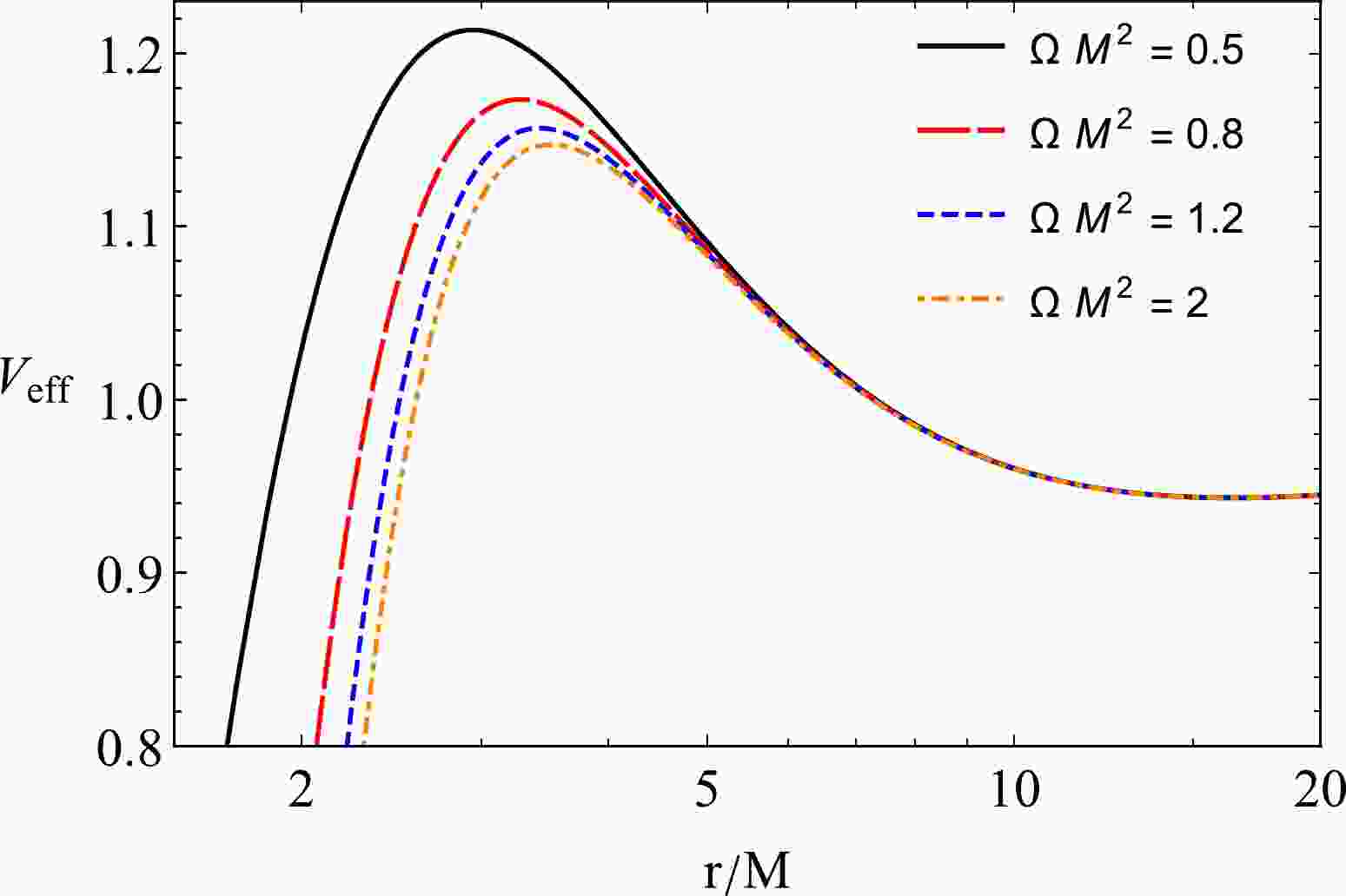
$ V_{\rm eff} = f(r)\left(1+\frac{ {\cal{L}}^2}{r^2}\right), $

(11) is the effective potential of the radial motion of the test particle. The radial dependence of the effective potential of a massive test particle around the BH in HL gravity for different values of the KS parameter Ω is presented in Fig. 1.
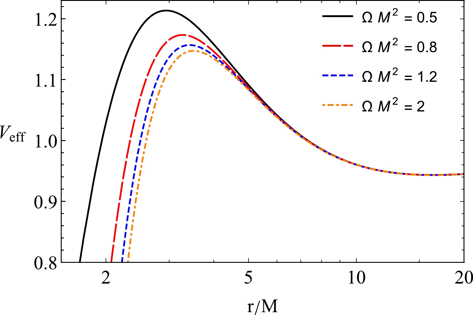
Figure 1. (color online) Radial dependence of effective potential
$V_{\rm eff}$ of a massive particle for different values of the BH parameter$\Omega M^2 $ .To derive the circular motion of the neutral particle around the BH, we can use the conditions
$ \dot{r} = 0 $ and$ \ddot{r} = 0 $ . These conditions allow us to obtain expressions for the energy$ \cal E $ and angular momentum$ \cal L $ of the test particle in the following form:$ {\cal{L}}^2 = \frac{r^5 \Omega \left(\sqrt{\dfrac{4 M}{r^3 \Omega}+1}-1\right)-M r^2}{r \sqrt{\dfrac{4 M}{r^3 \Omega}+1}-3 M}, $

(12) $ \begin{aligned}[b] {\cal{E}}^2 =&\left(\frac{M-r^3 \Omega \left(\sqrt{\dfrac{4 M}{r^3 \Omega}+1}-1\right)}{3 M-r \sqrt{\dfrac{4 M}{r^3 \Omega}+1}}+1\right) \\&\times\left(r^2 \Omega \left(1 - \sqrt{\frac{4 M}{r^3 \Omega}+1}\right)+1\right) \end{aligned} $

(13) Figure 2 shows the radial profiles of the energy
$ \cal E $ and angular momentum$ \cal L $ of the test particle along circular stable orbits around an object in HL spacetime.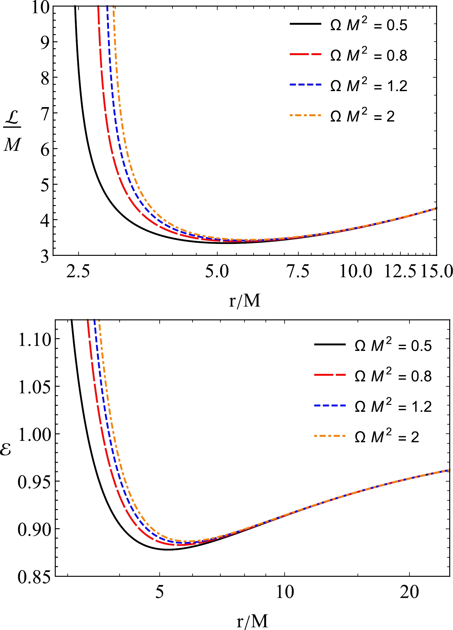
Figure 2. (color online) Radial dependence of
${\cal{L}}$ and${\cal E}$ for different values of the$\Omega M^2 $ parameter.We study the radius of the innermost stable circular orbit (ISCO), hereafter referred to as
$ r_{\rm ISCO} $ . To consider the ISCO radius, we must apply the following general conditions:$ \left\{ {\begin{array}{*{20}{l}} {{{V'}_{\rm eff}} = 0}\\ {{{V''}_{\rm eff}} = 0.} \end{array}} \right. $

(14) From the above conditions, we cannot obtain an analytical expression for the radius
$r_{\rm ISCO}$ . However, we can numerically present the radius of the ISCO using a plot of various values of the parameter Ω, as shown in Fig. 3. From this figure, we can obtain information about the dependence of the ISCO radius on the parameter Ω in HL gravity. The ISCO radius decreases under the influence of the parameter Ω.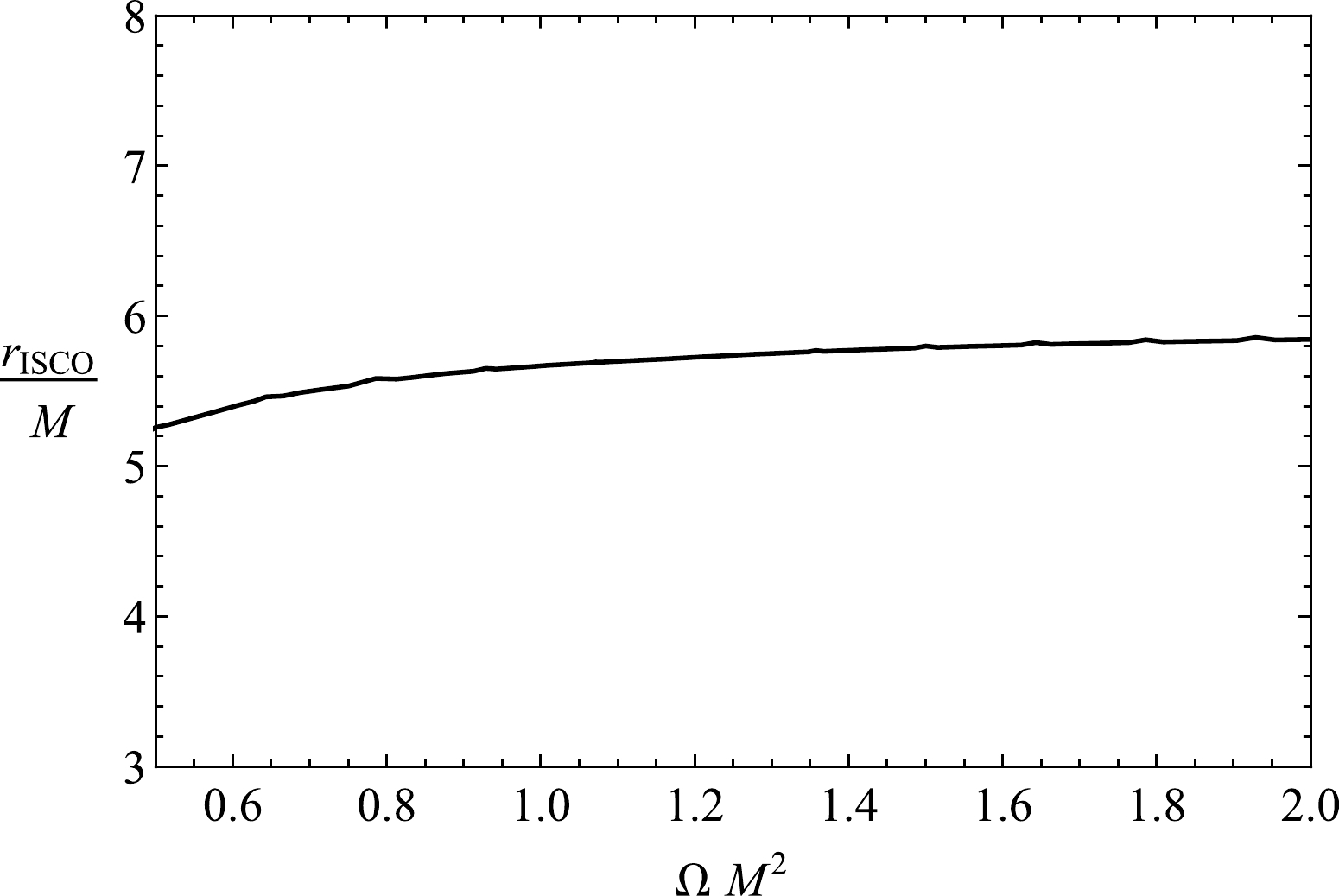
Figure 3. Dependence of the ISCO radius on the
$\Omega M^2 $ parameter. -
Now, we investigate the massless particle motion around a BH in the HL spacetime metric by varying the BH parameters.
-
Here, to study photon motion, we can apply the Hamilton-Jacobi equation and the Hamiltonian of a photon orbiting a BH surrounded by plasma, expressed as [96]
$ {\cal{H}}(x^\alpha, p_\alpha) = \frac{1}{2}\left[ g^{\alpha \beta} p_\alpha p_\beta - (n^2-1)( p_\beta u^\beta )^2 \right]\ , $

(15) where
$ x^\alpha $ are the spacetime coordinates,$ p_\alpha $ and$ u^\beta $ are the four-momentum and four-velocity of the photon, respectively, and n is the refractive index ($ n = \omega/k $ , where k is the wave number). In the case of plasma contribution, the refractive index is expressed as [97]$ n^2 = 1- \frac{\omega_{{p}}^2}{\omega^2}\ , $

(16) and in terms of the plasma frequency
$\omega^2_{p}(x^\alpha) = 4 \pi {\rm e}^2 N(x^\alpha)/m_e$ (where e and$ m_e $ are the electron charge and mass, respectively, and N is the number density of electrons), the photon frequency$ \omega(x^\alpha) $ is defined by$ \omega^2 = ( p_\beta u^\beta )^2 $ $ \omega(r) = \frac{\omega_0}{\sqrt{f(r)}}\ ,\qquad \omega_0 = \text{const}\ . $

(17) The lapse function is such that
$ f(r) \to 1 $ as$ r \to \infty $ and$ \omega(\infty) = \omega_0 = -p_t, $ which shows the energy of the photon at spatial infinity [66]. Moreover, the plasma frequency can be sufficiently smaller than the photon frequency$(\omega_{{p}}^2\ll \omega^2)$ , which allows the BH shadow to be differentiated from the vacuum case ($\omega_{{p}} = 0$ ). The Hamiltonian for light rays in the plasma medium has the form [76, 96]$ {\cal{H}} = \frac{1}{2}\Big[g^{\alpha\beta}p_{\alpha}p_{\beta}+\omega^2_{{p}}]\ . $

(18) The components of the four velocity of the photons in the equatorial plane
$ (\theta = \pi/2,\; p_\theta = 0) $ are written as$ \dot t\equiv\frac{{\rm d}t}{{\rm d}\lambda} = \frac{ {-p_t}}{f(r)} , $

(19) $ \dot r\equiv\frac{{\rm d}r}{{\rm d}\lambda} = p_rf(r) , $

(20) $ \dot\phi\equiv\frac{{\rm d} \phi}{{\rm d}\lambda} = \frac{p_{\phi}}{r^2}, $

(21) where we use the relationship
$ \dot x^\alpha = \partial {\cal{H}}/\partial p_\alpha $ . From Eqs. (20) and (21), we obtain a governing equation for the phase trajectory of light (or photon):$ \frac{{\rm d}r}{{\rm d}\phi} = \frac{g^{rr}p_r}{g^{\phi\phi}p_{\phi}}. $

(22) Using the constraint
$ {\cal{H}} = 0 $ , we can rewrite the above equation as [66]$ \frac{{\rm d}r}{{\rm d}\phi} = \sqrt{\frac{g^{rr}}{g^{\phi\phi}}}\sqrt{\gamma^2(r)\frac{\omega^2_0}{p_\phi^2}-1}, $

(23) where
$ \gamma^2(r)\equiv-\frac{g^{tt}}{g^{\phi\phi}}-\frac{\omega^2_{ p}}{g^{\phi\phi}\omega^2_0}\ , $

(24) which yields
$ \gamma^2(r) = r^2\Bigg[\frac{1}{f(r)}-\frac{\omega^2_{{p}}(r)}{\omega^2_0}\Bigg]. $

(25) The radius of a circular orbit of light, particularly one that forms a photon sphere of radius
$ r_{p} $ , is determined as a solution of the following equation [66]:$ \frac{{\rm d}(\gamma^2(r))}{{\rm d}r}\bigg|_{r = r_{{p}}} = 0\ . $

(26) By substituting Eq. (25) into (26), we can write the algebraic equation for
$r_{{p}}$ in the presence of the plasma medium as$ \begin{aligned}[b]& \Big[\frac{\omega^2_{{p}}(r_{p})}{\omega^2_0}+\frac{r\omega'_{p}(r_{p}) \omega_{p}(r_{p})}{\omega^2_0}\Big]\\ = & r_{p} \left(\frac{M \left(8-6 r^2_{p} \Omega \sqrt{\frac{4 M}{r^3_{p} \Omega }+1}\right)+2 r^3_{p} \Omega }{\left(4 M+r^3_{p} \Omega \right) \left(r^2_{p} \Omega \left(\sqrt{\frac{4 M}{r^3_{p} \Omega }+1}-1\right)-1\right)^2}-2 \dfrac{\omega^2_{p}(r_{p})}{\omega^2_0}\right) , \end{aligned}$

(27) where the prime symbol denotes the derivative with respect to the radial coordinate r. Clearly, the roots of Eq. (27) cannot be obtained analytically for most choices of
$\omega_{p}(r)$ . Therefore, we can solve it numerically to construct a plot to study the properties of photon orbits and the dependence of photon orbits on the parameter ω for the different parameters of the plasma medium. The obtained results are presented in Fig. 4.
Figure 4. (color online) Dependence of the radius of the photon sphere on the parameter
$\Omega M^2$ (upper panel). This relationship is represented by a color map, which indicates that the photon sphere is highly sensitive to the parameter$\Omega M^2$ and plasma frequency (lower panel).$r_{\rm ph}$ is changed to$r_{p}$ . -
In this subsection, we investigate the radius of the shadow of a BH described by the HL space-time metric in the presence of plasma. The angular radius
$ \alpha_{\text{sh}} $ of the BH shadow is defined by a geometric approach, which results in [66, 70]$ \begin{aligned}[b] \sin^2 \alpha_{\text{sh}} =& \frac{\gamma^2(r_{p})}{\gamma^2(r_{{o}})}, \\ = & \frac{r_{p}^2\left[\dfrac{1}{f(r_{p})}-\dfrac{\omega^2_p(r_{p})}{\omega^2_0}\right]}{r_{o}^2\left[\dfrac{1}{f(r_{o})}-\dfrac{\omega^2_p(r_{o})}{\omega^2_0}\right]}, \end{aligned} $

(28) where
$ r_{{o}} $ and$ r_{{p}} $ represent the locations of the observer and photon sphere, respectively. If the observer is located at a sufficiently large distance from the BH, we can approximate the radius of the BH shadow using Eq. (28) [66]:$\begin{aligned}[b] R_{\text{sh}} \simeq & r_{\text{o}} \sin \alpha_{\text{sh}},\\ = & \sqrt{r_{p}^2\bigg[\frac{1}{f(r_{p})}-\frac{\omega^2_p(r_{p})}{\omega^2_0}\bigg]}, \end{aligned}$

(29) where we use the fact that
$ \gamma(r)\to r $ , which follows from Eq. (25), at spatial infinity for both models of plasma along with a constant magnetic field. In the case of vacuum when$\omega_{p}(r)\equiv0$ and$ \Omega\to\infty $ , we recover the standard value for the radius of the BH shadow,$ R_{\text{sh}} = 3\sqrt{3} M $ when$r_{p} = 3M$ . The radius of the BH shadow is depicted for different values of the Hořava parameter in Fig. 5 for a homogeneous plasma with fixed plasma frequencies, while Fig. 6 demonstrates the dependence of the radius of the BH shadow on plasma frequencies. We observe that the size of the BH shadow radius decreases by increasing the plasma frequency. Accordingly, the BH shadow further shrinks in the presence of a plasma medium, as expected. The above dependencies are described in the color map presented in Fig. 7.
Figure 5. (color online) Dependence of the radius of the BH shadow on the
$\Omega M^2$ parameter for different values of plasma frequency.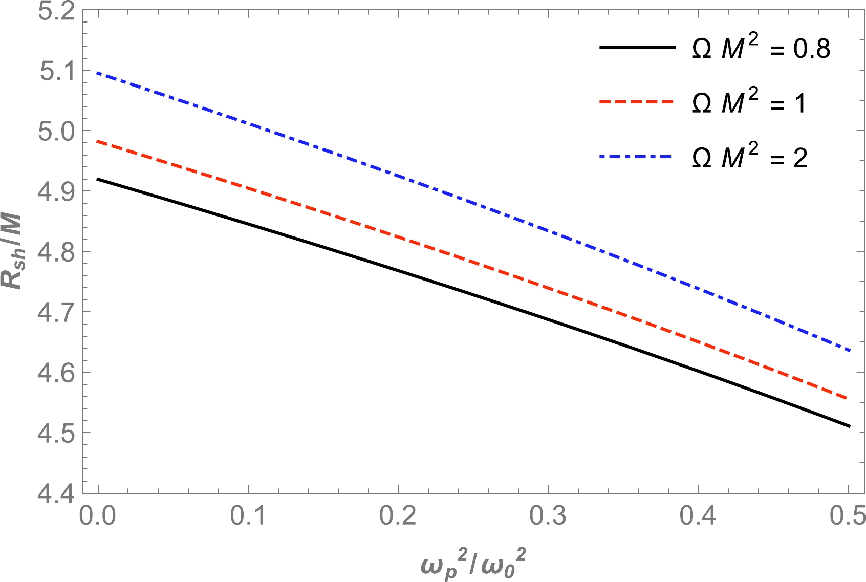
Figure 6. (color online) Dependence of the radius of the BH shadow on the plasma frequency for different values of the parameter
$\Omega M^2$ .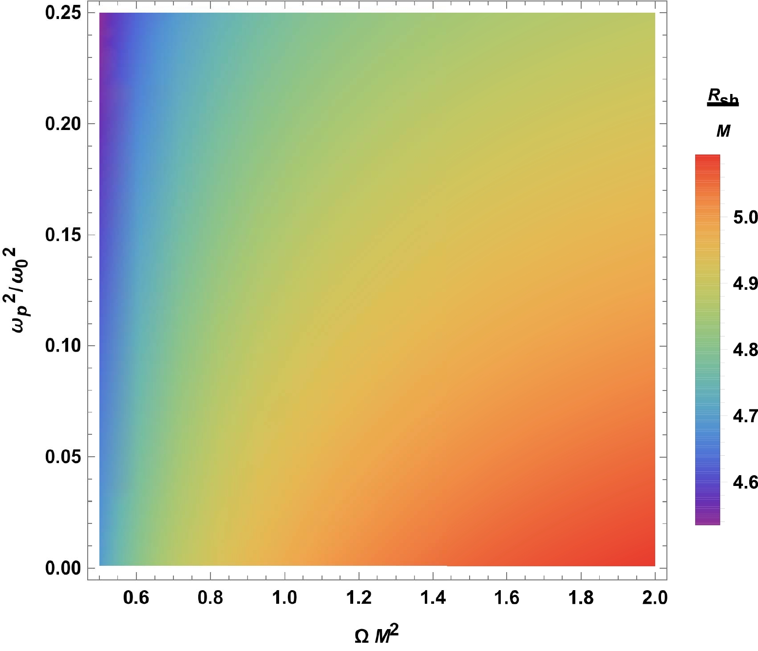
Figure 7. (color online) Color map indicating the strong dependence of the radius of the BH shadow on the parameter
$\Omega M^2$ .Now, we consider the assumption that Sgr A* and M87* are spherically symmetric static objects in HL gravity, although the observation obtained by the EHT collaboration does not support this assumption. However, we attempt to theoretically explore the lower limits of the KS parameter in HL spacetime using the data provided by the EHT collaboration. The spacetime metric has only one parameter Ω. Therefore, we choose plasma frequency as the second parameter for the constraint. We can use the observational data provided by the EHT collaboration regarding the shadows of the supermassive BHs Sgr A* and M87* to constrain the two parameters Ω and
$ \omega_p/\omega $ . The angular diameter$\theta_{\rm M87*}$ of the BH shadow, the distance from Earth, and the mass of the BH at the center of M87* are$\theta_{\rm M87*} = 42 \pm 3 ~ {\rm \mu \, as}$ ,$D = 16.8 \pm 0.8~ {\rm M pc}$ , and$M_{\rm M87*} = 6.5 \pm 0.7 \times 10^9 M_{\odot}$ [27], respectively. For Sgr A*, the data provided by the EHT collaboration are$\theta_{\rm Sgr A*} = 48.7 \pm 7 \mu$ $D = 8277 \pm 9 \pm 33~ {\rm pc}$ , and$M_{\rm Sgr A*} = 4.297 \pm 0.013 \times 10^6 M_{\odot}$ (VLTI) [98]. Using this information on BH shadows, we can roughly calculate the diameter of the shadow caused by the BH per unit mass with the following equation:$ d_{\rm sh} = \frac{D\theta}{M}\ . $

(30) From the expression
$d_{\rm sh} = 2R_{\rm sh}$ , we may now easily derive an expression for the diameter of the BH shadow:$d^{\rm M87*}_{\rm sh} = (11 \pm 1.5)M$ for M87* and$d^{\rm Sgr*}_{\rm sh} = (9.5 \pm 1.4)M$ for Sgr A*. Using EHT data, we can find the lower limits on the parameters Ω and$ \omega^2_{p}/\omega^2_0 $ for the supermassive BHs at the centers of the galaxies Sgr A* and M87*. This is represented numerically in Fig. 8.
Figure 8. Lower values of the parameters
$\Omega$ and$\omega^2_{p}/\omega^2_0$ for the supermassive BHs in the galaxies M87* and Sgr A*. We set$M=1$ in the both panels. -
In this section, we explore the optical properties of compact objects in HL gravity using the gravitational weak lensing effect. For a weak-field approximation, we can use the following standard notation for the metric tensor [75, 81]:
$ g_{\alpha \beta} = \eta_{\alpha \beta}+h_{\alpha \beta}\ , $

(31) where
$ \eta_{\alpha \beta} $ and$ h_{\alpha \beta} $ refer to the expressions for Minkowski spacetime and the perturbation gravity field describing HL theory, respectively. The following properties are required for$ \eta_{\alpha \beta} $ and$ h_{\alpha \beta} $ $ \begin{aligned}[b]& \eta_{\alpha \beta} = {\rm diag}(-1,1,1,1)\ , \\ & h_{\alpha \beta} \ll 1, h_{\alpha \beta} \rightarrow 0 ~~{\rm under}~~ x^{\alpha}\rightarrow \infty \ ,\\& g^{\alpha \beta} = \eta^{\alpha \beta}-h^{\alpha \beta},~~ h^{\alpha \beta} = h_{\alpha \beta}. \end{aligned}$

(32) Uniform and non-uniform plasma frequencies are renamed as
$ \omega_p $ and$ \omega_c $ , respectively. Furthermore, all graphs are corrected.Using the fundamental equation, we can obtain an expression for the angle of deflection around a compact object in HL gravity [75]:
$ \hat{\alpha }_{b} = \frac{1}{2}\int_{-\infty}^{\infty}\frac{b}{r}\left(\frac{{\rm d}h_{33}}{{\rm d}r}+\frac{1}{1-\omega^2_p/ \omega^2}\frac{{\rm d}h_{00}}{{\rm d}r}-\frac{K_e}{\omega^2-\omega^2_p}\frac{{\rm d}N}{{\rm d}r} \right){\rm d}z\ , $

(33) where ω and
$ \omega_{p} $ are known as quantities representing the photon and plasma frequencies, respectively. We expand the lapse function$ f(r) $ into a Taylor series owing to the difficulty of performing direct calculations on$ f(r) $ . We may rewrite the line element (1) in the form$ {\rm d}s^2 \approx {\rm d}s^2_0+\left(\frac{2 M}{r}-\frac{2 M^2}{r^4 \Omega }\right){\rm d}t^2 +\left(\frac{2 M}{r}-\frac{2 M^2}{r^4 \Omega }\right){\rm d}r^2\ , $

(34) where
${\rm d}s^2_0 = -{\rm d}t^2+{\rm d}r^2+r^2({\rm d}\theta^2+\sin^2\theta {\rm d}\phi^2)$ .Now, we can easily find the components
$ h_{\alpha \beta} $ of metric tensor perturbations in Cartesian coordinates in the form$ h_{00} = \frac{2 M}{r}-\frac{2 M^2}{r^4 \Omega } $

(35) $ h_{ik} = \left(\frac{2 M}{r}-\frac{2 M^2}{r^4 \Omega }\right)n_i n_k $

(36) $ h_{33} = \left(\frac{2 M}{r}-\frac{2 M^2}{r^4 \Omega}\right) \cos^2\chi \ , $

(37) where
$ \cos^2\chi = z^2/(b^2+z^2) $ , and$ r^2 = b^2+z^2 $ . The derivatives of$ h_{00} $ and$ h_{33} $ by the radial coordinate are defined as$ \frac{{\rm d}h_{00}}{{\rm d}r} = \frac{8 M^2}{r^5 \Omega }-\frac{2 M}{r^2}\ , $

(38) $ \frac{{\rm d}h_{33}}{{\rm d}r} = \frac{12 M^2 z^2}{r^7 \Omega }-\frac{6 M z^2}{r^4}\ . $

(39) We can write the following expression for the deflection angle [80]:
$ \hat{\alpha_b} = \hat{\alpha_1}+\hat{\alpha_2}+\hat{\alpha_3}\ , $

(40) with
$ \begin{aligned}[b] \hat{\alpha_1} =& \frac{1}{2}\int_{-\infty}^{\infty} \frac{b}{r}\frac{{\rm d}h_{33}}{{\rm d}r}{\rm d}z\ ,\\ \hat{\alpha_2} =& \frac{1}{2}\int_{-\infty}^{\infty} \frac{b}{r}\frac{1}{1-\omega^2_p/ \omega^2}\frac{{\rm d}h_{00}}{{\rm d}r}{\rm d}z\ ,\\ \hat{\alpha_3} = & \frac{1}{2}\int_{-\infty}^{\infty} \frac{b}{r}\left(-\frac{K_e}{\omega^2-\omega^2_p}\frac{{\rm d}N}{{\rm d}r} \right){\rm d}z\ . \end{aligned} $

(41) Now, we check and evaluate the deflection angle for different plasma density distributions.
-
In this subsection, the gravitational deflection angle around compact objects in HL gravity with its parameter in the presence of a uniform plasma can be written as the sum [80]
$ \hat{\alpha}_{\rm uni} = \hat{\alpha}_{{\rm uni}1}+\hat{\alpha}_{{\rm uni}2}+\hat{\alpha}_{{\rm uni}3}. $

(42) From Eqs. (37), (40), and (41), we may easily obtain the expression for the deflection angle around compact objects in HL gravity in a uniform plasma medium as
$ \hat{\alpha}_{\rm uni} = \frac{2 M}{b}-\frac{3 \pi M^2}{8 b^4 \Omega }+\left(\frac{2 M}{b}-\frac{3 \pi M^2}{2 b^4 \Omega }\right)\frac{\omega^2}{\omega^2-\omega^2_p}. $

(43) Using the above equation, we plot the dependence of the angle of deflection on the impact parameter b for different values of the parameter Ω,
$ \omega^2_{p}/\omega^2 $ , in the spacetime of KS gravity, which is presented in Fig. 9. Moreover, we explore the dependence of deflection angle on plasma parameters in Fig. 10 and the Ω parameter in Fig. 11.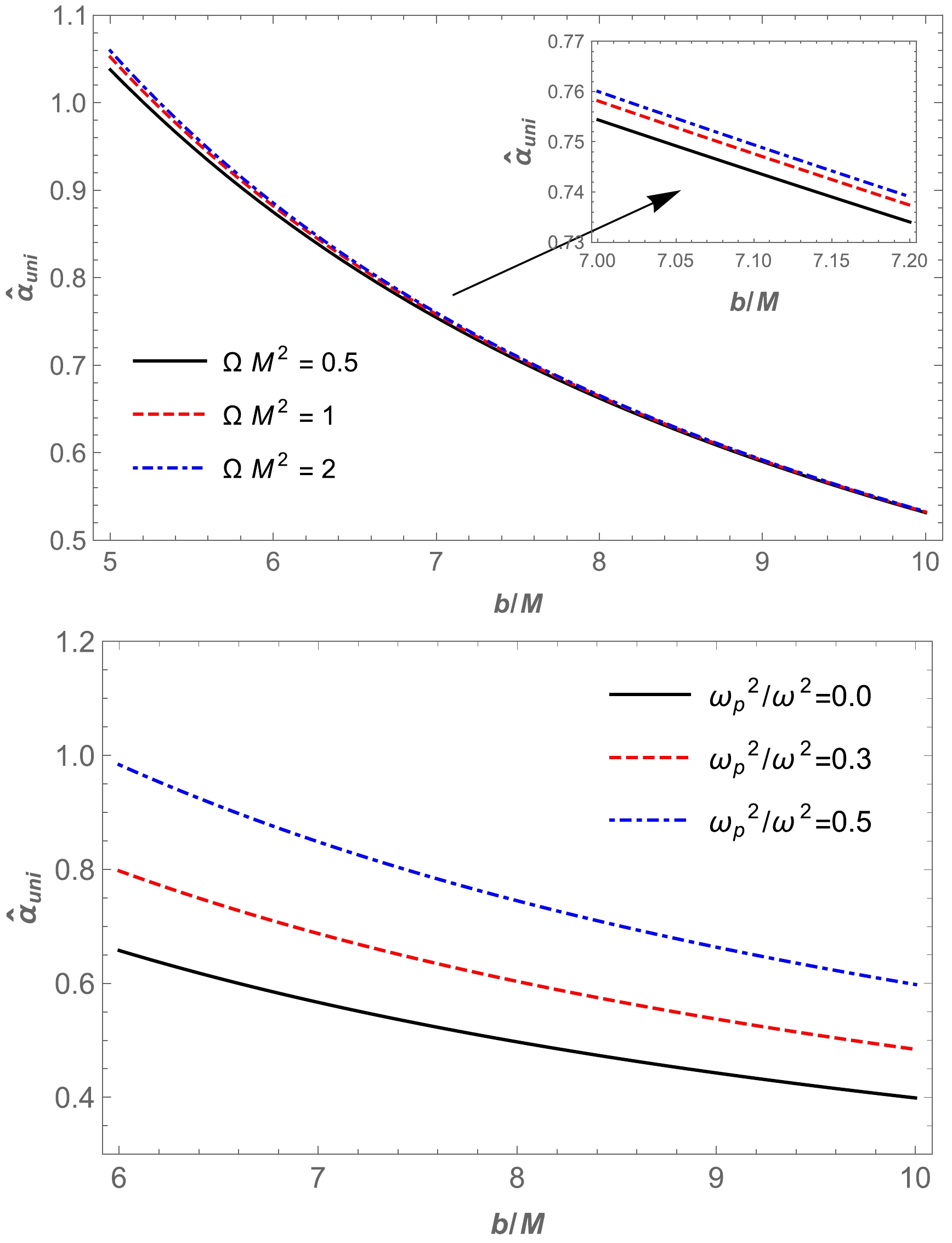
Figure 9. (color online) Dependence of the deflection angle
$\hat{\alpha}_{\text{uni}}$ on the impact parameter b for different values of the parameter$\Omega M^2 $ (upper panel) and plasma medium (bottom panel).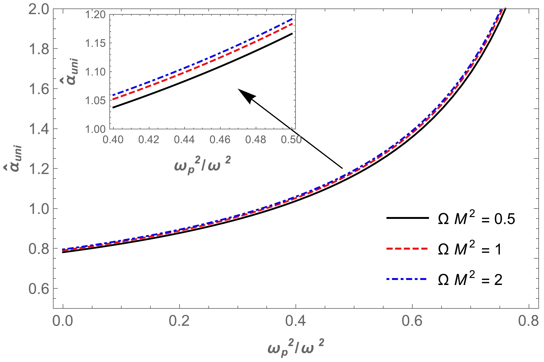
Figure 10. (color online) Dependence of the deflection angle
$\hat{\alpha }_{\text{uni}}$ on plasma parameters for the fixed value of the impact parameter$b = 5M$ .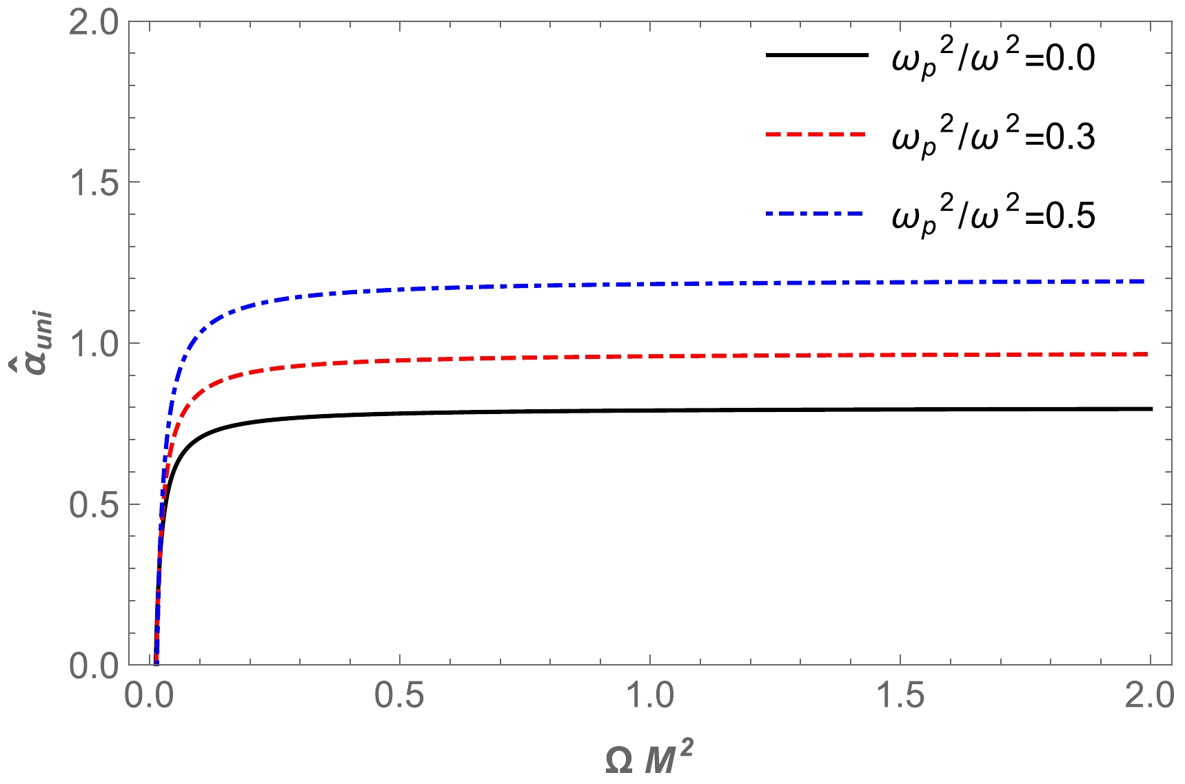
Figure 11. (color online) Dependence of the deflection angle
$\hat{\alpha }_{\text{uni}}$ on the parameter$\Omega M^2$ for the fixed value of the impact parameter$b = 5M$ . -
In this part of our current analysis, we consider a non-singular isothermal sphere (SIS), which is the most favorable model for understanding peculiar features of gravitational weak lensed photons around BHs. Generally, an SIS is a spherical gas cloud with a singularity located at its center, where the density tends to infinity. The density distribution of an SIS is given by [75]
$ \rho(r) = \frac{\sigma^2_{\nu}}{2\pi r^2}\ , $

(44) where
$ \sigma^2_{\nu} $ refers to a one-dimensional velocity dispersion. The plasma concentration has the following analytic expression [75]$ N(r) = \frac{\rho(r)}{k m_p}\ , $

(45) where
$ m_p $ is the proton mass, and k is a dimensionless constant coefficient generally associated with the dark matter universe. The plasma frequency is$ \omega^2_e = K_e N(r) = \frac{K_e \sigma^2_{\nu}}{2\pi k m_p r^2}\ . $

(46) Now, we explore the non-uniform plasma (SIS) effect on the deflection angle in the spacetime of an HL BH. We may write the expression for the deflection angle around a BH in HL gravity with the KS parameter as [80]
$ \hat{\alpha}_{\rm SIS} = \hat{\alpha}_{{\rm SIS}1}+\hat{\alpha}_{{\rm SIS}2}+\hat{\alpha}_{{\rm SIS}3} \ . $

(47) Combining Eqs. (37), (41), and (47), the deflection angle can be expressed in the following form:
$ \begin{aligned}[b] \hat{\alpha}_{\rm SIS} =& \frac{4 M}{b}-\frac{4 \omega _c^2 M^2}{\pi \omega ^2 b}+\frac{16 \omega _c^2 M^3}{3 \pi \omega ^2 b^3}\\&-\frac{15 \pi M^2}{8 b^4 \Omega }-\frac{5 \omega _c^2 M^4}{\omega ^2 b^6 \Omega }\ .\end{aligned} $

(48) These calculations introduce a supplementary plasma constant
$ \omega^2_c $ , which has the following analytic expression [81]:$ \omega^2_c = \frac{K_e \sigma^2_{\nu}}{2\pi k m_p R^2_S}\ . $

(49) Using Eq. (48), we construct graphs for the dependence of the angle of deflection on the impact parameter b for different values of the parameters Ω and
$ \omega^2_{c}/\omega^2 $ for non-uniform plasma medium in HL spacetime, as shown in Fig. 12. Then, we demonstrate the dependence of the angle of deflection of a light ray around a BH in the presence of a non-uniform plasma in Figs. 13 and 14.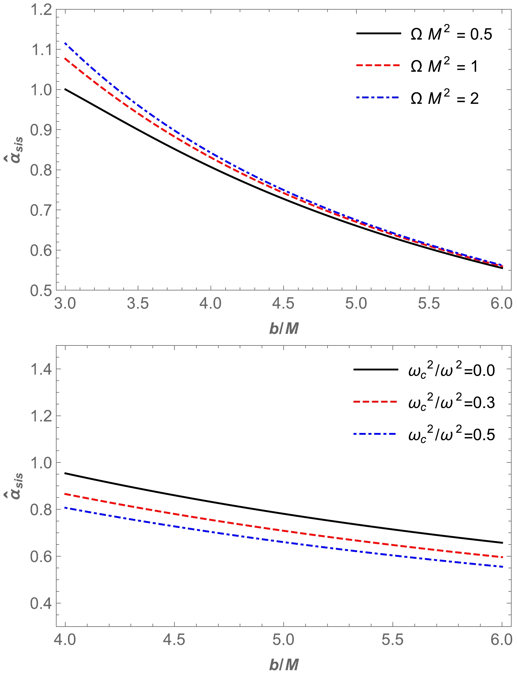
Figure 12. (color online) Dependence of the deflection angle
$\hat{\alpha }_{\text{sis}}$ on the impact parameter for different values of the parameter$\Omega M^2$ (upper panel) and plasma parameters (lower panel).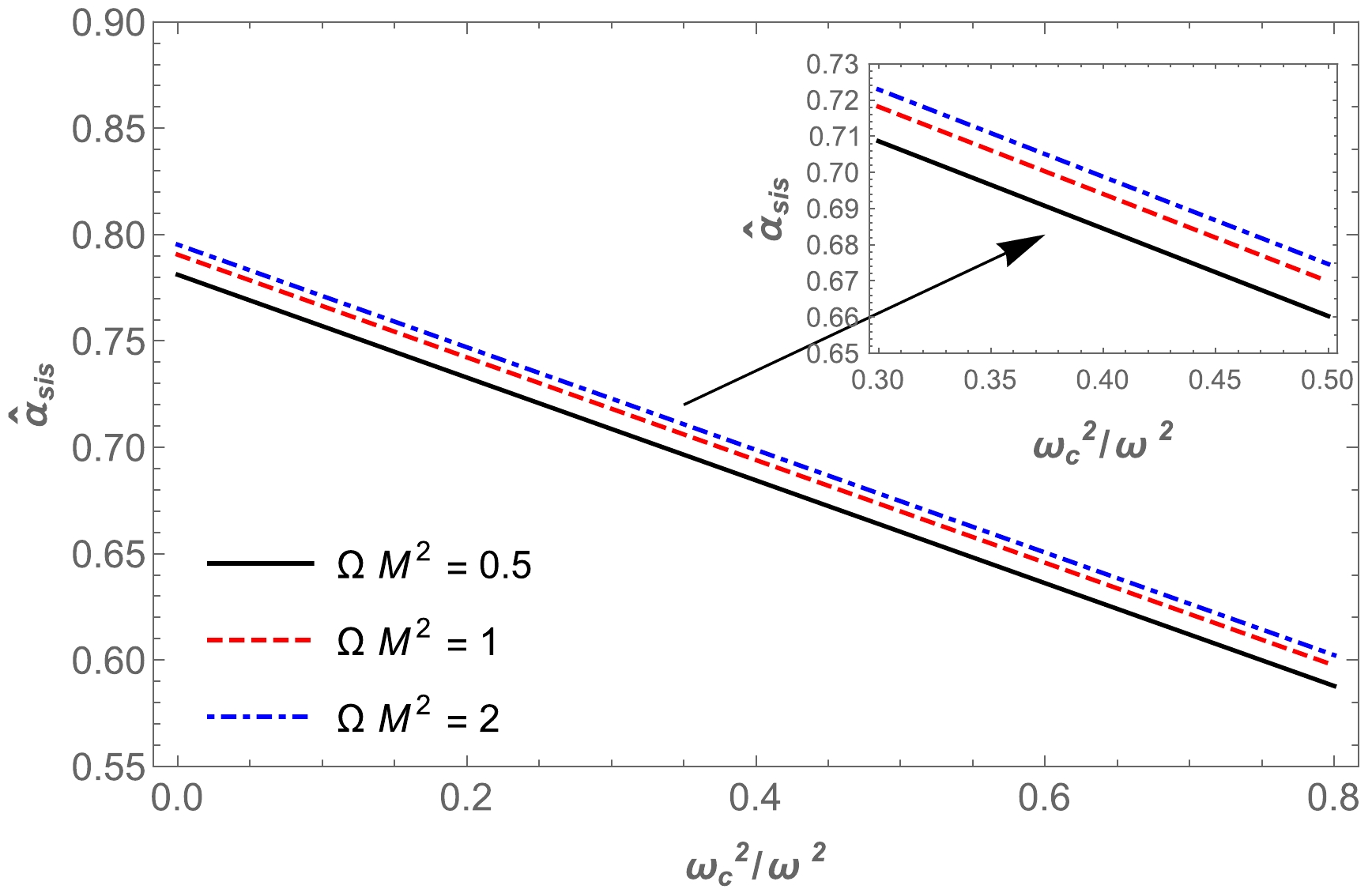
Figure 13. (color online) Dependence of the deflection angle
$\hat{\alpha }_{\text{sis}}$ on plasma for the fixed value of the impact parameter$b = 5M$ .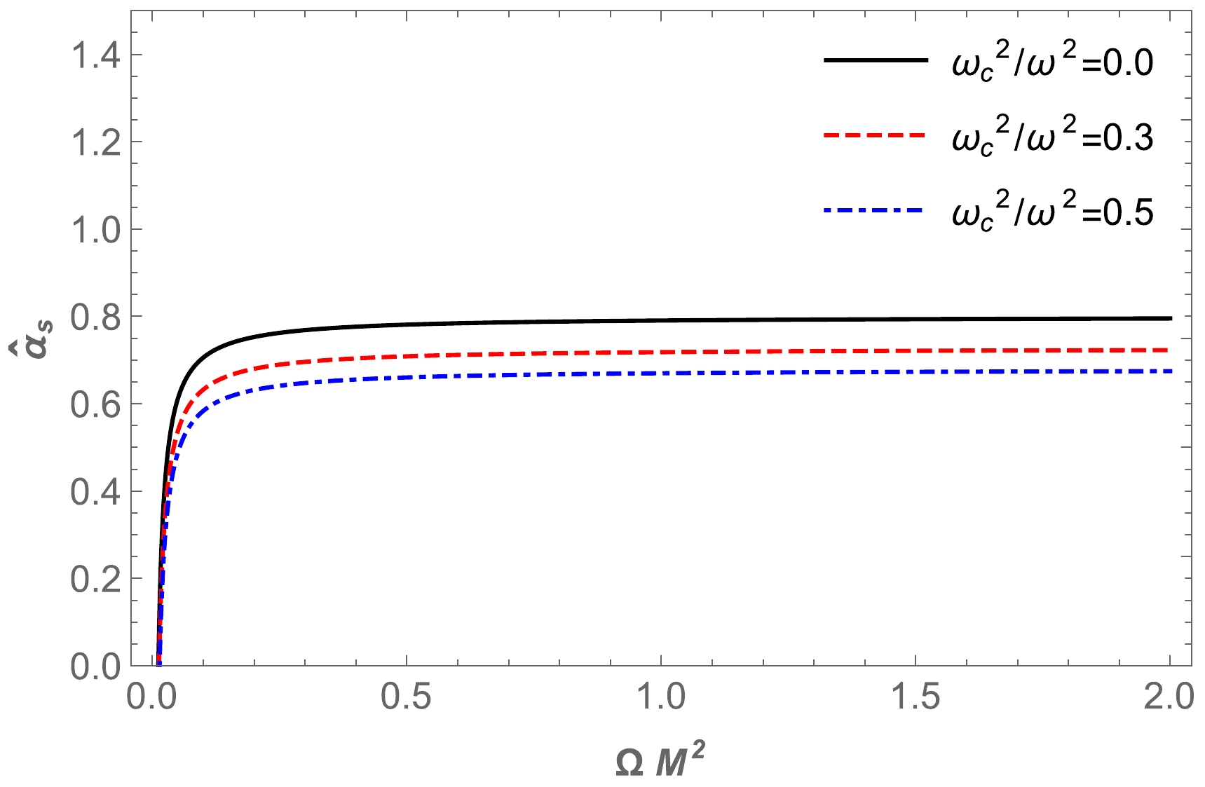
Figure 14. (color online) Dependence of the deflection angle
$\hat{\alpha }_{\text{sis}}$ on the parameter$\Omega M^2$ for the fixed value of the impact parameter$b = 5M$ .In addition, we compare the different effects of plasma on the HL BH deflection angle with gravity, as shown in Fig. 15.
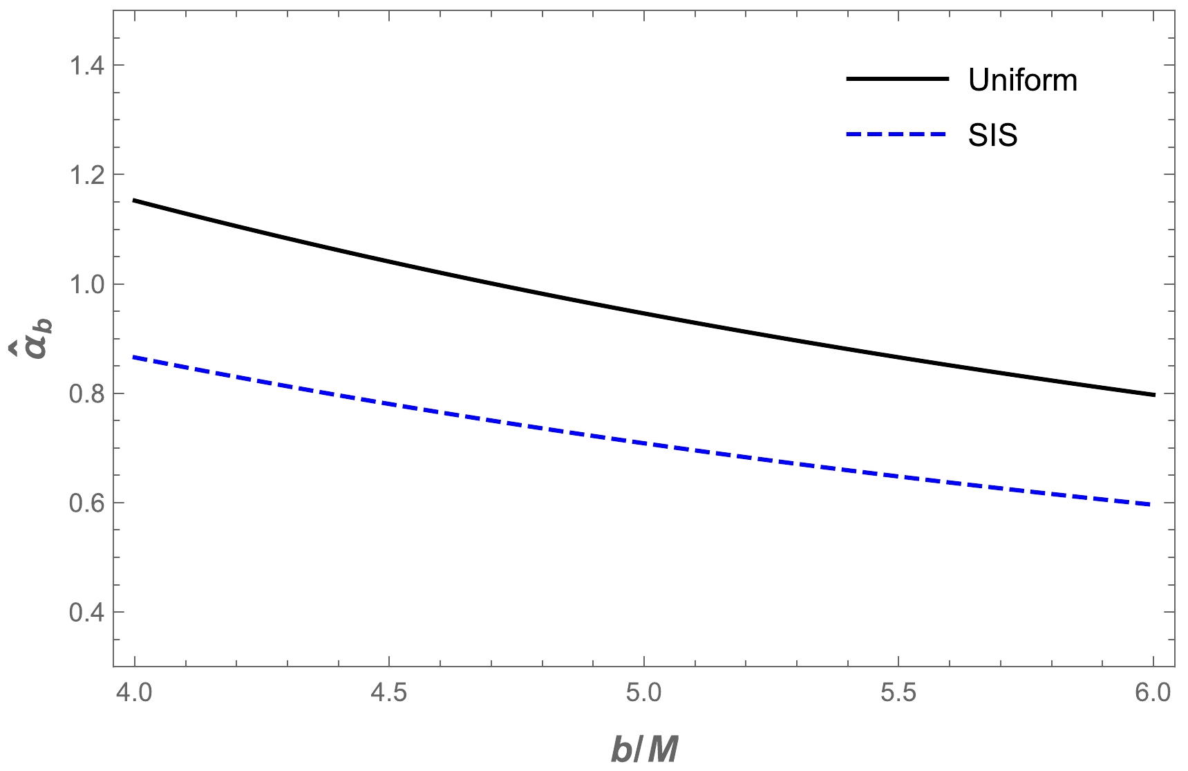
Figure 15. (color online) Dependence of the deflection angle
$\hat{\alpha }_{b}$ on the impact parameter. -
Now, we explore the brightness of an image in the presence of plasma through the deflection angle of light rays around a BH in HL gravity. Using the lens equation, we can express the combination of light angles around the BH in HL gravity (
$ \hat{\alpha} $ , θ, and β) [77, 81, 99] as$ \begin{align} \theta D_{s} = \beta D_{s}+\hat{\alpha_b}D_{ds}\ , \end{align} $

(50) where
$D_{s}$ ,$D_{d}$ , and$D_{ds}$ are the distances from the source to the observer, from the lens to the observer, and from the source to the lens, respectively, and θ and β refer to the angular position of the image and source. From the above equation, we can rewrite the equation for β as$ \begin{align} \beta = \theta -\frac{D_{ds}}{D_{s}}\frac{\xi(\theta)}{D_{d}}\frac{1}{\theta}\ , \end{align} $

(51) where
$ \xi(\theta) = |\hat{\alpha}_b|b $ and$b = D_{d}\theta$ have been used in [81]. If the shape of the image looks like a ring, it is defined as Einstein's ring, and the radius of Einstein's ring is$R_s = D_{d}\theta_E$ . The angular part$ \theta_E $ due to spacetime geometry between the images of the source in a vacuum [100] can be written as$ \begin{align} \theta_E = \sqrt{2R_s\frac{D_{ds}}{D_dD_s}}\ . \end{align} $

(52) Now, we explore the expression for the magnification of brightness [100].
$ \begin{align} \mu_{\Sigma} = \frac{I_\mathrm{tot}}{I_*} = \underset{k}\sum\bigg|\bigg(\frac{\theta_k}{\beta}\bigg)\bigg(\frac{{\rm d}\theta_k}{{\rm d}\beta}\bigg)\bigg|, \quad k = 1,2, \cdot \cdot \cdot , j\ , \end{align} $

(53) where
$ I_* $ and$ I_\mathrm{tot} $ are the unlensed brightness of the source and the total brightness of all images, respectively. The expressions for the magnification of the source are written in the following form [100]:$ \begin{align} \mu^\mathrm{pl}_\mathrm+ = \frac{1}{4}\bigg(\frac{x}{\sqrt{x^2+4}}+\frac{\sqrt{x^2+4}}{x}+2\bigg)\ , \end{align} $

(54) $ \begin{align} \mu^\mathrm{pl}_\mathrm- = \frac{1}{4}\bigg(\frac{x}{\sqrt{x^2+4}}+\frac{\sqrt{x^2+4}}{x}-2\bigg)\ , \end{align} $

(55) where
$ x = {\beta}/{\theta_E} $ is a dimensionless quantity [81], and$ \mu_{+}^{\mathrm{pl}} $ and$ \mu_{-}^{\mathrm{pl}} $ are the images. Using Eqs. (54) and (55), we can obtain the formula for the total magnification in the form$ \begin{align} \mu^\mathrm{pl}_\mathrm{tot} = \mu^\mathrm{pl}_++\mu^\mathrm{pl}_- = \frac{x^2+2}{x\sqrt{x^2+4}}\ . \end{align} $

(56) Next, we investigate the magnification in the presence of plasma in the BH environment with different distributions of plasma: (i) uniform and (ii) non-uniform cases.
-
In this subsection, we explore the effect of uniform plasma on the magnification of an image in HL gravity theory, and we write expressions for the total magnification
$\mu^{\rm pl}_{\rm tot}$ and angle$(\theta^{\rm pl}_{E})_{\rm uni}$ as$ \mu^{\rm pl}_{\rm tot} = \mu^{\rm pl}_++\mu^{\rm pl}_- = \dfrac{x^2_{\rm uni}+2}{x_{\rm uni}\sqrt{x^2_{\rm uni}+4}}\ , $

(57) and
$ (\theta^{\rm pl}_{E})_{\rm uni} = \theta_E\sqrt{\frac{1}{2}\left(\left( 1-\frac{3 \pi M}{4 b^3 \Omega }\right)\frac{1}{1-\dfrac{\omega^2_p}{\omega^2}}-\frac{3 \pi M}{16 b^3 \Omega }+1\right)}\ , $

(58) where
$x_{\rm uni}$ is defined as$ \begin{aligned}[b] x_{\rm uni} =& \frac{\beta}{(\theta^{\rm pl}_E)_{\rm uni}} = \\ = & \frac{x_0}{\sqrt{\dfrac{1}{2}\left(\left( 1-\dfrac{3 \pi M}{4 b^3 \Omega }\right)\frac{1}{1-\dfrac{\omega^2_p}{\omega^2}}-\dfrac{3 \pi M}{16 b^3 \Omega }+1\right)}} \end{aligned} $

(59) where
$ x_0 = \beta/\theta_E $ , and we can write the magnifications of the image as$ (\mu^{\rm pl}_+)_{\rm uni} = \frac{1}{4}\left(\dfrac{x_{\rm uni}}{\sqrt{x^2_{\rm uni}+4}}+\dfrac{\sqrt{x^2_{\rm uni}+4}}{x_{\rm uni}}+2\right) $

(60) $ (\mu^{\rm pl}_-)_{\rm uni} = \frac{1}{4}\left(\dfrac{x_{\rm uni}}{\sqrt{x^2_{\rm uni}+4}}+\dfrac{\sqrt{x^2_{\rm uni}+4}}{x_{\rm uni}}-2\right) $

(61) The total magnification of the image in the presence of a plasma
$ \mu^\mathrm{pl}_\mathrm{tot} $ in HL gravity with its parameter is represented in Figs. 16 and 17. A plot of the dependence of the total magnification on$ x_{0} $ in the presence of uniform plasma for fixed values of the parameter Ω is demonstrated in Fig. 18.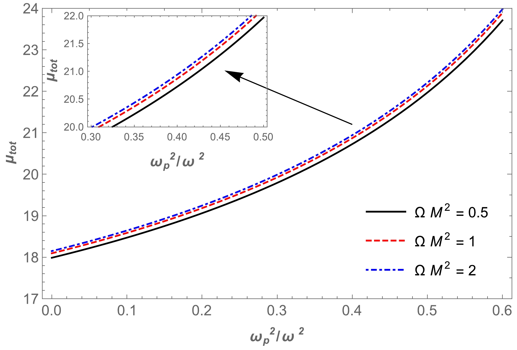
Figure 16. (color online) Dependence of the total magnification
$\mu_{\rm tot}$ on the plasma parameter for different values of the parameter$\Omega M^2$ corresponding to the fixed value of the impact parameter$b = 5M$ .
Figure 17. (color online) Dependence of the total magnification
$\mu_{\rm tot}$ on the parameter$\Omega M^2$ for different values of the plasma parameter corresponding to the fixed value of the impact parameter$b = 5M$ . -
Here, we study the effect of non-uniform plasma (as SIS medium) on magnification, which can be written as
$ (\mu^{\rm pl}_{\rm tot})_{\rm SIS} = (\mu^{\rm pl}_+)_{\rm SIS}+(\mu^{\rm pl}_-)_{\rm SIS} = \dfrac{x^2_{\rm SIS}+2}{x_{\rm SIS}\sqrt{x^2_{\rm SIS}+4}}\ , $

(62) with
$ (\mu^{\rm pl}_+)_{\rm SIS} = \frac{1}{4}\left(\dfrac{x_{\rm SIS}}{\sqrt{x^2_{\rm SIS}+4}}+\dfrac{\sqrt{x^2_{\rm SIS}+4}}{x_{\rm SIS}}+2\right)\ , $

(63) $ (\mu^{\rm pl}_-)_{\rm SIS} = \frac{1}{4}\left(\dfrac{x_{\rm SIS}}{\sqrt{x^2_{\rm SIS}+4}}+\dfrac{\sqrt{x^2_{\rm SIS}+4}}{x_{\rm SIS}}-2\right)\ , $

(64) and
$ \begin{aligned}[b] x_{\rm SIS} =& \frac{\beta}{(\theta^{\rm pl}_E)_{\rm SIS}} \\ = & \frac{x_0}{\sqrt{1-\dfrac{5 \omega_c^2 M^3}{4 \omega^2 b^5 \Omega }-\dfrac{15 \pi M}{32 b^3 \Omega }+\dfrac{4 \omega_c^2 M^2}{3 \pi \omega^2 b^2}-\dfrac{\omega_c^2 M}{\pi \omega^2 }}}\ . \end{aligned}$

(65) Using Eq. (62), we can find the dependence of total magnification on the plasma parameter. With the increase in the plasma parameter, magnification decreases, as represented in Fig. 19. Moreover, a plot of the dependence of total magnification on
$ x_{0} $ in the presence of plasma for fixed values of the parameter Ω is presented in Fig. 20. Finally, in Fig. 21, we present a comparison of these two cases, that is, for uniform and non-uniform plasma distributions.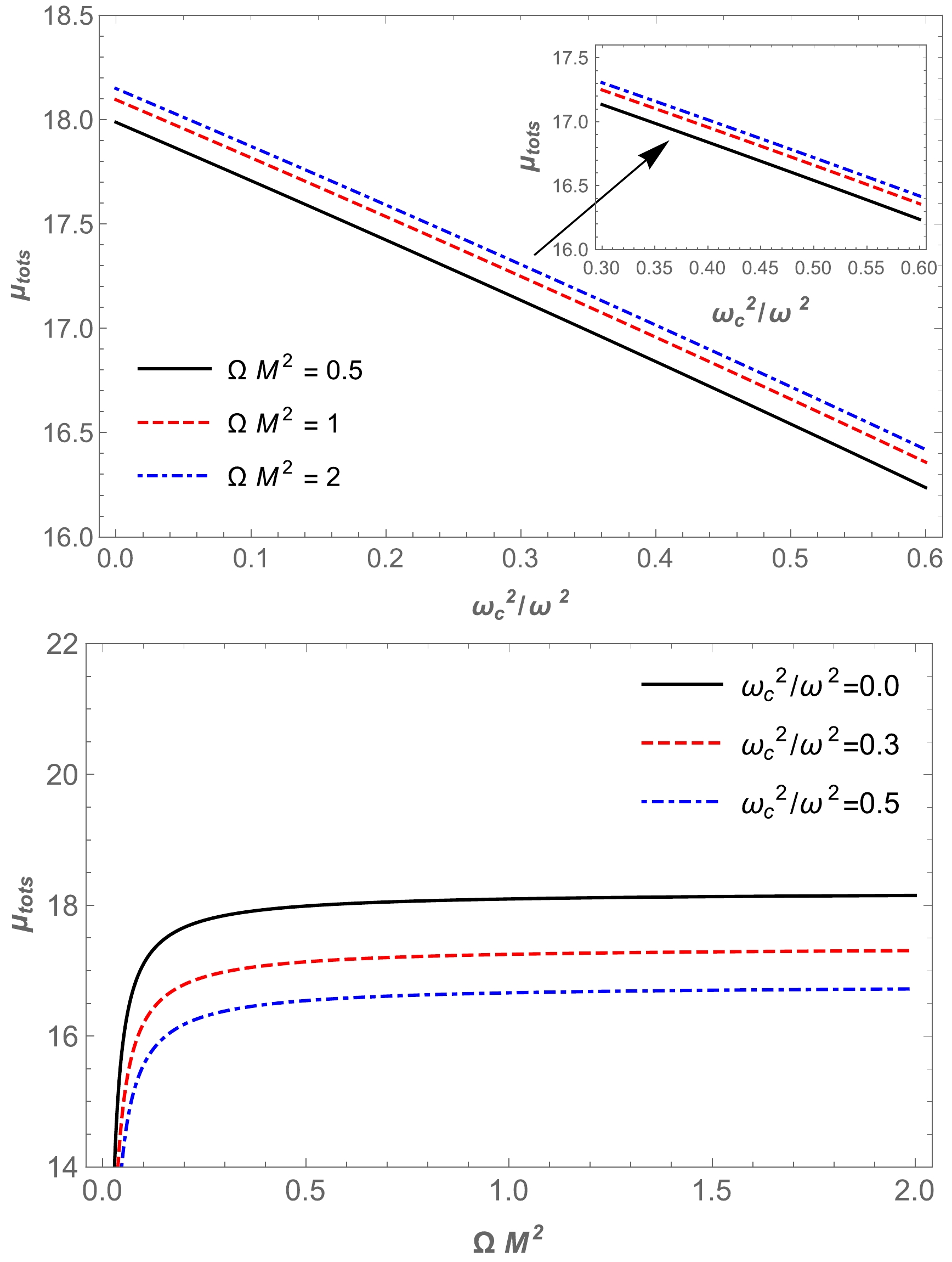
Figure 18. (color online) Total magnification of the images as a function of non-uniform plasma. Here, the impact parameter is set as
$b = 5M$ .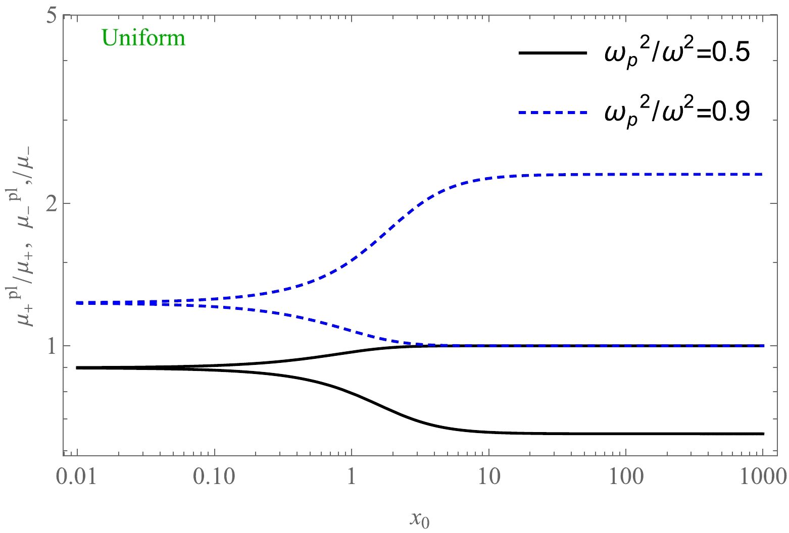
Figure 19. (color online) Image magnification in the presence of uniform plasma. The fixed parameters used are
$M=1$ ,$b=3M$ , and$\Omega M^2=0.5$ .
Figure 20. (color online) Image magnification in the presence of an SIS. The fixed parameters used are
$M=1$ ,$b=3M$ , and$\Omega M^2=0.5$ .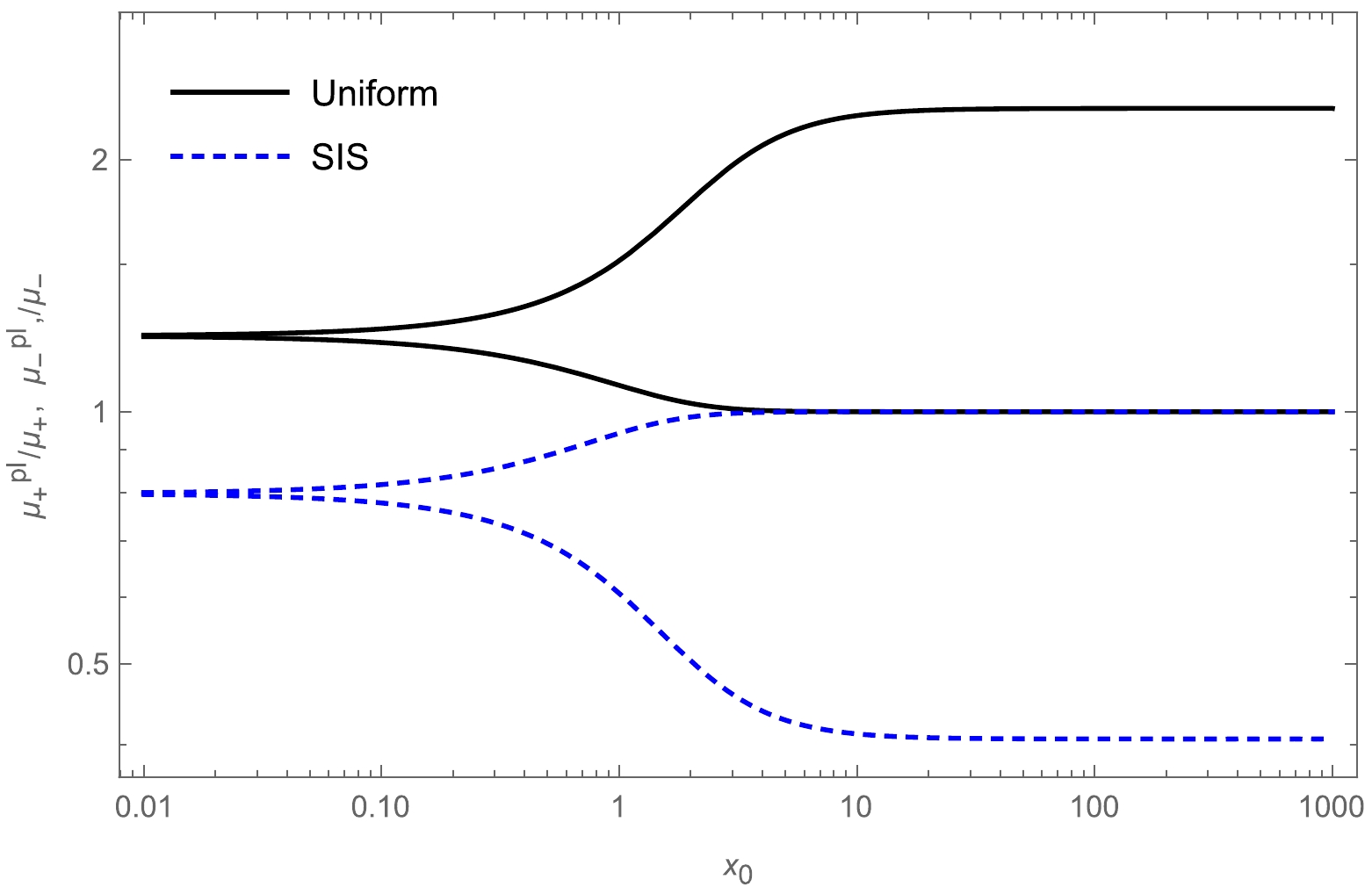
Figure 21. (color online) Image magnifications in the presence of uniform plasma and an SIS. The fixed parameters used are
$M=1$ ,$b=3M$ ,$\dfrac{\omega^2_{p}}{\omega^2}=0.5$ ,$\dfrac{\omega^2_c}{\omega^2}=0.5$ , and$\Omega M^2=0.5$ . -
In this study, we discuss particle motion around a BH and the plasma effect on the optical properties of the BH in HL space-time with the KS parameter. From our research, we can summarize our main results as follows:
● We extensively study particle motion around a KS compact object and discuss the dependence of the effective potential of a massive particle on the radial coordinate for different values of the Hořava parameter Ω, the results of which are presented in Fig. 1.
● Using effective potential, the ISCO is investigated for massive particles orbiting a BH in HL gravity, and the obtained results are presented in Fig. 3. The derived results show that the influence of the Hořava parameter shifts the ISCO toward the central object.
● We also study the effects of plasma on the radius of the photon sphere in a plasma medium and find that the radius of the photon sphere decreases with the Hořava parameter Ω, as shown in Fig. 4.
● Furthermore, we investigate the observable parameter, that is, the radius of the BH shadow. The size of the radius of the BH shadow decreases in the presence of the Hořava parameter, similar to the effect of plasma frequency. This is represented in Figs. 5, 6, and 7.
● In addition, we study one more optical property of a BH in HL gravity through light rays: gravitational weak lensing. Initially, we focus on the deflection angle of light rays around the BH in KS gravity in the presence of plasma (uniform and non-uniform cases) and find that the influence of uniform plasma on the deflection angle is greater than that in the non-uniform plasma case for fixed parameters of the BH in HL gravity.
● Finally, we investigate the magnification of an image using the deflection angle of light rays, which is shown in detail in Figs. 19 and 20. We compare the magnifications of the uniform and non-uniform cases, as shown in detail in Fig. 21.
● Because we demonstrate that the size of the shadow depends on the BH and gravity theory parameters, in the future, the obtained results can be applied to images of the Sgr A* and M 87* supermassive BHs to obtain constraints on the HL gravity parameters.
Additionally, the observational data of gravitational lensing in Refs. [101−104] may be further used to obtain constraints on the spacetime parameters of HL and estimate plasma characteristics.
-
MA, AA, and BA thank the Institute of Physics in Opava for the hospitality during their stay there.
Probing Hořava-Lifshitz gravity using particle and photon dynamics in the presence of plasma
- Received Date: 2023-04-16
- Available Online: 2023-07-15
Abstract: We study the particle motion around a black hole (BH) in Hořava-Lifshitz (HL) gravity with the Kehagias-Sfetsos (KS) parameter. First, the innermost stable circular orbit (ISCO) is obtained for massive particles around the BH in HL gravity. We find that the radii of the ISCOs decrease as the KS parameter decreases, meaning that the parameter


 DownLoad: