Echoes of axial gravitational perturbations in stars of uniform density

Compact objects, such as a neutron star or black hole, produce gravitational waves (GWs) triggered by metric perturbations. The dissipative process essentially features three stages: the initial burst, quasinormal mode (QNM) oscillations, and the late-time tail. In the initial burst stage, the system's dynamical properties are determined mainly by the initial conditions. In contrast, in the QNM and late-time tail stages, the process is primarily governed by the intrinsic nature of compact objects. For spherically symmetric metrics, the master equation can be simplified, and in the frequency domain, the radial sector can be expressed as a Schördinger type equation regarding a complex eigenfrequency ω. A variety of methods were proposed, and one is expected to extract valuable information on the underlying stars or black holes from the GW measurements [1−9]. The relevant studies in which analysis of observed quasinormal frequencies, known as QNM spectroscopy, was performed have gained considerable momentum recently [10−16].

Regarding black hole QNMs, the dynamic temporal evolution of the initial perturbations is usually explored at a given spatial point. However, it is more meaningful to study the GW propagation for the entire range of spatial coordinates, for instance, in the two-dimensional $ t-r_* $ coordinate space (where $r_*=\int {\rm d}r/\sqrt{fh}$ is the tortoise coordinate). In literature, many semi-analytic methods, such as the WKB approximation [17−23], continued fractional method [24, 25], asymptotic iteration method [26−29], and matrix method [30−34], among others [35−40], have been proposed. These approaches have been extensively adopted for evaluating black hole QNM frequencies ω. For star QNMs, however, they must be modified accordingly and often used in conjunction with the shooting method [41−47]. Nonetheless, the above approaches only concern the QNM oscillation stage, and therefore, they cannot be employed to address the entire process. In this regard, the finite difference method (FDM) is a suitable approach that can be used to provide a more general description of the dynamical evolution for given initial perturbations [48−53].

In practice, to implement the FDM, the boundary condition and initial conditions are often proposed on the axes of the Eddington-Finkelstein coordinates, $ \Psi(u,v= $ 0) = 0 and $ \Psi(u=0,v)=\Psi_0 $ (where $ u=t-r_* $ and $ v=t+r_* $), respectively. Assuming that the spacetime in the tortoise coordinate is mainly flat, so that the speed of light of the waveform $ c\sim 1 $, the boundary placed on $ u=0 $ is mostly in accordance with the causality that will never be attained by the initial perturbations assigned to the surface $ v=0 $. In practice, the assumption that $ c\sim 1 $has been clearly shown as a reasonable approximation in numerical calculations. In principle, however, it might be violated in the vicinity of the black hole. More specifically, although the above boundary condition is asymptotically correct, for a finite period, the initial perturbations might temporarily travel across the v axis. Thus, we propose an alternative approach as follows. The initial conditions are placed on the spatial surface$ t=0 $, and appropriate boundary conditions are adopted in accordance with the causality. For the black hole spacetime, free boundary conditions are implemented so that the initial perturbations will propagate as an ingoing wave toward the horizon and an outgoing wave toward spatial infinity. For the compact star spacetime, the free boundary condition will be adopted at the spatial infinity for the reason mentioned above, and the perturbations must vanish at the center of the star as the effective potential goes to infinity. Moreover, the junction condition in terms of a vanishing Wronkian is enforced at the star's surface. The proposed scheme is more flexible as it can be easily modified to adopt the case where the speed of light exceeds the unit. Therefore, it is considered in the present work to investigate the temporal profiles of both black holes and stars. The obtained results are illustrated in a two-dimensional evolution profile. In the case of black holes, it is found that the resulting ringdown waveforms are featured by the reflected and transmitted waves as the initial perturbations evolve and collide with the maximum of the effective potential. Meanwhile, in the case of compact stars, temporal evolutions may also be characterized by echoes. These echoes have largely been speculated to be associated with compact objects [54−57], such as black holes and wormholes, which has become an intriguing topic in recent years. Typically, their emergence is understood to be related to the existence of an effective potential well. Specifically, for the wormhole metric explored in Ref. [56], echoes are intuitively attributed to the potential well between the two maxima. Moreover, the echo's period is governed by twice the distance between the peaks. In the context of a black hole or other exotic compact objects, the period of the echoes is related to the distance between the maximum of the effective potential and the surface or inner boundary of the compact object [55]. More recently, it was pointed out that a discontinuity may also play such a role in triggering echoes [57]. For the present scenario, the echoes can be attributed to the repeated bouncing of the waveforms between the star's center and its surface.

The remainder of the paper is organized as follows. In the following section, we present the numerical schemes of the FDM and the associated von Neumann stability condition. In Section III, the obtained numerical results are discussed. Section IV presents the concluding remarks.

For the sake of simplicity, we consider the spherically symmetric spacetimes, whose metric possess the form

For the Schwarzschild black hole, we have

where $ M_S $ and $ r_p=2M_S $ are the mass and horizon of the black hole, respectively. The tortoise coordinate $r_*= \int {\rm d}r/ \sqrt{fh}$ reads $ r_*=r+r_S\log\left(\dfrac{r}{r_S}-1\right) $.

For the stars with uniform density $ \rho=\dfrac{3M_S}{4\pi r_b^3} $, where $ r_b $ is the radial coordinate of the star's surface, the metricis idential to Eq. (2) for the outside region $ r \ge r_b $. On the inside of the star ($ r<r_b $) [58],

For the tortoise coordinate, the constant of integration is chosen so that $ r_*(r=0)=0 $.

Using the method of seperation of variables, the axial gravitational perturbations are governed by [59]

At spatial infinity, the boundary condition dictates that waveform Ψ is a symptotic outgoing wave. For black holes, Ψ must be an asymptotic ingoing wave at the horizon. For stars, the wave function must be regular at the center of the star, and the junction conditions at the star's surface reads

if the effective potential is not divergent at the surface.

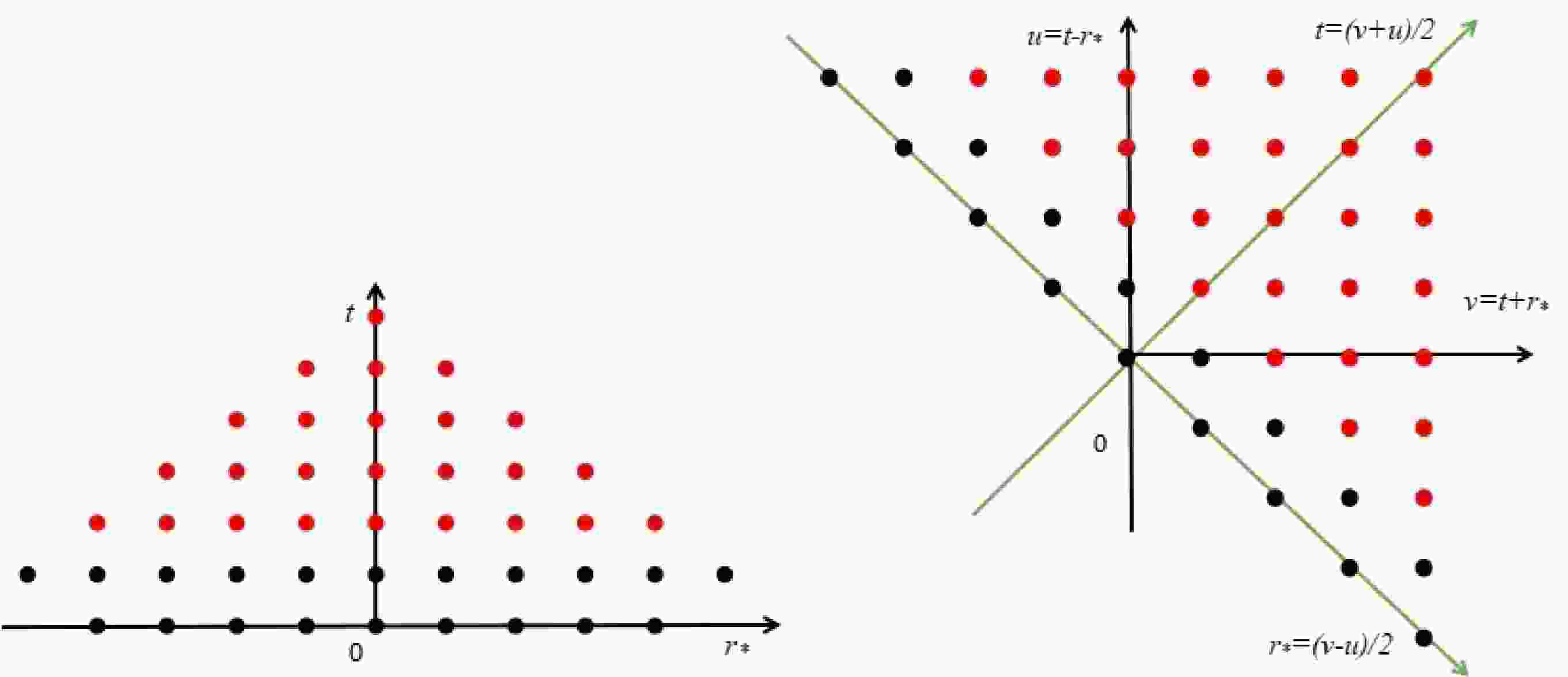
In the proposed scheme, as shown in the left plots of Figs. 1 and 2, the initial conditions are given at the spatial surface $ t=0 $, namely, $ \Psi(t=0) $ and $ \partial_t\Psi(t=0) $. Subsequently, the spacetime coordinates in$ r_* $and t are discretized, and the partial derivatives are approximated by first-order finite differences. Specifically, $t_i=t_0+{\rm i}\Delta t$, $ r_{*j}=r_{*0}+ j\Delta r_* $ , $ \Psi^i_j=\Psi(t=t_i,r_*=r_{*j}) $, and $V_j=V (r_*=r_{*j})$; the master equation (Eq. (4)) becomes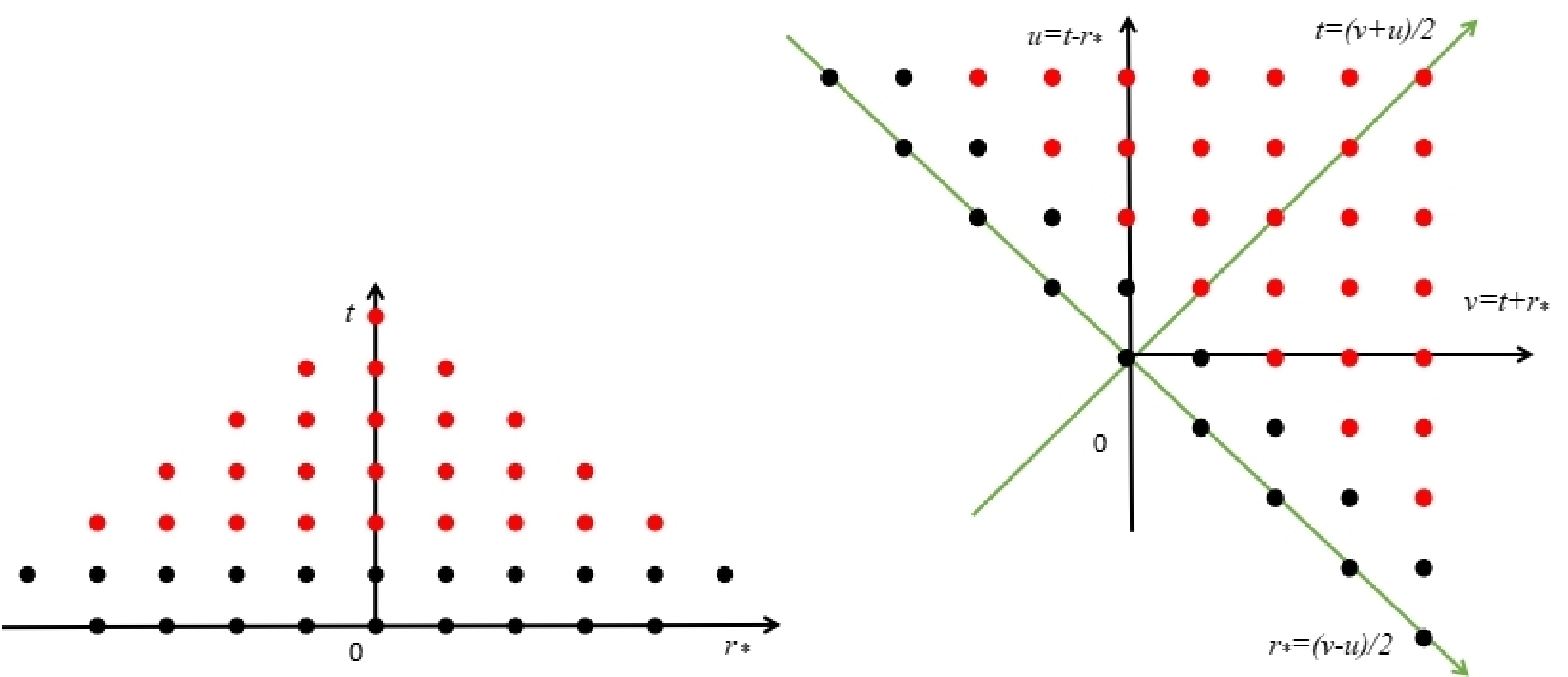

Figure 1.  (color online) Grid layouts of two FDM implementations in the case of a black hole. The left plot corresponds to the proposed scheme in $ (r_*, t) $ coordinates, and the right plot is that in the conventional $ (u, v) $ coordinates. The black points are the grids to which the initial conditions are assigned, and one uses the iteration process to evaluate the red points, as described in the text.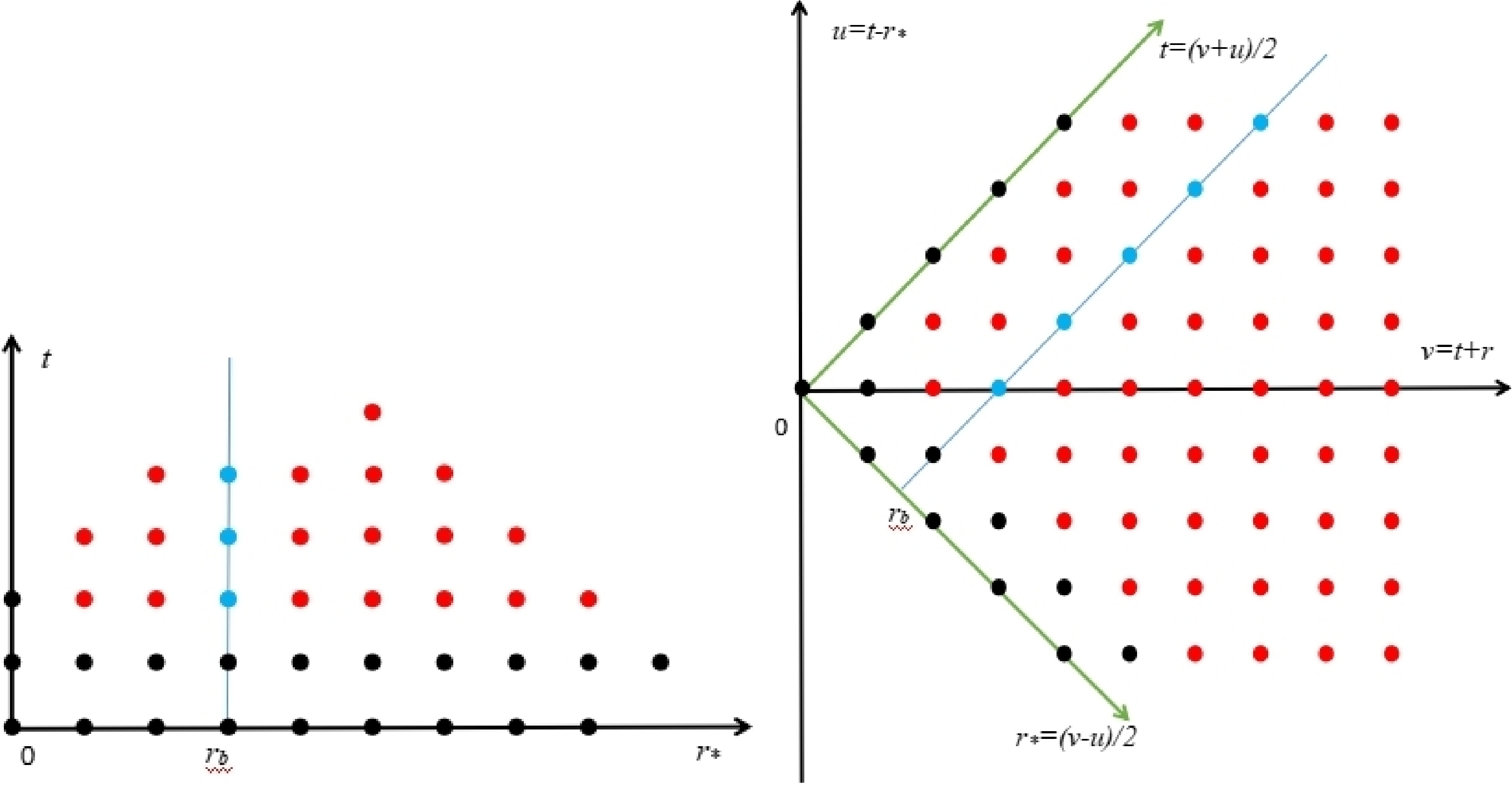

Figure 2.  (color online) The same as Fig. 1 but for the case of a star. Here, the light blue points correspond to the star's surface $ r=r_b $, which should be evaluated according to the iteration process is described in the text.

For the stars, the junction condition in Eq. (5) reads

where $ \Psi^i_{j_b-1}=\Psi_\text{inside}(r_*=r_{*0}+(j_b-1)\Delta r_*) $, $ \Psi^i_{j_b+1}= \Psi_\text{outside}(r_*=r_{*0}+(j_b+1)\Delta r_*) $, and $ \Psi^i_{j_b}=\Psi_\text{inside}(r_*=r_{*0}+ j_b\Delta r_*)=\Psi_\text{outside}(r_*=r_{*0}+j_b\Delta r_*) $, so that

where subscript b indicates that the grid is on the star's surface.

The temporal evolution is performed by iterating from both boundaries toward the center. Usually, Eq. (6) is utilized to determine the grid values for the next time step, except for those on the star's surface where the iteration formula would involve grids on both sides of the surface. For the latter case, Eq. (7) is considered instead to determine the value of the wave function on the surface; then, the calculation is resumed with Eq. (6). To avoid the von Neumann instability [51, 52], we choose $ \dfrac{\Delta t^2}{\Delta r_*^2}+ \dfrac{\Delta t^2}{4}V_\text{max}<1 $.

Alternatively, one can explore the problem in the Eddington-Finkelstein coordinates $ u=t-r_*, v=t+r_* $. The grid distributions are illustrated on the right of Figs. 1 and 2. Although the discretization of the master equation is carried out in a different coordinate system, as discussed below, it is noted that the essential difference from the conventional approach resides in the boundary conditions. Specifically, in the case of the black hole metric, the free boundary condition is adopted instead of assigning to the line $ v=0 $. In terms of the Eddington-Finkelstein coordinates, the master equation (Eq. (4)) can be rewritten as

Similarly, one denotes $v_i=v_0+{\rm i}\Delta v$, $u_j=u_0+{\rm i}\Delta u$, $ \Psi^i_j=\Psi(v_i, u_j) $, and $ V^i_j=V(v_i,u_j) $; therefore, the discritized equation is found to be

where $ \Delta v=\Delta u=\Delta $is considered. The iteration can be carried out as the value of a grid point is determined by three grid points to the immediate west, south, and south-west of the grid in question.

In the case of a star, again, the above procedure breaks when the iteration involves grids on both sides of the star's surface, which is a straight line of 45°. Regarding the relation $ \partial_{r_*}=\dfrac{\partial u}{\partial{r_*}}\partial_u+\dfrac{\partial v}{\partial{r_*}}\partial_v $, the junction condition can be rewritten as

and therefore, its form using finite difference reads

where $ \Psi^{i_b}_{j_b}=\Psi(v_{i_b},u_{j_b}) $ is the grid on the star's surface with radial coordinate $ r_b $. It is readily confirmed that $ \Psi^{i_b}_{j_b-1} $ and $ \Psi^{i_b+1}_{j_b} $ are localed on the inside of the star, and $ \Psi^{i_b}_{j_b+1} $ and $ \Psi^{i_b-1}_{j_b} $ are localed on the outside. However, the above iteration relation involves unkown grid points $ \Psi^{i_b+1}_{j_b} $ and $ \Psi^{i_b}_{j_b+1} $. This can be solved by substituting Eq. (9) for those points, namely,

into Eq. (10), and the desired relation is obtained:

We choose $ \left|1-\dfrac{\Delta^2}{16}V_\text{max}\right|<1 $ to avoid the von Neumann instability.

Here, the numerical results obtained using the schemes discussed in the previous section are provided. The calculations presented below are completed for both schemes, and the results are clearly consistent.

In Fig. 3, we show the temporal evolutions of the axial gravitational perturbations of the Schwarzschild black hole with the horizon $ r_p=1 $. The results are presented in a two-dimensional profile and for given spatial positions. The initial perturbations are placed on the outside of the potential's peak. It is observed that the GW propagates in both directions. The wave that propagates toward the potential's peak is split into reflected and transmitted waves. The reflected wave propagates to spatial infinity, which eventually gives rise to the quasinormal oscillations, as first pointed out by Andersson [60]. Meanwhile, the wave that initially propagates outward is associated with the initial burst, namely, the first stage of the dissipative oscillations, as clearly indicated by the bottom-right plot. Thus, the time scales for the occurrence of different stages of the QNM oscillations are in good agreement with the causality arguments. Moreover, the amplitudes of the GWs numerically satisfy the flow conservation in the asymptotic regions, namely, $ |\mathcal{R}^2|+|\mathcal{T}^2|=1 $.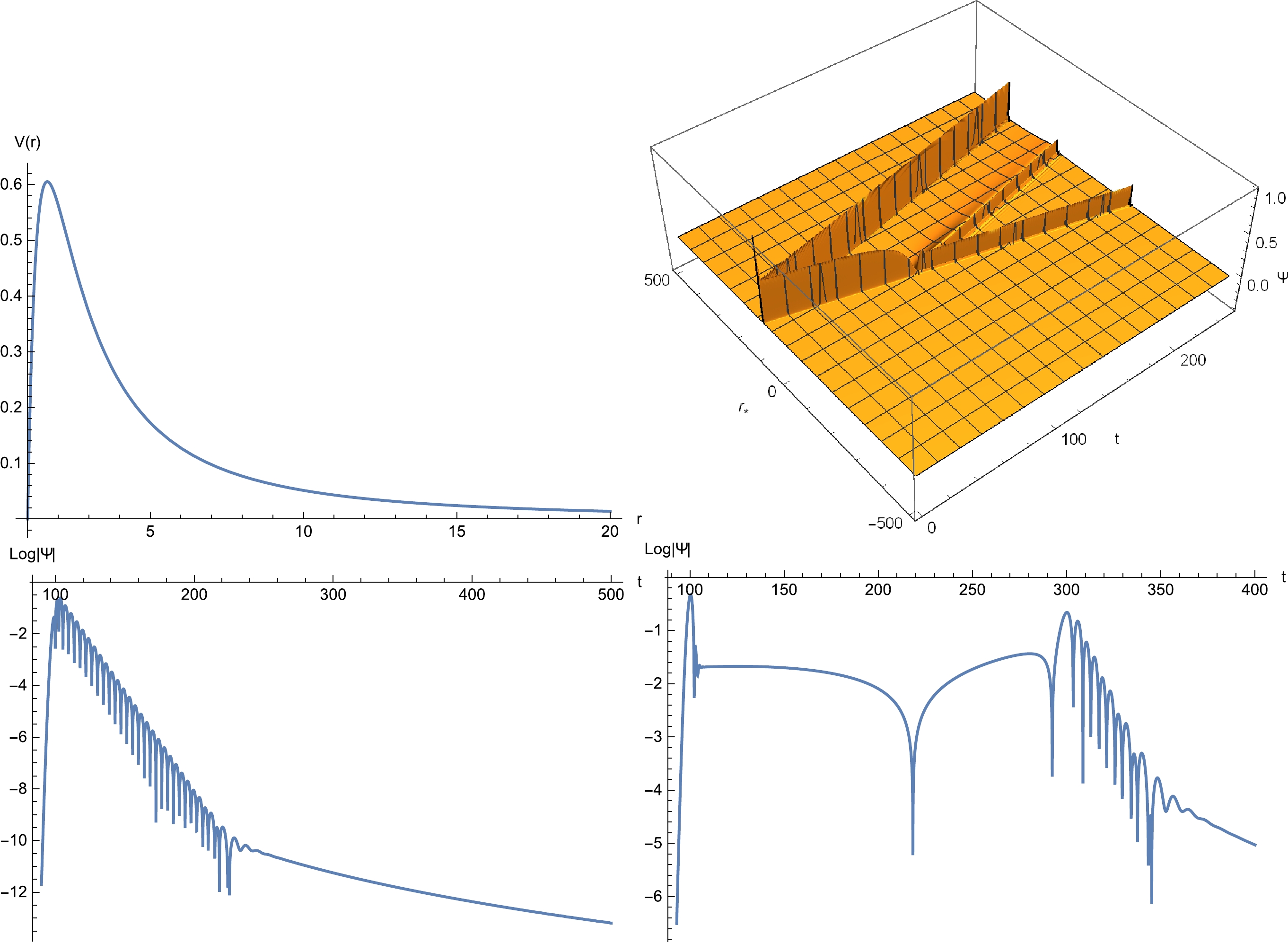

Figure 3.  (color online) Temporal evolution of the axial gravitational perturbations in the Schwarschild black hole with the horizon $ r_p=1 $. Top-left: Effective potential. The maximal value of the potential is located at $ r=1.64039 $ ($ r_*=1.19471 $). Top-right: Two-dimensional profile of the temporal evolution, where the initial conditions read $\Psi(t=0)={\rm e}^{-(r_*-100)^2/2}$ and $ \partial_{t}\Psi(t=0)=0 $, placed outside the maximum potential. Bottom-left: Temporal evolution evaluated at $ r=1.278 $ ($ r_*=0 $), inside the maximum potential. Bottom-right: Temporal evolution evaluated at $ r=194.73 $ ($ r_*=200 $), outside the initial perturbations.

In Fig. 4, the temporal evolutions of the axial gravitational perturbations in a star of uniform density are displayed as the simplest theoretical model for the neutron star. The effective potential is featured by a valley between two maxima located at the center and the maximum of the potential. As a result, the GWs are bounced back and forth in the valley, and subsequently, the echoes are produced in the late stage of dissipative oscillations. Although the observer is located further away from the star, the echoes eventually leak out and appear in the signals.

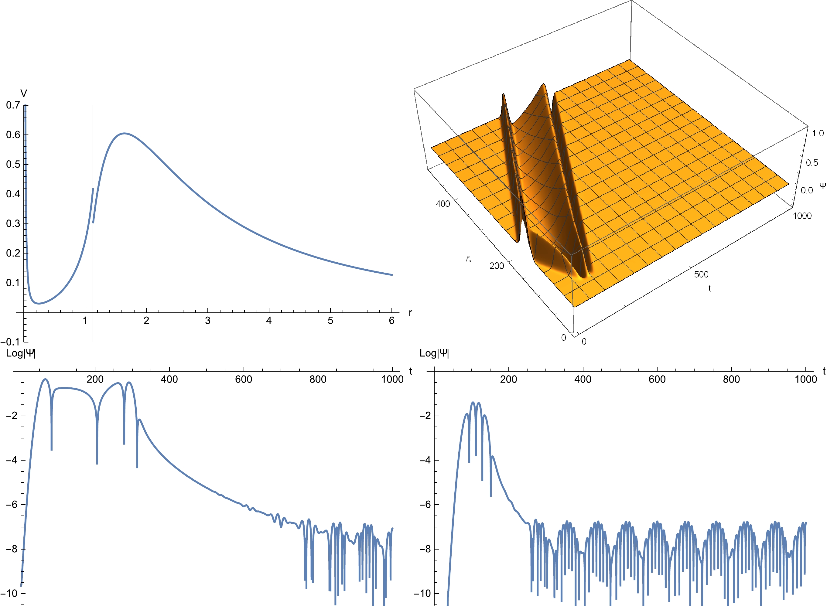
Figure 4.  (color online) Temporal evolution of the axial gravitational perturbations in the star with the surface $ r_b=1.13 $ ($ r_{b*}=36.7 $). Top-left: Effective potential. The maximal value of the potential is located at $ r=1.64039 $ ($ r_*=38.8 $), outside the star's surface. Top-right: Two-dimensional profile of the temporal evolution, where the initial conditions read $\Psi(t=0)={\rm e}^{-(r_*-150)^2/200}$ and $ \partial_{t}\Psi(t=0)=0 $. Due to the scale of the plot, the echoes are not visable in the two-dimensional plot. Bottom-left: Temporal evolution evaluated at $ r=173.937 $ ($ r_*=216.7 $). Bottom-right: Temporal evolution evaluated at $ r=7.256 $ ($ r_*=46.7 $).

For comparison, as shown in Fig. 5, the calculations were similarly conducted with the star's surface placed outside the "original" maximum of the effective potential. However, as shown in the top-left plot, the valley of the effective potential disappears in this case. This is because the matter distribution inside the star dictates that the effective potential decreases monotonically with increasing radial coordinates. Subsequently, no echo is observed in the resultant temporal evolution.

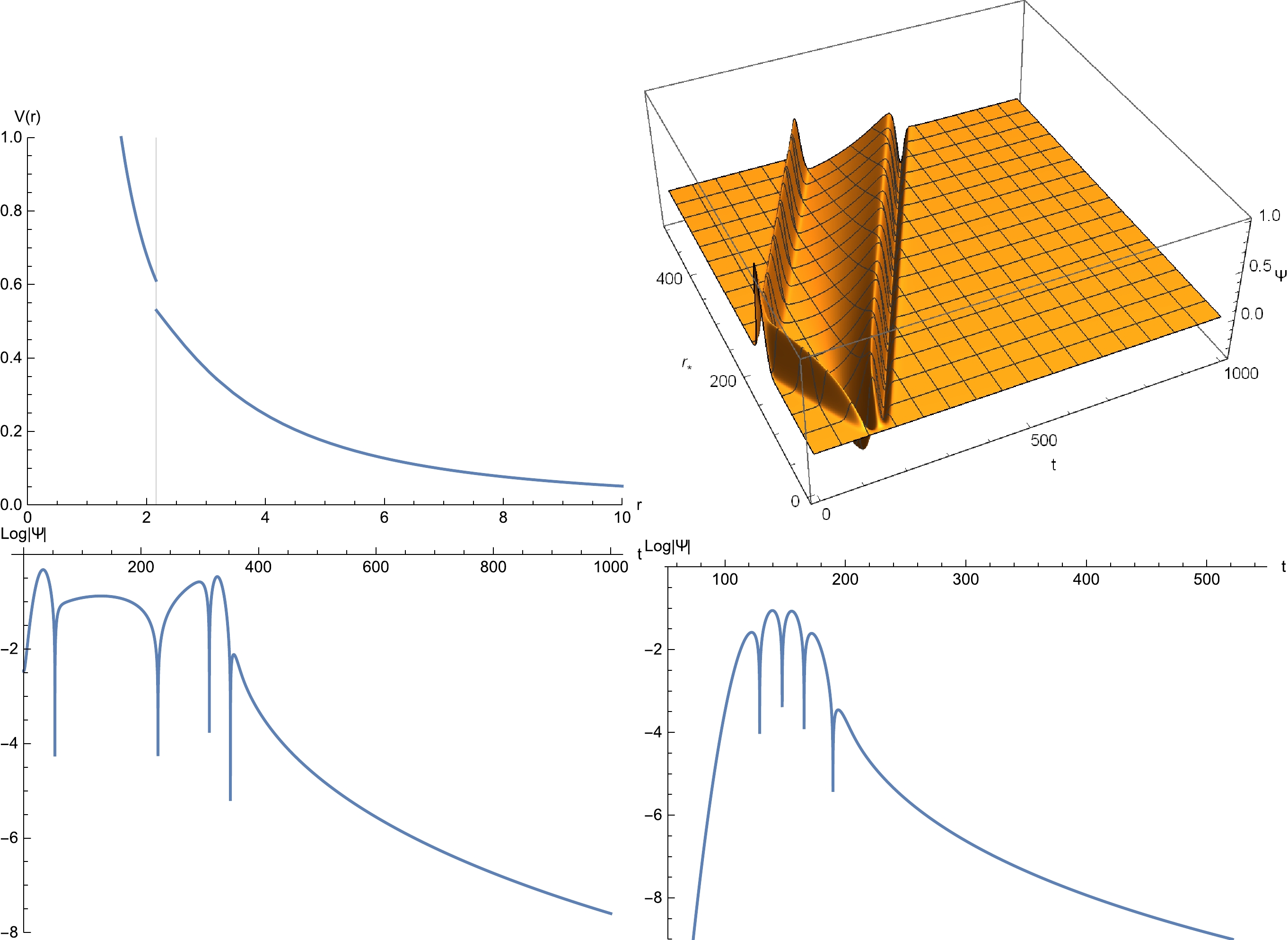
Figure 5.  (color online) The same as Fig. 4 but for $ r_b=2.162 $ ($ r_{b*}=37 $). The bottom-left plot is evaluated at $ r=177.141 $ ($ r_*=183.7 $); the bottom-right plot is evaluated at $ r=10.104 $ ($ r_*=13.7 $).

Using an FDM scheme with appropriate boundary conditions and treatment for the discontinuous boundary, we studied the temporal evolution of axial gravitational perturbations in black holes and uniform stars. The results are shown to be consistent with causality and flow conservation. In particular, echoes are observed in the late-stage of the star QNM oscillations, which is understood to be caused by the valley in the effective potential. Interestingly, the echo period is numerically consistent with twice the distance between the center of the star and the maximum of the effective potential, regardless of the discontinuity at the star's surface [57]. We plan to continue exploring the related topics in the future.