


 Abstract
 HTML
HTML Reference
 Related
 Supplemental material
 PDF
PDF


-
Fast radio bursts (FRBs) are energetic radio pulses with durations on the order of milliseconds happening in the Universe; see, e.g., [1−4] for recent reviews. The discovery of the first FRB dates back to 2007, when Lorimer et al. [5] reanalyzed the 2001 archive data of the Parkes 64-m telescope and found an anomalous radio pulse, which is now named FRB010724. Later, Thornton et al. [6] discovered several other similar radio pulses, and FRBs received great attention within the astronomy community. The origin of FRBs was still a mystery at that time, but the large dispersion measure (DM) implies that they are unlikely to originate from the Milky Way. The identification of the host galaxy and the direct measurement of redshift further confirmed that they have extragalactic origin [7−9]. To date, several hundreds of FRBs have been discovered [10, 11], among which only one is confirmed to originate from our galaxy [12]. FRBs can be divided into two phenomenological types: repeaters and non-repeaters, according to whether they are one-off events or not. The majority of FRBs are apparently non-repeating, but it remains unclear if they will be repeating in the future. Most repeating FRBs are not very active and repeat only two to three times [13]. However, more than one thousand bursts have been observed from two extremely active sources: FRB20121102A [14] and FRB20201124A [15].
The physical origin of FRBs continues to be under extensive debate. Several theoretical models have been proposed to explain repeating and non-repeating FRBs, such as giant pulses from young rapidly rotating pulsars [16], the black hole battery model [17], the "Cosmic Comb" model [18], the inspiral and merger of binary neutron stars [19, 20], neutron star-white dwarf binary model [21], collision between neutron stars and asteroids [22], highly magnetized pulsars travelling through asteroid belts [23, 24], young magnetars with fracturing crusts [25], and axion stars moving through pulsar magnetospheres [26]. Although a standard model has not yet been established, it is widely accepted that the progenitor of an FRB should at least involve one neutron star or magnetar. The recently discovered magnetar-associated burst in our Milky Way strongly supports the magnetar origin of some, if not all FRBs [12, 27]. The statistical similarity between repeating FRBs and soft gamma repeaters further implies that they may have similar origin [28, 29].
FRBs are energetic enough to be detectable up to high redshift; therefore, they can be used as probes to investigate the cosmology [30−37], as well as to test the fundamental physics [38−42]. Unfortunately, up to now, most FRBs have no direct measurement of redshift. Although hundreds of FRBs have been measured, only a dozen of them are well localized. With such a small sample, we even do not clearly know the redshift distribution of FRBs. One way to solve this problem is to use the observed DM, which is an indicator of distance, to infer the redshift [43−46]. Accordingly, the DM contribution from the host galaxy should be reasonably modeled and subtracted from the total observed DM. This is not an easy task because too many factors may affect the host DM, such as the galaxy type, inclination angle, mass of the host galaxy, and offset of FRB site from galaxy center, among others. A simple but approximate assumption is that the host DM is a universal constant for all FRBs [31, 35, 46]. Alternatively, Luo et al. [47] assumed that the host DM follows the star-formation rate (SFR) of the host galaxy. However, Lin et al. [48] found no strong correlation between host DM and SFR from the limited sample of localized FRBs. A more reasonable way to deal with the host DM is to model it using a proper probability distribution and marginalize over the free parameters [36, 49, 50]. For example, Macquart et al. [49] assumed that the host DM follows log-normal distribution, and reconstructed the DM-redshift relation from five well-localized FRBs. However, due to the small data sample, the DM-redshift relation has large uncertainty. With the discovery of more and more FRBs in recent years, it is interesting to recheck the DM-redshift relation and use it to infer the redshift of FRBs, as there is currently no direct measurement of spectroscopic or photometric redshift.
In this paper, we assume that the host DM of FRBs follows log-normal distribution, and reconstruct the DM-redshift relation from well localized FRBs using Bayesian inference. Then, the DM-redshift relation is used to infer the redshift of the first CHIME/FRB catalog [11]. We further consider the inferred redshift to calculate the isotropic energy of the CHIME/FRBs. The rest of this paper is arranged as follows: In section II, we reconstruct the DM-redshift relation from well-localized FRBs. In section III, we investigate the redshift and energy distributions of CHIME/FRBs. Finally, discussion and conclusions are provided in section IV.
-
The interaction of electromagnetic waves with plasma leads to the frequency-dependent light speed. This plasma effect, although small, may cause detectable time delay between electromagnetic waves of different frequencies, if it accumulates at cosmological distance. This phenomenon is more obvious for low-frequency electromagnetic waves, such as the radiowave, as is observed in FRBs, for instance. The time delay between low- and high-frequency electromagnetic waves propagating from a distant source to earth is proportional to the integral of electron number density along the line-of-sight, i.e., the DM. The observed DM of an extragalactic FRB can generally be decomposed into four main parts: Milky Way interstellar medium (
$ {\rm DM_{MW}} $ ), galactic halo ($ {\rm DM_{halo}} $ ), intergalactic medium ($ {\rm DM_{IGM}} $ ), and host galaxy ($ {\rm DM_{host}} $ ) [49, 51, 52],$ \begin{align} {\rm DM_{obs}}={\rm DM_{MW}}+{\rm DM_{halo}}+{\rm DM_{IGM}}+\frac{{\rm DM_{host}}}{1+z}, \end{align} $

(1) where
$ {\rm DM_{host}} $ is the DM of the host galaxy in the FRB source frame, and the factor$ 1+z $ arises from the cosmic expansion. Occasionally, the$ {\rm DM_{halo}} $ term is ignored, but this term is comparable to, or even larger than the$ {\rm DM_{MW}} $ term for FRBs at high Galactic latitude.The Milky Way ISM term (
$ {\rm DM_{MW}} $ ) can be well modeled from pulsar observations, such as the NE2001 model [53] and the YMW16 model [54]. For FRBs at high galactic latitude, both models produce consistent results. However, the YMW16 model may overestimate$ {\rm DM_{MW}} $ at low Galactic latitude [55]. Therefore, we adopt the NE2001 model to estimate$ {\rm DM_{MW}} $ . The galactic halo term ($ {\rm DM_{halo}} $ ) is not well constrained yet, and Prochaska & Zheng [56] estimated that it is approximately$ 50\sim 80\; {\rm pc\; cm^{-3}} $ . Herein, we follow Macquart et al. [49] and assume a conservative estimation, i.e.${\rm DM_{halo}}= 50 {\rm pc\; cm^{-3}}$ . The concrete value of$ {\rm DM_{halo}} $ should not strongly affect our results, as its uncertainty is much smaller than the uncertainties of the$ {\rm DM_{IGM}} $ and$ {\rm DM_{host}} $ terms described bellow. Therefore, the first two terms on the right-hand-side of equation (1) can be subtracted from the observed$ {\rm DM_{obs}} $ . For convenience, we define the extragalactic DM as$ \begin{align} {\rm DM_E}\equiv {\rm DM_{obs}}-{\rm DM_{MW}}-{\rm DM_{halo}}={\rm DM_{IGM}}+\frac{{\rm DM_{host}}}{1+z}. \end{align} $

(2) Given a specific cosmological model, the
$ {\rm DM_{IGM}} $ term can be calculated theoretically. Assuming that both hydrogen and helium are fully ionized [57, 58], the$ {\rm DM_{IGM}} $ term can be written in the standard ΛCDM model as [43, 51]$ \begin{align} \langle{\rm DM_{IGM}}(z)\rangle=\frac{21cH_0\Omega_bf_{\rm IGM}}{64\pi Gm_p}\int_0^z\frac{1+z}{\sqrt{\Omega_m(1+z)^3+\Omega_\Lambda}} {\rm d} z, \end{align} $

(3) where
$ f_{\rm IGM} $ is the fraction of baryon mass in IGM,$ m_p $ is the proton mass,$ H_0 $ is the Hubble constant, G is the Newtonian gravitational constant,$ \Omega_b $ is the normalized baryon matter density,$ \Omega_m $ and$ \Omega_\Lambda $ are the normalized densities of matter (including baryon matter and dark matter) and dark energy, respectively. In this paper, we work in the standard ΛCDM model with the Planck 2018 parameters, i.e.,$ H_0=67.4\; {\rm km\; s^{-1}\; Mpc^{-1}} $ ,$ \Omega_m=0.315 $ ,$ \Omega_\Lambda= $ 0.685, and$ \Omega_{b}=0.0493 $ [59]. The fraction of baryon mass in IGM can be tightly constrained by directly observing the budget of baryons in different states [60], or observing the radio dispersion on gamma-ray bursts [61]. All the observations show that$ f_{\rm IGM} $ is approximately 0.84. Using five well-localized FRBs, Li et al. [33] also obtained the similar result. Therefore, we fix$ f_{\rm IGM}=0.84 $ to reduce the freedom. The uncertainty of these parameters should not significantly affect our results as they are much smaller than the variation of$ {\rm DM_{IGM}} $ described below.Note that equation (3) should be interpreted as the mean contribution from IGM. Due to the large-scale matter density fluctuation, the actual value would vary around the mean. Theoretical analysis and hydrodynamic simulations show that the probability distribution for
$ {\rm DM_{IGM}} $ has a flat tail at large values, which can be fitted with the following function [49, 62]$ \begin{align} p_{\rm IGM}(\Delta)=A\Delta^{-\beta}\exp\left[-\frac{(\Delta^{-\alpha}-C_0)^2}{2\alpha^2\sigma_{\rm IGM}^2}\right], \; \; \; \Delta>0, \end{align} $

(4) where
$ \Delta\equiv{\rm DM_{IGM}}/\langle{\rm DM_{IGM}}\rangle $ ,$ \sigma_{\rm IGM} $ is the effective standard deviation, α and β are related to the inner density profile of gas in haloes, A is a normalization constant, and$ C_0 $ is chosen such that the mean of this distribution is unity. Hydrodynamic simulations indicate that$ \alpha=\beta=3 $ provides the best match to the model [49, 62]; thus, we fix these two parameters. Simulations also show that standard deviation$ \sigma_{\rm IGM} $ approximately scales with redshift as$ z^{-1/2} $ in the redshift range$ z\lesssim 1 $ [63, 64]. The redshift-dependence of$ \sigma_{\rm IGM} $ is still unclear at$ z>1 $ , so we simply extrapolate this relation to high-redshift region. Therefore, following Macquart et al. [49], we parameterize it as$ \sigma_{\rm IGM}=Fz^{-1/2} $ , where F is a free parameter.Due to the lack of detailed observation on the local environment of FRB source, host term
$ {\rm DM_{host}} $ is poorly known and may range from several tens to several hundreds$ {\rm pc\; cm^{-3}} $ . For example, Xu et al. [15] estimated that$ {\rm DM_{host}} $ of repeating burst FRB20201124A is in the range$ 10< {\rm DM_{host}}< 310\; {\rm pc\; cm}^{-3} $ ; Niu et al. [65] inferred$ {\rm DM_{host}}\approx 900\; {\rm pc\; cm}^{-3} $ for FRB20190520B. Numerical simulations show that the probability of$ {\rm DM_{host}} $ follows the log-normal distribution [49, 50],$ \begin{aligned}[b] p_{\rm host}({\rm DM_{host}}|\mu,\sigma_{\rm host})=&\frac{1}{\sqrt{2\pi}{\rm DM_{host}}\sigma_{\rm host}}\\ &\times\exp\left[-\frac{(\ln {\rm DM_{host}}-\mu)^2}{2\sigma_{\rm host}^2}\right], \end{aligned} $

(5) where μ and
$ \sigma_{\rm host} $ are the mean and standard deviation of$ \ln {\rm DM_{host}} $ , respectively. This distribution has a median value of${\rm e}^\mu$ and variance${\rm e}^{\mu+\sigma_{\rm host}^2/2}({\rm e}^{\sigma_{\rm host}^2}-1)^{1/2}$ . Theoretically, the log-normal distribution allows for the appearance of a large value of$ {\rm DM_{host}} $ , as shown by simulations;$ {\rm DM_{host}} $ may be as large as$ 1000\; {\rm pc\; cm}^{-3} $ [44]. Generally, the two parameters ($ \mu,\sigma_{\rm host} $ ) may be redshift-dependent, but for non-repeating bursts, they do not vary significantly with redshift [50]. For simplicity, we first follow Macquart et al. [49] and treat them as two constant parameters. The possible redshift-dependence will be investigated later.Given the distributions
$ p_{\rm IGM} $ and$ p_{\rm host} $ , the probability distribution of$ {\rm DM_E} $ at redshift z can be calculated as [49]$ \begin{aligned}[b] p_E({\rm DM_E}|z)=&\int_0^{(1+z){\rm DM_E}}p_{\rm host}({\rm DM_{host}}|\mu,\sigma_{\rm host})\\ &\times p_{\rm IGM} \left({\rm DM_E}-\frac{\rm DM_{host}}{1+z}|F,z\right){\rm d}{\rm DM_{host}}. \end{aligned} $

(6) The likelihood that we observe a sample of FRBs with
$ {\rm DM_{E,\it i}} $ at redshift$ z_i $ ($ i=1,2,3,...,N $ ) is given by$ \begin{align} {\cal{L}}({\rm FRBs}|F,\mu,\sigma_{\rm host})=\prod_{i=1}^Np_{E}({\rm DM_{E,\it i}}|z_i), \end{align} $

(7) where N is the total number of FRBs. Considering the FRB data (
$ z_i,{\rm DM_{E,\it i}} $ ), the posterior probability distribution of the parameters ($ F,\mu,\sigma_{\rm host} $ ) is obtained according to Bayes theorem by$ \begin{align} P(F,\mu,\sigma_{\rm host}|{\rm FRBs})\propto{\cal{L}}({\rm FRBs}|F,\mu,\sigma_{\rm host})P_0(F,\mu,\sigma_{\rm host}), \end{align} $

(8) where
$ P_0 $ is the prior of the parameters.Thus far, there are 19 well-localized extragalactic FRBs that have direct identification of the host galaxy and well measured redshift
1 . Among them, we ignore FRB20200120E and FRB20190614D: the former is very close to our galaxy (3.6 Mpc) and has a negative redshift of$ z=-0.0001 $ because the peculiar velocity dominates over the Hubble flow [66, 67]. Meanwhile, there is no direct measurement of spectroscopic redshift for the latter, but photometric redshift of$ z\approx 0.6 $ has been determined [68]. The remaining 17 FRBs have well measured spectroscopic redshifts; their main properties are listed inTable 1, which are regarded to reconstruct the$ {\rm DM_E} $ -redshift relation.FRBs RA Dec $ {\rm DM_{obs}} $ 

$ {\rm DM_{MW}} $ 

$ {\rm DM_E} $ 

$ z_{\rm sp} $ 

repeat? reference /( $ ^{\circ} $ )

/( $ ^{\circ} $ )

/( $ {\rm pc cm^{-3}} $ )

/( $ {\rm pc cm^{-3}} $ )

/( $ {\rm pc cm^{-3}} $ )

20121102A $ 82.99 $ 

$ 33.15 $ 

557.00 157.60 349.40 0.1927 Yes Chatterjee et al. [8] 20180301A $ 93.23 $ 

$ 4.67 $ 

536.00 136.53 349.47 0.3305 Yes Bhandari et al. [69] 20180916B $ 29.50 $ 

$ 65.72 $ 

348.80 168.73 130.07 0.0337 Yes Marcote et al. [70] 20180924B $ 326.11 $ 

$ -40.90 $ 

362.16 41.45 270.71 0.3214 No Bannister et al. [71] 20181030A $ 158.60 $ 

$ 73.76 $ 

103.50 40.16 13.34 0.0039 Yes Bhardwaj et al. [72] 20181112A $ 327.35 $ 

$ -52.97 $ 

589.00 41.98 497.02 0.4755 No Prochaska et al. [73] 20190102C $ 322.42 $ 

$ -79.48 $ 

364.55 56.22 258.33 0.2913 No Macquart et al. [49] 20190523A $ 207.06 $ 

$ 72.47 $ 

760.80 36.74 674.06 0.6600 No Ravi et al. [74] 20190608B $ 334.02 $ 

$ -7.90 $ 

340.05 37.81 252.24 0.1178 No Macquart et al. [49] 20190611B $ 320.74 $ 

$ -79.40 $ 

332.63 56.60 226.03 0.3778 No Macquart et al. [49] 20190711A $ 329.42 $ 

$ -80.36 $ 

592.60 55.37 487.23 0.5217 Yes Macquart et al. [49] 20190714A $ 183.98 $ 

$ -13.02 $ 

504.13 38.00 416.13 0.2365 No Heintz et al. [75] 20191001A $ 323.35 $ 

$ -54.75 $ 

507.90 44.22 413.68 0.2340 No Heintz et al. [75] 20191228A $ 344.43 $ 

$ -29.59 $ 

297.50 33.75 213.75 0.2432 No Bhandari et al. [69] 20200430A $ 229.71 $ 

$ 12.38 $ 

380.25 27.35 302.90 0.1608 No Bhandari et al. [69] 20200906A $ 53.50 $ 

$ -14.08 $ 

577.80 36.19 491.61 0.3688 No Bhandari et al. [69] 20201124A $ 77.01 $ 

$ 26.06 $ 

413.52 126.49 237.03 0.0979 Yes Fong et al. [76] Table 1. Properties of the Host/FRB catalog. Column 1: FRB name; Columns 2 and 3: the right ascension and declination of FRB source on the sky, respectively; Column 4: the observed DM; Column 5: the DM of the Milky Way ISM calculated using the NE2001 model; Column 6: the extragalactic DM calculated by subtracting
$ {\rm DM_{\rm MW}} $ and$ {\rm DM_{\rm halo}} $ from the observed$ {\rm DM_{\rm obs}} $ , assuming$ {\rm DM_{\rm halo}}=50\; {\rm pc\; cm^{-3}} $ for the Milky Way halo; Column 7: the spectroscopic redshift; Column 8: indication on whether the FRB is repeating or non-repeating; Column 9: references.We first consider the full 17 FRBs to constrain the free parameters (F,
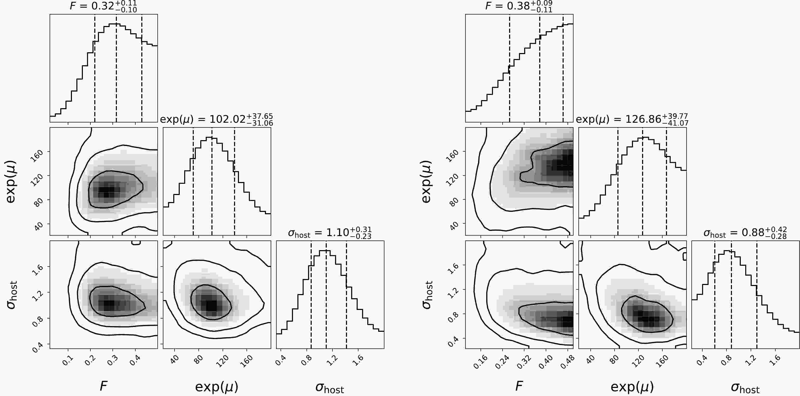
${\rm e}^\mu,\sigma_{\rm host}$ ). We use${\rm e}^\mu$ rather than μ as a free parameter, similar to that used by Macquart et al. [49], because the former directly represents the median value of$ {\rm DM_{host}} $ . The posterior probability density functions of the free parameters are calculated using the publicly available python package$\textsf{emcee} $ [77], while the other cosmological parameters are fixed to the Planck 2018 values [59]. The same flat priors as those used by Macquart et al. [49] are considered for the free parameters:$ F\in {\cal{U}}(0.01,0.5) $ ,$ e^\mu\in {\cal{U}}(20,200)\; {\rm pc\; cm^{-3}} $ , and$ \sigma_{\rm host}\in {\cal{U}}(0.2,2.0) $ . The posterior probability density functions and the confidence contours of the free parameters are plotted in the left panel of Fig. 1. The median values and$ 1\sigma $ uncertainties of the free parameters are$ F=0.32_{-0.10}^{+0.11} $ ,${\rm e}^\mu=102.02_{-31.06}^{+37.65} {\rm pc\; cm^{-3}}$ , and$\sigma_{\rm host}= 1.10_{-0.23}^{+0.31}$ .
Figure 1. Constraints on the free parameters (F,
${\rm e}^\mu, \sigma_{\rm host}$ ) using the full sample (left panel) and the non-repeaters (right panel). The contours from the inner to outer ones represent$ 1\sigma $ ,$ 2\sigma $ , and$ 3\sigma $ confidence regions, respectively.With the parameters (F,
$ e^\mu,\sigma_{\rm host} $ ) constrained, we calculate the probability distribution of$ {\rm DM_E} $ at any redshift in the range$ 0<z<4 $ according to equation (6). The reconstructed$ {\rm DM_E}-z $ relation is plotted in the left panel of Fig. 2. The dark blue line is the median value, and the light blue region is the$ 1\sigma $ uncertainty. For comparison, we also plot the best-fitting curve, obtained by directly fitting equation (2) to the FRB data using the least-$ \chi^2 $ method (the red-dashed line), where$ {\rm DM_{IGM}} $ is replaced by its mean given in equation (3). The least-$ \chi^2 $ method is equivalent to assuming that both$ {\rm DM_{IGM}} $ and$ {\rm DM_{host}} $ follow a Gaussian distribution around the mean. The least-$ \chi^2 $ curve gradually deviates from the median value of the reconstructed$ {\rm DM_E}-z $ relation at high redshift, but due to the large uncertainty, it remains consistent within$ 1\sigma $ uncertainty. We find that 15 out of the 17 FRBs fall well into the$ 1\sigma $ range of the reconstructed$ {\rm DM_E}-z $ relation. Two outliers, FRB20181030A and FRB20190611B (the red dots in Fig. 2), fall bellow the$ 1\sigma $ range of the$ {\rm DM_E}-z $ relation, implying that the$ {\rm DM_E} $ values of these two FRBs are smaller than expected. We note that the outlier FRB20181030A has a much smaller redshift$ (z=0.0039) $ and a very low extragalactic DM ($ {\rm DM_E}=13.34 {\rm pc\; cm^{-3}}) $ ; therefore, the peculiar velocity of its host galaxy cannot be ignored. The redshift of the other outlier FRB20190611B is$ z=0.3778 $ , and the observed DM of this burst is$ {\rm DM_{obs}}=332.63 {\rm pc\; cm^{-3}} $ . The normal burst FRB20200906A has a redshift ($ z=0.3688 $ ) similar to that of FRB20190611B but with a much larger DM ($ {\rm DM_{obs}}=577.8\; {\rm pc\; cm^{-3}} $ ). Note that both FRB20200906A and FRB20190611B are non-repeating, and their positions differ significantly. The large difference in$ {\rm DM_{obs}} $ between these two bursts may be caused by, e.g., the fluctuation of matter density in the IGM, variation of the host DM, or difference in local environment of the FRB source [65, 78].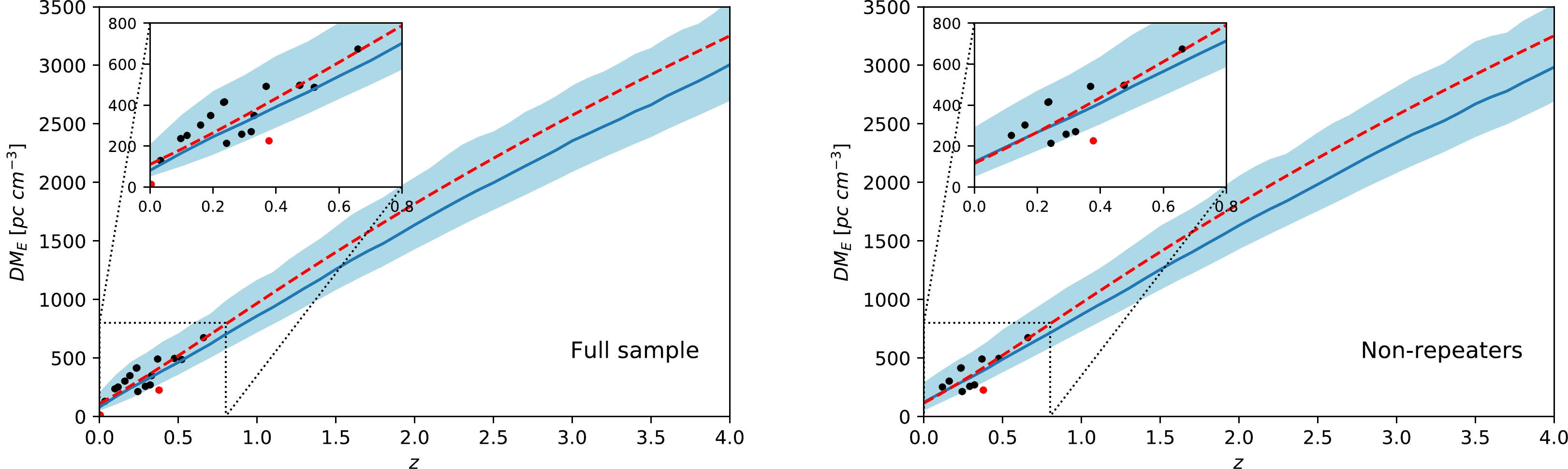
Figure 2. (color online)
$ {\rm DM_E}-z $ relation obtained from full sample (left panel) and non-repeaters (right panel). The dark blue line is the median value, and the light blue region is$ 1\sigma $ uncertainty. The dots are the FRB data points, and the outliers are highlighted in red. The red-dashed line is the best-fitting result obtained using the least-$ \chi^2 $ method. The inset is the zoom-in view of the low-redshift range.The full FRB sample includes 11 non-repeating FRBs and 6 repeating FRBs, which may have different
$ {\rm DM_{host}} $ values. To check this, we re-constrain the parameters ($F,{\rm e}^\mu,\sigma_{\rm host}$ ) using the 11 non-repeating FRBs. The confidence contours and the posterior probability distributions of the parameter space are plotted in the right panel of Fig. 1. The median values and$ 1\sigma $ uncertainties of the free parameters are$ F=0.38_{-0.11}^{+0.09} $ ,${\rm e}^\mu=126.86_{-41.07}^{+39.77} {\rm pc\; cm^{-3}}$ , and$ \sigma_{\rm host}=0.88_{-0.28}^{+0.42} $ . We obtain a slightly larger${\rm e}^\mu$ value but a smaller$ \sigma_{\rm host} $ value than that constrained from the full FRBs. Nevertheless, these values are still consistent with$ 1\sigma $ uncertainty. The reconstructed$ {\rm DM_E}-z $ relation using the non-repeating sample is shown in the right panel of Fig. 2. FRB20190611B is still an outlier (the other outlier FRB20181030A is a repeater). The$ {\rm DM_E}-z $ relations of the full sample and the non-repeaters are well consistent with each other, but the latter has a slightly larger uncertainty, particularly at the low-redshift range.In general,
${\rm e}^\mu$ and$ \sigma_{\rm host} $ may evolve with redshift. Numerical simulations show that the median value of$ {\rm DM_{host}} $ has a power-law dependence on redshift, but$ \sigma_{\rm host} $ does not change significantly [50]. To check this, we parameterize${\rm e}^{\mu}$ in the power-law form,$ \begin{align} {\rm e}^\mu={\rm e}^{\mu_0}(1+z)^\alpha, \end{align} $

(9) and use the full FRB sample to constrain the parameters
$(F, {\rm e}^{\mu_0},\sigma_{\rm host},\alpha)$ . A flat prior is adopted for α in the range$ \alpha\in{\cal{U}}(-2,2) $ . The posterior probability density functions and the confidence contours of the free parameters are plotted in the left panel of Fig. 3. The best-fitting parameters are$ F=0.32_{-0.10}^{+0.11} $ ,${\rm e}^{\mu_0}=98.71_{-33.06}^{+45.75}\; {\rm pc\; cm^{-3}}$ ,$ \sigma_{\rm host} = 1.08_{-0.22}^{+0.32} $ , and$ \alpha=0.15_{-1.33}^{+1.21} $ . As can be seen, parameter α couldn't be tightly constrained, while the constraints on the other three parameters are almost unchanged compared with the case when$ \alpha=0 $ was fixed. This implies that there is no evidence for the redshift-dependence of${\rm e}^\mu$ with the present data. Regarding the non-repeating FRBs, we arrive at the same conclusion (see the right panel of Fig. 3). Therefore, it is safe to assume that${\rm e}^\mu$ is redshift-independent, at least in the low-redshift range$ z<1 $ . However, note that the universality of${\rm e}^\mu$ has not been proven at high redshift. Hence, the uncertainty on the$ {\rm DM_E}-z $ relation in the$ z>1 $ range may be underestimated.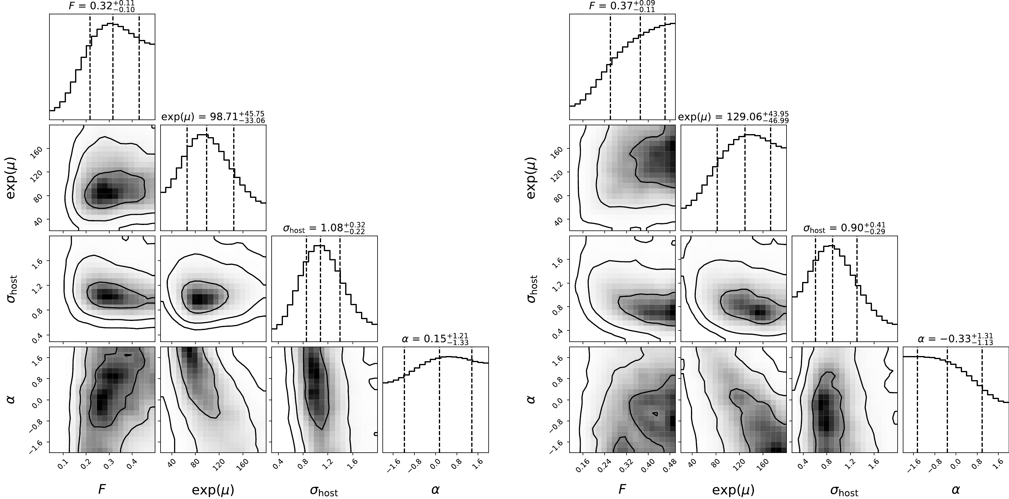
Figure 3. Constraints on the free parameters (
$F, {\rm e}^{\mu_0}, \sigma_{\rm host}, \alpha$ ) using the full sample (left panel) and the non-repeaters (right panel). The contours from the inner to outer ones represent$ 1\sigma $ ,$ 2\sigma $ , and$ 3\sigma $ confidence regions, respectively. -
The first CHIME/FRB catalog comprises 536 bursts, including 474 apparently non-repeating bursts and 62 repeating bursts from 18 FRB sources [11]. In this paper, we focus on the 474 apparently non-repeating bursts, whose properties are listed in a long table in the online material. All the bursts have well measured
$ {\rm DM_{obs}} $ , but there is no direct measurement of their redshift. We calculate the extragalactic$ {\rm DM_E} $ by subtracting$ {\rm DM_{MW}} $ and$ {\rm DM_{halo}} $ from the observed$ {\rm DM_{obs}} $ , where$ {\rm DM_{MW}} $ is calculated using the NE2001 model [53], and$ {\rm DM_{halo}} $ is assumed to be$ 50\; {\rm pc\; cm^{-3}} $ [49]. The$ {\rm DM_E} $ values of the 474 apparently non-repeating bursts fall into the range of$20-3000$ pc cm$ ^{-3} $ . Among them, 444 bursts have$ {\rm DM_E}>100 $ pc cm$ ^{-3} $ , while the remaining 30 bursts have$ {\rm DM_E}<100 $ pc cm$ ^{-3} $ . The mean and median values of$ {\rm DM_E} $ are 557 and 456 pc cm$ ^{-3} $ , respectively. We divide$ {\rm DM_E} $ of the full non-repeating bursts into 30 uniform bins, with bin width$ \Delta{\rm DM_E}=100 $ pc cm$ ^{-3} $ , and plot the histogram in the left panel of Fig. 4. The distribution of$ {\rm DM_E} $ can be well fitted by the cut-off power law (CPL),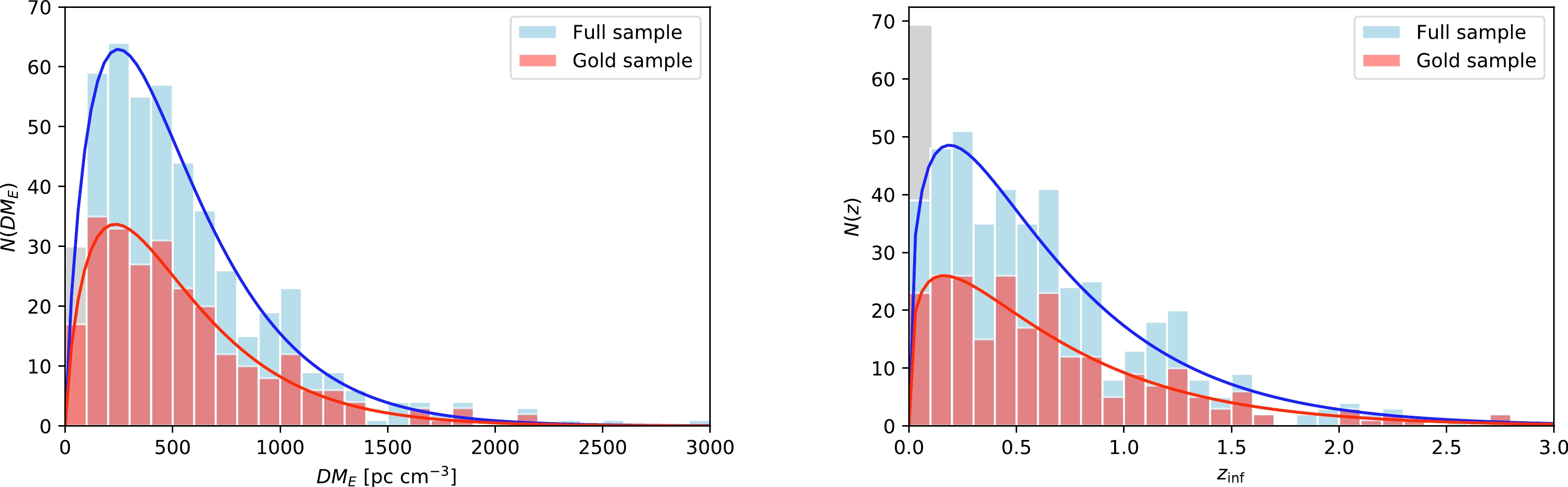
Figure 4. (color online) Histogram of
$ {\rm DM_E} $ (left panel) and inferred redshift (right panel) of the first non-repeating CHIME/FRB catalog. The left-most gray bar represents the 30 FRBs with$ {\rm DM_E}<100\; {\rm pc\; cm^{-3}} $ , which are expected to have$ z<0.1 $ . The blue and red lines are the best-fitting CPL models for the full sample and gold sample, respectively.$ \begin{align} {\rm CPL}:\; \; \; N(x)\propto x^\alpha\exp\left(-\frac{x}{x_c}\right),\; \; \; x>0, \end{align} $

(10) with the best-fitting parameters
$ \alpha=0.86\pm 0.07 $ and$ x_c= 289.49\pm 17.90 $ pc cm$ ^{-3} $ . This distribution exhibits a peak at$ x_p=\alpha x_c\approx 250 $ pc cm$ ^{-3} $ , which is much smaller than the median and mean values of$ {\rm DM_E} $ .Next, we use the
$ {\rm DM_E}-z $ relation reconstructed using the full sample (using the non-repeating sample does not significantly affect our results) to infer the redshift of the non-repeating CHIME/FRBs. For FRBs with$ {\rm DM_E}<100 $ pc cm$ ^{-3} $ , the$ {\rm DM_{host}} $ term may dominate over the$ {\rm DM_{IGM}} $ term, hence a smaller uncertainty on$ {\rm DM_{host}} $ may cause large bias on the estimation of redshift. Therefore, when inferring the redshift using the$ {\rm DM_E}-z $ relation, we only consider the FRBs with$ {\rm DM_E}>100 $ pc cm$ ^{-3} $ . From the$ {\rm DM_E}-z $ relation,$ {\rm DM_E}(z=0.1)= 169.9_{-73.4}^{+196.9} $ pc cm$ ^{-3} $ ($ 1\sigma $ uncertainty). Therefore, FRBs with$ {\rm DM_E}<100 $ pc cm$ ^{-3} $ are expected to have redshift$ z<0.1 $ , while the lower limit cannot be determined. The inferred redshifts for FRBs with$ {\rm DM_E}>100 $ pc cm$ ^{-3} $ are provided in the online material, spanning the range$ z_{\rm inf}\in(0.023,3.935) $ . Three bursts have inferred redshifts larger than 3, i.e., FRB20180906B with$ z_{\rm inf}=3.935_{-0.705}^{+0.463} $ , FRB20181203C with$ z_{\rm inf}=3.003_{-0.657}^{+0.443} $ , and FRB20190430B with$ z_{\rm inf}=3.278_{-0.650}^{+0.449} $ .We divide the redshift range
$ 0<z<3 $ into 30 uniform bins, with bin width$ \Delta z=0.1 $ , and plot the histogram of the inferred redshift in the right panel of Fig. 4. The distribution of the inferred redshift can be fitted via the CPL model given in equation (10). The best-fitting parameters are$ \alpha=0.39\pm 0.09 $ and$ x_c=0.48\pm 0.06 $ . The distribution displays a peak at$ z_p=\alpha x_c\approx 0.19 $ . The mean and median values of this distribution are$ 0.67 $ and$ 0.52 $ , respectively. Considering the FRBs with$ {\rm DM_E}<100 $ $ {\rm pc\; cm}^{-3} $ (30 FRBs in total), which are expected to have$ z<0.1 $ , there is a large excess compared with the CPL model in the redshft range$ z<0.1 $ (see the left-most gray bar in Fig. 4). This may be caused by the selection effect, as the detector is more sensitive to nearer FRBs.Amiri et al. [11] provided a set of criteria to exclude events that are unsuitable for use in population analyses: (1) events with
$ S/N < 12 $ ; (2) events having$ {\rm DM_{obs}} < 1.5{\rm max(DM_{NE2001}, DM_{YMW16})} $ ; (3) events detected in far sidelobes; (4) events detected during non-nominal telescope operations; and (5) highly scattered events ($ \tau_{\rm scat}>10 $ ms). We call the remaining FRBs the gold sample, constituting 253 non-repeating FRBs. We plot the distributions of$ {\rm DM_E} $ and redshifts of the gold sample, together with those of the full sample, in Fig. 4. Similar to the full sample, the distributions of$ {\rm DM_E} $ and redshifts of the gold sample can also be fitted by the CPL model. The best-fitting CPL model parameters are summarized in Table 2. It is clear that the parameters are not significantly changed compared with those of the full sample. Note that the redshift distribution of the gold sample shown in the right panel of Fig. 4 only contains the FRBs with${\rm DM_E > 100 {\rm pc\; cm^{-3}}}$ (236 FRBs). The gold sample still contains 17 FRBs with$ {\rm DM_E<100\; pc\; cm^{-3}} $ , whose redshifts are expected to be$ z<0.1 $ . Thus, the low-redshift excess still exists in the gold sample.$ {\rm DM_E} $ (Full)

$ \alpha=0.86\pm 0.07 $ 

$ x_c=289.49\pm 17.90 {\rm pc cm^{-3}} $ 

$ {\rm DM_E} $ (Gold)

$ \alpha=0.77\pm 0.09 $ 

$ x_c=302.82\pm 23.92 {\rm pc cm^{-3}} $ 

redshift (Full) $ \alpha=0.39\pm 0.09 $ 

$ x_c=0.48\pm 0.06 $ 

redshift (Gold) $ \alpha=0.31\pm 0.11 $ 

$ x_c=0.52\pm 0.08 $ 

Table 2. Best-fitting CPL model parameters for the distributions of
$ {\rm DM_E} $ and redshift.Given the redshift, the isotropic energy of a burst can be calculated as [79]
$ \begin{align} E=\frac{4\pi d_L^2F\Delta\nu}{(1+z)^{2+\alpha}}, \end{align} $

(11) where
$ d_L $ is the luminosity distance, F is the average fluence, α is the spectral index ($ F_\nu\propto \nu^\alpha $ ), and$ \Delta\nu $ is the waveband in which the fluence is observed. The fluence listed in the first CHIME/FRB catalog is averaged over the$ 400-800 $ MHz waveband, hence$ \Delta\nu=400 $ MHz. The spectral indices of some bursts are not clear. Macquart et al. [80] showed that, for a sample of ASKAP/FRBs,$ \alpha=-1.5 $ provides a reasonable fit. Hence, we fix$ \alpha=-1.5 $ for all the bursts. Note that the fluence given in the CHIME/FRB catalog is lower limit, as the fluence is measured assuming each FRB is detected at the location of maximum sensitivity. Therefore, the energy calculated using equation (11) is the lower limit. With the inferred redshift, we calculate the isotropic energy in the standard ΛCDM cosmology with the Planck 2018 parameters [59]. The uncertainty of energy propagates from the uncertainties of fluence and redshift. The results are presented in the online material. The isotropic energy spans approximately five orders of magnitude, from$ 10^{37} $ erg to$ 10^{42} $ erg, with the median value of$ \sim 10^{40} $ erg. Three bursts have energy above$ 10^{42} $ erg, see Table 3. The isotropic energy of the furthest burst, FRB20180906B, is approximately$ 4\times 10^{41} $ erg.FRBs RA Dec $ {\rm DM_{obs}} $ 

$ {\rm DM_{MW}} $ 

$ {\rm DM_E} $ 

Fluence $ z_{\rm inf} $ 

$ \log(E/{\rm erg}) $ 

flag /( $ ^{\circ} $ )

/( $ ^{\circ} $ )

/( $ {\rm pc/cm^{3}} $ )

/( $ {\rm pc/cm^{3}} $ )

/( $ {\rm pc/cm^{3}} $ )

/(Jy ms) 20181219B $ 180.79 $ 

$ 71.55 $ 

$ 1950.7 $ 

$ 35.8 $ 

$ 1864.9 $ 

$ 27.00\pm22.00 $ 

$ 2.300_{-0.511}^{+0.357} $ 

$ 42.405_{-0.962}^{+0.388} $ 

$ 1 $ 

20190228B $ 50.01 $ 

$ 81.94 $ 

$ 1125.8 $ 

$ 81.9 $ 

$ 993.9 $ 

$ 66.00\pm32.00 $ 

$ 1.175_{-0.355}^{+0.205} $ 

$ 42.170_{-0.633}^{+0.324} $ 

$ 0 $ 

20190319A $ 113.43 $ 

$ 5.72 $ 

$ 2041.3 $ 

$ 109.0 $ 

$ 1882.3 $ 

$ 19.40\pm4.20 $ 

$ 2.325_{-0.516}^{+0.359} $ 

$ 42.271_{-0.335}^{+0.214} $ 

$ 1 $ 

Table 3. Most energetic bursts with
$ E>10^{42} $ erg. Column 1: FRB name; Columns 2 and 3: the right ascension and declination of the FRB source on the sky, respectively; Column 4: the observed DM; Column 5: the DM of the Milky Way ISM calculated using the NE2001 model; Column 6: the extragalactic DM calculated by subtracting$ {\rm DM_{\rm MW}} $ and$ {\rm DM_{\rm halo}} $ from the observed$ {\rm DM_{\rm obs}} $ , assuming$ {\rm DM_{\rm halo}}=50\; {\rm pc\; cm^{-3}} $ for the Milky Way halo; Column 7: the observed fluence; Column 8: the inferred redshift; Column 9: the isotropic energy; Column 10: the flag indicating whether the sample is gold (flag=1) or not (flag=0). Note that the uncertainty of energy may be underestimated due to the lack of well-localized FRBs at$ z>1 $ .Several works have shown that the distributions of fluence and energy of repeating FRBs follow a simple power law (SPL) [81, 82]. To check if the fluence and energy of the apparently non-repeating FRBs follow the same distribution, we calculate the cumulative distributions of fluence and energy of the non-repeating CHIME/FRBs (for both the full and gold samples), and plot the results in Fig. 5. We try to fit the cumulative distributions of fluence and energy using the SPL model, where
$ x_c $ is the cut-off value above which the FRB count is zero. The uncertainty of N is given by$ \sigma_N=\sqrt{N} $ [82]. The best-fitting parameters are detailed in Table 4, and the best-fitting lines are shown in Fig. 5 as dashed lines. As can be seen, for both the full sample and the gold sample, the SPL model fails to fit the distributions of fluence and energy. In particular, at the left end, the model prediction considerably exceeds the data points.
Figure 5. (color online) Cumulative distribution of fluence (left panel) and isotropic energy (right panel) of the non-repeating CHIME/FRBs with
$ {\rm DM_E}>100\; {\rm pc\; cm^{-3}} $ . The solid and dashed lines are the best-fitting BPL model and SPL model, respectively.Fluence (full) SPL $ \beta=0.54\pm0.02 $ 

$ x_c=66.30\pm3.52 $ Jy ms

$ \chi^2/{\rm dof}=7.48 $ 

BPL $ \gamma=1.55\pm0.01 $ 

$ x_b=3.36\pm0.04 $ Jy ms

$ \chi^2/{\rm dof}=0.23 $ 

Fluence (gold) SPL $ \beta=0.48\pm0.03 $ 

$ x_c=58.59\pm4.02 $ Jy ms

$ \chi^2/{\rm dof}=5.79 $ 

BPL $ \gamma=1.65\pm0.02 $ 

$ x_b=3.96\pm0.07 $ Jy ms

$ \chi^2/{\rm dof}=0.29 $ 

Energy (full) SPL $ \beta=0.09\pm0.01 $ 

$ x_c=(1.17\pm0.06)\times 10^{42} {\rm erg} $ 

$ \chi^2/{\rm dof}=11.10 $ 

BPL $ \gamma=0.90\pm0.01 $ 

$ x_b=(1.55\pm0.02)\times 10^{40} {\rm erg} $ 

$ \chi^2/{\rm dof}=0.50 $ 

Energy (gold) SPL $ \beta=0.08\pm0.01 $ 

$ x_c=(1.13\pm0.09)\times 10^{42} {\rm erg} $ 

$ \chi^2/{\rm dof}=7.12 $ 

BPL $ \gamma=0.95\pm0.01 $ 

$ x_b=(1.82\pm0.04)\times 10^{40} {\rm erg} $ 

$ \chi^2/{\rm dof}=0.29 $ 

Table 4. Best-fitting parameters of the cumulative distributions of fluence and energy for the full sample and the gold sample.
$ \begin{align} {\rm SPL}:\; \; \; N(>x)\propto(x^{-\beta}-x_c^{-\beta}),\; \; \; x<x_c, \end{align} $

(12) Lin & Sang [83] showed that the bent power law (BPL) model fits the distributions of fluence and energy of repeating burst FRB121102 much better than the SPL model. The BPL model takes the form
$ \begin{align} {\rm BPL}:\; \; \; N(>x)\propto\left[1+\left(\frac{x}{x_b}\right)^\gamma\right]^{-1},\; \; \; x>0, \end{align} $

(13) where
$ x_b $ is the median value of x, i.e.$ N(x>x_b)= N(x<x_b) $ . The BPL model has a flat tail at$ x\ll x_b $ and behaves like the SPL model at$ x\gg x_b $ . The BPL model was initially employed to fit the power density spectra of gamma-ray bursts [84]. Then, it was shown that the BPL model can well fit the distribution of fluence and energy of soft-gamma repeaters [29, 85]. The choice of the BPL model is inspired by the fact that the cumulative distributions of fluence and energy have a flat tail at the left end, as can be seen from Fig. 5. We therefore try to fit the cumulative distributions of fluence and energy of CHIME/FRBs using the BPL model. The best-fitting parameters are summarized in Table 4, and the best-fitting lines are shown in Fig. 5 (solid lines). It is apparent that the BPL model fits the data of both the full and gold samples much better than the SPL model. The BPL model fits the distribution of fluence very well in the full range. For the distribution of energy, the BPL model also fits the data well, except at the very high energy end. -
In this study, we reconstructed the
$ {\rm DM_E}-z $ relation from 17 well-localized FRBs at$ z<1 $ using the Bayesian inference method. The host DM was assumed to follow log-normal distribution with mean$ \exp(\mu) $ and variance$ \sigma_{\rm host} $ , and the variance of the DM of the IGM was assumed to be redshift-dependent ($ \sigma_{\rm IGM}=Fz^{-1/2} $ ). The free parameters were tightly constrained by 17 well-localized FRBs:$ F=0.32_{-0.10}^{+0.11} $ ,$ \exp(\mu)=102.02_{-31.06}^{+37.65}\; {\rm pc\; cm^{-3}} $ , and$\sigma_{\rm host}= 1.10_{-0.23}^{+0.31}$ . These parameters are well consistent with those of Macquart et al. [49], who obtained$ F=0.31_{-0.16}^{+0.13} $ ,$ \exp(\mu)=68.2_{-35.0}^{+59.6}\; {\rm pc\; cm^{-3}} $ , and$\sigma_{\rm host}= 0.88_{-0.45}^{+0.65}$ from five well-localized FRBs. With a larger FRB sample and one less free parameter ($ \Omega_b $ ), our constraint is more stringent than that of Macquart et al. [49]. We directly extrapolated these parameters to high redshift and reconstructed the$ {\rm DM_E}-z $ relation up to$ z=4 $ .We further adopted the
$ {\rm DM_E}-z $ relation to infer the redshift of the first CHIME/FRB catalog. We found that the extragalactic DM of the non-repeating CHIME/FRBs follows a CPL distribution, with a peak at$ 250 $ pc cm$ ^{-3} $ . The inferred redshift of the non-repeating CHIME/FRBs can also be fitted by the CPL distribution but with a significant excess at the low redshift range$ 0<z<0.1 $ , which may be caused by selection effect. Thus, we applied a set of criteria to exclude events that are susceptible to selection effect, as described by Amiri et al. [11]. We found that the extragalactic DM and the redshift of the remaining FRBs (i.e., the gold sample) follow a CPL distribution, and the excess at low redshifts still exists. We further used the inferred redshift to calculate the isotropic energy of the non-repeating CHIME/FRBs. As a result, the distributions of energy and fluence can be well fitted by the BPL model, with power indexes of$ \gamma=0.90\pm 0.01 $ and$ \gamma=1.55\pm 0.01 $ for energy and fluence, respectively. However, the SPL model fails to fit both the distributions of fluence and energy, even for the gold sample. The statistical properties of the non-repeating CHIME/FRBs are similar to those of the bursts from the repeating FRB source, FRB121102 [83]. As the BPL model has a flat tail at the low-energy (low-fluence) end, it detects considerably fewer dim bursts than the SPL model. The flatness at the low-energy (low-fluence) end can be explained by the observational incompleteness, as some dim bursts may be missing from detection. Note that the BPL model reduces to the SPL model at the high energy end,$ N(>E)\propto E^{-\gamma} $ . The power-law index of the energy accumulative distribution is$ \gamma \approx 0.9 $ , corresponding to$ \hat\gamma\approx 1.90 $ for the differential distribution. Interestingly, the power-law index of the non-repeating CHIME/FRBs is similar to that of repeating bursts from the single source FRB 121102, with$ \hat\gamma\approx1.6\sim1.8 $ [82].We emphasize that the CPL distribution of redshift is not intrinsic. The intrinsic redshift distribution should consider the selection effect of the detector. Due to the lack of well-localized FRBs, the intrinsic redshift distribution remains poorly known. Several possibilities have been discussed in literature, such as distributions similar to those of gamma-ray bursts [31], a constant comoving number density with a Gaussian cutoff [86], the SFR history model [43], the modified SFR history model [87], and the compact star merger model with various time delays [43]. In a recent work, Qiang et al. [46] considered several modified SFR history models and found good overall consistency with the observed data of the first CHIME/FRB catalog, as long as the model parameters were chosen properly, but the simple SFR history model was fully ejected by the data. Hackstein et al. [44] investigated three different intrinsic redshift distribution models: the constant comoving density model, SFR history model, and stellar mass density model. After considering the selection effects of the CHIME telescope, they showed that the distribution of the observed redshift should have a CPL shape. The model that fits the CHIME/FRB best remains to be determined in future work. In addition, Shin et al. [88] studied the FRB population assuming a Schechter luminosity function; after calibrating the selection effects, they found that the distribution of redshift exhibits a CPL shape.
When reconstructing the
$ {\rm DM_E}-z $ relation, it is important to reasonably deal with the$ {\rm DM_{host}} $ term. The simplest way is to assume that$ {\rm DM_{host}} $ is a constant [31, 35, 46]. As expected, this is inappropriate because the actual value can vary significantly from burst to burst. Luo et al. [47] parameterized$ {\rm DM_{host}} $ as a function of SFR. However, statistical analysis of the well-localized FRBs showed that there is no strong correlation between$ {\rm DM_{host}} $ and the host galaxy properties, including SFR [48]. Because there is a lack of direct observation on$ {\rm DM_{host}} $ , at present, the most reasonable approach is to model it using a probability distribution. Theoretical analysis and numerical simulations indicate that the probability of$ {\rm DM_{host}} $ can be modeled by a log-normal distribution with mean value μ and deviation$ \sigma_{\rm host} $ [49, 50]. Based on the IllustrisTNG simulation, Zhang et al. [50] showed that$ \exp(\mu) $ has a power-law dependence on redshift, and the power-law indices for repeating and non-repeating FRBs slightly differ. However, we found no evidence for the redshift evolution of$ \exp(\mu) $ here. The median value of$ {\rm DM_{host}} $ for the well localized FRBs obtained herein is approximately$ \exp(\mu)\sim 100\; {\rm pc\; cm^{-3}} $ . This is consistent with$ {\rm DM_{host}} $ of FRB20190608B ($ \sim 137\pm 43\; {\rm pc\; cm^{-3}} $ ) obtained from optical/UV observations [89].Due to the lack of high-redshift FRBs, the uncertainty of the
$ {\rm DM_E}-z $ relation is large at high redshift. The uncertainty mainly comes from those regarding$ {\rm DM_{IGM}} $ and$ {\rm DM_{host}} $ . The uncertainty on$ {\rm DM_{IGM}} $ at redshift$ z=1 $ is approximately$ \delta{\rm DM_{IGM}}\approx 0.3{\rm DM_{IGM}}\approx 270\; {\rm pc\; cm^{-3}} $ . From the lognormal distribution, the uncertainty of$ {\rm DM_{host}} $ is estimated to be$\delta {\rm DM_{host}}=\exp(\mu+\sigma_{\rm host}/2) \times (\exp(\sigma_{\rm host}^2)- 1)^{1/2} \approx 200\; {\rm pc\; cm^{-3}}$ , where$\exp(\mu)\approx 100 {\rm pc\; cm^{-3}}$ and$ \sigma_{\rm host}\approx 1 $ . The uncertainties of$ {\rm DM_{MW}} $ and$ {\rm DM_{halo}} $ are expected to be much smaller than those of$ {\rm DM_{IGM}} $ and$ {\rm DM_{host}} $ and were thus ignored herein. We also ignored the DM of the FRB source, which is difficult to model due to the lack of knowledge on the local environment of FRBs. With the present knowledge, the probability distribution of$ {\rm DM_{source}} $ remains unclear. In some models involving the merger of compact binary, this term is expected to be small [90, 91]. Therefore, in most studies, this term is directly neglected. If$ {\rm DM_{source}} $ does not strongly vary from burst to burst (such that it can be treated approximately as a constant), it can be absorbed into the$ {\rm DM_{host}} $ term, while the probability distribution$ p_{\rm host} $ does not change except for an overall shift. In this case, parameter$ \exp(\mu) $ should be explained as the median value of the sum of$ {\rm DM_{host}} $ and$ {\rm DM_{source}} $ . Therefore, if$ {\rm DM_{source}} $ does not vary significantly, its inclusion should not affect our results. Another uncertainty comes from parameter$ f_{\rm IGM} $ . In general,$ f_{\rm IGM} $ should be treated as a free parameter, together with F,$ \exp(\mu) $ , and$ \sigma_{\rm host} $ . However, due to the small FRB sample, free$ f_{\rm IGM} $ will lead to an unreasonable result. Therefore, we fixed$ f_{\rm IGM}= $ 0.84 based on other independent observations. This will lead to underestimation of the uncertainty of the$ {\rm DM_E}-z $ relation.The conclusions of our paper are based on the assumption that the
$ {\rm DM}_E-z $ relation obtained from low-redshift data can be extrapolated to a high redshift region. As demonstrated in section II, there is no strong evidence for the redshift dependence of the host DM, at least in the low-redshift region$ z\lesssim 1 $ . However, we cannot prove this assumption at the high redshift region because there is a lack of data points at$ z>1 $ . Therefore, we simply extrapolated the$ {\rm DM}_E-z $ relation to the high redshift region without proving it. Recent works [79, 87] have shown that the$ {\rm DM}_E-z $ relation may be nonmonotonic, with a turn point at a certain redshift. This is because an FRB at a low redshift is easier to detect than one at a high redshift, for a given intrinsic luminosity. Therefore, a highly dispersed FRB is mainly caused by a large DM of the host galaxy, rather than by a high redshift. For example, the large DM of FRB20190520B ($ {\rm DM_{obs}}\approx 1200 {\rm pc\; cm}^{-3} $ ,$ z\approx 0.241 $ ) is mainly attributed to the large value of$ {\rm DM_{host}} $ ($ \approx 900\; {\rm pc\; cm}^{-3} $ ) [65]. Therefore, the uncertainty of the$ {\rm DM}_E-z $ relation obtained in this study may be significantly underestimated. We hope that the uncertainty can be reduced if more high-redshift FRBs are detected in the future. -
The parameters of the first (non-repeating) CHIME/ FRB catalog are listed in a long table in the online material.
Inferring redshift and energy distributions of fast radio bursts from the first CHIME/FRB catalog
- Received Date: 2023-03-10
- Available Online: 2023-08-15
Abstract: We reconstruct the extragalactic dispersion measure – redshift (


 DownLoad: