


 Abstract
 HTML
HTML Reference
 Related
 Supplemental material
 PDF
PDF


-
Nuclear charge radius is one of the fundamental properties of an atomic nucleus and is important in studying the evolution of nuclear structures such as halos and shape transition and coexistence [1−10]. Experimentally, nuclear charge radii can be measured at relatively high precision using various methods, including high energy elastic electron scattering [11, 12],
$ K_{\alpha} $ X-ray isotope shifts [13−15], and high-resolution laser spectroscopy [9, 16]. The latest CR2013 experimental database contains 956 root-mean-squared nuclear charge radii of 92 elements from$ ^1 $ H to$ ^{96} $ Cm [17, 18].Theoretically, nuclear charge radii can be calculated using several empirical formulas [19−28], the simplest of which is
$ 1.2 A^{1/3} $ fm [29] (where A is the mass number). There are also many microscopic models [30−38], macroscopic-microscopic approaches [39−43], and local or regional methods [44−47] that have been developed to describe and predict nuclear charge radii. For example, the root-mean-squared deviation (RMSD) in describing nuclear charge radii is approximately 0.027 fm for the Skyrme-Hartree-Fock-Bogoliubov (SHFB) model [33], 0.035 fm for the finite-range liquid-drop model (FRLDM) [41], and 0.01 fm for the Garvey-Kelson relations (GK) [44]. In addition, machine learning is also widely used to study nuclear charge radii [48−52].Recently, two types of methods have been proved to have very high precision in describing and predicting nuclear charge radii. The first is local relations consisting of the charge radii of four neighboring nuclei, denoted by
$\delta R_{i {n} - j {p}}$ ($ i, j = 1, 2 $ ) [53, 54]. The descriptive RMSD of$\delta R_{1n - 1p}$ is only 0.0072 fm for 650 nuclei with both neutron and proton numbers larger than 8 [54]. The accuracy can be further improved if four abnormal regions are excluded, as mentioned in Ref. [46]. The second is the relations of the charge-radius difference of two isotopes, denoted by$ \delta R_k $ (where$ k \geq 1 $ is an integer), and the RMSD for the case of$ k=1 $ is 0.0050 fm for 651 nuclei with the neutron number larger than 20 and three abnormal regions excluded [55].This study improves upon the above two types of relations, and this paper is organized as follows: In Sec. II, we improve
$ \delta R_k $ by considering a term depending on the proton number and the parity of the neutron number and combine the improved$ \delta R_k $ with the$\delta R_{i {n} - j {p}}$ relations. In Sec. III, we investigate the predictive power of our improved relations and predict some unknown nuclear charge radii. Finally, we conclude this paper in Sec. IV. -
Let us begin with
$ \delta R_{k} (N,Z) $ [55], which is defined as$ \delta R_k (N,Z) = R(N,Z) - R(N-k,Z) = \sum\limits^{k-1}_{l = 0} \delta R_1 (N-l,Z) \; , $

(1) where
$ R(N,Z) $ is the root-mean-squared charge radius of a nucleus with neutron number N and proton number Z.The empirical formula for
$ \delta R_1 (N,Z) $ given by Ref. [55] is$ \begin{aligned}[b] & \delta R^{\rm emp}_1 (N,Z) = a (N - N_0) + b \; , \\ & a = \begin{cases} a_{1}, \; N < N_{0} \\ a_{2}, \; N \geq N_{0} \end{cases}\; \end{aligned} $

(2) for
$ N > 20 $ , where$ a_1 $ ,$ a_2 $ , and b are optimized parameters, and$ N_0 $ equals 24, 39, 66, 109, and 155 for N in the ranges$ 21 \sim 28 $ ,$ 29 \sim 50 $ ,$ 51 \sim 82 $ ,$ 83 \sim 126 $ , and above 127, respectively. For the case of$ k>1 $ ,$ \delta R^{\rm emp}_k (N,Z) $ is calculated using Eqs. (1)−(2) [55]. Here, nuclei in three abnormal regions should be excluded in the calculation: (1)$ N = 60 $ and$ 37 \leq Z \leq 41 $ ; (2)$ 88 \leq N \leq 90 $ and$ 62 \leq Z \leq 67 $ ; (3)$ N \leq 106 $ and$ Z = 80 $ , or$ N \leq 108 $ and$ Z = 78 $ or 79 [55].In Fig. 1 (a), we plot the deviations between the experimental values of
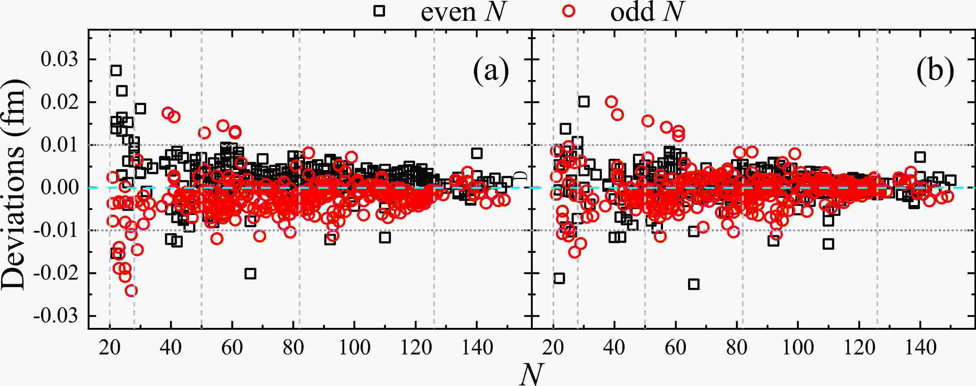
$ \delta R_1 $ (denoted by$ \delta R^{\rm exp}_1 $ ) and$ \delta R^{\rm emp}_1 (N,Z) $ calculated using Eq. (2) versus the neutron number N, where the black squares and red circles correspond to even N and odd N, respectively. We can see that the deviations are different for the parity of N.
Figure 1. (color online) Panel (a) is
$\delta R^{\rm exp}_1 - \delta R^{\rm emp}_1$ versus N, and panel (b) is$\delta R^{\rm exp}_1 - \delta R^{\rm emp1}_1$ versus N. The black squares and red circles correspond to even N and odd N, respectively. The gray dashed lines mark the magic numbers of the neutron. The cyan dashed and purple dotted lines are used to guide the eye.To reduce the odd-even effect, we consider a Z-dependent correction term and rewrite Eq. (2) as
$ \begin{array}{*{20}{l}} \delta R^{\rm emp1}_1 (N,Z) = a ( N - N_0) + b + c |Z-Z_0| \; , \end{array} $

(3) where c equals
$ c_1 $ or$ c_2 $ for even N or odd N, and$ Z_0 $ is the proton number at the half-filled proton shell. The parameters for different neutron shells are given in Table 1, obtained by fitting the experimental values of the nuclear charge radii compiled in the CR2013 database [18]. As shown in Fig. 1 (b), the difference for the parity of N is reduced in the case of$ \delta R^{\rm exp}_1 - \delta R^{\rm emp1}_1 $ .$a_1$ 

$a_2$ 

b $c_1$ 

$c_2$ 

$21 \leq N \leq 28$ 

$-$ 2.475

$-$ 2.559

$-$ 9.165

4.243 $-$ 0.080

$29 \leq N \leq 50$ 

$-$ 1.740

$-$ 0.721

1.586 1.018 0.346 $51 \leq N \leq 82$ 

$-$ 0.802

$-$ 0.346

7.016 0.092 $-$ 0.381

$83 \leq N \leq 126$ 

$-$ 0.459

0.117 2.339 0.175 $-$ 0.092

$N \geq 127$ 

$-$ 0.044

– 4.822 0.235 0.195 Table 1. Optimized parameters
$a_{1}, a_{2}, b, c_1$ , and$c_2$ (in units of$10^{-3}$ fm) in Eq. (3) for different neutron shells, based on the CR2013 database [18].The RMSD (denoted by σ) of
$ \delta R_k $ is defined as$ \sigma = \left\{ \frac{1}{\mathbb{N}} \left[ D (N,Z) \right]^2 \right\}^{1/2} \; , $

(4) where
$ D (N,Z) $ is the deviation between the experimental and theoretical values of$ \delta R_k $ , and$ \mathbb{N} $ is the total number of$ D (N,Z) $ under consideration. According to Eq. (4), σ of Eq. (3) is 0.0041 fm for 651 nuclear charge radii, which is more accurate by approximately 18% compared with that of Eq. (2). -
The
$\delta R_{i { n} - j { p}}$ ($ i,j = 1,2 $ ), proposed based on the independent particle shell model, is defined as [53, 54]$ \begin{aligned}[b] \delta R_{i { n} - j { p}} (N,Z) = & R(N,Z) + R(N-i,Z-j) \\ & -R(N-i,Z) - R(N,Z-j) \approx 0 \; . \end{aligned} $

(5) By substituting Eq. (1) into Eq. (5), we have
$ \begin{aligned}[b] \delta R_{i { n} - j { p}} (N,Z) = & R(N,Z) - R(N-i,Z) \\ & - \delta R_i (N,Z-j) \approx 0 \; . \end{aligned} $

(6) Here,
$ \delta R_i $ can be calculated using Eq. (1), with$ \delta R_1 $ given by Eq. (2) or Eq. (3), and the corresponding calculated$\delta R_{i { n} - j { p}}$ is denoted by$\delta R_{i { n} - j { p}}^{\rm emp}$ or$\delta R_{i n - j { p}}^{\rm emp1}$ . Note that the value of$\delta R_{i { n} - j { p}}^{\rm emp}$ is independent of j because$ \delta R_1 $ given by Eq. (2) is independent of Z.We label the equation
$\delta R_{i { n} - j { p}} = 0$ with$ i = j = 1 $ ,$ i = 1 $ and$ j = 2 $ ,$ i = 2 $ and$ j = 1 $ ,$ i = j = 2 $ as$ E_1 $ ,$ E_2 $ ,$ E_3 $ ,$ E_4 $ , respectively. According to Eq. (6), if the value of$ R(N,Z) $ or$ R(N-i,Z) $ is known, we can calculate the value of the other. Thus, there are up to two possible approaches for each equation to evaluate R of a given nucleus. This leads to the RMSD of the averaged R (denoted by$ \overline{\sigma} $ ), which is defined as$ \overline{\sigma} = \left[ \frac{1}{\mathcal{N}} \sum\limits_{l=1}^{\mathcal{N}} \left( R_l^{\rm exp} - \overline{R}_l^{\rm th} \right)^2 \right]^{1/2} \; ,$

(7) where
$ \mathcal{N} $ is the total number of nuclei under consideration,$ \overline{R}_l^{\rm th} $ is the averaged value of all available calculated results for the l-th nucleus, and$ R_l^{\rm exp} $ is the corresponding experimental value.Based on the CR2013 database [18],
$ \overline{\sigma} $ calculated using Eq. (7) for different combinations of$ E_1 \sim E_4 $ and the corresponding$ \mathcal{N} $ are listed in Table 2, for the cases$R_{i {n} - j {p}}$ ,$R^{\rm emp}_{i {n} - j {p}}$ , and$R^{\rm emp1}_{i {n} - j {p}}$ . Here,$ A_q $ ($ q = 1, 2, 3, 4 $ ) in rows$ 2 \sim 5 $ and$ B_q $ ($ q = 1, 2 $ ) in rows$ 6 \sim 7 $ correspond to combinations of two and three equations taken from$ E_1 \sim E_4 $ , respectively, that is,$ \overline{R}_l^{\rm th} $ in Eq. (7) is the averaged value of up to four and six possible approaches. The results for the combination of all four equations$ E_1 \sim E_4 $ are listed in the last row (labeled as "Total"). The last four columns correspond to the results of the same nuclei that can be calculated by$ A_q $ or$ B_q $ and "Total." The results of$ B_q $ and "Total" are invalid for$\delta R_{i { n} - j { p}}^{\rm emp}$ because of the independence of j, as mentioned above, that is, the value of i should be different for the equations in one combination. As shown in Table 2, the RMSDs of$\delta R_{i { n} - j { p}}^{\rm emp1}$ and$\delta R_{i { n} - j { p}}^{\rm emp}$ are smaller than those of$\delta R_{i { n} - j { p}}$ by$4\% \sim 39\%$ . The optimized combinations are$ A_1 $ ,$ A_3 $ , and$ B_1 $ , with the RMSDs of$\delta R_{i { n} - j { p}}^{\rm emp1}$ as small as that of$ \delta R^{\rm emp1}_1 $ [see Eq. (3)], while the relatively larger RMSDs of$ A_2 $ ,$ A_4 $ ,$ B_2 $ , and "Total" may be caused by equation$ E_4 $ .$\mathcal{N}$ 

$\delta R_{i { n} - j { p} }$ 

$\delta R_{i { n} - j { p} }^{\rm emp}$ 

$\delta R_{i { n} - j { p} }^{\rm emp1}$ 

$\mathcal{N}$ 

$\delta R_{i { n} - j { p} }$ 

$\delta R_{i { n} - j { p} }^{\rm emp}$ 

$\delta R_{i { n} - j { p} }^{\rm emp1}$ 

$A_{1}$ 

688 0.0055 0.0044 0.0043 548 0.0056 0.0045 0.0045 $A_{2}$ 

773 0.0057 0.0054 0.0053 0.0051 0.0049 0.0049 $A_{3}$ 

739 0.0073 0.0046 0.0045 0.0055 0.0047 0.0046 $A_{4}$ 

649 0.0065 0.0058 0.0057 0.0059 0.0051 0.0051 $B_{1}$ 

750 0.0071 – 0.0043 736 0.0071 – 0.0043 $B_{2}$ 

778 0.0061 – 0.0050 0.0058 – 0.0045 Total 792 0.0060 – 0.0051 0.0056 – 0.0046 Table 2. RMSDs (in fm) for different combinations of
$E_1 \sim E_4$ , based on the CR2013 database [18], for the cases$R_{i {n} - j {p}}$ ,$R^{\rm emp}_{i {n} - j {p}}$ , and$R^{\rm emp1}_{i {n} - j {p}}$ . The corresponding number$\mathcal{N}$ of nuclei that can be calculated is also listed.$A_q$ ($q = 1, 2, 3, 4$ ) in rows$2 \sim 5$ [$B_q$ ($q = 1, 2$ ) in rows$6 \sim 7$ ] correspond to combinations of two (three) equations.$A_1$ :$E_1$ and$E_3$ ;$A_2$ :$E_1$ and$E_4$ ;$A_3$ :$E_2$ and$E_3$ ;$A_4$ :$E_2$ and$E_4$ ;$B_1$ :$E_1$ ,$E_2$ and$E_3$ ;$B_2$ :$E_1$ ,$E_2$ and$E_4$ . "Total" in the last row corresponds to the results for the combination of all four equations$E_1 \sim E_4$ . The last four columns are the results of the same nuclei that can be calculated by$A_q$ or$B_q$ and "Total."Because of the high accuracy of these combinations, the deviations between the experimental and our theoretical values of charge radii should be small. However, there are some exceptions. For example, deviations
$ R^{\rm exp} - \overline{R}^{\rm th} $ of several isotopes versus N in three different regions are given in Fig. 2 (d), (e), and (f), where$ \overline{R}^{\rm th} $ is calculated using combination$ B_1 $ of$\delta R_{i { n} - j { p}}^{\rm emp1}$ . The deviations around$ N = 60 $ , 89, and 107 (labeled by gray dashed lines) are relatively larger than the others, which is consistent with the anomalies of the$\delta R_{ nn}$ relation and the linear dependence of R in terms of the valence nucleon numbers, as discussed in Refs. [10, 46]. The anomalies in Fig. 2 (d) and (e) correspond to the sudden increase in R, as shown in Fig. 2 (a) and (b), which is related to the phase transition at$ N = 60 $ ,$ Z \sim 40 $ and the$ Z = 64 $ subshell [56]; the anomalies in Fig. 2 (f) correspond to the sudden decrease in and obvious odd-even staggering of R, as shown in Fig. 2 (c), which belong to a complex region where deformations, transitions, and shape coexistence exist [57, 58]. This shows that the evolution of nuclear structures can be reflected from these combinations.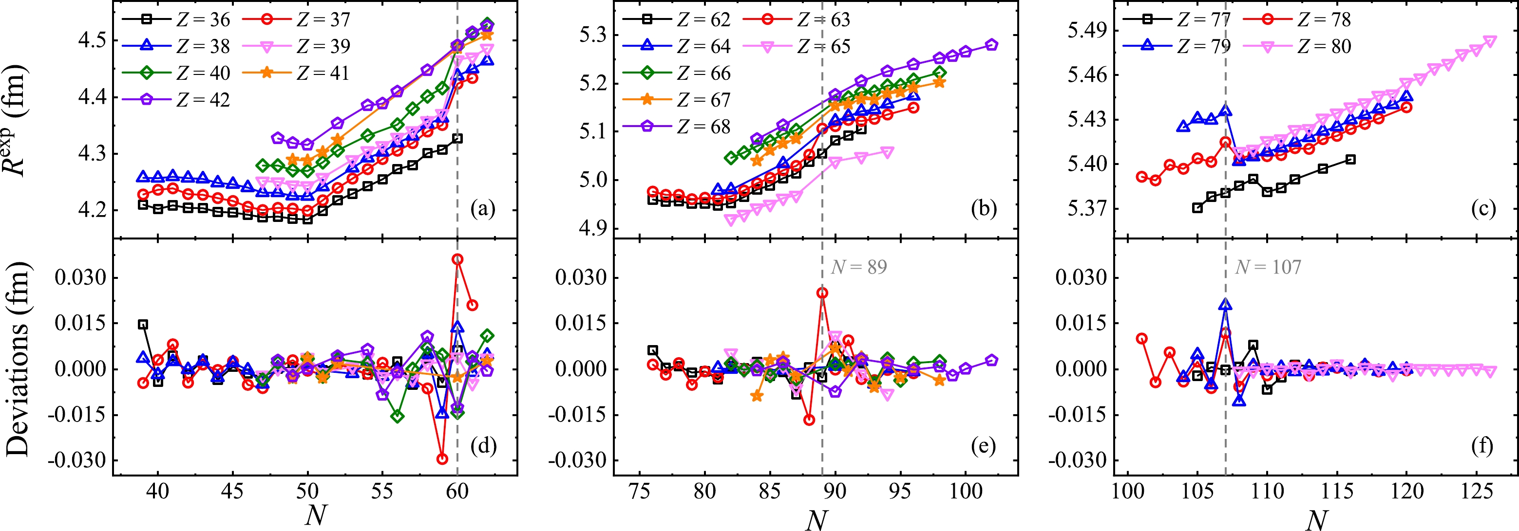
Figure 2. (color online) Panels (a), (b), and (c) show the charge radii of several isotopes versus N in different regions, and panels (d), (e), and (f) show the corresponding deviations
$R^{\rm exp} - \overline{R}^{\rm th}$ , where$\overline{R}^{\rm th}$ is calculated using combination$B_1$ of$\delta R_{i { n} - j { p}}^{\rm emp1}$ . The gray dashed lines are used to guide the eye. -
In this section, we investigate the predictive power of our improved
$ \delta R_k $ relations as well as combinations of$ \delta R_{k} $ and$\delta R_{i { n} - j { p}}$ , that is,$ A_1 $ ,$ A_3 $ , and$ B_1 $ , as mentioned in Sec. II.B. Here, we consider two extrapolations. The first is from the CR1999 database with 239 experimental nuclear charge radii [59] to the CR2013 database [18], with the RMSD calculated using Eq. (7), denoted by$ \sigma_{\rm ex1} $ . The second is from the CR2004 database with 692 experimental values [60] to the CR2013 database [18], with the RMSD denoted by$ \sigma_{\rm ex2} $ . It should be noted that the experimental values in the CR1999 and CR2004 databases are replaced with those in the CR2013 database in both of these extrapolations. -
According to Eq. (1), we have
$ \begin{aligned}[b] R^{\rm pred}_k (N,Z) = & R (N-k,Z) + \delta R^{\rm th}_k (N,Z), \\ R^{\rm pred}_k (N,Z) = & R (N+k,Z) - \delta R^{\rm th}_k (N+k,Z), \end{aligned} $

(8) where
$ R^{\rm pred}_k $ is our predicted charge radius, and$ \delta R^{\rm th}_k $ can be calculated using Eq. (1) with$ k = 1 \sim 15 $ and$ \delta R_1 $ given by Eq. (2) or Eq. (3); it can also be calculated using other theoretical databases, as discussed in Ref. [55], the most accurate of which is the WS* model [22]. The theoretical uncertainties of$ R^{\rm pred}_k $ are calculated following the method in Ref. [55]. As in Ref. [55], there are up to 30 predictions for a given nucleus on the basis of Eq. (8), and the value with the smallest theoretical uncertainty is taken as our predicted charge radius, that is,$ \overline{R}_l^{\rm th} $ in Eq. (7).Table 3 lists
$ \sigma_{\rm ex1} $ and$ \sigma_{\rm ex2} $ for the same nuclei that can be predicted using Eq. (8) with$ \delta R^{\rm th}_k $ calculated based on the WS* model [22], Eq. (2) [55], and Eq. (3). The corresponding number$ \mathcal{N} $ of nuclei that can be predicted is also listed in parentheses in the first column. Obviously, both$ \sigma_{\rm ex1} $ and$ \sigma_{\rm ex2} $ for Eq. (3) are smaller than those for Eq. (2). On account of the$ N = 40 $ subshell effect,$ \sigma_{\rm ex2} $ of Eq. (2) should decrease to 0.0129 fm with Ga isotopes excluded, as discussed in Ref. [55], while the$ N = 40 $ subshell has no significant effect on$ \sigma_{\rm ex2} $ of Eq. (3), which equals 0.0124 fm with Ga isotopes included and is even smaller than that of Eq. (2) with Ga isotopes excluded. Similar to Ref. [55], the average value of the results obtained using Eq. (3) and the WS* model [22] is taken as the theoretical prediction$ R^{\rm pre} $ of a given nucleus, and the corresponding theoretical uncertainty$ \sigma^{\rm pre} $ is also calculated following the method in Ref. [55].WS* Eq. (2) Eq.(3) $\sigma_{\rm ex1} (464)$ 

0.0133 0.0125 0.0110 $\sigma_{\rm ex2} (133)$ 

0.0121 0.0148 0.0124 -
According to Eq. (6), if the value of
$ R(N,Z) $ or$ R(N-i,Z) $ is known, we can predict the other with$ \delta R_i (N,Z-j) $ calculated using Eq. (1) and$ \delta R_1 $ given by Eq. (2) or Eq. (3). For the$ A_{1} $ or$ A_{3} $ ($ B_{1} $ ) combination, there are up to four (six) predictions of a given nucleus, and the averaged value is taken as our predicted charge radius.$ \sigma_{\rm ex1} $ and$ \sigma_{\rm ex2} $ of combinations$ A_{1} $ ,$ A_{3} $ , and$ B_{1} $ for the cases$\delta R_{i { n} - j { p}}$ ,$\delta R_{i { n} - j { p}}^{\rm emp}$ , and$\delta R_{i { n} - j { p}}^{\rm emp1}$ , as well as the corresponding number of nuclei that can be predicted, are given in Table 4. Here, only nuclei that can be predicted by all three relations are considered.$\sigma_{\rm ex1}$ 

$\sigma_{\rm ex2}$ 

$A_1$ (364)

$A_3$ (327)

$B_1$ (449)

$A_1$ (116)

$A_3$ (122)

$B_1$ (122)

$\delta R_{i { n} - j { p} }$ 

0.0146 0.0172 0.0173 0.0144 0.0146 0.0149 $\delta R_{i { n} - j { p} }^{\rm emp}$ 

0.0119 0.0146 – 0.0126 0.0125 – $\delta R_{i { n} - j { p} }^{\rm emp1}$ 

0.0110 0.0140 0.0139 0.0107 0.0104 0.0105 Table 4. Predictive RMSDs (in fm) of combinations
$A_{1}$ ,$A_{3}$ , and$B_{1}$ for the cases$\delta R_{i { n} - j { p}}$ ,$\delta R_{i { n} - j { p}}^{\rm emp}$ , and$\delta R_{i { n} - j { p}}^{\rm emp1}$ . Columns$2 \sim 4$ and$5 \sim 7$ correspond to$\sigma_{\rm ex1}$ and$\sigma_{\rm ex2}$ , respectively, for the same nuclei that can be predicted by all three types of relations. The number of nuclei that can be predicted are listed in parentheses on the second row.As shown in Table 4, both
$ \sigma_{\rm ex1} $ and$ \sigma_{\rm ex2} $ of$\delta R_{i { n} - j { p}}$ are considerably larger than those of the other two types of relations. Although the descriptive RMSDs of$\delta R_{i { n} - j { p}}^{\rm emp}$ and$\delta R_{i { n} - j { p}}^{\rm emp1}$ listed in Table 2 are almost the same,$\delta R_{i { n} - j { p}}^{\rm emp1}$ gives significantly smaller RMSDs for both of these extrapolations. In the case of$\delta R_{i { n} - j { p}}^{\rm emp1}$ , the values of$ \sigma_{\rm ex1} $ and$ \sigma_{\rm ex2} $ are almost the same for combinations$ A_3 $ and$ B_1 $ , whereas$ B_1 $ can predict considerably more nuclear charge radii. For the same charge radii predicted by$ A_1 $ ,$ \sigma_{\rm ex1} = 0.0110 $ fm and$ \sigma_{\rm ex2} = 0.0105 $ fm for$ B_1 $ , which is as accurate as with our improved$ \delta R_k $ relations (see the last column of Table 3). Thus, combination$ B_1 $ is chosen to calculate the theoretical prediction$ R^{\rm pre} $ of a given nucleus, and the corresponding theoretical uncertainty$ \sigma^{\rm pre} $ is calculated following the method in Ref. [61]. -
Considering the high accuracy of the
$ \delta R_k $ relations (combination$ B_1 $ ), as discussed in Sec. III.A (Sec. III.B), the charge radii of 2410 (3191) nuclei with$ N \geq 20 $ and theoretical uncertainties$ \sigma^{\rm pre} $ below 0.03 fm, including 1609 (2379) unknowns, are calculated based on the CR2013 database [18] and tabulated in the Supplemental Material [62].To predict more unknown nuclear charge radii within reasonable theoretical uncertainties, a third method is used to predict nuclear charge radii. This method is the same as combination
$ B_1 $ , except that in each step of extrapolation, the value of R predicted using the$ \delta R_k $ relations should be taken as the prediction of a given nucleus if its theoretical uncertainty$ \sigma^{\rm pre} $ is smaller than that of R predicted using combination$ B_1 $ . Via this method, the charge radii of 3294 nuclei (including 2467 unknowns) are calculated and tabulated in the Supplemental Material [62]. Figure 3 presents the distribution of$ \sigma^{\rm pre} $ of nuclear charge radii predicted using the third method, and we find that$ \sigma^{\rm pre} $ is smaller than 0.02 fm for most of the nuclei.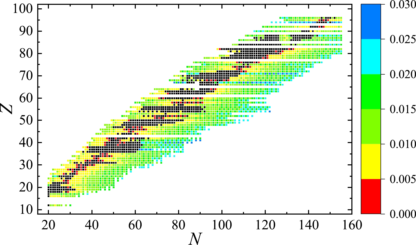
Figure 3. (color online) Theoretical uncertainties
$\sigma^{\rm pre}$ (in fm) of our predicted nuclear charge radii ($\sigma^{\rm pre} < 0.03$ fm), based on the CR2013 database [18]. The black squares denote nuclei with experimental data. -
To summarize, in this paper, we improve the
$ \delta R_k $ relations proposed in Ref. [55] by considering a term that relates to Z and the parity of N to reduce the deviations correlating to the odd-even difference of N and combine the improved$ \delta R_k $ with the$\delta R_{i { n} - j { p}}$ relations. These two types of relations are proved to be efficient in describing and predicting charge radii for nuclei with$ N \geq 20 $ and three abnormal regions excluded and are applied to predict 2467 unknown nuclear charge radii with theoretical uncertainties below 0.03 fm, based on the CR2013 database [18]. These predictions are tabulated in the Supplemental Material [62]. In addition, the structure evolutions of nuclei around$ N = 60 $ , 89, and 107 reflected from our improved relations are also discussed.
Predictions of nuclear charge radii
- Received Date: 2023-03-01
- Available Online: 2023-08-15
Abstract: In this study, we improve the relations of the charge-radius difference of two isotopes by considering a term that relates to the proton number and the parity of the neutron number. The correction reduces the root-mean-squared deviation to 0.0041 fm for 651 nuclei with a neutron number larger than 20, in comparison with experimental data compiled in the CR2013 database. The improved relations are combined with local relations consisting of the charge radii of four neighboring nuclei. These combinations also prove to be efficient in describing and predicting nuclear charge radii and can reflect the structure evolutions of nuclei. Our predictions of 2467 unknown nuclear charge radii at competitive accuracy, which are calculated using these two types of relations, are tabulated in the Supplemental Material.


 DownLoad: