


 Abstract
 HTML
HTML Reference
 Related
 PDF
PDF


-
Synthesis of 9Be involves overcoming the well-known gap with A = 8. Therefore, the 9Be as the seed nucleus may be incorporated in branching chains leading to carbon isotope production. More than 30 years have passed since Malaney and Fowler raised the issue of 9Be production and suggested additions to the standard nuclear reaction network for developing the inhomogeneous model of Big Bang nucleosynthesis (BBN) [1]. While discussing the role of the radioactive isotopes in the formation of stable elements at the early stage of the evolution of the Universe, a set of chains has been proposed (see the network in Fig. 1 of Ref. [2]). Later, two chains essential for the production of neutron-rich isotopes were suggested in [3]:
$ \begin{aligned}[b]\\[-8pt]{}^{4}{\rm{He}}(^{3}{\rm H},\gamma)^{7}{\rm{Li}}(n,\gamma)^{8}{\rm{Li}}(\alpha,n)^{11}{\rm B}(n,\gamma)^{12}{\rm B}({\rm e}^-{\rm ν})^{12}{\rm C}(n,\gamma)^{13}{\rm C}(n,\gamma)^{14}{\rm C}(n,\gamma)^{15}{\rm C}({\rm e}^-{\rm ν})^{15}{\rm N}…, \end{aligned}\tag{1a}$ 
$ ^{7}{\rm{Li}}(n,\gamma)^{8}{\rm{Li}}(n,\gamma)^{9}{\rm{Li}}({\rm e}^-{\rm ν})^{9}{\rm{Be}}(n,\gamma)^{10}{\rm{Be}}({\rm e}^-{\rm ν})^{10}{\rm B}(n,\gamma)^{11}{\rm B}(n,\gamma)^{12}{\rm B}({\rm e}^-{\rm ν})^{12}{\rm C}…. \tag{1b}$

Path (1a) is the Lithium-Boron-Carbon (Li-B-C) chain, and (1b) is the Lithium-Berillium-Boron-Carbon (Li-Be-B-C) chain. Reaction 9Be(n,γ)10Be in (1b) plays the role of trigger for ignition of the B-C path. That is reasonable as 10Be is a long-lived isotope (1.387×10⁶ years) and, therefore, may play the role of seed nucleus. One may find the balance between the (1a) and (1b) scenarios while all corresponding reaction rates are well-defined.
There is one more matter of concern for the 9Be(n,γ)10Be process: Terasawa and coworkers raised the issue of the critical reaction flows leading to the production of carbon isotopes (Fig. 6 in Ref. [4]). It was pointed out in [4] that the switch-off of the 10Be(α,γ)14C reaction in the Be-isotope chain leads to the ignition of the Li-Be-C reaction flow:
$ ^{7}{\rm{Li}}(n,\gamma)^{8}{\rm{Li}}(n,\gamma)^{9}{\rm{Li}}({\rm e}^-{\rm ν})^{9}{\rm{Be}}(n,\gamma)^{10}{\rm{Be}}(n,\gamma)^{11}{\rm{Be}} (n,\gamma)^{12}{\rm{Be}}({\rm e}^-{\rm ν})^{12}{\rm B}({\rm e}^-{\rm ν})^{12}{\rm C}…. \tag{1c} $ 
We will pay special attention to the 9Be(n,γ)10Be reaction in the beryllium paths (1b) and (1c). Our motivation concerns the disputed point of view on the origin of 10Be: The current position is that 10Be cannot be produced by thermonuclear reactions in stars [5] but is processed via cosmic-ray spallation [6]. Meanwhile, the rate of the 9Be(n,γ)10Be reaction is included in the network for calculation of the abundance of the beryllium isotopes in the context of BB nucleosynthesis up to CNO [7, 8].
The role of the 9Be(n,γ)10Be reaction in chains (1b) and (1c) is still unclear today. The reason is that only one modeless result on the reaction rate published by Rauscher in 1994 [9] was included in the network calculations [7]. Nowadays, there are two more reports on the reaction rate based on model calculations [10, 11]. Below we show that these results do not confirm those of Ref. [9]. The present paper, along with [10, 11], is intendedto attract attention to the 9Be(n,γ)10Be reaction and reconsider its astrophysical status in the evolution of the elements according to (1b) and (1c) branching.
We propose the practical goal of reproducing the cross-sections of nucleon-induced radiative capture reactions on the 1p-shell nuclei (A≤16) within the same model approach, an ad hoc modified potential cluster model (MPCM), and finally to calculate the corresponding reaction rates [12, 13] in order to complete the sequences like (1). Recently we presented calculations on the reactions 7Li(n,γ)8Li [14], 10B(n,γ)11B [15], 11B(n,γ0)12B [16], and 11B(n,γ0+1+2+3+4)12B [17].
The preliminary research on the 9Be(n,γ)10Be reaction that we conducted nearly ten years ago [18] should be recognized as estimative for the following reasons:
(a) The cross-sections for the capture to the ground state (GS) and four excited states (ESs) have been calculated in the energy range of 10 meV (1 meV = 10−3 eV) up to 1 MeV. Only two experimental points at 25 meV [19] and 25 keV [20, 21] were available as benchmarks.
(b) Only one
${}^3{D_3}$ resonance at 622 keV in l.s. was considered in [18]. Extension of the energy interval from 1 MeV to 5 MeV allows the inclusion of four more resonances in the present treatment. Their effect on the cross-sections and the reaction rates is demonstrated.(c) The calculation procedure of the overlapping integrals is re-examined compared to [18] (see for details Sec. VI).
(d) The reaction rate is not calculated in [18].
In the present work within the MPCM, we consider the 9Be(n,γ0+1+2+3+4+5)10Be reaction in the region of thermal and astrophysical energies of 10 meV up to 5 MeV, considering the formation of 10Be in both the GS and five ESs below n9Be threshold and the five lowest resonances. Present research on 9Be(n,γ)10Be also covers new experimental data on the thermal neutron capture cross-section [22−24]. Theoretical calculations are now relevant, while the experimental study of the 9Be(n,γ)10Be reaction is insufficient. Recent measurements of the total cross-section
$\sigma (E)$ for this reaction added two points [10]; therefore, six points are available now above 1 MeV [10, 20, 21].We also compare the MPCM reaction rate with model calculations [9] and direct radiative capture model results [10, 11].
The present work is organized as follows: Section I presents the Introduction. Section II covers calculation methods. A classification of orbital states and interaction potentials are given in Sec. III and Sec. IV, respectively. Section V presents the total cross-sections, and Sec. VI provides the reaction rates. The conclusions follow in Sec. VII.
-
We provided a detailed presentation of MPCM in [17, 25] (see references therein). Generally, the nuclear wave function (WF) is constructed as the antisymmetrized product of the internal cluster functions, consisting of A1 and A2 nucleons and a relative motion function [26]. These WFs are characterized by specific quantum numbers, including JLS and Young's diagrams {f}, and they determine the orbital part of WF permutation symmetry of the relative motion of the clusters.
The MPCM is easy to use since it comes down to solving the two-body problem, equivalent to the one-body problem in a central field. For the scattering states, the potentials are constructed based on the description of the scattering phase shifts or the spectra of the final nucleus, with consideration of the main low-lying resonances. For a bound state (BS) of two clusters in a nucleus, the interaction potentials are primarily constructed based on the requirement to describe the main characteristics of the nucleus. In this case, the potential parameters from the known characteristics of the BS of nuclei are fixed.
The obtained continuum and discrete WFs are the constituents for the calculation of the integral cross-section
$\sigma (NJ,{J_f})$ of the A(a,γ)B reactions. The calculation formalism for EJ and MJ transitions in the potential cluster model is described in [12, 13]. The partial total cross-sections of radiative capture from the initial Ji state in the continuous spectrum to the final bound Jf state are of the form$ \sigma (NJ,{J_f}) = \frac{{8\pi K{{\rm e}^2}}}{{{\hbar ^2}{k^3}}}\frac{{\text{μ }}}{{(2{S_1} + 1)(2{S_2} + 1)}}\frac{{J + 1}}{{J{{[(2J + 1)!!]}^2}}}A_J^2(NJ,K) \times \sum\limits_{{L_i}\,,{J_{i\,}}} {P_J^2(NJ,{J_f},{J_i})I_J^2(k,{J_f},{J_i}).} $

(2) Here,
$\mu $ is the reduced mass of particles in the initial channel, and k is the wave number of particles in the initial channel.${S_1}$ and${S_2}$ are the spins of particles in the initial channel. K and J are the wave number and total momentum of the$\gamma $ quantum, respectively. NJ denotes the electric EJ or magnetic MJ transitions of the J multipolarity from the initial${J_i}$ state in the continuous spectrum to the final bound${J_f}$ state of the nucleus.For electric orbital ЕJ(L) transitions, the values of
${P_J}$ ,${A_J}$ , and${I_J}$ are defined as [12, 13]:$\begin{aligned}[b] P_J^2(EJ,{J_f},{J_i}) =& {\delta _{{S_i}{S_f}}}\left[ {(2J + 1)(2{L_i} + 1)(2{J_i} + 1)(2{J_f} + 1)} \right]\\&\times{({L_i}0J0|{L_f}0)^2}\left\{ {\begin{array}{*{20}{c}} {{L_i}} \\ {{J_f}} \end{array}\begin{array}{*{20}{c}} S \\ J \end{array}\begin{array}{*{20}{c}} {{J_i}} \\ {{L_f}} \end{array}} \right\}{,^2}\end{aligned} $

(3) $ {A_J}(EJ,K) = {K^J}{\mu ^J}\left( {\frac{{{Z_1}}}{{{m^J}_1}} + {{( - 1)}^J}\frac{{{Z_2}}}{{{m^J}_2}}} \right), $

(4) $ {I_J}(k,{J_f},{J_i}) = \left\langle {{\chi _f}\left| {{r^J}} \right|{\chi _i}} \right\rangle . $

(5) Here,
${L_f},{L_i},{J_f},{J_i}$ are the orbital and total angular momentums of the particles in the initial (i) and final (f) channels;${m_1},~{m_2},~{Z_1},~{Z_2}$ are the masses and charges of the particles in the initial channel; and${I_J}(k,{J_f},{J_i})$ is the integral over the initial${\chi _i}$ and final${\chi _f}$ relative motion radial functions and part of the ЕJ(L) operator.To consider the magnetic МJ(S) transitions, we use the following expressions:
$ \begin{aligned}[b] P_J^2(MJ,{J_f},{J_i}) =& {\delta _{{S_i}{S_f}}} [ S(S + 1)(2S + 1)(2{J_i} + 1)\\&\times(2{L_i} + 1)(2J - 1) {(2J + 1)(2{J_f} + 1)} ] \\& \times {({L_i}0J - 10|{L_f}0)^2}{\left\{ {\begin{array}{*{20}{c}} {{L_i}}&{J - 1}&{{L_f}} \\ S&1&S \\ {{J_i}}&J&{{J_f}} \end{array}} \right\}^2}, \\ \end{aligned} $

(6) $\begin{aligned}[b] {A_J}(MJ,K) =& \frac{{\hbar K}}{{{m_0}c}}{K^{J - 1}}\sqrt {J(2J + 1)}\\&\times \left[ {\mu _1^{}{{\left( {\frac{{m_2^\,}}{{m_1^\, + {m_2}}}} \right)}^J} + {{( - 1)}^J}\mu _2^{}{{\left( {\frac{{m_1^\,}}{{m_1^\, + {m_2}}}} \right)}^J}} \right], \end{aligned}$

(7) $ {I_J}(k,{J_f},{J_i}) = \left\langle {{\chi _f}} \right|{r^{J - 1}}\left| {{\chi _i}} \right\rangle . $

(8) We use the following input data: particle masses in the atomic mass unit (amu)
${m_n}$ = 1.00866491597 [27],$m({}^9{\rm{Be}})$ = 9.0121829 [28], and the constant$ {\hbar ^2}/{m_0} = $ 41.4686 MeV·fm2, where${m_0}$ − amu. Magnetic moments are${\mu _1} \equiv {\mu _n} = - 1.91304272{\mu _0}$ and${\mu _2} \equiv \mu ({}^9{\rm{Be}}) = - 1.778{\mu _0}$ .Selection rules for the corresponding angular momentums are provided by the Clebsch-Gordan coefficients, 6j − and 9j − symbols in (3) and (6) according to [29]. All numerical calculations in the present study have been performed based on our authorial software using Simply Fortran. Most of these programs are included in the books in their updated form [12, 13].
-
Consider the classification of orbital states of clusters based on Young's diagrams for the 9Be nucleus. Assuming that this system consists of 8 + 1 particles, we can use diagrams {44} and {1} for them. In this case, for 9Be, we obtain two possible orbital symmetries, {54} + {441}. The first is forbidden since it contains five cells in one row, and the second is allowed. The diagram {441} corresponds to the allowed states (AS) in the n8Be system.
Therefore, for the n9Be system, we have {441} + {1} = {541} + {442} + {4411}. This set contains forbidden states (FS) with the diagram {541} for the orbital angular momentums L = 1, 2, 3,… and AS with configuration {4411} and L = 1, 3. Orbital angular momentums L are determined by Elliott's rule [30, 31]. Diagram {442} is apparently an allowed one with L = 0, 2,… and is relevant to allowed BSs in S and D waves. We limited our treatment to the minimum values of the orbital angular momentum L = 0, 1, 2.
The quantum numbers of 9Be are
${J^{\text{π }}} = 3/{2^ - }$ , and for 10Be, they are${J^\pi },T = {0^ + },1$ [32, 33]. The n9Be potential refers to the${}^3{P_0}$ wave corresponding to Young's diagrams {541} and {4411}. The first diagram is forbidden, and the second is allowed. The diagram {4411} matches the GS of the 10Be nucleus in the n9Be channel. The other${}^3{P_J}$ waves correspond to the allowed bound excited states. Similar potentials are used for the continuous partial waves.We assume that there is a bound AS for the {442} diagram in the
${}^3S$ wave without FS. It may correspond to the third excited state (3rd ES) with${J^\pi } = {1^ - }$ and excitation energy of 5.9599 MeV.In the
${}^3D$ wave containing a bound FS for the {541} diagram, there is also a bound AS for {442}. It may correspond to the fifth excited state (5th ES). The same classification is done for all other partial waves. Therefore, we unambiguously fix the structure of the forbidden and allowed states in each partial potential for L = 0, 1, 2. Note that the number of BSs, forbidden or allowed in any partial potential, determines the number of WF nodes at short distances [26]. Recall that the radial bound state function corresponding to the minimum energy has no node, and the BS next highest in energy has one node, etc. [34]. -
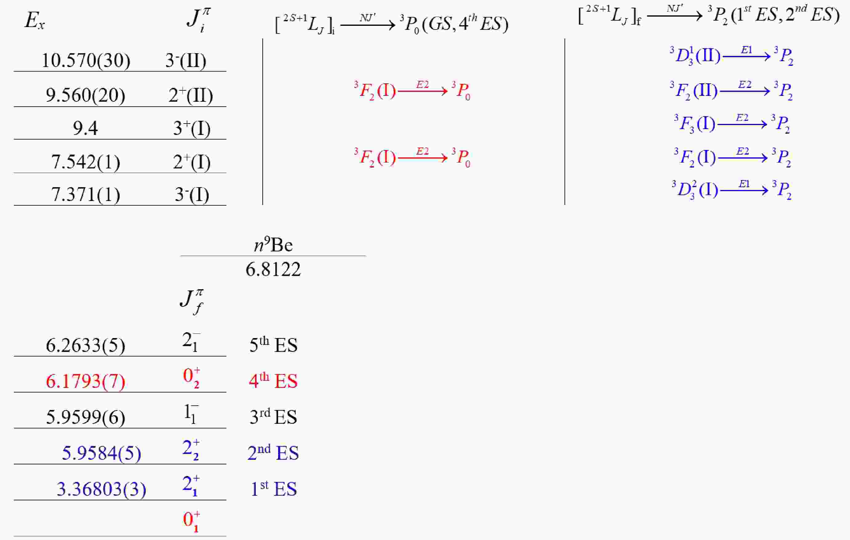
Figure 1 illustrates the spectrum of the 10Be nucleus and guides our further calculations. It shows six BSs, ad hoc one GS, and five ESs. Five resonances above the threshold Eb = 6.8122 MeV are included in the consideration.
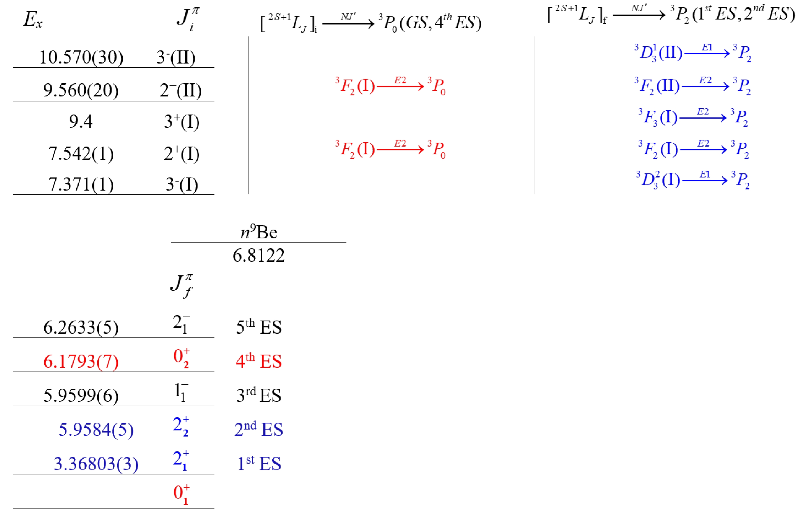
Figure 1. (color online) Spectrum levels in MeV (c.m.) of the 10Вe nucleus with the indication of quantum numbers
${J^\pi },T$ [32, 33] (arbitrary energy scale).$J_{\mathbf{N}}^\pi $ – low index N = 1 or 2 indicates the order of appearance of the state with the same momentum$J$ in the spectrum of 9Be. In the case of a continuous spectrum, the corresponding indication is given as a Roman numeral.To calculate the cross-sections (2), one needs to construct the discrete and scattering radial functions in overlapping integrals
$ {I_J}({J_f},{J_i}) $ (5) and (8). Functions$ {\chi _i} $ and$ {\chi _f} $ are the numerical solutions of the radial Schrödinger equation with the inter-cluster potentials of the Gaussian form:$ V(r,JLS) = - {V_0}(JLS)\exp \{ - \gamma (JLS){r^2}\}, $

(9) Here,
${V_0}$ is potential depth, and γ is related to the potential width. The procedure of fitting${V_0}$ and γ for the discrete and continuous states is presented in the following sub-sections. -
The BS parameters
${V_0}$ and γ are found unambiguously by matching the binding energy, charge radius, and AC. While the binding energy and charge radius can be calculated with high accuracy, the most significant uncertainties are due to AC. Let us start with the definition of AC. The dimensionless constant$ {C_w} $ is found from the following relation:$ {{{\chi }}_L}(r) = \sqrt {2{k_0}} {C_w}{W_{ - \eta L + 1/2}}(2{k_0}r). $

(10) Here,
$ {W_{ - \eta L + 1/2}} $ is the Whittaker function and$ {k_0} $ is a wave number related to the binding energy${E_b} = {k_0}^2/2\mu $ . In case$\eta = 0$ , the analytical form of the Whittaker function is:$ {W_{0,l}}(z) = {{\rm e}^{ - z/2}}\sum\limits_{n = 0}^l {{z^{ - n}}} \frac{{(l + n)!}}{{(l - n)!n!}}. $

(11) Let us present all variants for the ACs, which include the asymptotic normalization coefficient (ANC), dimensionless asymptotic constant
${C_w}$ , and spectroscopic factor$ {S_F} $ . The dimensional asymptotic constant C (in fm-1/2) is related to ANC via the spectroscopic factor$ {S_F} $ :$ A_{\rm NC}^2 = {S_F} \times {C^2} . $

(12) Along with relation (10), the asymptotics of WF may be written via the dimensional constant C
$ {{{\chi }}_L}(r) = C{W_ - }_{\eta L + {\text{1}}/{\text{2}}}\left( {{\text{2}}{k_0}r} \right) . $

(13) Comparison of relations (10) and (13) shows the following interrelation of the asymptotic constants:
$ C = \sqrt {2{k_0}} {C_w}. $

(14) The available information on the spectroscopic factors
$ {S_F} $ and ACs$A_{\rm NC}^2$ for the GS of 10Be is given in Table 1 [11, 35−46]. The relation$C_w^2 = A_{\rm NC}^2/({S_F}2{k_0})$ is used for the calculation of values${C_w}$ . In Table 2, we present the data on the spectroscopic factors${S_F}$ for the virtual decay of 10Be* in ESs: the experimental values are from [35–39, 45, 46] and the calculated ones from [11, 40−44].Reference $ {S_F} $ 

$ {C_w} $ 

Experiment Bockelman et al., 1951 [36], Variational method 2.357 2.231 Darden et al., 1976 [37], DWBA 2.1 2.07 Harakeh et al., 1980 [38], DWBA 1.58 1.81 Lukyanov et al., 2014 [39], Optical model 1.65 1.85 Average, present calculations ${ {\bar{\boldsymbol S} }_{\boldsymbol{F} } } \bf{=1.922}$ 

${ {\bar{\boldsymbol C}}_{\boldsymbol{w} } } {\bf = 1.990}$ 

Theory Schmidt-Rohr et al., 1964 [40], Born Approximation 1.67 1.89 Cohen & Kurath, 1967 [41], 1p shell model 2.3565 2.231 Anderson et al., 1974 [42], DWBA 1.21 1.54 Mughabghab, 1985 [43], Spin-spin interaction 2.1 2.07 Ogawa et al., 2000 [44], Stochastic variational method 2.24 2.14 Lee et al., 2007 [45], Shell model 2.44 2.30 Grinyer et al., 2011 [46], Shell model 2.62 2.41 Grinyer et al., 2011 [46], ab initio 2.36 2.23 Grinyer et al., 2011 [46], Variational Monte Carlo 1.93 2.01 Timofeyuk, 2013 [35], 0-p shell model 1.515 1.77 Mohr, 2019 [11], Direct capture model ~1.06 1.36 Mohr, 2019 [11], Direct capture model 1.58 1.81 Average, present calculations ${ {\bar{\boldsymbol S}}_{\boldsymbol{F} } } {\bf =1.923}$ 

${ {\bar{\boldsymbol C}}_{\boldsymbol{w} } } {\bf =1.980}$ 

Table 1. Data on the spectroscopic factors
${S_F}$ and calculated constants$ {C_w} $ for the GS of 10Be ($J_{\mathbf{N}}^\pi $ =$0_1^ + $ ) corresponding to$A_{\rm NC}^2$ = 9.12 fm−1 [35].Reference 1st ES, $2_1^ + $ 

2nd ES, $2_2^ + $ 

3rd ES, $1_1^ - $ 

4th ES, $0_1^ + $ 

5th ES, $2_1^ - $ 

Experiment Bockelman et al., 1951 [36], Variational method 0.274 0.421 ‒ ‒ ‒ Darden et al., 1976 [37], DWBA 0.23 ≤1.0 ‒ ‒ 0.065 Harakeh et al., 1980 [38], DWBA 0.38 ≤0.73 ≤0.14 ‒ 0.08 Lukyanov et al., 2014 [39], Optical model 1.00 1.40 0.43 ‒ 0.26 Average 0.471 0.888 0.285 ‒ 0.135 Theory Schmidt-Rohr et al., 1964 [40], Born Approximation 0.24 ‒ ‒ ‒ ‒ Cohen & Kurath, 1967 [41], Shell model 0.1261 0.1899 ‒ ‒ ‒ Anderson et al., 1974 [42], DWBA 0.17 0.54 0.36 ‒ 0.20 Mughabghab, 1985 [43], Spin interaction 0.23 ‒ ‒ 0.031 ‒ Ogawa et al., 2000 [44], Variational method 0.23 0.40 0.79 0.10 ‒ Mohr, 2019 [11], Direct capture model 0.38 <0.73 <0.14 ‒ 0.08 Mohr 2019 [11], Direct capture model 0.17 0.54 ‒ ‒ ‒ Average 0.2209 0.4800 0.43 0.0655 0.14 Table 2. Data on the spectroscopic factors
${S_F}$ for the ESs of 10Be*.The calculated results on the binding energy Eb, charge Rch, and matter radii Rm within the MPCM are presented in Table 3.
No. ${E_x}$ /MeV

${J^\pi }$ 

${\left[ {{}^{2S + 1}{L_J}} \right]_f}$ 

${V_0}$ /MeV

${E_b}$ /MeV

Rch/fm Rm/fm ${C_w}$ 

1 0 $0_1^ + $ 

${}^3P_0^1$ 

363.351572 −6.81220 2.53 2.54 1.72(1) 2 3.36803(3) $2_1^ + $ 

${}^3P_2^1$ 

345.676475 −3.44417 2.54 2.57 1.14(1) 3 5.9584(5) $2_2^ + $ 

${}^3P_2^2$ 

328.584340 −0.85380 2.55 2.69 0.60(1) 4 5.9599(6) $1_1^ - $ 

${}^3{S_1}$ 

33.768513 −0.85230 2.56 2.76 1.24(1) 5 6.1793(7) $0_2^ + $ 

${}^3P_0^2$ 

326.799005 −0.63290 2.56 2.72 0.53(1) 6 6.2633(50) $2_1^ - $ 

${}^3{D_2}$ 

248.148914 −0.54890 2.53 2.52 0.057(1) For the potential of the GS binding energy, the value 6.812200 MeV is obtained with an accuracy of 10–6 MeV, the mean square charge radius equals 2.53 fm, and the matter radius is 2.54 fm. The AC error is determined by averaging over the interval 4 – 16 fm, where the AC remains practically stable.
The potential of the first excited state (1st ES)
$^3P_2^1$ at an excitation energy of 3.36803(3) MeV 10Be [–3.44417] is obtained with${J^\pi } = {2^ + }$ . Here and further in brackets, the energy relative to the threshold n9Be is pointed in MeV. Such potential has one bound FS at {541}. Since data on the AC of this and other ESs are absent, the parameter γ is the same as for the GS potential.For the potential of the second excited state (2nd ES)
$^3P_2^2$ at an excitation energy of 5.9584(5) MeV, 10Be [–0.85381] with${J^\pi } = {2^ + }$ is obtained. It also has one FS.At an excitation energy of 5.9599(6) MeV [–0.8523], the third excited state (3rd ES) with quantum numbers
${J^\pi } = {1^ - }$ is reported in Ref. [32]. Such an excited state we consider as a bound AS in the${}^3{S_1}$ wave related to the {422} Young's diagram.The fourth excited state (4th ES) at an energy of 6.1793(7) MeV [–0.6329] coincides in its quantum numbers
${J^\pi },$ $T = {0^ + },1$ with the GS [32].The fifth excited state (5th ES) at an energy of 6.2633(50) MeV relative to the GS [–0.54890] with quantum numbers
$2_1^ - $ refers to the${}^3{D_2}$ state [32]. We did not consider the 5th ES earlier [18], and here, we estimate the value of its contribution to the total n9Be capture cross-sections.While calculating the charge and matter radii of 10Be, a 9Be nucleus radius equal to the 2.518(12) fm from Ref. [47] was used. The neutron charge radius equals zero, and its matter radius is the same as the proton radius 0.8775(51) fm given in the database [27]. To demonstrate the quality of present calculations of the Rch charge and Rm matter radii, we suggest compiling the experimental data on these values and available model calculations in Table 4.
Reference States Rm/fm Rch /fm Experiment Ozawa et al. 2001 [48], Glauber Model 2.30±0.02 2.30±0.02 Nörtershäuser et al. 2009 [49], Isotopic shift GS, $0_1^ + $ 

2.357(18) 2.357(18) Descouvemont & Itagaki 2020 [50], Stochastic variational method 2.44±0.02 2.44±0.02 Average values 2.3657±0.02 2.3657±0.02 Theory Liatard et al. 1990 [51], Microscopic model 2.479±0.028 ‒ Ogawa et al. 2000 [44], Stochastic variational method 2.28 2.35 Wang et al. 2001 [52], Relativistic Mean Field GS, $0_1^ + $ 

2.40 ‒ Timofeyuk, 2013 [35], 0-p shell model ‒ 3.042 Ahmad et al. 2017 [53], Glauber Model 2.36±0.04 ‒ Average values 2.3798±0.034 2.696 Ogawa et al. 2000 [44], Stochastic variational method 1st ES, $2_1^ + $ 

2.41 3.47 Table 4. Data on the Rch charge and Rm matter radii.
The summary of the spectroscopic factor SF and Cw for the GS of 10Be shows very close average values for the experimental (
${\bar S}^{\text{exp.}}_F = 1.922$ ,${\bar C}^{\text{exp.}}_w = 1.99$ ) and theoretical (${\bar S}^{\rm theor.}_F = 1.923$ ,${\bar C}^{\rm theor.}_w = 1.98$ ) ones. At the same time, the corresponding intervals differ. In the case of experiment one has:$1.58 \leqslant {\bar S}^{\text{exp.}}_F \leqslant 2.357$ and$1.85 \leqslant {\bar C}^{\text{exp.}}_w \leqslant 2.23$ , and the theoretical intervals are$1.06 \leqslant {\bar S}^{\rm theor.}_F \leqslant 2.62$ and$1.36 \leqslant {\bar C}^{\rm theor.}_w \leqslant 2.41$ . The value for the asymptotic constant Cw for the GS of 9Be obtained in present calculations equals 1.72(1), which is within the indicated intervals.There are no data on the ANC for the excited states of 10Be. The obtained Cw in Table 3 may be assumed as the proposed ones for the 1st – 5th ESs.
Based on the interaction potentials with parameters from Table 3, the radial wave functions of the BSs have been calculated as the numerical solutions of the radial Schrödinger equation. The description of the developed algorithm may be found in Refs. [25, 54].
The BS radial WFs are shown in Fig. 2. Their node or nodeless behavior is the signature of the Young's diagram classification relative to the number of ASs and FSs in a given partial wave. These functions are the constituents of the overlapping integrals (5) and (8).
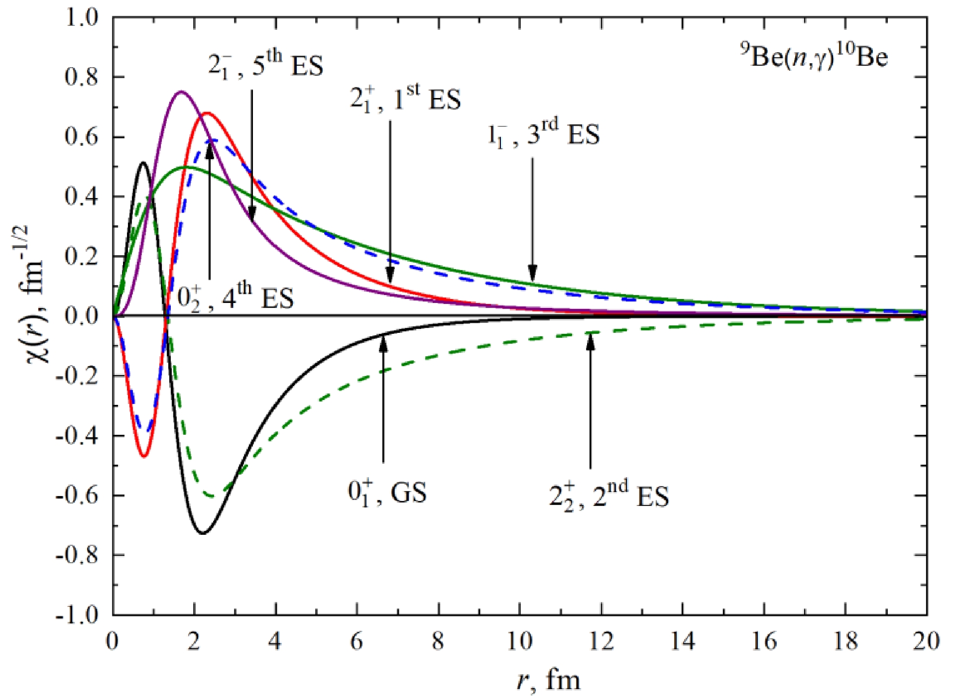
Figure 2. (color online) Radial wave functions of the bound states in the n9Be channel calculated with the potentials from Table 3.
-
Following Fig. 1, we consider five resonance states of n9Be at energies less than 5.0 MeV. We use the characteristics of the energy levels to construct the scattering potentials: By fitting the excitation energy
${E_x}$ and level width${\Gamma _{\rm c.m.}}$ , the parameters${V_0}$ and γ are determined. The results for the matched parameters of the scattering potentials are given in Table 5. The calculated values of the${E_{\rm res}}$ and${\Gamma _{\rm c.m.}}$ are in good agreement with the experimental data [32, 33].No. ${E_x}$ , expt.

${\Gamma _{\rm c.m.} }$ , expt.

Jπ ${}^{2S + 1}{L_J}$ 

${V_0}$ /MeV

γ/ fm-2 ${E_{\rm res} }$ , theory

${\Gamma _{\rm c.m.} }$ , theory

1 7.371(1) 15.7(5) 3- $^3D_3^1$ 

457.879 0.35 0.559(1) 15(1) 2 7.542(1) 6.3(8) 2+(I) $^3F_2^1$ 

211.667 0.11 0.730(1) 6(1) 3 9.4 291(20) 3+ $^3{F_3}$ 

220.685 0.12 2.588(1) 283(1) 4 9.560(20) 141(10) 2+(II) $^3F_2^2$ 

337.83 0.18 2.748(1) 146(1) 5 10.570(30) 200(100) 3- $^3D_3^2$ 

1953.33 1.5 3.758(1) 187(1) 6 No res. – 1– $^3{D_1}$ 

300.0 0.35 – – 7 No res. – 1+ $^3{P_1}$ 

206.0 0.4 – – Table 5. Parameters of the potentials of the resonant and nonresonant scattering states in the n9Be channel. The excitation energy of
${E_x}$ (MeV) levels and their width${\Gamma _{\rm c.m.}}$ (keV) are taken from experimental data [32, 33]. Resonance energies${E_{\rm res}}$ (MeV) and widths${\Gamma _{\rm c.m.}}$ (keV) are calculated with the parameters${V_0}$ and γ.Let us comment on Table 5 and its illustration in Fig. 3. In the spectrum of the 10Be nucleus in the n9Be channel, there is an above-threshold
${J^\pi } = {3^ - }$ level at the energy of 0.622(1) MeV in l.s. or 0.559(1) keV in c.m. and width of${\Gamma _{\rm c.m.}} = 15.7$ keV [32]. We compare it to the resonance$^3D_3^{\,1}$ in the elastic n9Be scattering channel.
For the potential of the resonance
$^3D_3^{\,1}$ scattering wave at 559(1), the corresponding keV parameters are the same as in [18]. The elastic scattering phase shift for this potential is shown in Fig. 3 by a solid red curve and has a resonance character, reaching 90(1)° at 559(1) keV. The potential contains the bound FS related to the diagram {541} following the above classification, and the state for {422} is considered unbound. The width of such a resonance is equal to 15(1) keV, which is in good agreement with the results of Ref. [32].The next
${J^\pi } = {2^ + }$ resonance at an excitation energy of 7.542(1) MeV relates to the resonance at 0.730 MeV c.m. and width of${\Gamma _{\rm c.m.}} = 6.3(8)$ keV. We failed to find potential parameters correctly conveying the characteristics of such a resonance in the P wave. We found the potential with FS for the${}^3{F_2}$ wave, which allows us to reproduce the${J^\pi } = {2^ + }$ resonance characteristics. The elastic scattering${}^3{F_2}$ phase shift is shown in Fig. 3 by a solid magenta curve and illuminates a resonance behavior, reaching 90(1)° at 730(1) keV.Consider a resonance at an excitation energy of 9.4 MeV
${J^\pi } = {3^ + }$ . It relates to the resonance at 2.588 MeV c.m. and a width of 291(20) keV. We consider this state a 3F3 wave. The corresponding potential contains one FS that leads to the resonance at 2.588(1) MeV c.m. and a width of 283(1) keV. The scattering phase shift$\delta_F $ (2.588 MeV) = 90(1)° (solid green curve in Fig. 3).The next resonance is located at an excitation energy of 9.560 (20) MeV
${J^\pi } = {2^ + }$ . It relates to the$^3F_2^{}$ wave with a resonance at 2.748(20) MeV c.m. and a width of 141(10) keV. The corresponding potential contains one FS and gives Eres = 2.748(1) MeV and Γc.m.= 146(1). The scattering phase shift$\delta_F$ (2.748 MeV) = 90(1)° (solid blue curve in Fig. 3).We associate the last
${J^\pi } = {3^ - }$ resonance at an excitation energy of 10.570(30) MeV with the${}^3D_3^2$ wave with a resonance at 3.758(30) MeV c.m. and width of 200(100) keV. It leads to resonance at 3.758 (1) MeV c.m. and a width Γc.m. = 187 (1) keV. The scattering phase shift$\delta_D $ (3.758 MeV) = 90(1)° (the solid cyan curve in Fig. 3).The potential of the
${}^3{D_1}$ scattering wave leads to zero scattering phase shifts since no resonances are observed in this state. This potential contains a bound FS corresponding to the {541} diagram, and the state for {422} is not bound.The parameters of the potentials for the nonresonant
${}^3{P_{0,2}}$ waves are the same as for the BSs from Table 3, and for the${}^3{P_1}$ wave, the values are indicated in Table 5.For the
${}^3{S_1}$ scattering wave, the parameters of interaction potential from Table 3 are used.We do not consider here the resonances at 9.27 MeV with
${J^\pi } = {4^ - }$ [32], 10.150 MeV, and 11.800(50) MeV with${J^\pi } = {4^ + }$ [33]. They only lead to the E2 transitions, which give a noticeably smaller contribution to the cross-sections, unlike E1 transitions.For the resonant waves, the relation between the scattering phase shift
$\delta $ and the resonance width value${\Gamma _{\rm c.m.}}$ is as follows:$ {\Gamma _{\rm c.m.}} = 2{({\rm d}\delta /{\rm d}{E_{\rm c.m.}})^{ - 1}}. $

(15) Figure 3 illustrates the corresponding phase shifts calculated with the potentials from Tables 3 and 5.
-
The partial cross-sections are calculated from (2) – (8) and presented in Fig. 4(a). The selection rules for the allowed transitions are provided by the vector addition of angular momentums in Clebsch-Gordan coefficients, the 6j and 9j-symbols in expressions (3) and (6). The summary of the multiple NJ transitions is presented in Table 6. The factor
$P_J^2(NJ,{J_f},{J_i})$ in the final column shows the algebraic weight of the corresponding amplitude in a partial cross-section. Fig. 4(b) compares the present MPCM calculations with those from [11] discussed below.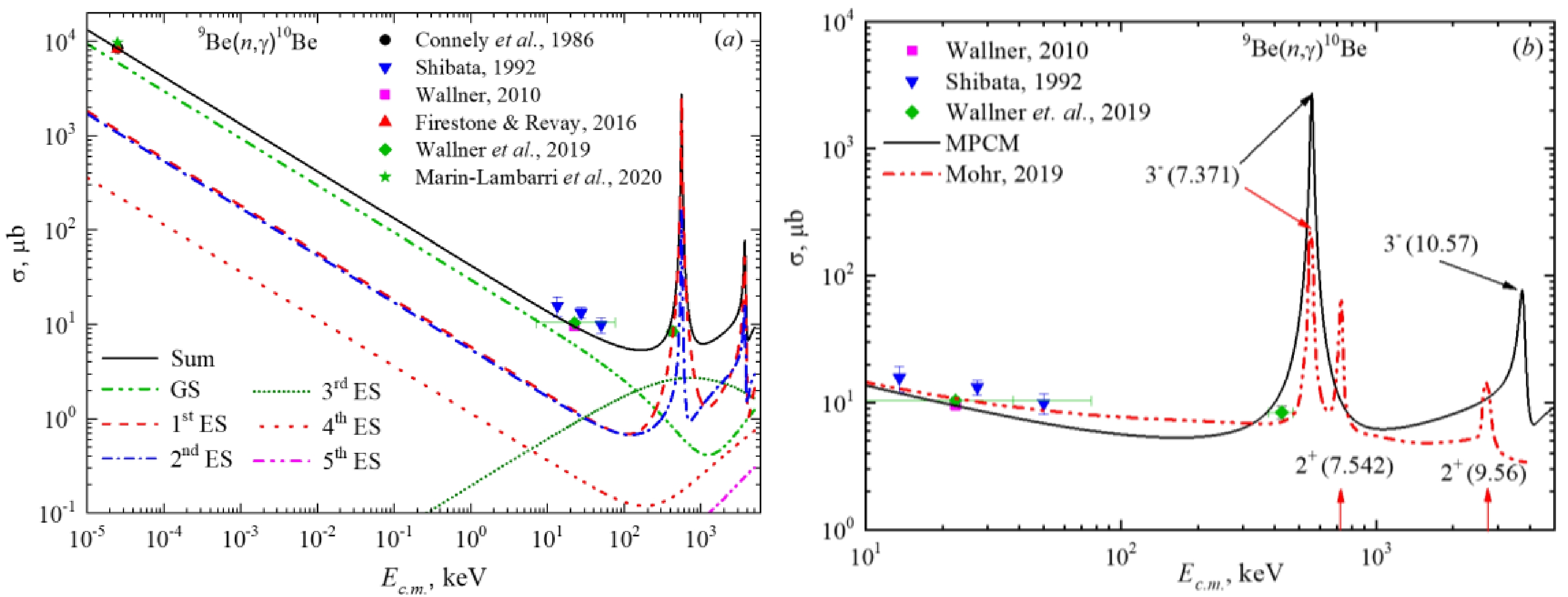
Figure 4. (color online) Total cross-sections for the reaction of radiative n9Be capture. Experimental data:
No. [2S+1LJ]i NJ transitions [2S+1LJ]f $P_J^2(NJ,J_f^{},{J_i})$ 

GS (green dot-dotted curve in Fig. 4(a)) 1 $^3{S_1}$ (No. 4 Table 3)

E1 $ { }^{t} \mathbb{P}_{\mathrm{t}}^{\mathrm{d}} $ 

1 2 $^3{D_1}$ (No. 6 Table 5)

E1 $ { }^{t} \mathbb{P}_{\mathrm{t}}^{\mathrm{d}} $ 

2 3 3P1 (No. 7 Table 5) M1 $ { }^{t} \mathbb{P}_{\mathrm{t}}^{\mathrm{d}} $ 

2 4 $^{\mathbf{3}}{{\mathbf{F}}_{\mathbf{2}}}$ (No. 2, No. 4 Table 5)

E2 $ { }^{t} \mathbb{P}_{\mathrm{t}}^{\mathrm{d}} $ 

3 1st ES (red dashed curve in Fig. 4(a)) 5 3S1 (No. 4 Table 3) E1 $ { }^{2} P_{2} $ 

5 6 3D1 (No. 6 Table 5) E1 $ { }^{2} P_{2} $ 

1/10 7 3D2 (No. 6 Table 3) E1 $ { }^{2} P_{2} $ 

3/2 8 ${}^{\mathbf{3}}{\mathbf{D}}_{\mathbf{3}}^{\mathbf{1}}$ (No. 1 Table 5)

E1 $ { }^{2} P_{2} $ 

42/5 9 ${}^{\mathbf{3}}{\mathbf{D}}_{\mathbf{3}}^{\mathbf{2}}$ (No. 5 Table 5)

E1 $ { }^{2} F_{2} $ 

42/5 10 3P1 (No. 7 Table 5) M1 $ { }^{2} F_{2} $ 

5/2 11 3P2 (No. 2 Table 3) M1 $ { }^{2} F_{2} $ 

15/2 12 $^{\mathbf{3}}{{\mathbf{F}}_{\mathbf{2}}}$ (No. 2, No. 4 Table 5)

E2 $ { }^{2} F_{2} $ 

3/7 13 $^{\mathbf{3}}{{\mathbf{F}}_{\mathbf{3}}}$ (No. 3 Table 5)

E2 $ { }^{2} F_{2} $ 

3 2nd ES (blue dash-dotted curve from Fig. 4(a)) 14 $^3{S_1}$ (No. 4 Table 3)

E1 $ { }^{2} \mathbb{R}_{2}^{2} $ 

5 15 $^3{D_1}$ (No. 6 Table 5)

E1 $ { }^{2} \mathbb{R}_{2}^{2} $ 

1/10 16 $^3{D_2}$ (No. 6 Table 3)

E1 $ { }^{2} \mathbb{R}_{2}^{2} $ 

3/2 17 ${}^{\mathbf{3}}{\mathbf{D}}_{\mathbf{3}}^{\mathbf{1}}$ (No. 1 Table 5)

E1 $ { }^{2} \mathbb{R}_{2}^{2} $ 

42/5 18 ${}^{\mathbf{3}}{\mathbf{D}}_{\mathbf{3}}^{\mathbf{2}}$ (No. 5 Table 5)

E1 $ { }^{2} \mathbb{R}_{2}^{2} $ 

42/5 19 3P1 (No. 7 Table 5) M1 $ { }^{2} \mathbb{R}_{2}^{2} $ 

5/2 20 3P2 (No. 3 Table 3) M1 $ { }^{2} \mathbb{R}_{2}^{2} $ 

15/2 21 $^{\mathbf{3}}{{\mathbf{F}}_{\mathbf{2}}}$ (No. 2, No. 4 Table 5)

E2 $ { }^{2} \mathbb{R}_{2}^{2} $ 

3/7 22 $^{\mathbf{3}}{{\mathbf{F}}_{\mathbf{3}}}$ (No. 3 Table 5)

E2 $ { }^{2} \mathbb{R}_{2}^{2} $ 

3 3rd ES (dark cyan short dotted curve in Fig. 4(a)) 23 3P0 (No. 1 Table 3) E1 $ { }^{2} F_{1} $ 

1 24 3P1 (No. 7 Table 5) E1 $ { }^{2} F_{1} $ 

3 25 3P2 (No. 2 Table 3) E1 $ { }^{2} F_{1} $ 

5 4th ES (red dotted curve in Fig 4(a)) 26 $^3{S_1}$ (No. 4 Table 3)

E1 $ { }^{2} P_{6}^{2} $ 

1 27 3D1 (No. 6 Table 5) E1 $ { }^{2} P_{6}^{2} $ 

2 28 3P1 (No. 7 Table 5) M1 $ { }^{2} P_{6}^{2} $ 

2 29 $^{\mathbf{3}}{{\mathbf{F}}_{\mathbf{2}}}$ (No. 2, No. 4 Table 5)

E2 $ { }^{2} P_{6}^{2} $ 

3 5th ES (magenta dash-dot-dotted curve in Fig. 4(a)) 30 3P1 (No. 7 Table 5) E1 3D2 9/2 31 3P2 (No. 2 Table 3) E1 3D2 3/2 Table 6. Classification of partial transitions for the 9Be(n,γ0+1+2+3+4+5)10Be reaction. In column 2, the indicated initial scattering state [2S+1LJ]i is supplied with the number of the corresponding potential with parameters given in the indicated table. Resonance transitions are indicated with bold. The final state is noted as [2S+1LJ]f.
$P_J^2$ are the algebraic factors (3) and (6).Within the constructed partial cross-section, we mark the transitions leading to the resonances in bold. These resonances occur via the strong E1 transition to the 1st and 2nd ESs, and they are observed in partial
$(n,{\gamma _1})$ and$(n,{\gamma _2})$ cross-sections in Fig. 4(a). The strength of the E2 transitions is much less than that of E1. The value of the E2 cross-sections does not exceed 0.1 μb, so the resonance structure does not appear within the treated energy range.The partial capture
$(n,{\gamma _0})$ to the GS of 10Be provides the major background for all other partial cross-sections due to the E1 transition from the non-resonance${}^3{S_1}$ scattering wave not damped by the centrifugal barrier. Similar transitions can be seen for the capture to the 1st and 2nd ESs (No. 5 and 14 in Table 6). The partial cross-sections$(n,{\gamma _0})$ and$(n,{\gamma _4})$ are of the same structure.In our previous work [18], the radial matrix elements
${I_J}(k,{J_f},{J_i})$ defined in (5) and (8) were integrated only up to 20 fm, which is insufficient when the radial functions refer to the bound states with${E_{b}} < \,\,1\,{\text{MeV}}$ . These are 2nd – 5th ESs. Therefore, only GS and 1st ES integrals${I_J}(k,{J_f},{J_i})$ are calculated correctly, and all the others (2nd – 5th ESs) led to marked underestimates of the total cross-sections. Here, we have eliminated this inaccuracy and calculated the overlapping integrals (5) and (8) up to 100 fm.Note the results for the
$(n,{\gamma _0})$ and$(n,{\gamma _1})$ cross-sections do not practically differ from those obtained in [18]. Corrections inserted in the calculations of the$(n,{\gamma _2})$ ,$(n,{\gamma _3})$ , and$(n,{\gamma _4})$ cross-sections sometimes exceed the results of [18] by an order of magnitude.One more remark concerns the input of the
$(n,{\gamma _5})$ capture to the 5th ES into the total cross-section. It follows from Table 6 (No. 30 and 31 that despite the strong E1 transition, there are no resonances; therefore, the role of this partial cross-section is negligible.The experimental data for the total n9Be capture cross-sections are presented in [10, 19−23]. In Ref. [22], the experimental data for the cross-section at a thermal energy
${\sigma _{\rm th}}$ = 8.27(13) mb are reported. This value differs a little from the results of [19], where${\sigma _{\rm th}}$ = 8.49(34) mb, or [10] where${\sigma _{\rm th}}$ = 8.31(52) mb. The most recent measurements of the thermal cross-section give a value of${\sigma _{\rm th}}$ = 9.70(57) mb [23] and${\sigma _{\rm th}}$ = 9.70(53) mb [24]; they exceed the previous results by ~15%.Given certain general assumptions about the interaction potentials of the n9Be channel in the continuous and discrete spectrums, we describe the available experimental data on the total neutron capture cross-section at energies from 25 meV [19, 22] to the lower measured point at 426 keV [10, 20, 21] quite well. However, the early data from [55] at the Ec.m. energies ~12–45 keV (see comments in [10]) are higher than the latest results [10, 19−23].
Figure 4(a) illustrates the smooth increase of the total cross-section with the energy decrease. Low-energy approximation of the neutron radiative capture cross-sections without resonances may be found in [56]. At energies of 10-5 to 1 keV, the calculated cross-section shown in Fig. 4(a) by a solid curve may be approximated as follows:
$ \sigma (\mu{\rm b}) = \frac{A}{{\sqrt {{E_{\rm c.m.}}({\text{keV}})} }}. $

(16) Expression (16) refers to the S wave capture cross-section. The value of the constant A = 42.01 μb·keV1/2 is determined from one point in the total cross-sections at minimum energy, equal to 10−5 keV (c.m.). The corrected calculation of
${I_J}(k,{J_f},{J_i})$ integrals for the transitions to the 2nd and 4th ESs led to an increase in the coefficient A in expression (16) from 40.2 μb·keV1/2 [18] to 42.01 μb·keV1/2 by 4%.We consider the modulus of the relative deviation between the theoretical cross-section and its approximation by (16):
$ M(E) = \left| {[{\sigma _{\rm ap}}(E) - {\sigma _{\rm theor}}(E)]/{\sigma _{\rm theor}}(E)} \right| $

(17) in the energy range from 10−5 to 1 keV. Below 1 keV, the deviation M(E) does not exceed 0.9%. For example, the application of approximation (16) at 25.3 meV gives the value
${\sigma _{\rm th}}$ = 8.35 mb, which is within the error limits of the results of [19, 22].Let us comment on the only theoretical calculations of the total cross-sections of 9Be(n,γ0+1+2+3+4+5)10Be reaction performed in the folding cluster model [10,11] (see Refs. therein for the model formalism). In Fig. 4(b) we compare our total cross-section with calculations by Mohr [11], as they are in nearly the same energy interval. The results from Ref. [10] are very close to those of Mohr [11] and were obtained using the same approach.
In [11] four low-lying resonances corresponding to the states in 10Be at Ex = 7.371 MeV (
${J^\pi }$ , LJ = 3−, D3), 7.542 MeV (2+, P2), 9.27 MeV (4−, D4), and 9.56 MeV (2+, P2) are included. The 1st, 3rd, and 4th provide the resonance structure of the total cross section in Fig. 4(b) (red double-dotted curve). In our classification, 2+ resonances are associated with F-waves but not P-waves. This identification issue may be regarded as open. However, these 2+ states lead to the E2 capture cross-sections in both cases. As mentioned above, in our calculations, the E2 resonance capture cross-section does not exceed 0.1 μb; therefore, the results of Mohr [11] are unclear to us. We did not consider the 4− resonance due to its minor role. -
The corresponding reaction rates have been calculated based on the partial and summed cross-sections illustrated in Fig. 4(a). The present results are compared with the data on the reaction rate of Refs. [9−11].
The reaction rate for radiative neutron capture is calculated according to [57] in units of cm3mol−1s−1:
$\begin{aligned}[b] {N_A}\left\langle {\sigma v} \right\rangle =& 3.7313 \cdot {10^4}{\mu ^{ - 1/2}}T_9^{ - 3/2}\int\limits_0^\infty {\sigma (E)E}\\& \times\exp ( - 11.605E/{T_9}){\rm d}E . \end{aligned}$

(18) Here, the reduced mass μ is in amu, the temperature T9 in 109 K, the total cross section σ(E) in μb, and E in MeV. The integration was implemented over 100,000 points in the energy range 10-5 to 5·103 keV.
Figure 5 shows the calculated rate of the 9Be(n, γ0+1+2+3+4+5)10Be reaction with capture to the GS and all ESs. The partial contributions of transitions to different ESs are denoted in the figure field, and the black solid curve shows the total rate.
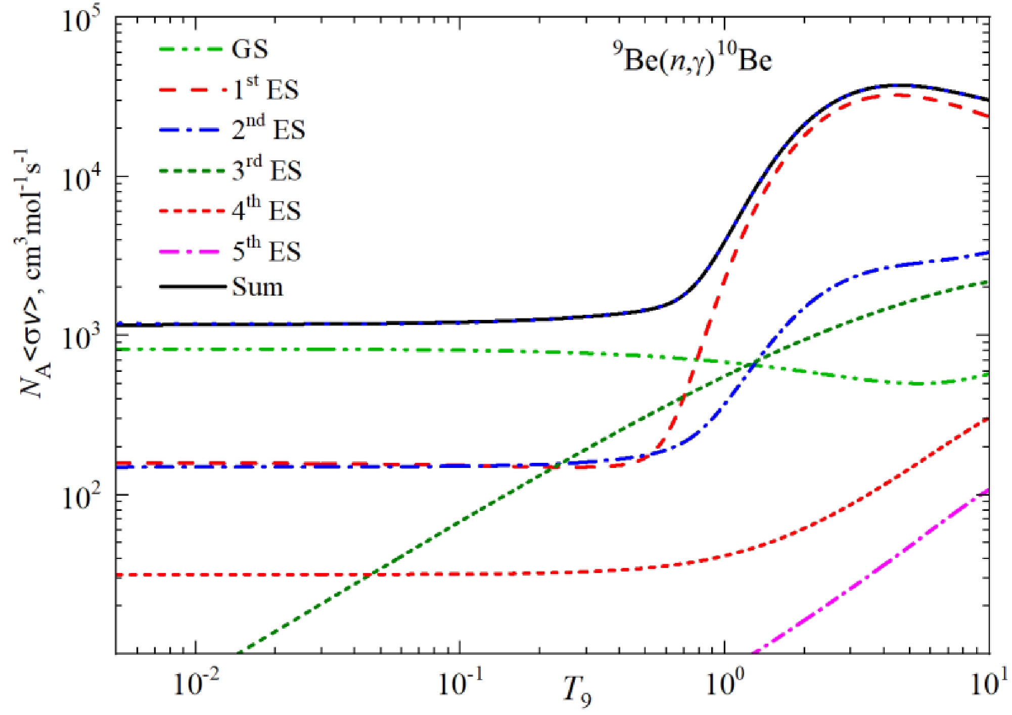
Figure 5. (color online) Total and partial reaction rates of neutron capture of the 9Be nucleus.
The total reaction rate is approximated by the analytical expression from [10]:
$\begin{aligned}[b] {N_A}\left\langle {\sigma v} \right\rangle =& {a_1}(1.0 + {a_2}T_9^{1/2} + {a_3}T_9^{} + {a_4}T_9^{3/2} + {a_5}T_9^2 + {a_6}T_9^{5/2})\\& + {a_7}/T_9^{3/2}\exp ( - {a_8}/T_9^{}). \end{aligned}$

(19) We provide the approximation parameters χ2 = 0.001 in Table 7. The accuracy of the calculated curve is 5%.
i ai i ai i ai i ai 1 1190.438 3 0.6435 5 0.00178 7 1.31549·106 2 –0.15943 4 –0.00344 6 –1.2853·10-4 8 6.4213 Table 7. Reaction rate approximation parameters.
We demonstrate in Fig. 6 the contributions of the resonance cross-sections to the total reaction rate. Comparison of
$ {\left\langle {\sigma v} \right\rangle _{{\text{res}}}} $ (black solid) and$ {\left\langle {\sigma v} \right\rangle _{{\text{non - res}}}} $ (red dashed) shows the rising of the total reaction rate from the ~ 0.4 T9. Their difference reaches an order of magnitude at the maximum at ~ 4 T9. Note that the non-resonance$ {\left\langle {\sigma v} \right\rangle _{{\text{non - res}}}} $ is calculated with the switched-off resonance amplitudes Nos. 4, 8, 9, 12, 13, 17, 18, 21, 22, and 29 of Table 5.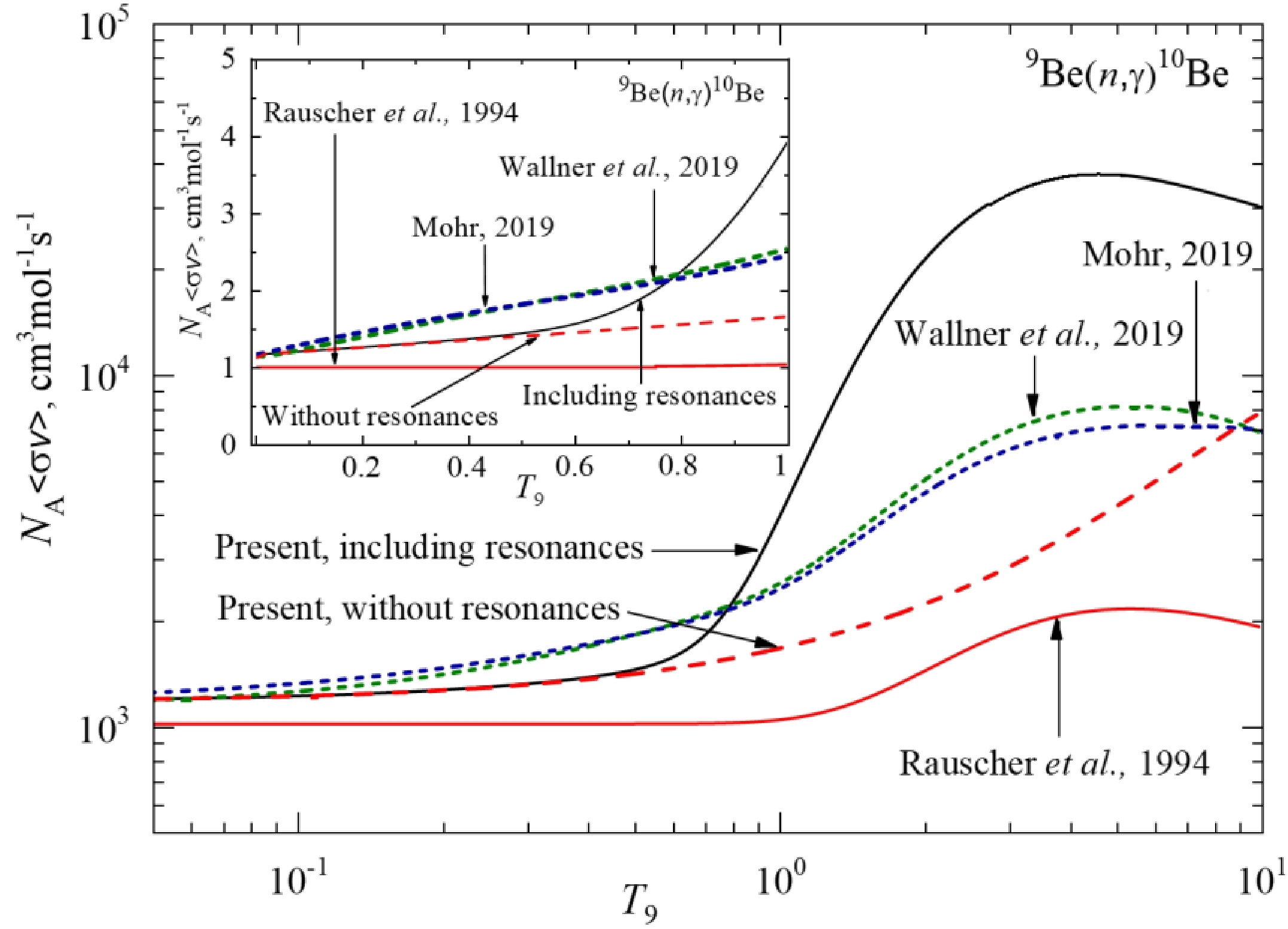
Figure 6. (color online) Comparison of the total reaction rates of radiative neutron capture of 9Be: the dark green short dashed curve is the result of Ref. [10], the blue short dashed curve is the result of Ref. [11], and the red solid curve is the result of Ref. [9]; the black solid curve is the total reaction rate including resonances (same as in Figure 5); and the red dashed curve is the result of present calculations without resonance amplitudes.
Another comment concerns the present calculations of the 9Be(n,γ0+1+2+3+4+5)10Be reaction rate and those from Refs. [10, 11] as well as [9]:
(i) Calculations of the total cross-sections in [10, 11] are performed in a folding cluster model but with subdivision into the direct capture part σDC and resonance part σR, ad hoc σ = σDC + σR ± 2(σDC·σR)1/2 cos(δR) [58, 59]. Contrariwise, in the MPCM approach, there is no such subdivision, and consequently there are no problems with uncertainties coming from the interference term. Both types of energy dependence are best viewed as continuous behavior of the scattering phase shifts 3D3, 3F2, and 3F3 in Fig. 3. Within this calculating scheme, the corresponding scattering functions χi are obtained and incorporated into the overlapping integrals (5) and (8). The calculations in [9] are modeless ones.
(ii) The most significant input into the cross-section at energies higher than ~ 500 keV comes from the first 3- (0.559) resonance. In [10, 11], to calculate the σR according to the Breit-Wigner formula, the experimental data on the first 3+ resonance state is exploited (see, for example, Table 2 in [11]). MPCM reproduces the parameters of this resonance also. In Refs. [10, 11], the value of σ(0.559 MeV) ≈ 200 μb is reported. In the present calculations, we obtained the value of σ(0.559 MeV) ≈ 1200 μb. This difference is illustrated in the corresponding reaction rates in nearly the same proportion: The present calculations exceed the reaction rates of [10, 11] starting from ~ 0.8 T9 and are higher by a factor of nearly 5 at ~ 5T9.
(iii) We confirm the conclusion of Mohr [11] on the temperature dependence of the reaction rate at the low-range T9 contrary to the constant
$ < \sigma v > $ behavior proposed in [9] (see insert in Fig. 6). -
The partial and total cross-sections of the 9Be(n, γ0+1+2+3+4+5)10Be reaction are calculated in the energy range from 10-5 to 5 MeV in the MPCM. The expansion of the energy range to 5 MeV allows us to consider five
$^3D_{\,3}^{\,1}$ ,$^3F_{\,2}^{\,1}$ ,$^3F_{\,3}^{}$ ,$^3F_{\,2}^{\,2}$ , and$^3D_{\,\,3}^{\,2}$ resonances and estimate their signature in the total cross-section. A narrow resonance of Ex = 0.730 MeV is proposed as an$^3F_2^1$ state, not a P one as in Ref. [11]. Comparing the GS partial cross-section, the transitions to the 1st and 2nd ESs contribute significantly to the total cross-section. The role of the (n,γ3) process increases with energy. The minor role of the (n,γ4) and (n,γ5) processes is demonstrated numerically.The calculated thermal cross-section
${\sigma _{\rm th}} = 8.35$ mb is in good agreement with experimental data of [10, 19−21], which are ~ 10% lower than the early measurements [23, 24]. That is cause for discussions with the experimentalists.The total and partial rates of the 9Be(n,γ0+1+2+3+4+5)10Be reaction are calculated in the temperature range of 0.001 to 10 T9 and are approximated by an analytical expression. The inclusion of resonances shows their impact on the corresponding reaction rate of a value higher by a factor of 4-5 at T9 >1 compared to the results of [10, 11].
The lack of experimental data on the cross-sections higher than 500 keV illustrates the problem of quantitatively reproducing the first 0.559 MeV resonance, as it makes the most significant contribution to the rate of the 9Be(n,γ)10Be reaction. New experimental measurements are strongly needed.
Finally, it is worth mentioning that our theoretical rstudy of the 9Be(n,γ)10Be reaction can be applied to the isobar-analog process 9Be(p,γ)10B. A comparative analysis of these processes within the same theoretical approach can illuminate the beryllium–boron branching under discussion.
Radiative 9Be(n,γ0+1+2+3+4+5)10Be reaction rate in the potential cluster model
- Received Date: 2023-04-21
- Available Online: 2023-08-15
Abstract: Within the framework of the modified potential cluster model with forbidden states, the total cross-sections of radiative n9Be capture to the ground and five low-lying excited states are calculated at energies from 10−2 eV up to 5 MeV. The thermal cross-section


 DownLoad: