


 Abstract
 HTML
HTML Reference
 Related
 PDF
PDF


-
According to recent observations [1, 2], the expansion of the universe appears to be accelerating, which is attributed to "dark energy," a mysterious substance that makes up approximately 70% of the total energy content of the universe, and the ΛCDM model is the most straightforward explanation for dark energy. However, it has issues such as "coincidence" [3], "fine-tuning" [4], and the "age" problem [5]. As a result, researchers have explored alternative possibilities for explaining the source and characteristics of dark energy, with scalar fields playing a significant role in several modified theories. In order to address these issues, it is reasonable to consider alternative possibilities that could explain the origin and nature of DE. Current descriptions of the evolution of the universe heavily rely on models involving scalar fields. In the past decade, a variety of DE models have been explored based on scalar field theories, including the quintessence, tachyon, phantom, K-essence, and Chaplygin gas models (for a comprehensive review, refer to [6] and the sources cited therein). Despite these efforts, a concrete and satisfactory DE model has yet to be developed.
Currently, the popular method for modeling late-time cosmic acceleration is called reconstruction, where observational data is directly incorporated into the model. This approach is essentially the opposite of the traditional method of finding a suitable cosmological model. Reconstruction of the universe can be accomplished using two different methods: parametric and non-parametric. Parametric reconstruction involves estimating model parameters from observational data, while non-parametric reconstruction is based on the statistical analysis of the observational data. Numerous studies have aimed to examine the evolution of the universe without depending on any particular cosmological model. Such approaches are referred to as model-independent methods of cosmological parametrization or cosmological models. This approach generally relies on the assumption of parametrizing geometrical parameters (such as the jerk parameter j, deceleration parameter q, Hubble parameter H, etc.) or physical parameters (in particular, the EoS parameter ω, pressure p, energy density ρ, etc.) to deduce precise solutions of Einstein field equations (see [7−17]).
If dark energy were not present, the universe would experience deceleration as a result of the gravitational force binding matter together, and this is upheld by the big bang nucleosynthesis and the theory of gravitational instability in structure formation. Thus, to provide an explanation for the formation of structures and the current measurements of acceleration, it is necessary to explain the transformation of the universe from deceleration to an acceleration phase. Thus, using a parametric approach to measure the evolution of the universe from a decelerating phase to an accelerating phase is reasonable. Furthermore, the use of a parametric approach can enhance the efficiency of future cosmological surveys. Previous studies have explored the kinematics of the universe using different parameterizations of the deceleration parameter (DP; see references [8−11,18−21]). Motivated by these facts, in this study we opted for a specific type of DP that results in a transition from the deceleration to the acceleration phase. The characteristics of this parameterization are explained in Sec. III, and to determine the model parameters, observational data from CC, BAO, and the recently released Pantheon
$ + $ datasets are utilized. The detailed statistical analysis of these data is given in Secs. IV and V. Further, using the results obtained from the statistical method, we interpret the behavior of the universe with our newly defined DP model (Sec. VI). -
The flat Friedmann-Lemaitre Robertson-Walker (FLRW) metric, which describes an isotropic and homogeneous universe, can be represented as
$ \begin{array}{*{20}{l}} {\rm d}s^2=-{\rm d}t^2+a^2(t)({\rm d}x^2+{\rm d}y^2+{\rm d}z^2). \end{array} $

(1) Here,
$ a(t) $ denotes the usual scale factor that determines the size of the expanding universe, which is related to the Hubble parameter as$ H=\dfrac{\dot{a}}{a} $ . The notation of the overhead dot represents differentiation with respect to the cosmic time variable t, and this convention is used consistently in this paper. Incorporating the FLRW metric into Einstein's field equations for a perfect fluid with total energy density ρ and isotropic pressure p yields the Friedmann equations for a spatially flat FLRW universe:$ 3H^2=\rho $

(2) $ 2\dot{H}+3H^2=-p, $

(3) where we have chosen units so that
$ 8\pi G=1 $ . The effective equation of state (EoS) parameter, denoted by ω, is given by the ratio of the pressure to the energy density, i.e.,$ \omega=\frac{p}{\rho}. $

(4) The behavior of the energy density and the expansion of the universe are directly related to ω. We note that if
$ \omega <-1/3 $ , the universe will experience acceleration. The use of the EoS parameter is not limited to distinguishing between the universe's decelerated and accelerated expansion phases; it can also be utilized to classify them. The epoch of matter domination is identified with a value of ω that equals zero. In the present epoch of accelerated expansion, ω values less than$ -1 $ correspond to the phantom age, and ω values that lie between$ -1 $ and$ -1/3 $ represent the quintessence phase.The evolution of the homogeneous and isotropic universe can be characterized by a fundamental parameter known as the deceleration parameter (DP), denoted by the symbol q, which is given by
$ q=-\frac{\ddot{a}}{H^2a}=-\left(\frac{\dot{H}}{H^2}+1\right). $

(5) The DP tells us the rate at which the expansion of the universe accelerates or decelerates. If q is greater than zero, it indicates retardation of expansion, while if q is less than zero, it indicates its acceleration. The Hubble parameter and the DP are connected through the relation
$ \begin{array}{*{20}{l}} H(z)=H_0 \exp \left(\int_0^z (q(\xi)+1){\rm d}\ln (\xi+1)\right), \end{array} $

(6) where
$ H_0 $ is the value of the Hubble parameter at$ z=0 $ , and z is the redshift, which is related to a by$ z=-1+\dfrac{1}{a} $ . -
Equations (2) and (3) present two systems of equations that involve three unknown parameters: ρ, p, and H. Therefore, to solve the system of equations, it is necessary to make an ansatz. In this direction, we assume a parametric form for the DP as a function of redshift z. Parametrization of the DP merits consideration for several reasons when compared to the parametrization of other kinematic models. One significant advantage is in terms of physical interpretation, particularly in relation to cosmic structure formation and the adherence of the universe to the second law of thermodynamics. A suitable parametric form for
$ q(z) $ can capture the behavior of cosmic expansion during different epochs and provide insights into the formation and evolution of large-scale structures. Additionally, to satisfy the requirements of cosmic structure formation, the deceleration parameter should approach$ 1/2 $ at high redshifts. This condition is crucial for ensuring that the universe undergoes the necessary deceleration during early stages, allowing structures to form and evolve over cosmic timescales. The second law states that the entropy of a closed system tends to increase or, at best, remain constant over time. In the context of cosmology, this law imposes constraints on the dynamics of the universe. For instance, one thermodynamic constraint is that the FLRW universe approaches thermodynamic equilibrium in the distant future, as discussed below. By considering the thermodynamic aspects of expansion, we can incorporate additional information into the parametrization of$ q(z) $ , ensuring that it satisfies thermodynamic constraints. Another compelling aspect of the parametrization of$ q(z) $ is its predictive power. By carefully choosing a suitable parametric form, we can accurately describe the past and present cosmic expansion and make reliable predictions about the future evolution of the universe. This predictive capability is particularly valuable for understanding the fate of the universe and its long-term behavior. By extrapolating the behavior of$ q(z) $ beyond the range of observed redshifts, we can gain insights into the future cosmic expansion, including whether it will continue to accelerate, eventually decelerate, or even undergo a transition to a different regime.Due to the significance of DP in the exploration of the universe, several authors have suggested parametrized forms of
$ q(z) $ based on both practical and theoretical considerations, as discussed in the introduction. However, some of these are only valid for certain redshift ranges (i.e., when$ z\ll 1 $ ) and others may not be predictive of future evolution. Motivated by these factors, we put forward a parametric expression for$ q(z) $ that remains finite for all$ z\in [-1,\infty] $ . Additionally, we require that$ q(z)\geq -1 $ for all$ z\in [-1,\infty] $ and$ q(z)\to -1 $ with$\dfrac{{\rm d}q}{{\rm d}z} > 0$ as$ z\to -1 $ , so that the FLRW universe approaches thermodynamic equilibrium in the distant future, as discussed in Campo et al. [10]. In addition, it is necessary for q to approach$ 1/2 $ at high redshifts to satisfy the requirements of cosmic structure formation. Taking these considerations into account, we present a broken polynomial form of DP given by:$ q(z)=-1+\frac{3}{2}\left( \frac{(a+z)^{(n-1)}(z+1)}{b+(a+z)^n}\right), $

(7) where a, b, and n are model parameters. The conditions
$ b>0 $ and$ n>1 $ must be imposed upon the preceding parametric form to ensure a divergence-free DP. Further, we must have$ a>1 $ so that$\dfrac{{\rm d}q}{{\rm d}z} > 0$ in the far future (i.e., as$ z\to -1 $ ). To ensure a more effective and reliable analysis, we limit our model to only two parameters by fixing a specific value for n. This approach is motivated by the challenges posed by higher-dimensional parameter spaces, including the increased likelihood of degeneracies where different parameter combinations yield similar observational outcomes. Such degeneracies hinder the unique determination of parameter values and can lead to inflated uncertainties and potentially misleading interpretations. Moreover, exploring high-dimensional spaces is computationally demanding and time-consuming, necessitating significant computational resources, whereas a smaller parameter space facilitates more efficient sampling and convergence checks. We observe that when$ n\neq 4 $ , the chosen parametrization described in Eq. (7) is influenced by prior effects. To mitigate this issue, we select$ n=4 $ for our analysis, resulting in a modified parametric form for the DP:$ q(z)=-1+\frac{3}{2}\left( \frac{(a+z)^{3}(z+1)}{b+(a+z)^4}\right). $

(8) This form incorporates a broken polynomial expression. The rationale behind adopting this broken polynomial form is rooted in the challenge of obtaining an analytic expression for the Hubble parameter
$ H(z) $ from Eq. (6).When
$ a>1 $ and$ b>0 $ , it is a simple matter to confirm that the DP meets the following criteria:$ \begin{align*} q(z)&\geq -1, \quad \text{ for all } z\in [-1,\infty],\\ q(z)&\to -1 \left(\text{and } \frac{{\rm d}q}{{\rm d}z}>0\right) \quad \text{ as } z\to -1,\\ q(z)&\to \frac{1}{2} \quad \text{ when } z \gg 1. \end{align*} $

By substituting the proposed ansatz for DP into Eq. (6), we deduce the expression for the Hubble parameter as follows:
$ H(z)=H_0\left(\frac{(a+z)^4+b}{a^4+b}\right)^{(3/8)}, $

(9) where
$ H_0 $ also appears as a free parameter in the preceding expression. Feeding the expression for the Hubble parameter into the Eqs. (2), (3), and (4) and recalling that$\dfrac{\rm d}{{\rm d}t}=-(z+1)H(z)\dfrac{\rm d}{{\rm d}z}$ , we obtain$ \rho(z)= \frac{3 c^2 \left((a+z)^4+b\right)^{3/4}}{\left(a^4+b\right)^{3/4}}, $

(10) $ p(z)=\frac{3 c^2 \left(-(a+z)^4+(z+1) (a+z)^3-b\right)}{\left(a^4+b\right)^{3/4} \sqrt[4]{(a+z)^4+b}}, $

(11) $ \omega(z)=-\frac{a^4+a^3 (3 z-1)+3 a^2 (z-1) z+a (z-3) z^2+b-z^3}{a^4+4 a^3 z+6 a^2 z^2+4 a z^3+b+z^4}. $

(12) As we can observe from Eq. (8), the DP q (as well as the derived quantities ρ, p, and ω) relies on the values of the parameters a and b. In order to explore the feasibility of a transition in the universe's expansion from deceleration to acceleration, we need to initially limit the potential values of the model parameters based on existing datasets. After obtaining the most suitable parameter values, we can then attempt to reconstruct DP q, and consequently ρ, p, and ω.
-
To construct a cosmological model that accurately reflects reality, it is necessary to limit the model parameters a, b, and the Hubble constant (
$ H_0 $ ) based on the available observational data. The present section provides an overview of the data sets used in the observational analysis and the statistical methods applied in this study. We rely on data from cosmic chronometers (CC), baryonic acoustic oscillations (BAO), and the latest Pantheon sample, called Pantheon$ + $ , derived from Supernovae type Ia (SNeIa) observations, to constrain our cosmological model. -
The CC method yields measurements of the Hubble rate by considering the oldest and most passively evolving galaxies, which are separated by a small redshift interval, based on the differential aging method. This uses the definition of the Hubble rate given by
$ H=-\frac{1}{1+z}\frac{{\rm d}z}{{\rm d}t}. $

(13) for an FLRW metric. The significance of the CC method is its ability to measure the Hubble parameter
$ H(z) $ independently of any cosmological assumptions, making it a valuable tool to test cosmological models.This study employs 31 data points compiled from Refs. [22−28], which were obtained using the CC method across a broad range of redshifts,
$ 0.1<z<2 $ . To perform the MCMC analysis, the chi-square function for the cosmic chronometers is given by$ \chi^2_{\rm CC}(\Theta)=\sum\limits_{i=1}^{31}\left[\frac{(H_{\rm th}(z_i,\Theta)-H_{\rm obs}(z_i))^2)}{\sigma_H^2(z_i)}\right], $

(14) where
$H_{\rm th}$ represents the Hubble parameter value for the model with model parameters Θ,$H_{\rm obs}$ represents the corresponding observed Hubble parameter, and$ \sigma_H $ represents the error in the observed value of H. -
The BAO peak is based on a comoving distance equal to the sound horizon at the drag epoch,
$ r_d $ . At a redshift z, the BAO peak position in the angular direction determines the angular separation$ \Delta \theta= r_d/((1+z)D_A(z)) $ , and in the radial direction, it determines the redshift separation$ \Delta z=r_d/D_H(z) $ , where$ D_A $ is the angular distance and$ D_H = c/H $ is the Hubble distance. Thus, by measuring the position of the BAO peak at any redshift, we can constrain the combinations of cosmological parameters that determine$ D_H/r_d $ and$ D_A/r_d $ , from which we can estimate$ H(z) $ by selecting an appropriate value of$ r_d $ . In this work, we use the 26 non-correlated data points coming from line-of-sight BAO measurements [29−40]. As with the CC method, the$ \chi^2 $ function for the BAO method reads$ \chi^2_{\rm BAO}(\Theta)=\sum\limits_{i=1}^{26}\left[\frac{(H_{\rm th}(z_i,\Theta)-H_{\rm obs}^{\rm BAO}(z_i))^2)}{\sigma_H^2(z_i)}\right], $

(15) where
$H_{\rm th}$ indicates the theoretical Hubble parameter values for the model with model parameters Θ,$H_{\rm obs}$ is the corresponding observed Hubble parameter from the BAO method, and$ \sigma_H $ is the error in the observed value of$H^{\rm BAO}$ .For the combined CC and BAO dataset, the
$ \chi^2_T $ function is defined as$ \begin{array}{*{20}{l}} \chi^2_T=\chi^2_{\rm CC}+\chi^2_{\rm BAO}. \end{array} $

(16) -
The Pantheon
$ + $ dataset [41−44] supplies distance moduli calculated from 1701 light curves of 1550 SNeIa within a redshift range of$ 0.001\leq z\leq 2.2613 $ , obtained from 18 different surveys. Notably, 77 of the 1701 light curves correspond to galaxies that contain Cepheids. One of the advantages of Pantheon$ + $ is that it can be used to constrain$ H_0 $ along with the model parameters. To fit the parameter of the model from the Pantheon$ + $ samples, we extremise the$ \chi^2 $ function$ \begin{array}{*{20}{l}} \chi^2_{\rm SNeIa}= \Delta\mu^T (C_{\rm stat+sys}^{-1})\Delta\mu, \end{array} $

(17) where
$C_{\rm stat+sys}$ is the covariance matrix of Pantheon$ + $ dataset formed by adding the systematic and statistical uncertainties and$ \Delta\mu $ is the distance residual given by$ \begin{array}{*{20}{l}} \Delta\mu_i=\mu_i-\mu_{th}(z_i), \end{array} $

(18) where
$ \mu_i $ is the distance modulus of the$i^{\rm th}$ SNeIa. Note that$ \mu_i=m_{Bi}-M $ , where$ m_{Bi} $ is the apparent magnitude of the$i^{\rm th}$ SNeIa and M is the fiducial magnitude of an SNeIa. The theoretical distance modulus$\mu_{\rm th}$ can be calculated from the following expression$ \mu^{th}(z,\Theta)=5\log_{10}\left(\frac{d_L(z,\Theta)}{1{\rm Mpc}} \right)+25, $

(19) where
$ d_L $ is the model-based luminosity distance in Mpc, which is given by$ d_L(z,\Theta)=\frac{c(1+z)}{H_0}\int_0^z \frac{{\rm d}\xi}{E(\xi)}, $

(20) where c is the speed of light and
$ E(z)=\dfrac{H(z)}{H_0} $ .When analyzing SNeIa data alone, there exists a degeneracy between the parameters H0 and M. To address this issue, a modification is made to the SNeIa distance residuals presented in Eq. (17), as shown in previous studies [42, 45]. Specifically, the modified residuals
$ {\Delta}{\tilde{\mu}} $ are defined as:$ \Delta\tilde{\mu}=\left\{\begin{array}{*{20}{l}} \mu_i-\mu_i^{\rm Ceph}, & \text{if}~~ i\in ~~ \text{ Cephied hosts}\\ \mu_i-\mu_{th}(z_i), & \text{otherwise} \end{array}\right. $

(21) where
$\mu_i^{\rm Ceph}$ indicates the Cepheid host of the$i^{\rm th}$ SNeIa as per SH0ES. It is to be noted that$\mu_i-\mu_i^{\rm Ceph}$ is sensitive to the Hubble constant$ H_0 $ and M. In our analysis, we take$ M=-19.253 $ as determined from SH0ES Cepheid host distances (see [41]).For joint observational constraints using the CC, BAO, and SNeIa datasets, the total
$\chi^2_{\rm tot}$ function is given as$ \begin{array}{*{20}{l}} \chi^2_{\rm tot}=\chi^2_{\rm CC}+\chi^2_{\rm BAO}+\chi^2_{\rm SNeIa}. \end{array} $

(22) Now, the best-fit parameters can be obtained by minimizing the
$ \chi^2 $ function. Since$ \chi^2 $ and likelihood are related by$ \mathcal{L} \propto \exp \left(-\frac{\chi^2}{2} \right) $ , minimizing the$ \chi^2 $ is equivalent to maximizing the likelihood, which is equivalent to minimizing the negative log-likelihood. Further, we utilize the Markov Chain Monte Carlo (MCMC) sampling technique and Python's emcee [46] library to obtain numerical constraints over the model parameters. The obtained results are presented in the form of contour plots up to$ 3 $ -σ ($ 99.7% $ ) confidence level. -
The observational data obtained through various cosmological surveys play a significant role in uncovering the dynamics of the universe. In the realm of parametric reconstruction, statistical analysis of the observed datasets provides a physically agreeable parameter space for free parameters. Employing the methodology for observational data discussed in the previous section, we now constrain model parameters a, b, and
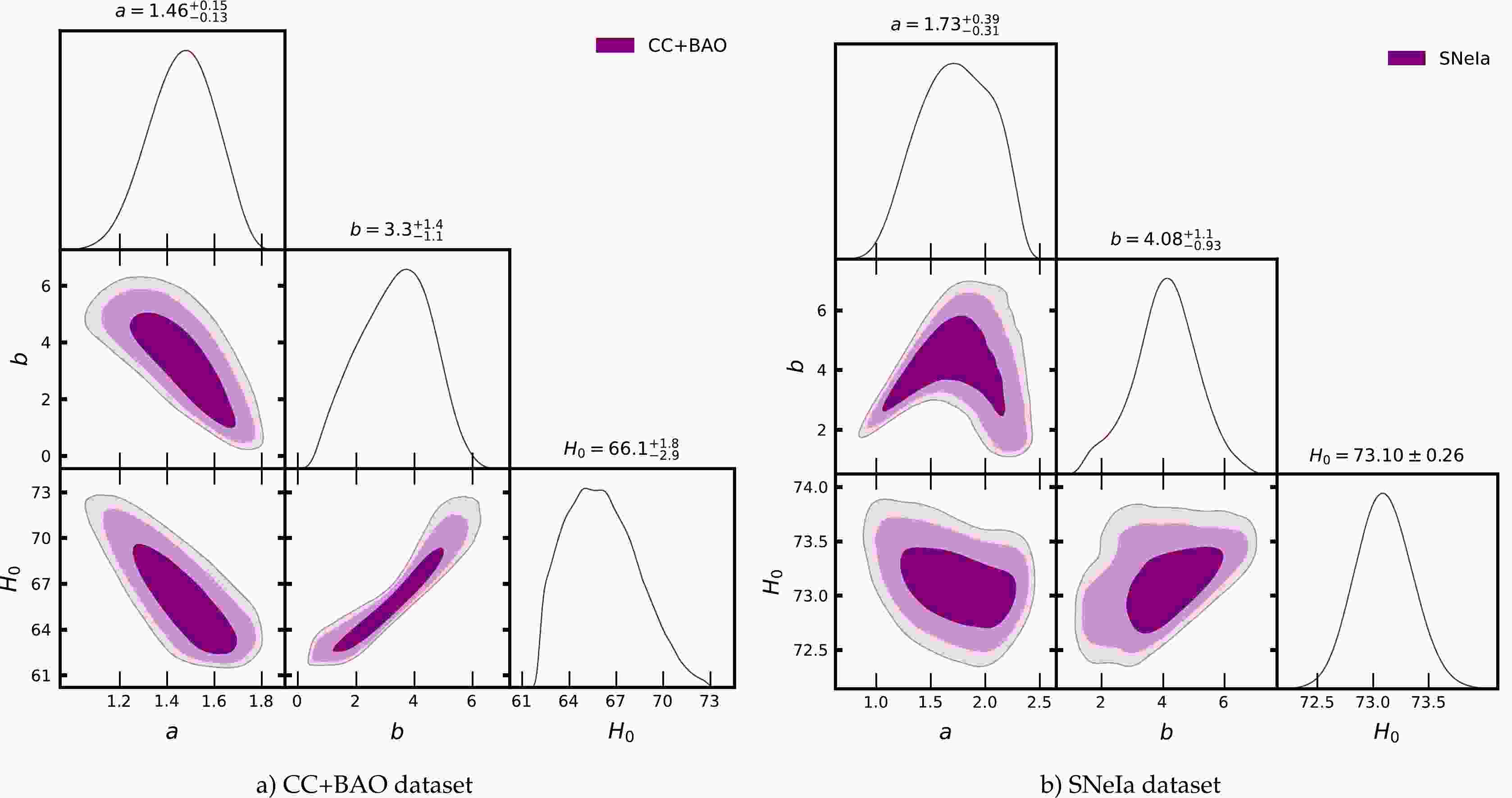
$ H_0 $ .The results of the MCMC analysis of the combined CC and BAO data for our model are displayed in Fig. 1(a), which shows
$ {1\sigma} $ -$ {3\sigma} $ likelihood contours along with the best fit and mean values of the model parameters. Thus, for combined CC and BAO, we find$ a=1.46^{+0.15}_{-0.13}, b=3.3^{+1.4}_{-1.1} $ , and$ {H_0}=66.1^{+1.8}_{-2.9} $ (with 1σ error). Fig. 1(b) depicts the 2D likelihood contours plot up to 3σ error for the 1701 data points of SNeIa. The best-fit values so obtained with 68% confidence levels are$ a=1.73^{+0.39}_{-0.31} $ ,$ b=4.08^{+1.1}_{-0.93} $ , and$ {H_0}=73.1\pm 0.26 $ . Similarly, the most agreeable values for model parameters with the combined CC, BAO, and SNeIa data points are$ a=1.319^{+0.073}_{-0.085} $ ,$ b=6.80^{+0.52}_{-0.62} $ , and$ H_0=74.22 \pm{0.21} $ (with 1σ error). Figure 2 provides the marginalized likelihood contours for CC+BAO+SNeIa data with 68%, 95%, and 99.7% confidence levels. The results of MCMC analysis with$ {1\sigma} $ -$ {3\sigma} $ errors for the different datasets are summarized in Table 1. In addition, for the ranges of values of the model parameters obtained from the respective datasets, we compare our parametric model with the ΛCDM model. Fig. 3(a) shows the behavior of our model (9) with respect to the redshift z. In Fig. 3(b), we plot the profile of the distance modulus (19). From these graphical representations, we can infer that our model agrees with the ΛCDM model. In the upcoming sections, we employ these values of the parameters to study the dynamics of the model.
Figure 1. (color online) Contour plot with
$ 1-\sigma $ ,$ 2-\sigma $ , and$ 3-\sigma $ errors for the parameters a, b, and$ H_0 $ along with the constraint values for the combined CC, BAO, and SNeIa datasets.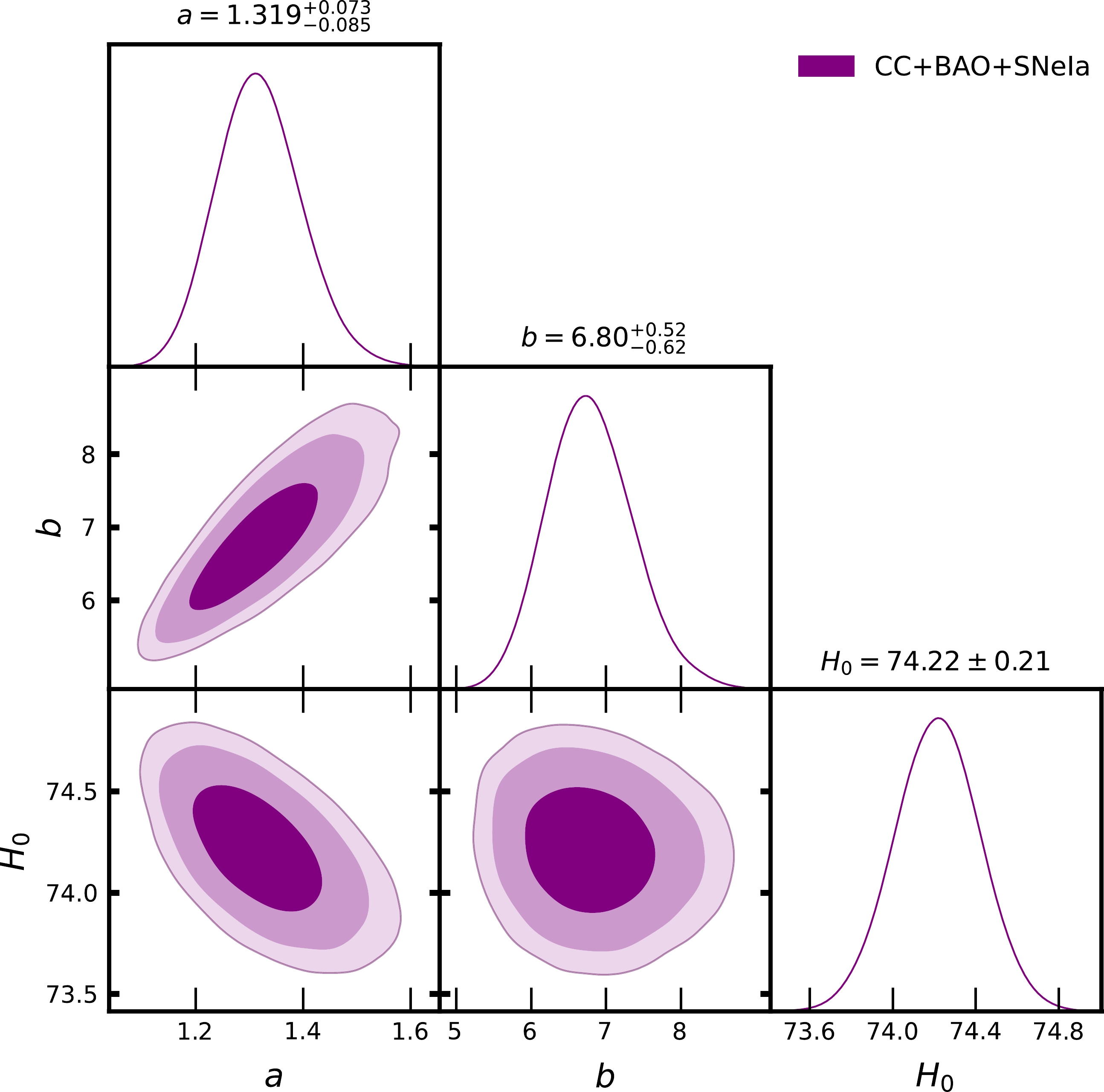
Figure 2. (color online) Contour plot with
$ 1-\sigma $ ,$ 2-\sigma $ , and$ 3-\sigma $ errors for the parameters a, b, and$ H_0 $ along with the constraint values for the combined CC, BAO, and SNeIa datasets.Dataset a b $ H_0 $ 

$ 1\sigma $ 

$ 1.46^{+0.15}_{-0.13} $ 

$ 3.3^{+1.4}_{-1.1} $ 

$ 66.1^{+1.8}_{-2.9} $ 

$ CC+BAO $ 

$ 2\sigma $ 

$ 1.46^{+0.26}_{-0.26} $ 

$ 3.3^{+2.2}_{-2.4} $ 

$ 66.1^{+4.2}_{-4.0} $ 

$ 3\sigma $ 

$ 1.46^{+0.30}_{-0.35} $ 

$ 3.3^{+2.7}_{-2.7} $ 

$ 66.1^{+5.7}_{-4.2} $ 

$ 1\sigma $ 

$ 1.73^{+0.39}_{-0.31} $ 

$ 4.08^{+1.1}_{-0.93} $ 

$ 73.1\pm0.26 $ 

SNeIa $ 2\sigma $ 

$ 1.73^{+0.58}_{-0.59} $ 

$ 4.10^{+2.0}_{-2.3} $ 

$ 73.1^{+0.51}_{-0.49} $ 

$ 3\sigma $ 

$ 1.73^{+0.64}_{-0.75} $ 

$ 4.10^{+2.6}_{-2.7} $ 

$ 73.1^{+0.68}_{-0.64} $ 

$ 1\sigma $ 

$ 1.319^{+0.073}_{-0.085} $ 

$ 6.80^{+0.52}_{-0.62} $ 

$ 74.22\pm0.21 $ 

CC+BAO+SNeIa $ 2\sigma $ 

$ 1.320^{+0.17}_{-0.15} $ 

$ 6.80^{+1.2}_{-1.1} $ 

$ 74.22^{+0.40}_{-0.41} $ 

$ 3\sigma $ 

$ 1.320^{+0.22}_{-0.19} $ 

$ 6.80^{+1.6}_{-1.3} $ 

$ 74.22^{+0.53}_{-0.53} $ 

Table 1. Results of MCMC for parameters a, b, and
$ H_0 $ (km/s/Mpc) with$ 1\sigma $ -$ 3\sigma $ errors.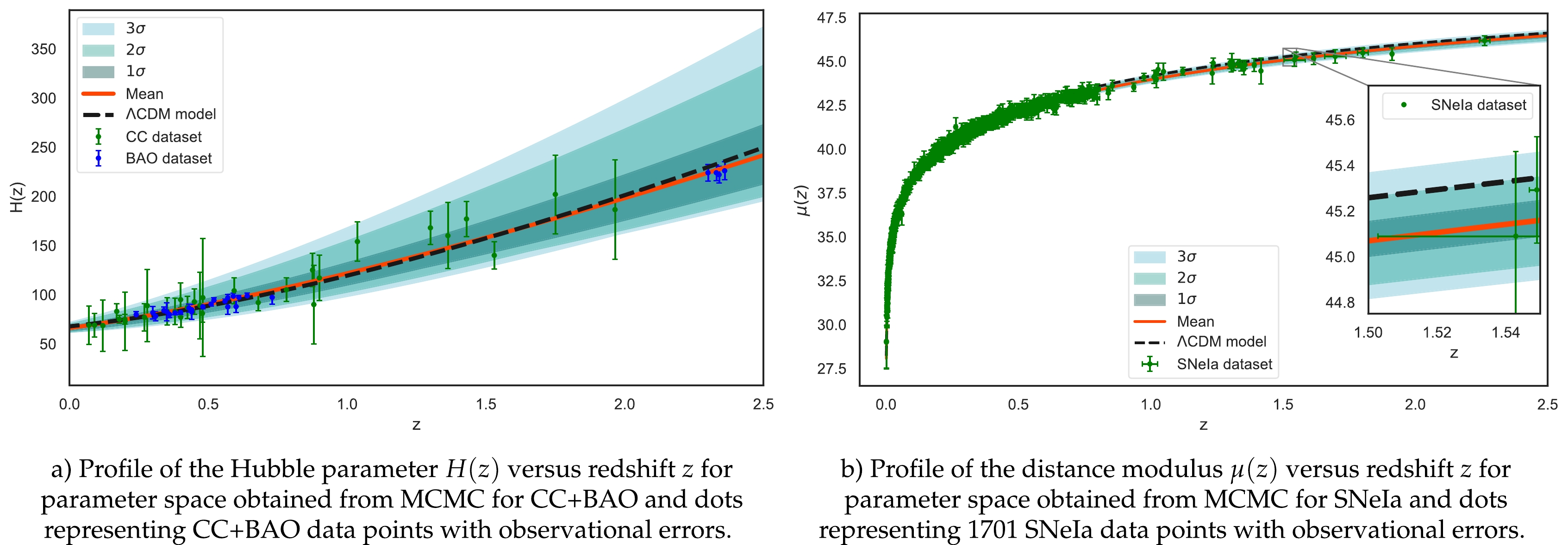
Figure 3. (color online) Comparison of the model for the obtained best-fits with the ΛCDM model (
$ \Omega_\lambda=0.7, \Omega_m=0.3, H_0= 67.8 $ ) with the observational data. -
The DP plays a crucial role in describing the dynamics of the universe and is considered one of the most important cosmological parameters. According to cosmological observations, the universe has undergone a cosmic speed-up in late times, indicating that it must have witnessed a slower expansion phase long ago. Additionally, a decelerating phase is equired for the formation of structures. The changeover of the universe from deceleration to acceleration, also known as the phase transition, is a crucial aspect that must be considered when describing the universe's dynamics. Estimating the current accelerating action of the universe involves evaluating negative values of the DP.
After taking all factors into account, we plot the graph of DP
$ q(z) $ with respect to z using the constrained values of the model parameters that we have obtained, and the results are presented in Fig. 4(a), 4(c), and 4(e). These figures clearly illustrate that our model generates late-time cosmic acceleration alongside a decelerated expansion in the past for all the constrained values of the model parameter. We also observed that the phase transition of the universe depends on the variation of the model parameters a and b. Moreover, the phase transition occurs at redshifts$ z_t = 0.636^{+0.214}_{-0.191} $ ,$ z_t=0.906^{+0.559}_{-0.304} $ , and$ z_t=0.894^{+0.048}_{-0.049} $ for the values of the constrained parameters deduced from the CC+BAO, SNeIa, and CC+BAO+ SNeIa datasets with 1-σ error, respectively. Notably, with regard to our current model, the transition redshift$ z_t $ values are in agreement with values attained by several other researchers using a variety of scenarios [11, 18, 47, 48]. Furthermore, it can be observed from Fig. 4(a), 4(c), and 4(e) that for the constrained parameters obtained from CC+BAO, SNeIa, and CC+BAO+SNeIa datasets, the present deceleration parameter values are$ q_0-0.405^{+0.762}_{-0.615} $ ,$ q_0=-0.404^{+0.046}_{-0.131} $ , and$ q_0=-0.649^{+0.062}_{-0.053} $ (with 1-σ error), respectively.
Figure 4. (color online) The nature of DP and effective EoS with the constraint values from various datasets.
The findings from Fig. 4(b), 4(d), and 4(f) suggest that in its current state, the universe is experiencing acceleration, as
$ \omega <-1/3 $ . The present value of ω is estimated to be approximately$ \omega_0 =-0.603^{+0.508}_{-0.410} $ ,$ \omega_0=-0.603^{+0.031}_{-0.087} $ , and$ \omega_0=-0.766^{+0.041}_{-0.035} $ , based on the 1-σ constrained parameter values obtained from the CC+BAO, SNeIA, and CC+BAO+SNeIa datasets, respectively. Further,$ \omega\geq -1 $ shows the quintessence phase of the universe. -
Energy conditions are crucial for understanding the singularity theorem, which plays a significant role in black-hole thermodynamics and the study of cosmological gravitational interactions. These conditions help us to understand the distribution of matter and energy in the universe and how they affect the curvature of spacetime. By satisfying these conditions, we can determine the stability and predict the future behavior of spacetime, providing a fundamental understanding of the workings of the universe. The basic energy conditions are the following:
● null energy condition (NEC)
$ \Leftrightarrow \rho +p\geq 0 $ ;● weak energy condition (WEC)
$ \Leftrightarrow \rho \geq 0 \text{ and } \rho +p\geq 0 $ ;● dominant energy condition (DEC)
$ \Leftrightarrow \rho \geq 0 \text{ and } \rho \geq |p| $ ;● strong energy condition (SEC)
$ \Leftrightarrow \rho +3 p \geq 0 $ .It is important to note that violation of the SEC is an indication of an accelerating universe.
Figure 5 clearly shows that the NEC and DEC display positive characteristics for all values of the constrained parameters a and b. Since the WEC is a fusion of energy density and NEC, it can be inferred that the NEC, DEC, and WEC conditions are met throughout the complete domain of the redshift. Additionally, it can be observed that the SEC displays negative behavior within the redshifts ranges
$ z\in [-1, 0.6363) $ ,$ z\in [-1, 0.9056) $ , and$ z \in [-1, 0.8935) $ of the model parameters determined from the CC+BAO, SNeIA, and CC+BAO+SNeIa datasets, respectively. This supports the conclusion that our universe is presently undergoing acceleration. Moreover, the trend is also evident in the behavior of the deceleration parameter, as illustrated in Fig. 4.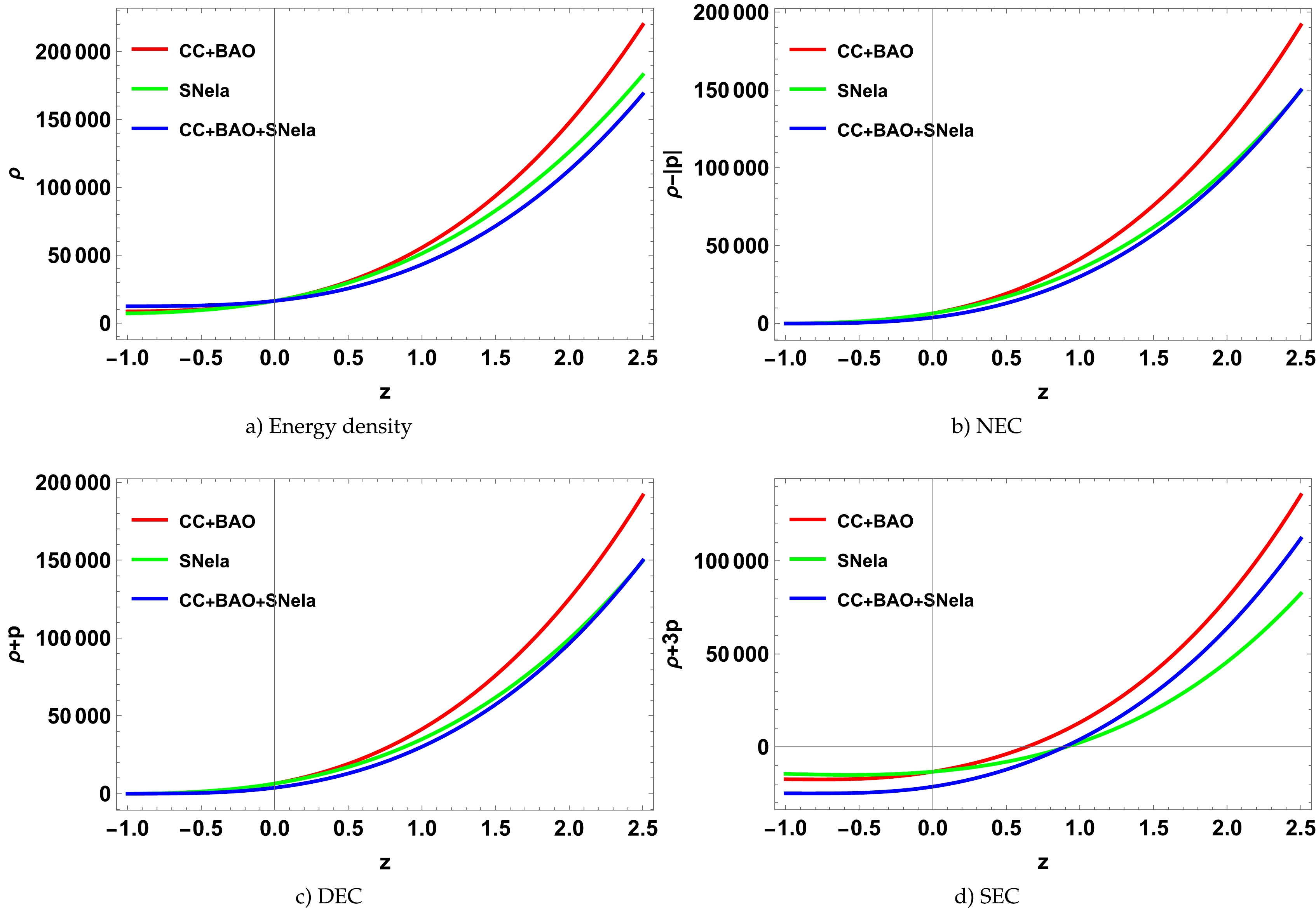
Figure 5. (color online) Profile of (a) the energy density and (b)-(d) different energy conditions for the given model corresponding to the values of the parameters constrained by the CC, BAO, and SNeIa datasets
-
The
$ Om(z) $ diagnostic is a valuable tool for distinguishing between various cosmological or dark energy (DE) models from the ΛCDM model. It was first introduced by Sahni et al. in 2008 [49] and has since been studied extensively by many researchers for the said purpose.$ Om(z) $ is a function that relates the density of matter in the universe to the observed Hubble parameter, which is a measure of how quickly the universe is expanding. If the value of$ Om(z) $ is constant at any redshift, it suggests that DE behaves like a cosmological constant. On the other hand, if$ Om(z) $ varies with redshift, it indicates that the DE is dynamic and takes different forms at different times. Moreover, the slope of$ Om(z) $ can be used to distinguish between two different types of dynamic DE models: quintessence and phantom, where a positive slope of$ Om(z) $ would indicate a phantom phase, while a negative slope would indicate a quintessence phase. Overall, the$ Om(z) $ diagnostic is a powerful tool for studying various cosmological or DE models and provides important insights into the nature of the universe's expansion.In a universe with flat spatial geometry, the Om(z) diagnostic can be expressed as
$ Om(z)=\frac{E^2(z)-1}{(1+z)^3-1}, $

(23) where
$ E(z)=H(z)/H_0 $ . For our model, Eq. (9) together with Eq. (23) gives us an Om diagnostic parameter of$ Om(z)=\frac{((a+z)^4+b)^{(3/4)}-(a^4+b)^{(3/4)}}{(a^4+b)^{(3/4)}(-1+(1+z)^3)}. $

(24) We have plotted the evolution of
$ Om(z) $ with respect to z in Fig. 6, using the constrained parameters of the model obtained from the datasets. After analyzing the CC+ BAO, SNEIa and CC+BAO+SNeIa datasets, the parameters a and b have been constrained, and as a result,$ Om(z) $ displays a negative slope, which suggests the presence of the quintessence epoch. Furthermore, it is evident that our model differs from the ΛCDM model.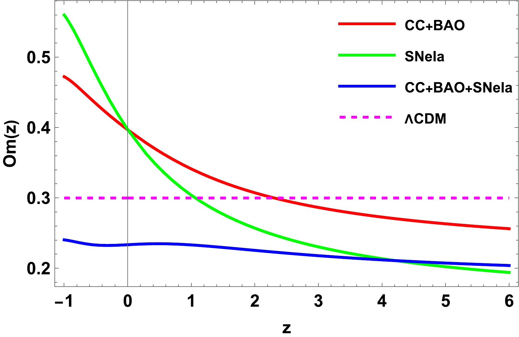
Figure 6. (color online) The behavior of the
$ Om(z) $ diagnostic vs. redshift$ z. $ -
Numerous scientific investigations of researchers across the globe suggest the possible evolution of the cosmos. Recent observational achievements have stimulated investigations beyond standard cosmological models. In this direction, the parametric reconstruction of cosmological entities works reasonably well. The present study explored the cosmological scenario with a newly parameterized DP. The DP is vital in describing the present epoch of the universe by explaining how the Hubble parameter evolves. The DP presented in this paper is capable of explaining several physical phenomena. For instance, the second law of thermodynamics is satisfied by a universe with the DP model (8), which can describe the entropy of the universe. The model consists of two free parameters, which have to be constrained to support the theoretical as well as practical circumstances. For this purpose, we adopted a statistical bayesian inference approach with MCMC formalism. Here, we used 31 CC samples, 26 BAO samples, and 1701 Pantheon+ samples (includeing data from 18 SNeIa surveys along with SH0ES) as observed data points. The best fits (see Table 1) obtained from this procedure are used to analyze the kinematic behavior of the universe. The present Hubble value
$ H_0 $ describes the current expansion rate of the cosmos. Thus, in this work, we constrained$ H_0 $ along with the model parameters. Interestingly, the values obtained for the Hubble constant are consistent with observations. The results of the cosmological quantities for the statistically estimated values of model parameters are presented in Table 2. Here,$ z_t $ explains the transition of the universe from the phase of deceleration to acceleration. For redshifts lower than$ z_t $ , there is a violation of the SEC, confirming the accelerated expansion.Dataset $ q_0 $ 

$ \omega_0 $ 

$ z_t $ 

$ 1\sigma $ 

$ -0.405^{+0.762}_{-0.615} $ 

$ -0.603^{+0.508}_{-0.410} $ 

$ 0.636^{+0.214}_{-0.191} $ 

$\rm CC+BAO$ 

$ 2\sigma $ 

$ -0.405^{+0.817}_{-0.628} $ 

$ -0.603^{+0.545}_{-0.418} $ 

$ 0.636^{+0.355}_{-0.493} $ 

$ 3\sigma $ 

$ -0.405^{+0.854}_{-0.662} $ 

$ -0.603^{+0.569}_{-0.441} $ 

$ 0.636^{+0.421}_{-0.606} $ 

$ 1\sigma $ 

$ -0.404^{+0.046}_{-0.131} $ 

$ -0.603^{+0.031}_{-0.087} $ 

$ 0.906^{+0.559}_{-0.304} $ 

SNeIa $ 2\sigma $ 

$ -0.404^{+0.142}_{-0.310} $ 

$ -0.603^{+0.095}_{-0.207} $ 

$ 0.906^{+0.891}_{-0.550} $ 

$ 3\sigma $ 

$ -0.404^{+0.190}_{-0.410} $ 

$ -0.603^{+0.127}_{-0.274} $ 

$ 0.906^{+1.005}_{-0.632} $ 

$ 1\sigma $ 

$ -0.649^{+0.062}_{-0.053} $ 

$ -0.766^{+0.041}_{-0.035} $ 

$ 0.894^{+0.048}_{-0.049} $ 

CC+BAO+SNeIa $ 2\sigma $ 

$ -0.649^{+0.097}_{-0.107} $ 

$ -0.766^{+0.077}_{-0.072} $ 

$ 0.894^{+0.114}_{-0.086} $ 

$ 3\sigma $ 

$ -0.649^{+0.116}_{-0.135} $ 

$ -0.766^{+0.064}_{-0.090} $ 

$ 0.894^{+0.116}_{-0.102} $ 

Table 2. Summary of the results for DP and effective EoS obtained from constrained values of model parameter with
$ 1\sigma $ -$ 3\sigma $ errorsThe present value of the EoS parameter obtained from different datasets predicts the quintessence behavior of the universe, and the Om profile (Fig. 1) supports this inference. Further, from Fig. 4(b), 4(d), and 4(f) we can see that in the high redshift region, ω approaches zero for all three datasets, meaning the universe is matter-dominated in the early time.
Finally, with the observationally consistent model defined in this article, one can interpret the late-time acceleration of the universe as well as the early-time structure formation. Furthermore, it predicts thermodynamic equilibrium in the long run.
In our future work, we intend to construct parametric models for various cosmological models to investigate the behavior of the universe from a different perspectibe. Moreover, a non-parametric methodology might also be adopted for reconstructing the universe.
-
There are no new data associated with this article.
-
The authors acknowledge DST, New Delhi, India, for its financial support for research facilities under DST-FIST-2019.
-
z $H(z)$ 

${\rm Ref.}$ 

z $H(z)$ 

${\rm Ref.}$ 

z $H(z)$ 

${\rm Ref.}$ 

z $H(z)$ 

${\rm Ref.}$ 

$0.07$ 

$69\pm19.6$ 

[26] $0.09$ 

$69\pm12$ 

[24] $0.12$ 

$68.6\pm26.2$ 

[26] $0.17$ 

$83\pm8$ 

[24] $0.1791$ 

$75\pm4$ 

[25] $0.1993$ 

$75\pm5$ 

[25] $0.2$ 

$72.9\pm29.6$ 

[26] $0.27$ 

$77\pm14$ 

[24] $0.28$ 

$88.8\pm36.6$ 

[26] $0.3519$ 

$83\pm14$ 

[25] $0.3802$ 

$83\pm13.5$ 

[28] $0.4$ 

$95\pm17$ 

[24] $0.4004$ 

$77\pm10.2$ 

[28] $0.4247$ 

$87.1\pm11.2$ 

[28] $0.4497$ 

$87.1\pm11.2$ 

[28] $0.47$ 

$89\pm34$ 

[50] $0.4783$ 

$80.9\pm9$ 

[28] $0.48$ 

$97\pm62$ 

[24] $0.5929$ 

$104\pm13$ 

[25] $0.6797$ 

$92\pm8$ 

[25] $0.7812$ 

$105\pm12$ 

[25] $0.8754$ 

$125\pm17$ 

[25] $0.88$ 

$90\pm40$ 

[24] $0.9$ 

$117\pm23$ 

[24] $1.037$ 

$154\pm20$ 

[25] $1.3$ 

$168\pm17$ 

[25] $1.363$ 

$160\pm33.6$ 

[27] $1.43$ 

$177\pm18$ 

[24] $1.53$ 

$140\pm14$ 

[24] $1.75$ 

$202\pm40$ 

[24] $1.965$ 

$186.5\pm50.4$ 

[27] Table A1. CC data used for analysis.
z $H(z)$ 

${\rm Ref.}$ 

z $H(z)$ 

${\rm Ref.}$ 

z $H(z)$ 

${\rm Ref.}$ 

z $H(z)$ 

${\rm Ref.}$ 

$0.24$ 

$79.69\pm2.99$ 

[30] $0.3$ 

$81.7\pm6.22$ 

[35] $0.31$ 

$78.18\pm4.74$ 

[39] $0.34$ 

$83.8\pm3.66$ 

[30] $0.35$ 

$82.7\pm9.1$ 

[33] $0.36$ 

$79.94\pm3.38$ 

[39] $0.38$ 

$81.5\pm1.9$ 

[40] $0.4$ 

$82.04\pm2.03$ 

[39] $0.43$ 

$86.45\pm3.97$ 

[30] $0.44$ 

$84.81\pm1.83$ 

[31] $0.44$ 

$82.6\pm7.8$ 

[39] $0.48$ 

$87.79\pm2.03$ 

[31] $0.51$ 

$90.4\pm1.9$ 

[40] $0.52$ 

$94.35\pm2.64$ 

[39] $0.56$ 

$93.34\pm2.3$ 

[39] $0.57$ 

$87.6\pm7.8$ 

[32] $0.57$ 

$96.8\pm3.4$ 

[36] $0.59$ 

$98.48\pm3.18$ 

[39] $0.6$ 

$87.9\pm6.1$ 

[31] $0.61$ 

$97.3\pm2.1$ 

[40] $0.64$ 

$98.82\pm2.98$ 

[39] $0.73$ 

$97.3\pm7.0$ 

[31] $2.3$ 

$224\pm8.6$ 

[34] $2.33$ 

$244\pm8$ 

[38] $2.34$ 

$222\pm8.5$ 

[29] $2.36$ 

$226\pm9.3$ 

[37] Table A2. BAO data used for analysis.
The observational data used for analysis in the present paper are provided in Tables A1 and A2.
Observational insights into the accelerating universe through reconstruction of the deceleration parameter
- Received Date: 2023-05-16
- Available Online: 2023-08-15
Abstract: Recent developments in the exploration of the universe suggest that it is in an accelerated phase of expansion. Accordingly, our study aims to probe the current scenario of the universe with the aid of the reconstruction technique. The primary factor that describes cosmic evolution is the deceleration parameter. Here, we provide a physically plausible, newly defined model-independent parametric form of the deceleration parameter. Further, we constrain the free parameters through statistical MCMC analysis for different datasets, including the most recent Pantheon+. With the statistically obtained results, we analyze the dynamics of the model through the phase transition, EoS parameter, and energy conditions. Also, we make use of the tool Om diagnostic to test our model.


 DownLoad: