


 Abstract
 HTML
HTML Reference
 Related
 PDF
PDF


-
Two dimensional JT gravity [1−3] is a model of 2D dilaton gravity that admits AdS
$ _{2} $ holography [4]; it is also the simplest nontrivial theory of gravity. In recent years, JT gravity has provided a simple and meaningful toy model for the study of the black hole information loss problem. In particular, it has been able to describe the Page curve of black hole entropy, which is a key step toward solving the black hole information paradox [5−7]. All these works suggest that after the Page time, there is a configuration in which the entanglement wedge of Hawking radiation includes an island inside the black hole interior, and the island configuration is the key to reproducing the Page curve. Therefore, verifying the validity of the island configurationis of great significance. This has motivated several recent proposals to show the existence of the island by proposing ways to extract information from the island to the radiation [8−11]. One of them is achieved by making use of the modular Hamiltonian and modular flow in entanglement wedge reconstruction and the equivalence between the boundary and bulk modular flow [12]. As a concrete example, extremal black holes with modular flow in JT gravity were considered coupled to baths; it is claimed that the explicit information extraction process can be observed in the case where the bulk conformal fields contain free massless fermion fields [12].While the proposal in [12] shows a promising way to extract information from the island configuration in JT gravity, the details of this process have not been fully specified in the literature. In particular, the modular flow of the free massless fermion field considered in [12] is in two dimensional Minkowski spacetime. More details are needed regarding how to apply this flow to conformally flat spacetime. Therefore, in this paper, we aim to fill this gap in the literature by providing detailed calculations of the entanglement entropy for massless fermion fields with the help of the resolvent technique. Our goal is to provide a clear and comprehensive understanding of the proposed method and its implications for the black hole information paradox.
This paper is organized as follows. In Sec. II, we obtain the equations of motion in the background of JT gravity coupled to primary fermion fields and find the particular solution of the wave function outside the extremal black hole horizon, and we also solve for the dilaton in JT gravity. In Sec. III, we calculate the two point correlators of primary fermion fields under Weyl transformations by the CFT method. In Sec. IV, we review the standard resolvent technique to derive the entanglement entropy in n disjoint intervals for a massless Dirac field in two dimensional vacuum Minkowski spacetime [13, 14]. Accordingly, we redefine the fields in terms of the conformal factor as fermion fields and use the resolvent technique as described in two dimensional vacuum Minkowski spacetime to derive the renormalized entanglement entropy for massless Dirac fields in JT gravity.
-
The JT gravity model consists of 2D gravity coupled to a scalar ϕ called the dilaton, with a classical bulk term action in the Lorentzian signature on an asymptotically AdS spacetime,
$ S_{\text{JT}}=\frac{1}{16\pi G_N}\int {\rm d}^{2}x\sqrt{-g}\left(\phi R+2\phi-2\phi_0\right), $

(1) where R is the Ricci scalar and we have set the AdS
$ _{2} $ length$l_{\rm AdS} = 1$ . The JT gravity action originates from a dimensional reduction of the four dimensional near extremal magnetic charged black hole [15−17], and the two-dimensional JT model is obtained by reduction of the spherically symmetric metric,$ {\rm d}s^{2}_4=g_{\mu\nu}(t,r){\rm d}x^{\mu}{\rm d}x^{\nu}+\phi(t,r){\rm d}\Omega^{2}_2,$

(2) where
$ g_{\mu\nu} $ is the 2D part with coordinates$ (t,r) $ the dilaton ϕ plays the role of the radius of the 2-sphere that we want to reduce, and$ \phi_0 $ is a constant proportional to the extremal entropy of the higher-dimensional black hole geometry.In this paper, we consider the coupling of a massless Dirac field
$ \Psi(x) $ to JT gravity. The massless Dirac field, also called the primary field, satisfies conformal invariance under conformal transformations in the CFT method. The action of primary fermion fields in 2D curved spacetime is [18−22]:$ S_{\text{D}}=\frac{\rm i}{2}\int {\rm d}^{2}x\sqrt{-g} \overline{\Psi}\left(\overline{\gamma}^{\mu}\overleftrightarrow{D_{\mu}} \Psi\right), $

(3) where
$ \overrightarrow{D_{\mu}}=\overrightarrow{\partial_{\mu}}+\Gamma_{\mu}=\overrightarrow{\partial_{\mu}}+\frac{1}{8}\eta_{ac}{{\omega_{\mu}}^{c}}_{b}[\gamma^{a},\gamma^{b}] $ is the spinor covariant derivative, and the spin connection is$ {{\omega_{\mu}}^{c}}_{b}= -{e_{b}}^{\nu}\left(\partial_{\mu}{e^{c}}_{\nu}-\Gamma_{\mu\nu}^{\lambda} {e^{c}}_{\lambda}\right) $ 1 . Note that in Eq. (3),${\rm i}\overline{\Psi}\left(\overline{\gamma}^{\mu}\overrightarrow{D_{\mu}}\Psi\right)$ is not real, so we should choose$\dfrac{\rm i}{2}\overline{\Psi}\left(\overline{\gamma}^{\mu}\overleftrightarrow{D_{\mu}}\Psi\right)$ as the Dirac Lagrangian, where$ \overleftarrow{D_{\mu}}=\overleftarrow{\partial_{\mu}}-\Gamma_{\mu}= \overleftarrow{\partial_{\mu}}- \dfrac{1}{8}\eta_{ac}{{\omega_{\mu}}^{c}}_{b}[\gamma^{a},\gamma^{b}] $ operates on$ \overline{\Psi} $ , and$ \overleftarrow{D_{\mu}} $ is different from$ \overrightarrow{D_{\mu}} $ .We adopt the metric signature
$ (-,+) $ and the anticommutator of the Dirac gamma metric is$ \{\gamma^{a},\gamma^{b}\}=2\eta^{ab}\mathit{\pmb{1}} $ . The Dirac gamma matrices have this property:$ (\gamma^{0})^{2}=-\mathit{\pmb{1}} $ and$ (\gamma^{1})^{2}=\mathit{\pmb{1}} $ ; we choose$ \begin{array}{*{20}{l}} \gamma^{0}=\left(\begin{array}{cc}0 & 1\\-1 & 0\end{array}\right), \quad\gamma^{1}=\left(\begin{array}{cc}0 & 1 \\1 & 0\end{array}\right). \end{array} $

(4) The Dirac adjoint in Eq. (3) is defined as
$ \overline{\Psi}=\Psi^{\dagger}\gamma^{0} $ , and$ \overline{\gamma}^{\mu}={e_{a}}^{\mu}\gamma^{a} $ , where$ {e_{a}}^{\mu} $ is the vierbein.We define α as the strength of the coupling between the massless Dirac field and JT gravity, and we also define
$ \kappa^{2}\equiv 8\pi G_N $ , whereupon the total action functional is$ \begin{aligned}[b] S=&S_{\text{JT}}+\alpha S_{\text{D}}=\int {\rm d}^{2}x\sqrt{-g}\Bigg[\frac{1}{2\kappa^{2}}\left(\phi R+2\phi-2\phi_0\right)\\&+\frac{{\rm i}\alpha}{2}\overline{\Psi}\left(\overline{\gamma}^{\mu}\overleftrightarrow{D_{\mu}}\Psi\right)\Bigg]. \end{aligned} $

(5) By varying the total action (5) with respect to the metric field, we obtain the classical equations of motion (see Appendix A):
$ g_{\mu \nu}(\phi-\phi_0)+\nabla_{\mu}\nabla_{\nu}\phi-g_{\mu \nu}\square\phi=\frac{{\rm i}\alpha\kappa^{2}}{8}\overline{\Psi}\Big(\gamma_{\nu}\overleftrightarrow{D_{\mu}}+\gamma_{\mu}\overleftrightarrow{D_{\nu}}\Big)\Psi, $

(6) where
$ \gamma_{\nu} $ is defined as$ \gamma_{\nu}=(g_{\mu \nu}{e_{a}}^{\mu})\gamma^{a}=g_{\mu \nu}\overline{\gamma}^{\mu} $ , and${\rm i}\overline{\Psi}\left(\gamma_{\mu}\overleftrightarrow{D_{\nu}}\Psi\right)$ is defined as${\rm i}\overline{\Psi}\left(\gamma_{\mu}\overleftrightarrow{D_{\nu}}\Psi\right)={\rm i}\overline{\Psi}\gamma_{\mu}\overrightarrow{D_{\nu}}\Psi+ \left({\rm i}\overline{\Psi}\gamma_{\mu}\overrightarrow{D_{\nu}}\Psi\right)^{\dagger}$ , with$\left({\rm i}\overline{\Psi}\gamma_{\mu}\overrightarrow{D_{\nu}}\Psi\right)^{\dagger}=-{\rm i}\left(\overline{\Psi}\overleftarrow{D_{\nu}}\right)\gamma_{\mu}\Psi$ . -
In a generic conformal coordinate system
$ x^{\pm} $ , the metric in two dimensional gravity is given by$ \begin{array}{*{20}{l}} {\rm d}s^2=-{\rm e}^{2\rho(x^+,x^-)}{\rm d}x^+ {\rm d}x^-. \end{array} $

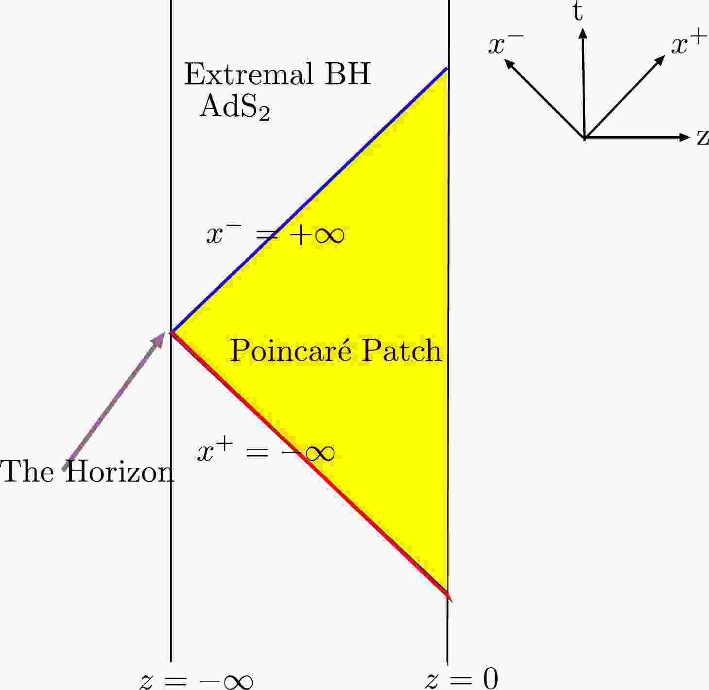
(7) In this paper we consider a zero temperature black hole in the two-dimensional Jackiw-Teitelboim gravity, and we can use the Poincaré coordinates
$ x^{\pm} = t \pm z $ to describe the extremal black hole (see Fig. 1 for more details). The metric in the Poincaré patch is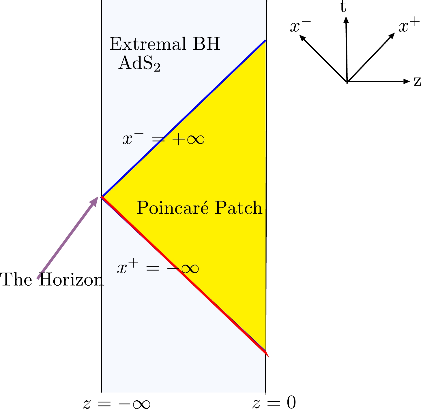
Figure 1. (color online) The Penrose diagram for the extreme black hole in JT gravity. The yellow region is the Poincaré patch where the wave function is distributed. The blue null line is the future event horizon and the red null line is the past event horizon. Here z ranges
$ z \in (-\infty,0] $ , where$ z = -\infty $ is the location of the horizon.$ {\rm d}s^{2}=-\frac{4{\rm d}x^+ {\rm d}x^-}{\left(x^+-x^-\right)^2}=\frac{-{\rm d}t^{2}+{\rm d}z^{2}}{z^{2}} , \; z \leqslant 0. $

(8) The boundary of AdS
$ _{2} $ spacetime is at$ z = 0 $ , the future horizon of the JT extremal black hole is at$ x^{-}=+\infty $ , and the past horizon is at$ x^{+}=-\infty $ .By varying the Dirac action
$ S_{\text{D}} $ with respect to the Dirac field, we obtain the massless Dirac field equation in two dimensional conformally flat spacetime$ \begin{array}{*{20}{l}} {\rm i}\overline{\gamma}^{\mu}{D_{\mu}}\Psi=0. \end{array} $

(9) We can write the 2-component massless Dirac spinor Ψ as
$ \begin{array}{*{20}{l}} \Psi=\left(\begin{array}{cc}\Psi_{1} \\ \Psi_{2}\end{array}\right)=\left(\begin{array}{cc}\psi_{1}+{\rm i}\psi_{2} \\ \psi_{3}+{\rm i}\psi_{4}\end{array}\right). \end{array} $

(10) As any two dimensional spacetime is conformally flat, the massless Dirac field equation in the conformal gauge can be written
2 $ 2\partial_+\Psi_{1}-\frac{\Psi_{1}}{\left(x^+-x^-\right)}=0, \quad -2\partial_-\Psi_{2}-\frac{\Psi_{2}}{\left(x^+-x^-\right)}=0. $

(11) The wave function in JT gravity spacetime must satisfy the following two boundary conditions: The wave function is zero at the AdS
$ _{2} $ spacetime boundary and finite at the past event horizon or the future event horizon of the extreme black hole in JT gravity. Combining the two boundary conditions and Eq. (11), we find a particular solution of the wave function distribution beyond the extremal black hole horizon:$ \begin{aligned}[b] \Psi_{1}(x^+,x^-)=&\frac{1}{\sqrt{x^-}}\left(x^--x^+\right)^{\frac{1}{2}}+{\rm i}\frac{1}{\sqrt{x^-}}\left(x^--x^+\right)^{\frac{1}{2}},\\ \Psi_{2}(x^+,x^-)=&\frac{1}{\sqrt{-x^+}}\left(x^--x^+\right)^{\frac{1}{2}}+{\rm i}\frac{1}{\sqrt{-x^+}}\left(x^--x^+\right)^{\frac{1}{2}}. \end{aligned} $

(12) -
In the conformal gauge, using the general metric in two dimensional gravity in Eq. (7), from Eq. (6) we finally have
3 ,$ \begin{aligned}[b] \text{(1) For\; the\; metric}\ g_{+-}:~& \frac{e^{2\rho}}{2}\left(\phi_0-\phi\right)-\partial_+\partial_-\phi\\=&\frac{{\rm i}\alpha\kappa^{2}}{8} \overline{\Psi}\Big(\gamma_-\overrightarrow{D_+}-\overleftarrow{D_+}\gamma_-\\&+\gamma_+\overrightarrow{D_-}-\overleftarrow{D_-}\gamma_+\Big)\Psi, \end{aligned} $

(13) $ \begin{aligned}[b] \text{(2) For\; the\; metric}\ g_{++}:~ & \partial_+\partial_+\phi-2\partial_+ \rho \partial_+\phi\\=&\frac{{\rm i}\alpha\kappa^{2}}{4}\overline{\Psi}\left(\gamma_+\overrightarrow{D_+}-\overleftarrow{D_+}\gamma_+\right)\Psi, \end{aligned} $

(14) $ \begin{aligned}[b] \text{(3) For\; the\; metric}\ g_{–}:~ &\partial_-\partial_-\phi-2\partial_- \rho \partial_- \phi\\=&\frac{{\rm i}\alpha\kappa^{2}}{4}\overline{\Psi}\left(\gamma_-\overrightarrow{D_-}-\overleftarrow{D_-}\gamma_-\right)\Psi. \end{aligned} $

(15) As the direction of the tetrad can be arbitrarily selected, we choose
${e_{0}}^{+}={e_{0}}^{-}={e_{1}}^{-}=-e^{-\rho}$ and${e_{1}}^{+}=e^{-\rho}$ . We then obtain the expression for the connection$ \Gamma_{\mu} $ and the matrix$ \gamma_{\mu} $ in the conformal gauge:$ \gamma_+=\frac{e^{\rho}}{2}\left(\gamma^0+\gamma^1\right),~~~ \gamma_-=\frac{e^{\rho}}{2}\left(\gamma^0-\gamma^1\right), $

(16) $ \Gamma_+=\frac{\partial_+\rho}{2}\gamma^0\gamma^1,~~~ \Gamma_-=\frac{\partial_-\rho}{2}\gamma^1\gamma^0. $

(17) Next, we substitute the 2-component massless Dirac spinor (10) into the right hand side of Eq. (14), Eq. (15), and Eq. (16). Using Eq. (17) and Eq. (18), we then have
$ \overline{\Psi}\left(\gamma_-\overrightarrow{D_+}-\overleftarrow{D_+}\gamma_-+\gamma_+\overrightarrow{D_-}-\overleftarrow{D_-}\gamma_+\right)\Psi=0, $

(18) $ \overline{\Psi}\left(\gamma_+\overrightarrow{D_+}-\overleftarrow{D_+}\gamma_+\right)\Psi=\frac{e^\rho}{2} \left(-2\Psi_{2}^{\ast}\partial_+\Psi_{2}+2\Psi_{2}\partial_+\Psi_{2}^{\ast}\right)$

(19) $ \overline{\Psi}\left(\gamma_-\overrightarrow{D_-}-\overleftarrow{D_-}\gamma_-\right)\Psi=\frac{e^\rho}{2} \left(-2\Psi_{1}^{\ast}\partial_-\Psi_{1}+2\Psi_{1}\partial_-\Psi_{1}^{\ast}\right) $

(20) Substituting the particular solution of the 2-component massless Dirac spinor (12) back into the right hand side of Eq. (20) and Eq. (21), we find
$ -2\Psi_{2}^{\ast}\partial_+\Psi_{2}+2\Psi_{2}\partial_+\Psi_{2}^{\ast}=0, \; -2\Psi_{1}^{\ast}\partial_-\Psi_{1}+2\Psi_{1}\partial_-\Psi_{1}^{\ast}=0. $

(21) Finally, the equation of motion for the dilaton becomes
$ \begin{aligned}[b] \frac{2}{\left(x^+-x^-\right)^{2}}\left(\phi_0-\phi\right)-\partial_+\partial_-\phi=&0,\\ \frac{2}{\left(x^+-x^-\right)}\partial_+\left(\frac{\left(x^+-x^-\right)^{2}}{4}\partial_+\phi\right)=&0,\\ \frac{2}{\left(x^+-x^-\right)}\partial_-\left(\frac{\left(x^+-x^-\right)^{2}}{4}\partial_-\phi\right)=&0. \end{aligned} $

(22) We can solve the equation for the dilaton
$ \phi=\phi_0+\frac{a+b\left(x^++x^-\right)+cx^+x^-}{\left(x^+-x^-\right)}, $

(23) where a, b, and c are constants that determine the dilaton of JT gravity.
In particular, the dilaton diverges at the conformal boundary, and the location of this physical boundary is imposed by the boundary condition [23]:
$ g_{uu}\mid_{bdy}=\frac{1}{\varepsilon^2}, \quad \phi=\phi_{b}=\frac{\phi_{r}}{\varepsilon}+\phi_0, $

(24) where u is the physical boundary time, with ε the UV cutoff.
The metric in JT gravity has
$ SL(2,R) $ isometry. For the extreme black hole in JT gravity, under the$ SL(2,R) $ transformation the dilaton profiles can be recast as$ \phi=\phi_0+\frac{2\phi_{r}}{\left(x^+-x^-\right)}. $

(25) -
We consider a free Dirac field in two dimensions. It satisfies the Dirac equation and the canonical anticommutation relations :
$ \left({\rm i}\gamma^{\mu}\partial_{\mu}-m\right)\Psi=0, \quad \{\Psi_{\alpha}(\vec{x}),\Psi_{\beta}^{\dagger}(\vec{y})\}=\delta_{\alpha\beta}\delta(\vec{x}-\vec{y}), $

(26) where x and y lie on the Cauchy surface with t = constant. The two point field correlator in two dimensional Minkowski spacetime is
4 :$ C(\vec{x},\vec{y})=\langle0|\Psi(\vec{x})\Psi^{\dagger}(\vec{y})|0\rangle=\int\frac{{\rm d}p}{2\pi}\frac{\left(p_{\mu}\gamma^{\mu}+m\right)}{2\sqrt{p^2+m^2}}\gamma^{0}{\rm e}^{-{\rm i}p\cdot\left(x-y\right)}. $

(27) The integral of the two point field correlator in Eq. (28) is [13]:
$ \begin{aligned}[b] C(x,y)=&\frac{1}{2}\delta\left(x-y\right) {1}+\frac{m}{2\pi}K_{0}\left(m|x-y|\right)\gamma^{0}\\&+\frac{{\rm i} m}{2\pi}K_{1}\left(m\left(x-y\right)\right)\gamma^{0}\gamma^{1}, \end{aligned} $

(28) where
$ K_{n}(x) $ is the standard modified Bessel function; in the massless limit this gives the two point correlator for the primary fermion field in two dimensional flat spacetime:$ C(x,y)=\frac{1}{2}\delta\left(x-y\right) {1}+\frac{\rm i}{2\pi}\frac{1}{\left(x-y\right)}\gamma^{0}\gamma^{1}. $

(29) -
In general, the metric in 2D conformally flat spacetime is:
$ {\rm d}s^2=-{\rm e}^{2\rho(x^+,x^-)}{\rm d}x^+ {\rm d}x^-=-\Omega^{-2}(x^+,x^-){\rm d}x^+ {\rm d}x^-, $

(30) where
$\Omega={\rm e}^{-\rho}$ is the conformal factor. Two dimensional JT gravity is locally AdS$ _{2} $ spacetime with the conformal factor$ \Omega=\left(x^{+}-x^{-}\right)/2 $ .In the CFT method, the two point correlation function for primary operators on a curved manifold with Weyl rescaled metric
$ \Omega^{-2}g $ in terms of those with metric g satisfies the following transformation relation under Weyl transformations [5, 24]:$ \begin{aligned}[b] & \langle\Phi\left(x_{1}, \bar{x}_{1}\right) \tilde{\Phi}\left(x_{2}, \bar{x}_{2}\right)\rangle_{\Omega^{-2}g}\\=&\Omega\left(x_{1}, \bar{x}_{1}\right)^{\Delta}\Omega\left(x_{2},\bar{x}_{2}\right)^{\Delta}\langle\Phi\left(x_{1},\bar{x}_{1}\right)\tilde{\Phi}\left(x_{2}, \bar{x}_{2}\right)\rangle_{g}, \end{aligned} $

(31) where Δ is the scale dimension for the twist field and
$ \langle\Phi\left(x_{1},\bar{x}_{1}\right)\tilde{\Phi}\left(x_{2}\bar{x}_{2}\right)\rangle_{g} $ is the two point correlation function for primary operators in two dimensional flat spacetime.The free massless fermion field is also the primary field with the scale dimension
$ \Delta = 1/2 $ . Combining Eq. (30) and Eq. (32), we obtain the two point correlators of the primary fermion fields$ C(x,y)_{\Omega^{-2}g} $ in JT gravity when Weyl transformed from${\rm d}s^2 = -{\rm d}x^+ {\rm d}x^-$ to${\rm d}s^2 = -\Omega^{-2}(x^+, x^-){\rm d}x^+ {\rm d}x^-$ :$ \begin{aligned}[b] C(x,y)_{g}=&\langle\Phi\left(x,\bar{x}\right)\tilde{\Phi}\left(y,\bar{y}\right)\rangle_{g}=\frac{1}{2}\delta\left(x-y\right) {1}\\&+\frac{\rm \rm i}{2\pi}\frac{1}{\left(x-y\right)}\gamma^{0}\gamma^{1}\\ \Longrightarrow C(x,y)_{\Omega^{-2}g}=&\langle\Phi\left(x, \bar{x}\right) \tilde{\Phi}\left(y, \bar{y}\right)\rangle_{\Omega^{-2}g}=\frac{\left(xy\right)^{\frac{1}{2}}}{2}\delta\left(x-y\right) {1}\\&+\frac{\rm i}{2\pi}\frac{\left(xy\right)^{\frac{1}{2}}}{\left(x-y\right)}\gamma^{0}\gamma^{1}. \end{aligned} $

(32) -
The entanglement entropy (von Neumann entropy) provides us with a convenient way to measure the degree of entanglement between two quantum systems in QFT. We choose the total quantum system as a pure quantum state with the density matrix
$ \rho=|\Psi\rangle\langle\Psi| $ . The reduced density matrix for the subsystem A is$ \rho_{A}=Tr_{B}|\Psi\rangle\langle\Psi| $ , which is obtained by taking a partial trace over the subsystem B of the total density matrix (see Fig. 2). The entanglement entropy for the subsystem A is the corresponding von Neumann entropy: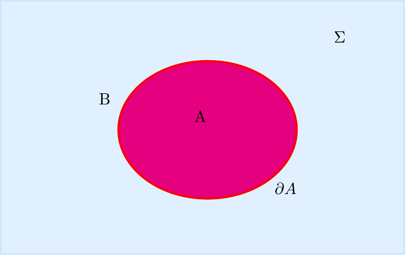
Figure 2. (color online) A continuum QFT has been spatially divided into two components on a Cauchy slice Σ. Region B is the complement of region A, and the red curve
$ \partial A $ is the entangling surface, which is a spacetime codimension-2 surface.$ S_{A}=-Tr\left(\rho_{A}\ln\rho_{A}\right). $

(33) For the 1+1 dimensional quantum system at criticality, the continuum limit is a conformal field theory with central charge c. The renormalized entanglement entropy of a single interval in vacuum state in flat spacetime can be calculated by the Cardy formula [25, 26]:
$ S=\frac{c}{3}\log\ell, $

(34) where
$ \ell $ is the length of the interval on the line in vacuum. After Weyl transformation from${\rm d}s^2 = -{\rm d}x^+ {\rm d}x^-$ to${\rm d}s^2 = -\Omega^{-2}(x^+,x^-){\rm d}x^+ {\rm d}x^-$ , the entanglement entropy in 2D conformally flat spacetime is transformed as [5, 27]:$ S_{\Omega^{-2} g}=S_{g}-\frac{c}{6}\sum\limits_{\rm endpoints}\log(\Omega)=S_{g}+\frac{c}{6}\sum\limits_{\rm endpoints}\log( e^{\rho}). $

(35) The entanglement entropy is related to the reduced density matrix of the region V; hence, the problem of finding an explicit expression for the local density matrix
$ \rho_{V} $ is equivalent to solving the resolvent of the two point correlators$ C_{V} $ in the massless case. Resolvent is a standard technique in complex analysis; the use of the resolvent technique for free massless fermions was first introduced in [13] to study the entanglement entropy in vacuum on the plane, and subsequently for the entanglement entropy of a chiral fermion on the torus [28−30]. In this section we first review the derivation of the entanglement entropy for a massless Dirac field in two dimensional vacuum Minkowski spacetime in terms of the resolvent technique, and we then obtain the entanglement entropy of a single interval for a massless Dirac field in 2D conformally flat JT gravity by redefining the field in terms of the conformal factor as the Fermion field. -
The two point function
$ C_{V} $ is related to the reduced density matrix of the region V by the condition:$ C_{V}(x,y)=\langle\Psi(x)\Psi^{\dagger}(y)\rangle=Tr\left(\rho_{V}\Psi(x)\Psi^{\dagger}(y)\right). $

(36) The expression for the entanglement entropy of the region V can then be given by a propagator trace formula (see Appendix D) [13, 14, 31]:
$ S_{V}=-Tr[\left(1-C_{V}\right)\log\left(1-C_{V}\right)+C_{V}\log C_{V}]. $

(37) The resolvent of the two point function
$ C_{V} $ is defined as:$ R_{V}(\xi):=\left(C_{V}+\xi-1/2\right)^{-1}. $

(38) Combining the the expression for the resolvent (39), the entanglement entropy can be rewritten as:
$ S_{V}=-Tr\int^{+\infty}_{1/2}{\rm d}\xi\left[(\xi-1/2)[R(\xi)-R(-\xi)]-\frac{2\xi}{\xi+1/2}\right]. $

(39) In Eq. (39), the inverse of an operator for the propagator is understood in the sense of a kernel that satisfies the following equation:
$ \begin{aligned}[b] & \int_{V}{\rm d}z R_{V}(\xi;x,z)R_{V}^{-1}(\xi;z,y)=\delta\left(x-y\right)\\=&\int_{V}{\rm d}z R_{V}(\xi;x,z)[C(z,y)+\left(\xi-1/2\right)\delta(z,y)]. \end{aligned} $

(40) Substituting (30) into (41) yields a singular integral equation [32]:
$ \xi R_{V}(x,y)-\frac{\rm i}{2\pi }\int_{V}\frac{R_{V}(x,z)}{z-y}{\rm d}z=\delta\left(x-y\right). $

(41) Fortunately, we can solve the resolvent for this integral operator inside a region formed by n disjoint intervals
$ (u_{i},v_{i}) $ by the Plemelj formulae [32] in the theory of singular integral equations (see Appendix B). The resolvent of the two point function$ C_{V} $ (see Appendix C):$ R_{V}(\xi) =\left(\xi^2-1/4 \right)^{-1} \left(\xi\,\delta(x-y)\,+\frac{\rm i }{2\pi} \frac{{\rm e}^{ -\frac{\rm i}{2\pi} \log\left(\frac{\xi-1/2}{\xi+1/2}\right)\, \left(z(x)-z(y)\right) }}{x-y} \right), $

(42) where the function
$ z(x) $ is$ z(x)=\log\left(-\frac{\prod_{i=1}^n (x-u_i)}{\prod_{i=1}^n (x-v_i)}\right). $

(43) Substituting (43) into (40), we have
$ \begin{aligned}[b] S_{V}=&-\frac{2}{\pi}\int^\infty_{1/2} {\rm d}\xi\, \int_V {\rm d}x\, \lim\limits_{y\rightarrow x} \\&\times \frac{\sin\left[ \dfrac{1}{2\pi} \log\left(\dfrac{\xi-1/2}{\xi+1/2}\right)\, \left(z(x)-z(y)\right) \right]}{(\xi+1/2)\,(x-y)}\,.\end{aligned} $

(44) Integrating over ξ first, we obtain the entanglement entropy in n disjoint intervals for a massless Dirac field in two dimensional vacuum Minkowski spacetime:
$ \begin{aligned}[b] S_{V}=&2\int_V {\rm d}x\, \lim_{y\rightarrow x} \frac{\frac{z(x)-z(y)}{2}\coth\left(\left(z(x)-z(y)\right)/2\right)-1}{(x-y)\left(z(x)-z(y)\right)}\\=&\frac{1}{6}\int_V {\rm d}x\,\sum\limits_{i=1}^n \left(\frac{1}{x-u_i}-\frac{1}{x-v_i}\right)\\ =&\frac{1}{3} \Big( \sum\limits_{i,j}\log|v_i-u_i|-\sum\limits_{i<j} \log|u_i-u_j| \\&-\sum\limits_{i<j} \log|v_i-v_j|-n \log \epsilon \Big)\,, \end{aligned} $

(45) where
$ \epsilon $ is a distance cutoff introduced in the last integration, and the Virasoro central charge of the primary fermion field is$ c=1 $ . For a single interval in 2D vacuum flat spacetime on the plane, we verify the Cardy formula for the renormalized entanglement entropy$ S=\dfrac{c}{3}\log\ell $ . -
In this subsection, we apply the resolvent technique to 2D conformally flat spacetime. We begin by redefining the field in terms of the conformal factor as the Fermion field
5 . Let us consider the rescaling field, which is given by:$ \begin{array}{*{20}{l}} \hat\Psi(\vec{x})=\Omega^\Delta(\vec{x}) \Psi(\vec{x})=\Omega^\frac{1}{2}(\vec{x}) \Psi(\vec{x}), \end{array} $

(46) Using this rescaling field, we can use the same approach as described in the previous subsection and obtain the same results as in Eq. (46). After performing the calculations using the original field
$ \Psi(\vec{x}) $ , one finally finds$ \begin{aligned}[b] S_{V}=&\frac{1}{3} \left( \sum\limits_{i,j}\log|\frac{v_i-u_i}{(u_iv_i)^{1/2}}|-\sum\limits_{i<j} \log|\frac{u_i-u_j}{(u_iu_j)^{1/2}}| \right.\\&\left.-\sum\limits_{i<j} \log|\frac{v_i-v_j}{(v_iv_j)^{1/2}}|-n \log \epsilon \right)\,, \end{aligned} $

(47) The renormalized entanglement entropy for a massless Dirac field of a single interval in JT gravity is
6 :$ S=\frac{1}{6}\log\frac{\ell^2}{\Omega_{A}\Omega_{B}}=\frac{1}{3}\log\frac{|x-y|}{(xy)^{\frac{1}{2}}}, $

(48) where the Virasoro central charge of the massless Dirac field is
$ c = 1 $ . -
In this paper we obtain the particular solution of the wave function outside the extremal black hole horizon in JT gravity, which is very important for research on the extraction of extremal black hole information with modular flow in JT gravity. The specific expression for the modular flow of 2D free massless fermions depends on the wave function. Other papers have derived the modular flow formula for 2D free massless fermions, but did not report the specific expression for the wave function [12, 28, 33, 34].
In CFT
$ _2 $ methods, a convenient way to compute entropies of intervals is by using the replica trick to compute the Rényi entropy for integer index n:$ S_{n}(V)=\frac{1}{1-n}\log Tr\rho^n_{V}. $

(49) Taking the limit
$ n\rightarrow1 $ , we can derive the entanglement entropy of the primary fermion fields [5, 25, 26]. The resolvent technique is a simpler way to derive the entanglement entropy for 2D free massless fermions than the CFT method called the replica trick. In this paper we calculate the two point correlators of primary fermion fields in JT gravity under Weyl transformations and redefine the fields in terms of the conformal factor as the fermion fields, then use the resolvent technique as described in two dimensional vacuum Minkowski spacetime to derive the renormalized entanglement entropy for massless Dirac fields in JT gravity.In this work, we have calculated the wave function and derived the entanglement entropy for the primary fermion fields outside the extremal black hole horizon in JT gravity. We only consider the quantum entanglement between free massless fermions outside the extremal black hole horizon. For the entanglement between free massless fermions inside and outside the horizon, however, we should regard the entirety of spacetime as a total quantum system composed of the extremal black hole and Hawking radiation outside the horizon. The degrees of freedom for the free massless fermions located inside the horizon represent the degrees of freedom of the extremal black hole, and the degrees of freedom for the free massless fermions located outside the horizon represent the degrees of freedom of Hawking radiation particles. In order to calculate the entanglement entropy for the free massless fermions both inside the horizon and outside the horizon, we should consider the entanglement island inside the extremal black hole interior in JT gravity. We may calculate the fine grained entropy of the extremal black hole and Hawking radiation via the semiclassical method called the island rule. We leave the full analysis of this for future work.
-
We thank Hong-An Zeng for helpful discussions on the resolvent of the primary fermion correlator in 2D vacuum Minkowski spacetime.
-
The total action functional for JT gravity coupled to primary fermions is given by Eq. (5), from which we obtain the classical equation of motion by varying the metric of the total action:
$ \frac{\delta S}{\delta g^{\mu\nu}}=0, \; \Longrightarrow -\frac{\delta S_{JT}}{\delta g^{\mu\nu}} = \frac{\alpha\delta S_{D}}{\delta g^{\mu\nu}}. \tag{A1}$

The variation of (3) with respect to the frame vector indices
${e}^{a\mu}$ is [18]:$ \delta S_{D}=\int {\rm d}^2x\frac{\rm i}{4}\sqrt{-g}\overline{\Psi}\left[\gamma_{a}\overleftrightarrow{D_{\mu}}+\gamma_{\mu}{e_{a}}^{\rho}\overleftrightarrow{D_{\rho}}\right]\Psi\delta {e}^{a\mu}, \tag{A2} $

where
$\eta^{ab}{e_b}^{\mu}={\rm e}^{a\mu}$ . We use$ \delta e^{a\mu}=\dfrac{1}{4}{e^a}_{\nu}\delta g^{\mu\nu} $ . By the variation of the metric$ g^{\mu\nu} $ , Eq. (52) can be written:$ \delta S_{D}=\int {\rm d}^2x\frac{\rm i}{16}\sqrt{-g}\overline{\Psi}\left[\gamma_{\nu}\overleftrightarrow{D_{\mu}}+\gamma_{\mu}\overleftrightarrow{D_{\nu}}\right]\Psi\delta g^{\mu\nu}, \tag{A3} $

where we have used the following contractions in (53),
$ \gamma_{a}{e^a}_{\nu}=\gamma_{\nu}, \;{e_a}^{\rho}{e^a}_{\nu}=\delta^{\rho}_{\nu}. \tag{A4} $

For the classical bulk term action of JT gravity (1), using the standard relations [35],
$ \begin{aligned}[b] \delta\sqrt{-g}=&-\frac{1}{2}\sqrt{-g}g_{\mu\nu}\delta g^{\mu\nu}, \;\phi g^{\mu\nu}\delta R_{\mu\nu}\\=&-\left[\left(\nabla_{\mu}\nabla_{\nu}-g_{\mu\nu}\square\right)\phi\right]\delta g^{\mu\nu}. \end{aligned}\tag{A5} $

By varying the metric
$ g^{\mu\nu} $ in 2D spacetime, we obtain:$ \begin{aligned}[b] \delta S_{JT}=&\frac{1}{16\pi G_N}\int {\rm d}^2x\Big[\delta(\sqrt{-g})\left(\phi R+2\phi-2\phi_0\right)\\&+\sqrt{-g}\phi\delta(g^{\mu\nu}R_{\mu\nu})\Big]\\ =&\frac{1}{16\pi G_N}\int {\rm d}^2x\sqrt{-g}\Bigg[-\frac{1}{2}\sqrt{-g}g_{\mu\nu}\delta g^{\mu\nu}\left(\phi R+2\phi-2\phi_0\right)\\&+\sqrt{-g}\phi R_{\mu\nu}\delta g^{\mu\nu}+\sqrt{-g}\phi g^{\mu\nu}\delta R_{\mu\nu}\Bigg]\\ =&\frac{1}{16\pi G_N}\int {\rm d}^2x\sqrt{-g}\Bigg[-\frac{1}{2}\sqrt{-g}g_{\mu\nu}\delta g^{\mu\nu}\left(\phi R+2\phi-2\phi_0\right)\\&+\sqrt{-g}\phi R_{\mu\nu}\delta g^{\mu\nu}+\sqrt{-g}\left[g_{\mu\nu}\square-\nabla_{\mu}\nabla_{\nu}\right]\phi\delta g^{\mu\nu}\Bigg]\\ =&\frac{1}{32\pi G_N}\int {\rm d}^2x\sqrt{-g}\Bigg[2g_{\mu\nu}\left(\phi_0-\phi\right)+2\phi\left(R_{\mu\nu}-\frac{1}{2}g_{\mu\nu}R\right)\\&+2g_{\mu\nu}\square\phi-2\nabla_{\mu}\nabla_{\nu}\phi\Bigg]\delta g^{\mu\nu}. \end{aligned}\tag{A6} $

In 2D gravity, we can easily calculate that the Einstein tensor is zero. In the last term in Eq. (56), we have
$ G_{\mu\nu}=R_{\mu\nu}-\dfrac{1}{2}g_{\mu\nu}R=0 $ . Eq. (56) then becomes$ \begin{aligned}[b] \delta S_{JT}=&\frac{1}{32\pi G_N}\int {\rm d}^2x\sqrt{-g}\Big[2g_{\mu\nu}\left(\phi_0-\phi\right)\\&+2g_{\mu\nu}\square\phi-2\nabla_{\mu}\nabla_{\nu}\phi\Big]\delta g^{\mu\nu}. \end{aligned}\tag{A7} $

Finally, substituting (53) and (57) into (51) yields the classical equation of motion in JT gravity coupled to primary fermion fields:
$ g_{\mu \nu}\left(\phi-\phi_0\right)+\nabla_{\mu}\nabla_{\nu}\phi-g_{\mu \nu}\square\phi=\frac{{\rm i}\alpha\kappa^{2}}{8}\overline{\Psi}\left(\gamma_{\nu}\overleftrightarrow{D_{\mu}}+\gamma_{\mu}\overleftrightarrow{D_{\nu}}\right)\Psi. \tag{A8} $

-
For the entire complex plane (see the Fig. 3), we obtain the integral formula of the function
$ \varphi(t_0) $ using Cauchy's integral formula [32]:
Figure 3. (color online) L is a line segment with two endpoints a and b, and
$ t_0 $ is the midpoint of the line segment L.$ L_1 $ is the blue semicircle in the counterclockwise direction, and$ L_2 $ is the red semicircle in the clockwise direction.$ L_1+L $ represents the contour that contains$ t_0 $ , and$ L_2+L $ represents the contour that does not contain$ t_0 $ .$ L_1-L_2 $ represents a complete circle in the counterclockwise direction.$ \varphi(t_0)=\frac{1}{2\pi i}\oint_{L_1-L_2}\frac{\varphi(t){\rm d}t}{t-t_0}=\frac{1}{2\pi i}\int_{L_1}\frac{\varphi(t){\rm d}t}{t-t_0}-\frac{1}{2\pi i}\int_{L_2}\frac{\varphi(t){\rm d}t}{t-t_0}. \tag{B1} $

From the Eq. (59) we easily see:
$ \frac{1}{2\pi i}\int_{L_1}\frac{\varphi(t){\rm d}t}{t-t_0}=\frac{1}{2}\varphi(t_0), \; \frac{1}{2\pi i}\int_{L_2}\frac{\varphi(t){\rm d}t}{t-t_0}=-\frac{1}{2}\varphi(t_0).\tag{B2} $

Equations of the type
$ A(t_0)\varphi(t_0)+\frac{B(t_0)}{\pi i}\int_{L}\frac{\varphi(t){\rm d}t}{t-t_0}=f(t_0) \tag{B3} $

are called singular integral equations. We define the following functions:
$ \Phi(t_0)\equiv \frac{1}{2\pi i}\int_{L}\frac{\varphi(t){\rm d}t}{t-t_0} \tag{B4} $

$ \begin{aligned}[b] \Phi^+(t_0)\equiv &\frac{1}{2\pi i}\int_{L_1}\frac{\varphi(t){\rm d}t}{t-t_0}+\frac{1}{2\pi i}\int_{L}\frac{\varphi(t){\rm d}t}{t-t_0}\\=&\frac{1}{2}\varphi(t_0)+\frac{1}{2\pi i}\int_{L}\frac{\varphi(t){\rm d}t}{t-t_0} \end{aligned}\tag{B5} $

$ \begin{aligned}[b] \Phi^-(t_0)\equiv &\frac{1}{2\pi i}\int_{L_2}\frac{\varphi(t){\rm d}t}{t-t_0}+\frac{1}{2\pi i}\int_{L}\frac{\varphi(t){\rm d}t}{t-t_0}\\=&-\frac{1}{2}\varphi(t_0)+\frac{1}{2\pi i}\int_{L}\frac{\varphi(t){\rm d}t}{t-t_0}. \end{aligned}\tag{B6} $

Substituting Eq. (62) into Eq. (61), we have
$ \left(A(t_0)+B(t_0)\right)\Phi^+(t_0)-\left(A(t_0)-B(t_0)\right)\Phi^-(t_0)=f(t_0) \tag{B7}$

$ \Longrightarrow \Phi^+(t_0)=\frac{A(t_0)-B(t_0)}{A(t_0)+B(t_0)}\Phi^-(t_0)+\frac{f(t_0)}{A(t_0)+B(t_0)} . \tag{B8} $

We define
$ G(t_0)\equiv \dfrac{A(t_0)-B(t_0)}{A(t_0)+B(t_0)} $ and$ g(t_0)=\dfrac{f(t_0)}{A(t_0)+B(t_0)} $ , and Eq. (65) then reduces to a simpler singular integral equation:$ \Phi^+(t_0)=G(t_0)\Phi^-(t_0)+g(t_0). \tag{B9} $

We define a homogeneous equation :
$ X^+(t_0)=G(t_0)X^-(t_0), \; G(t_0)=\frac{X^+(t_0)}{X^-(t_0)}=\frac{A(t_0)-B(t_0)}{A(t_0)+B(t_0)}. \tag{B10}$

By taking logarithms, we obtain
$ \log X^+(t_0)-\log X^-(t_0)=\log G(t_0), \tag{B11} $

where Eq. (69) is the Plemelj formulae with the corresponding solution [32]:
$ \begin{aligned}[b] \log X(t_0)=&\frac{1}{2\pi i}\int_{L}\frac{\log G(t){\rm d}t}{t-t_0}, \; \log X^{\pm}(t_0)\\=&\pm\frac{1}{2}\log G(t_0)+\frac{1}{2\pi i}\int_{L}\frac{\log G(t){\rm d}t}{t-t_0}. \end{aligned}\tag{B12} $

The solution to
$ X^{\pm}(t_0) $ is$ X^{\pm}(t_0)={\rm e}^{\textstyle\pm\frac{1}{2}\log G(t_0)+\frac{1}{2\pi i}\int_L\frac{\log G(t){\rm d}t}{t-t_0}}. \tag{B13} $

Combining Eq. (67) and Eq. (68), we have
$ \frac{\Phi^+(t_0)}{X^+(t_0)}-\frac{\Phi^-(t_0)}{X^-(t_0)}=\frac{g(t_0)}{X^+(t_0)}. \tag{B14} $

Eq. (72) is also the Plemelj formulae, and the corresponding solutions are
$ \begin{aligned}[b] \frac{\Phi^+(t_0)}{X^+(t_0)}= &\frac{1}{2}\frac{g(t_0)}{X^+(t_0)}+\frac{1}{2\pi i}\int_{L}\frac{g(t){\rm d}t}{X^+(t)(t-t_0)}\\ \frac{\Phi^-(t_0)}{X^-(t_0)}= &-\frac{1}{2}\frac{g(t_0)}{X^+(t_0)}+\frac{1}{2\pi i}\int_{L}\frac{g(t){\rm d}t}{X^+(t)(t-t_0)}. \end{aligned}\tag{B15} $

-
To solve the singular integral equation of the resolvent (42), we define
$ \Phi^{\pm}(x,y)=\pm\frac{1}{2}R(x,y)+\frac{1}{2\pi i}\int_{L}\frac{R(x,z)}{z-y}{\rm d}z, \tag{C1} $

from which we obtain
$ \begin{aligned}[b] \Phi^+(x,y)-\Phi^-(x,y)=&R(x,y), \; \Phi^+(x,y)+\Phi^-(x,y)\\=&\frac{1}{\pi i}\int_{L}\frac{R(x,z)}{z-y}{\rm d}z. \end{aligned}\tag{C2} $

Eq. (42) can then be written
$ \left(\xi+\frac{1}{2}\right)\Phi^+(x,y)-\left(\xi-\frac{1}{2}\right)\Phi^-(x,y)=\delta\left(x-y\right). \tag{C3} $

We define a homogeneous equation:
$ X^+(x,y)=G(\xi)X^-(x,y), \; G(\xi)=\frac{\xi-\dfrac{1}{2}}{\xi+\dfrac{1}{2}}. \tag{C4} $

By taking logarithms, we obtain
$ \log X^+(x,y)-\log X^-(x,y)=\log G(\xi), \tag{C5} $

with the corresponding solution:
$ \begin{aligned}[b] \log X(x,y)=&\frac{1}{2\pi i}\int_{L}\frac{\log G(\xi){\rm d}z}{z-y}, \;\\ \log X^{\pm}(x,y)=&\pm\frac{1}{2}\log G(\xi)+\frac{1}{2\pi i }\int_{L}\frac{\log G(\xi){\rm{d}}z}{z-y}. \end{aligned}\tag{C6} $

For a single interval
$ L=[a,b] $ , the solution to$ X^{\pm}(x,y) $ is$ X^{\pm}(x,y)={\rm e}^{\textstyle\pm\frac{1}{2}\log G(\xi)+\frac{1}{2\pi i}\log G(\xi)\log\frac{b-y}{y-a}}.\tag{C7} $

Combining Eq. (76) and Eq. (77) yields the Plemelj formulae:
$ \frac{\Phi^+(x,y)}{X^+(x,y)}-\frac{\Phi^-(x,y)}{X^-(x,y)}=\frac{f(x,y)}{X^+(x,y)}, \; f(x,y)=\frac{\delta(x-y)}{\xi+\dfrac{1}{2}}. \tag{C8} $

Combining the solution to the Plemelj formulae (73), we obtain the solution to (81):
$ \begin{aligned}[b] \frac{\Phi^+(x,y)}{X^+(x,y)}= &\frac{1}{2}\frac{f(x,y)}{X^+(x,y)}+\frac{1}{2\pi i}\int_{L}\frac{f(x,z){\rm d}z}{X^+(x,z)(z-y)}\\ \frac{\Phi^-(x,y)}{X^-(x,y)}= &-\frac{1}{2}\frac{f(x,y)}{X^+(x,y)}+\frac{1}{2\pi i}\int_{L}\frac{f(x,z){\rm d}z}{X^+(x,z)(z-y)} \end{aligned}\tag{C9} $

$ \begin{aligned}[b] \Longrightarrow\Phi^+(x,y)= &\frac{1}{2}f(x,y)+\frac{1}{2\pi i}X^+(x,y)\int_{L}\frac{f(x,z){\rm d}z}{X^+(x,z)(z-y)}\\ \Longrightarrow\Phi^-(x,y)= &-\frac{1}{2}\frac{f(x,y)}{G(\xi)}+\frac{1}{2\pi i}X^-(x,y)\int_{L}\frac{f(x,z){\rm d}z}{X^+(x,z)(z-y)}. \end{aligned}\tag{C10} $

From this we obtain the solution to the resolvent
$ R(x,y) $ 7 :$ \begin{aligned}[b] R(x,y)=&\Phi^+(x,y)-\Phi^-(x,y)=\frac{\xi}{\xi-\frac{1}{2}}f(x,y)\\&-\frac{1}{2\pi i }\frac{X^+(x,y)}{\xi-\frac{1}{2}}\int_{L}\frac{f(x,z){\rm d}z}{X^+(x,z)(z-y)}\\ =&\frac{\xi\delta(x-y)}{(\xi-\frac{1}{2})(\xi+\frac{1}{2})}-\frac{1}{2\pi i }\frac{X^+(x,y)}{(\xi-\frac{1}{2})(\xi+\frac{1}{2})}\int_{L}\frac{\delta(x-z){\rm d}z}{X^+(x,z)(z-y)}\\ =&\frac{\xi\delta(x-y)}{(\xi-\frac{1}{2})(\xi+\frac{1}{2})}-\frac{1}{2\pi i}\frac{X^+(x,y)}{(\xi-\frac{1}{2})(\xi+\frac{1}{2})(X^+(x,x))(x-y)}. \end{aligned}\tag{C11} $

Substituting (80) into (85), we obtain the expression for the resolvent
$ R(x,y) $ of a single interval$ L=[a,b] $ :$ \begin{aligned}[b] & R(x,y)=\left(\xi^2-1/4\right)^{-1}\\&\times\left (\xi\delta(x-y)+\frac{\rm i}{2\pi}\frac{{\rm e}^{-\frac{\rm i}{2\pi}\log\left(\frac{\xi-\frac{1}{2}}{\xi+\frac{1}{2}}\right)\left(\log\left(-\frac{(x-a)}{(x-b)}\right)-\log\left(-\frac{(y-a)}{(y-b)}\right)\right)}}{(x-y)}\right). \end{aligned}\tag{C12} $

When L contains n disjoint intervals, where
$ L=(a_1,b_1)\cup (a_2,b_2)\cup\ldots\cup(a_n,b_n) $ , the resolvent of the primary fermion correlator in multicomponent subsets of the L in two dimensional vacuum Minkowski spacetime can be written as$ \begin{aligned}[b] & R(x,y) =\left(\xi^2-1/4 \right)^{-1} \\ & \times \left(\xi\,\delta(x-y)\,+\frac{\rm i }{2\pi} \frac{{\rm e}^{-\frac{\rm i}{2\pi} \log\left(\frac{\xi-1/2}{\xi+1/2}\right)\, (z(x)-z(y)) }}{x-y} \right), \end{aligned} \tag{C13} $

where the function
$ z(x) $ is$ z(x)=\log\left(-\frac{\prod_{i=1}^n (x-u_i)}{\prod_{i=1}^n (x-v_i)}\right). \tag{C14} $

-
The creation and annihilation operators
$ \Psi_i^{\dagger} $ and$ \Psi_j $ for primary fermion fields satisfy the anticommutation relations:$ \{\Psi_i,\Psi_j^{\dagger}\}=\delta_{ij} $ . The two point correlators are then given as$ \langle\Psi_i\Psi_j^{\dagger}\rangle=C_{ij}, \; \langle\Psi_i^{\dagger}\Psi_j\rangle=\delta_{ij}-C_{ij}, \; \langle\Psi_i\Psi_j\rangle=\langle\Psi_i^{\dagger}\Psi_j^{\dagger}\rangle=0 \tag{D1} $

The reduced density matrix of the fermion system can be written in the exponential form [14]:
$ \rho_V=K{\rm e}^{-\mathcal{H}}=K{\rm e}^{-\Sigma_VH_{ij}\Psi_i^{\dagger}\Psi_j}, \tag{D2}$

where
$ \mathcal{H} $ is the modular Hamiltonian of the system and K is the normalization constant, which satisfies$ Tr\rho_V=1 $ . The two point correlators$ C_{ij} $ in the region V of space are related to the reduced density matrix$ \rho_V $ by the following equation:$ C_{ij}=Tr(\rho_V\cdot\Psi_i\Psi_j^{\dagger}). \tag{D3} $

We can diagonalize the exponent by the Bogoliubov transformation
$ d_\ell=U_{\ell m}\Psi_m $ with unitary operator U to maintain the anticommutation relation$ \{d_i,d_j^{\dagger}\}=\delta_{ij} $ . We choose U such that$ UHU^{\dagger}=\{\epsilon_i\} $ is a diagonal matrix and$ \epsilon_i $ is the eigenvalue of Hermitian matrix H. Using the normalization condition$ Tr\rho_V=1 $ and the Bogoliubov transformation, the reduced density matrix$ \rho_V $ can be rewritten$ \rho_V=\prod\limits_\ell\frac{{\rm e}^{-\epsilon_\ell\cdot d_\ell^{\dagger}d_\ell}}{1+{\rm e}^{-\epsilon_\ell}}. \tag{D4} $

The relation between H and C can then be rewritten
$ K\cdot Tr({\rm e}^{-\Sigma_VH_{lm}\Psi_l^{\dagger}\Psi_m}\cdot\Psi_i\Psi_j^{\dagger} )=K\cdot Tr(\prod\limits_\ell\frac{{\rm e}^{-\epsilon_\ell\cdot d_\ell^{\dagger}d_\ell}}{1+{\rm e}^{-\epsilon_\ell}}\cdot\Psi_i\Psi_j^{\dagger} )=C_{ij}. \tag{D5} $

Next we diagonalize the two point correlators
$ C_{ij} $ by Bogoliubov transformation, obtaining$ \text{diag}\{C_{ij}\}=\prod\limits_{\ell=1}^{N}\frac{1}{1+{\rm e}^{-\epsilon_\ell}}. \tag{D6} $

We define
$ C_\ell $ as the eigenvalues of the matrix$ \text{diag}\{C_{ij}\} $ , giving$ \epsilon_\ell=-\log\left(\frac{1}{C_\ell}-1\right), \; C_\ell \in (0,1). \tag{D7} $

In terms of the definition of the von Neumann entropy (34), the entanglement entropy for primary fermion fields of the region V can be written as
$ \begin{aligned}[b] S_{V}=&-Tr(\rho_V\ln\rho_V)=-Tr\left(\prod\limits_\ell\frac{{\rm e}^{-\epsilon_\ell\cdot d_\ell^{\dagger}d_\ell}}{1+{\rm e}^{-\epsilon_\ell}}\cdot\log\left(\prod\limits_\ell\frac{{\rm e}^{-\epsilon_\ell\cdot d_\ell^{\dagger}d_\ell}}{1+{\rm e}^{-\epsilon_\ell}}\right) \right)\\ =&\sum\limits_{\ell}\left(\log\left(1+{\rm e}^{-\epsilon_\ell}\right)+\frac{\epsilon_\ell\cdot {\rm e}^{-\epsilon_\ell}}{1+{\rm e}^{-\epsilon_\ell}}\right)\\ \end{aligned} $

$ \begin{aligned}[b] =&-\sum\limits_{\ell}\left((1-C_\ell)\cdot\log(1-C_\ell)+C_\ell\cdot\log C_\ell\right)\\ =&-Tr\left[\left(1-C_{V}\right)\log\left(1-C_{V}\right)+C_{V}\log C_{V}\right], \end{aligned}\tag{D9} $

where we have traced two quantum states such as
$ |0\rangle $ and$ |1\rangle $ for primary fermion fields in the second line.
A note on the entanglement entropy of primary fermion fields in JT gravity
- Received Date: 2023-03-14
- Available Online: 2023-08-15
Abstract: In this paper we analyze and discuss 2D Jackiw-Teitelboim (JT) gravity coupled to primary fermion fields in asymptotically anti-de Sitter (AdS) spacetimes. We obtain a particular solution of the massless Dirac field outside the extremal black hole horizon and find the solution for the dilaton in JT gravity. As two dimensional JT gravity spacetime is conformally flat, we calculate the two point correlators of primary fermion fields under the Weyl transformations. The primary goal of this work is to present a standard technique, called resolvent, rather than using CFT methods. We redefine the fields in terms of the conformal factor as fermion fields and use the resolvent technique to derive the renormalized entanglement entropy for massless Dirac fields in JT gravity.


 DownLoad: