


 Abstract
 HTML
HTML Reference
 Related
 PDF
PDF


 DownLoad:


-
In relativistic astrophysics, compact objects are the most dense objects in the universe. These objects are formed at the end of stellar evolution, when all the processes of the thermonuclear reactions stop owing to lack of fuel for sustaining them. A few such compact objects are white dwarfs (henceforth WD), neutron stars (henceforth NS), strange stars (henceforth SS), and black holes (henceforth BH), classified depending on their internal structure. White dwarfs are formed at the last state of planetary nebula and are stable against electron degeneracy pressure as proposed by S. Chandrasekhar [1, 2]. On the basis of the relativistic approach, he derived the maximum possible mass
1.4M⊙ of a WD considering the electron degeneracy pressure. More massive compact objects like NS, SS, and BH are formed as remnants of supernovas. All these compact objects constitute the most important class of astronomical objects in present day research, in the field of relativistic astrophysics. For example, old WDs have been used recently to calibrate the current age of the universe. However, in the understanding of the dynamics of formation of galaxies at the time of early universe, supermassive BHs play a very important role. Coalescences of NSs and BHs are possibly the sources of intense gravitational waves travelling through the interstellar medium, detected in recent years by gravitational wave detectors. Though Chandrasekhar predicted that the maximum mass of WDs would be1.4M⊙ , Das and Mukhopadhyay [3] have recently predicted that the upper mass limit of WD could be as high as2.58M⊙ , considering the presence of high magnetic fields due to the smaller number of occupied Landau levels [4]. Therefore, it is very important to consider the internal composition of a compact object properly. The upper limit of mass of NSs is still an issue of debate, and it is challenging to predict the actual composition of the interior matter of a compact object. However, to distinguish a compact object from a BH, it is very crucial to predict the upper limit of the mass of a compact object, and this area draws considerable attention from researchers. In this context, treating neutrons as an ideal fermi gas, Oppenheimer and Volkoff [5] found the maximum mass of a typical Neutron Star to be0.7M⊙ . However, in their approach, they ignored the nucleon-nucleon strong interaction at ultra high densities. As the internucleon distances are significantly small at such high densities, such nucleon-nucleon interactions cannot be ruled out. Accordingly, maximum mass should depend on EoS significantly, as such interaction may affect the EoS of matter in the compact object. In the case of highly dense stars, the suitable EoS of the stellar composition is not yet available. The exact prediction of the maximum mass of such stars is very difficult, as maximum mass is highly EoS dependent. Different compositions of matters have been taken into account to explain the maximum mass of such stars. Considering the perfect fluid matter composition inside a compact object with a density greater than the nuclear matter density, Rhoades and Ruffini [6] predicted that the maximum mass of an NS could be as high as3.2M⊙ . Considering the Newtonian fluid of a uniform density star obeying EoSPV=−Ω/3 , whereΩ=3/5(GM2/R) is the gravitational potential energy of a uniform density sphere of volume V, Nauenberg and Chapline [7] determined the maximum mass of the compact object to be3.6M⊙ . Assuming a perfect fluid distribution with energy density(ρ) , pressure(p) , and(∂p/∂ρ) all positive, Sabbadini and Hartle [8] obtained a maximum mass of5M⊙ . Considering a different form of EoS, Haensel [9] predicted that the maximum mass of a compact object may vary from 1.46− 2.48M⊙ . Many authors have used different EoS to define the observed physical properties of pulsars such as PSR J1614-2230, Vela X-1, LMC X-4, PSR J0030-451, Cen X-3, and PSR J0740-6620, but their predictions were found to be incorrect. Available neutron star models cannot explain their observed properties, such as masses and radii. These objects possess less mass and radius in comparison to an NS but higher mass to radius ratio (compactification factor)(M/R) . All stars, showing such properties, are grouped into a new class of compact objects known as the Strange Star family after the hypothesis of Baym et al. and Alcock et al. [10, 11]. Bodmer [12] and Witten [13] hypothesized that, in an absolute ground state, hadrons may form strange quark matter and not56Fe . In the following articles [14−22], comprehensive studies on some compact objects made up of quark matter are given. Banerjee et al. [23] derived the maximum mass of quark star to be around1.5M⊙ . According to Annala et al. [24] neutron stars having a mass corresponding to 1.4M⊙ are inconsistent with the standard nuclear model. Their work also predicts that the nature of sound velocity may be related to the occurrence of quarks inside an NS of mass around 2M⊙ . According to the work of Itoh [25], it is possible that a stable quark star may exist in hydrostatic equilibrium. It is important to study the interior composition of a stable quark star. In this context, Madsen [26] proposed that compact objects made up only with up(u) and down(d) quarks are perhaps unstable under the condition of zero external pressure. However, if strange(s) quarks are included into the system, the energy per baryon is effectively reduced, i.e., the energy per baryon of a system, which consists of three flavor quarks,u,d , and s , is less than that of a two flavor quark (u and d only) system. Therefore, it may be concluded that the three flavor Strange Quark Stars (henceforth SQS) are more stable than the quark stars consisting of u and d quarks only. Therefore, the possibility of SQS cannot be ruled out. Though the existence of SQS is possible in nature, their formation process is so far quite unclear. Several attempts have been made to discuss the formation of SQS. Two well accepted possibilities that were predicted in articles [12, 13, 25] are as follows:1. Strange stars may have been formed due to hadron-quark phase transitions inside compact objects, at high temperatures, at the moment of the formation of the early universe.
2. At ultra-high densities, a neutron star may be compacted into a strange star spontaneously, owing to a strong gravitational pull.
Alford [27] predicted that, inside the core of NS, the existence of a low temperature and high density region is adequate to form bulk quark matter. To explain the observed properties of strange quark stars, a suitable EoS is needed. In this context, for strange stars, one can utilize the EoS as given in the MIT bag model [28] for zero quark mass
(ms=0) assuming that the quarks form degenerated Fermi gas consisting of u, d, s, ande− given below:p=13(ρ−4B),
(1) However, in our work, we have considered a modified MIT EoS, where we have taken a non zero value for the strange quark mass. The modified EoS is given by
pr=13(ρ−4B′) , as discussed in Sec. II, whereB′=B+14(ρs−3ps) ,ρs = density of quarks,ps = quark pressure, andB= perturbative vacuum energy or bag constant.Many investigators have used the MIT EoS to describe the observed properties of SQS adequately [29−35]. The stability of strange quark matter in presence of magnetic fields has been studied by Isayev [36]. Using the MIT EoS, Kalam et al. [37] predicted that a larger range of B is permissible to satisfy the observed properties of a few pulsars like 4U 1820-30, Her X-1 and SAX J 1808.4-3658. Aziz et al. [38] determined the wider range of B (41.58 − 319.31
MeV/fm3 ) that is required to predict the observed properties of NS with a quark core.Inside a compact object, pressure may be anisotropic, if the density exceeds the nuclear matter density, as proposed by Ruderman [39] and Canuto [40]. Super-fluidity and super-conductivity also play a crucial role in describing the anisotropic behavior of highly dense stars as explained by Bowers and Liang [41]. A detailed review work has been done by Herrera and Santos [42] on the possible origin of anisotropy. Anisotropy may also develop due to pion condensation [43], phase transition [44], existence of super-fluid of type 3A [45], or the presence of a solid core. Consideration of the presence of anisotropy in pressure is important, as anisotropic stars contain more mass than isotropic stars of same radius. Assuming the anisotropic nature of matter in the context of MIT EoS, Deb et al. [46] prescribed a singularity free solution for compact objects, considering the Mak and Harko density profile, which is compatible with the observed data. Using MIT EoS, Goswami et al. [47] predicted the maximum value of mass and radius of a class of SQS in the presence of anisotropy. Recently Saha et al. [48] obtained the EoS for different compact objects, from observational data admitting the MIT EoS having a B value, that is suitable for stable quark matter.
In this paper, to solve EFEs, we consider the form of
grr metric component as proposed by Thirukkanesh and Maharaj, and Thirukkanesh and Ragel [49, 50] , which is characterized by two parameters namely a and b, implying that physical 3-space associated with the star has the 3-spheroid geometry immersed within the 4-dimensional Euclidean space. The parameters a and b can be determined by applying suitable boundary conditions. In this paper, we have included the mass of strange quarkms in the EoS of MIT bag model, and we have evaluated the maximum mass by solving TOV equation for different stability windows of 3 flavor quark matter using the modified EoS. The effects ofms on the gross properties of SQS are studied. Some interesting results are noted. It is observed that the stability of quark matter is affected due to inclusion ofms in EoS.This paper is arranged in the following manner. In Sec. II, the thermodynamic properties of SQM are given in brief considering the finite value of strange quark mass
(ms≠0) , and the possible range of the values of B are determined for different stability windows of three flavor quarks. In Sec. III, Einstein Field Equations for anisotropic stars are solved for known metric anstaz, and the condition for the physical viability of the solution is explored. In Sec. IV, the maximum mass and radius are given. In Sec. V, physical applications of our model by taking different compact objects are given. Energy conditions are shown in Sec. VI. Stability of the model is presented in Sec. VII. We present the Tidal Love Number and Tidal de-formability, using our model, in Sec. VIII. Finally, in Sec. IX, we discuss our findings. -
We consider the EoS of the interior matter corresponding to the MIT bag model [51], in which quarks are assumed to be fermions and the dynamic process of quark confinement is set out by the following set of equations [52],
p+B=∑i=u,d,s,e−pi,
(2) and
ρ−B=∑i=u,d,s,e−ρi,
(3) where
pi andρi represent the pressure and energy density of ith quark, respectively. In case of a strange quark star, the interior matter may be composed of u, d, and s quarks and electrons(e−) as considered by Kettner et al. [52]. The charge neutrality condition of strange quark matter can be expressed as,∑i=u,d,s,e−niqi=0,
(4) where i represents the particle type.
From the work of Kettner et al. [52] and Peng et al. [53], the mathematical expressions of quark pressure
(pi) , quark energy density(ρi) , and number density of quarks(ni) can be approximated by the following relations when temperature of the star is significantly smaller(T→0) than the chemical potential of quarks,pi=giμ4i24π2[√1−(miμi)2{1−52(miμi)2}+32(miμi)4ln1+√1−(miμi)2(miμi)],
(5) ρi=giμ4i8π2[√1−(miμi)2{1−12(miμi)2}−12(miμi)4ln1+√1−(miμi)2(miμi)],
(6) ni=giμ3i6π2[1−(miμi)2]32,
(7) where the degeneracy factor
gi = 6 for all quark flavors and 2 for electrons. The charge neutrality condition given in Eq. (4) is modified as2(1−μe−μ)3−(μe−μ)3−{1−(miμi)2}32−1=0,
(8) where μ =
μd =μs is the chemical potential of the d and s quarks. In case of SQS composed of u, d, and s quarks, where u and d are less massive than s, and the mass of strange quark is assumed to be zero(ms→0) , it is noted from Eq. (8) thatμe−→0 . Therefore, electrons are not compulsory constituents for the charge neutrality of a gas of massless strange quarks(ms→0) . In the case(ms=0) , Eqs. (5) and (6) givepi =13ρi . Consequently, from Eqs. (2) and (3), one can establish the EoS for matter composed of massless quarks and electrons. This is known as the MIT bag model equation of strange matter as given in Eq. (1). Now the EoS of strange quark matter, in its most general form, can be obtained from Eqs. (2), (3), (5), and (6) considering a non-zero mass for strange quarks(ms≠0) is given below:ρ=3pr+4B+ρs−3ps,
(9) ⇒pr=13(ρ−4B′),
(10) where
B′=B+14(ρs−3ps) ,ρs = density of the strange quark, andps = pressure exerted by the strange quark.The energy per baryon
(EB) in the case of56Fe is around 930.4 MeV. Therefore, we may conclude that the energy per baryon of matter consisting of only two flavor quarks (up and down) might be higher than this value; otherwise, it is possible that a free56Fe nucleus could only be composed up(u) and down(d) quarks. However, this phenomenon has not been observed. Inclusion of third flavor quarks(s) into the system reduces [26] the energy per baryon, and consequently, quark matter composed of three flavors would be more stable with respect to56Fe if the value ofEB<930.4 MeV . In case of metastable SQM,EB should lie in the range930.4< EB <939 MeV [54], where 939 MeV is known as the mass of nucleon. For unstable SQM,EB>939 MeV . In case of three flavor quark matter (SQM), the density of baryon number is given bynB=13∑i=u,d,sni.
(11) In Fig. 1, the plot of
EB with strange quark mass(ms) is shown for different values of B. Also, from Fig. 1, we summarize our observation in Table 1. From Table 1, it is evident that energy per baryon of three quark systems depends on the value of B andms . Depending on the value of B andms , we note that the three flavor quark matters may be (i) stable, (ii) metastable, or (iii) unstable. Also, we observe that for a fixed B, the model predicts some constraints on the upper limit ofms , above which strange matter should be metastable or unstable. In this paper, we consider a value ofms below this constraint value.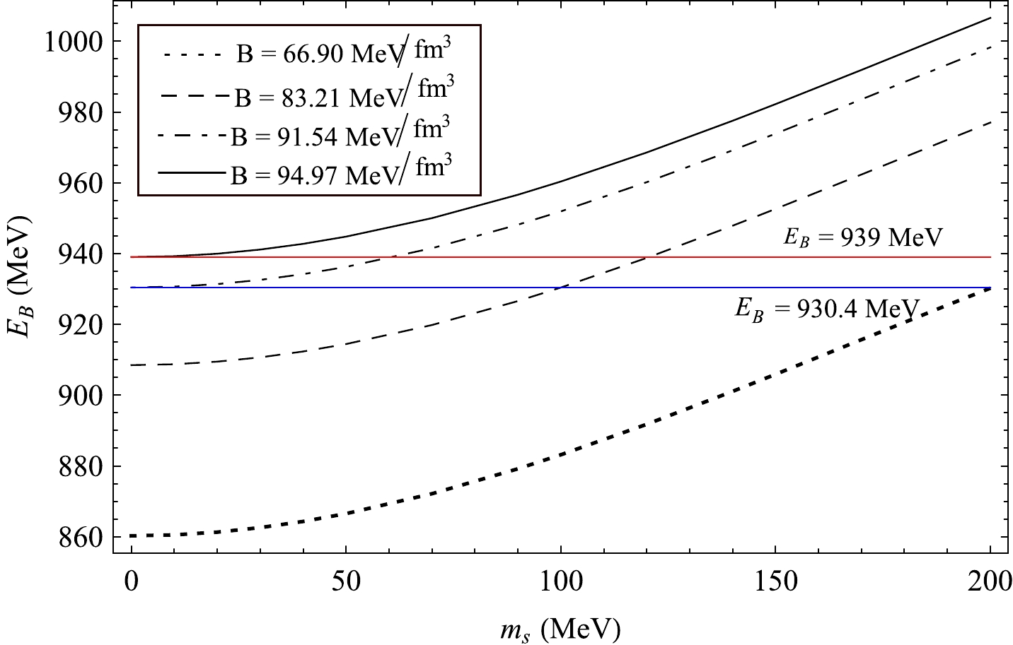
Figure 1. (color online) Variation of energy per baryon
(EB) with strange quark mass(ms) for different value of bag constant(B) .Stability B=57.55MeV/fm3 
B=66.90MeV/fm3 
B=83.21MeV/fm3 
B=91.54MeV/fm3 
B=95.11MeV/fm3 
Stable ms<334 
ms<200 
ms<100.5 
··· ··· ( EB<930.4 MeV )
Metastable ··· ··· 100.5<ms 
0<ms 
··· ( 930.4<EB<939 MeV )
<120.3 
<60.18 
Unstable ··· ··· ms>120.3 
ms>60.18 
ms>0 
( EB>939 MeV )
Table 1. Values of B and corresponding Constraints on
ms essential for different stability windows of 3-flavor SQM. -
Let us consider the interior of the cold compact stars described by the static spherically symmetric space time metric:
ds2=−eν(r)dt2+eλ(r)dr2+r2(dθ2+sin2θdϕ2),
(12) where
eν(r) andeλ(r) are metric functions of r. In relativistic compact stars, the energy momentum tensor of the interior matter content with anisotropic fluid pressures is given byTij=diag(−ρ,pr,pt,pt),
(13) where ρ,
pr , andpt are the energy density(ρ) , radial pressure(pr) , and tangential pressure(pt) , respectively. The measure of the pressure anisotropy in this model is defined bypt−pr = Δ. Aspr andpt depend on r, Δ is also a function of r.The Einstein Field Equation (
henceforth EFE ) is given byRij−12gijR=8πGc2Tij,
(14) where
Rij = Ricci tensor andR = Ricci scalar. The left hand side represents the geometry corresponding to the energy momentum tensor of matter given in the right hand side.Using Eqs. (12) and (13) in Eq. (14), the EFEs can be represented as
e−λ(λ′r−1r2)+1r2=ρ,
(15) e−λ(1r2+ν′r)−1r2=pr,
(16) 12e−λ[12(ν′)2+ν′′−12λ′ν′+1r(ν′−λ′)]=pt,
(17) where
(′) indicates the derivative with respect to r. We have used the conventional values8πG = 1 , andc=1 . Now we consider metric anstaz as proposed in Refs. [49, 50, 55] for thegrr component characterized by two parameters denoted by a and b as given below:eλ(r)=1+ar21+br2.
(18) In Eq. (18), dimensions of constants a and b are
Km−2 . These two constants define the curvature of space time.Using Eqs. (10) and (18) in Eqs. (15)–(17), we obtain the following expression for physical parameters relevant to viable stellar configurations:
ρ=1r2+(1+br2)(−1r2+2(a−b)(1+ar2)(1+br2))1+ar2],
(19) pr=13[−4B′+1r2+(1+br2)(−1r2+2(a−b)(1+ar2)(1+br2))1+ar2],
(20) pt=(1+br2)2(1+ar2)[23XY+29X2−23[2aB′b+12(4a2r2(1+ar2)2−2a(1+ar2))+12b2(−2ab+3b2−2aB′+2bB′)×(−4b2r2(1+br2)2+2b(1+br2))+−2Y−23Xr],
(21) ν(r)=−23[aB′r2b−12log(1+ar2)+(−2ab+3b2−2aB′+2bB′)2b2log(1+br2)],
(22) and
Δ(r)=pt−pr=r29(1+ar2)3(1+br)[2(9b2+9bB′+2(B′)2)+4a4r4(−1+B′r2)2+a2(3−48br2−44B′r2+7b2r4+a3r2{15−34B′r2+16(B′)2r4+br2(−11+8B′r2)}+a{33b2r2+2B′(−9+8B′r2)+b(−21+44B′r2)}],
(23) where
X=2aB′rb−ar(1+ar2)+(−2ab+3b2−2aB′+2bB′)rb(1+br2) andY=(a−b)r(1+ar2)(1+br2) . Now we can determine the mass functionm(r) of the star from the following expression:m(r)=4π∫r0ρ(r)r2dr.
(24) Using Eq. (19), the expression of mass function in this model can be represented as
m(r)=(a−b)r32(1+ar2),
(25) Eq. (24) shows that for
m(r)>0 , we should havea>b . The following bounds on metric constants "a" and "b" should be followed in order to get a physically viable stellar model. The expression for central density(ρ0) can be found from Eq. (19) by puttingr=0 and is given below:ρ0=3(a−b).
(26) Again, from Eq. (20), we note the value of central pressure
(p0) as follows:p0(r=0)=(a−b−4B′3).
(27) -
For physically realistic models the following conditions must be satisfied:
(i) The interior metric as given in Eq. (12) should be continuous at the surface of the star, and hence, it must be equal to the exterior metric given by Schwarzschild:
ds2=−(1−2Mr)dt2+(1−2Mr)−1dr2+r2(dθ2+sin2θdϕ2).
(28) Matching the potentials at the boundary,
r=R giveseν(R)=(1−2MR),
(29) and
eλ(R)=(1−2MR)−1.
(30) From Eq. (30), one can establish the connection between the constants "a" and "b" through the relation
b=a(1−2u)−2uR2,
(31) Using Eqs. (26) and (31), we can express central density
(ρ0) as a function of the compactness(u) as given below:ρ0=6u(a+1R2),
(32) where u =
MR is defined as the compactness of the star.(ii) The radial pressure
(pr) must vanish at(r=R) . Then, using Eq. (20), the radius(R) of the star can be determined asR=√−8a+1B′−baB′−√a−b√a−b+32B′aB′2√2.
(33) From Eq. (33), it is evident that radius R depends on
ms through constantB′ as well as constants a and b.(iii) Inside a star, physical parameters like ρ,
pr andpt all have positive values.For positive central pressure
(p0>0) , we note from Eq. (27) that a lower bound on the constant "a" exists, which isa>(2B′3u−1R2).
(34) In Eq. (34), the dimension of
B′ should beKm−2 as the dimensions of a and R areKm−2 andKm , respectively, and u is dimensionless. As B is given inMeV/fm3 , we have to divide B by the factor(3×10⁴) to get the dimensionKm−2 . AccordinglyB′ can be expressed inKm−2 .(iv) The gradient of energy-density and the pressure must be negative inside the star, i.e.,
(dρdr)<0 ,(dprdr)<0 and(dptdr)<0 .(v) Both the pressures (radial and tangential) are same at the centre
(r=0) , and therefore,Δ=0 at the centre of the star.(vi) The square of radial
(v2r=dprdρ) and tangential(v2t=dptdρ) sound velocities should lie within the range0≤v2r≤1 and0≤v2t≤1 . -
Buchdahl predicted that the maximum value of mass to radius ratio (compactness) should obey the relation
M/R≤49 [56]. From Eq. (19), it is noted that the central density of a star is related to the constants of the metric parameters through the relationρ0=3(a−b) . Therefore, for a given central density(ρ0) , the mass function given in Eq. (25) can be written asm(r)=ρ0r36(1+ar2).
(35) For a stellar configuration to be stable, the mass
(M) of a star should increase with central density(ρ0) , i.e.,(∂M/∂ρ0)>0 [57, 58]. In presence of small perturbation, the condition(∂M/∂ρ0)<0 corresponds to an unstable stellar model. In Figs. 2 and 3, we have shown the mass-radius plot for two chosen values of the bag constant(B) , e.g.,B=57.55 and91.54 MeV/fm3 , respectively. In both cases, the maximum mass is found to reach its maximum value whenms→0 MeV . It is noted that the maximum mass may be as high as2.01M⊙ whenB=57.55 MeV/fm3 and1.60 M⊙ whenB=91.54 MeV/fm3 . The corresponding radii are10.96 km and8.69 km , respectively. Again, keeping B fixed, we note that higher values ofms admit lower maximum mass as evident from Figs. 2 and 3. We note that whenB=57.11 MeV/fm3 andms=150 MeV , the maximum mass = 1.93M⊙ , and whenB=91.54MeV/fm3 andms= 150 MeV, the maximum mass = 1.54M⊙ . Dependence of maximum mass on the value ofms can be explained from the concept of equation of state. The corresponding central densities(ρ0) assume the values1.98×1015 gm/cm3 and3.13×1015 gm/cm3 , respectively, as evident from Figs. 4 and 5 whereB=57.55 and91.54 MeV/fm3 , respectively. We note that though the maximum mass is less whenB=91.54 MeV/fm3 , its compactness is slightly greater, and as a result, its central density becomes greater than whenB=57.11 MeV/fm3 . This is also verified from Eq. (32). Figures 4 and 5 also indicate that after reaching the point of maximum mass, star mass decreases with an increase in central density. Therefore, the stability criterion(∂M/∂ρ0)>0 is valid only up to the maximum mass point. It is evident from Fig. 6 that a higher value ofms admits a softer EoS of matter, and consequently, the maximum mass becomes smaller for higher values ofms .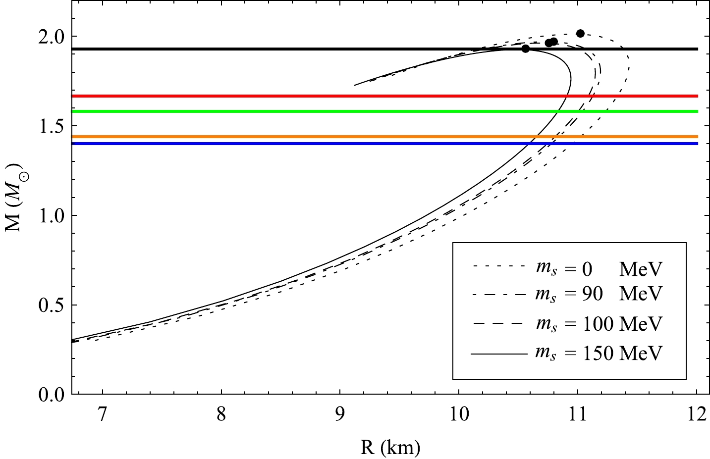
Figure 2. (color online) Mass vs. radius curve for strange quark star for different strange quark mass
(ms) for a fixed bag constantB=57.55 MeV/fm3 . The maximum mass points are filled by black points. Here, the black, red, green, orange, and blue lines represent the observed masses of PSR J1614-2230, PSR J1903+0327, 4U 1820-30, PSR J0030+0451, and GW170817, respectively.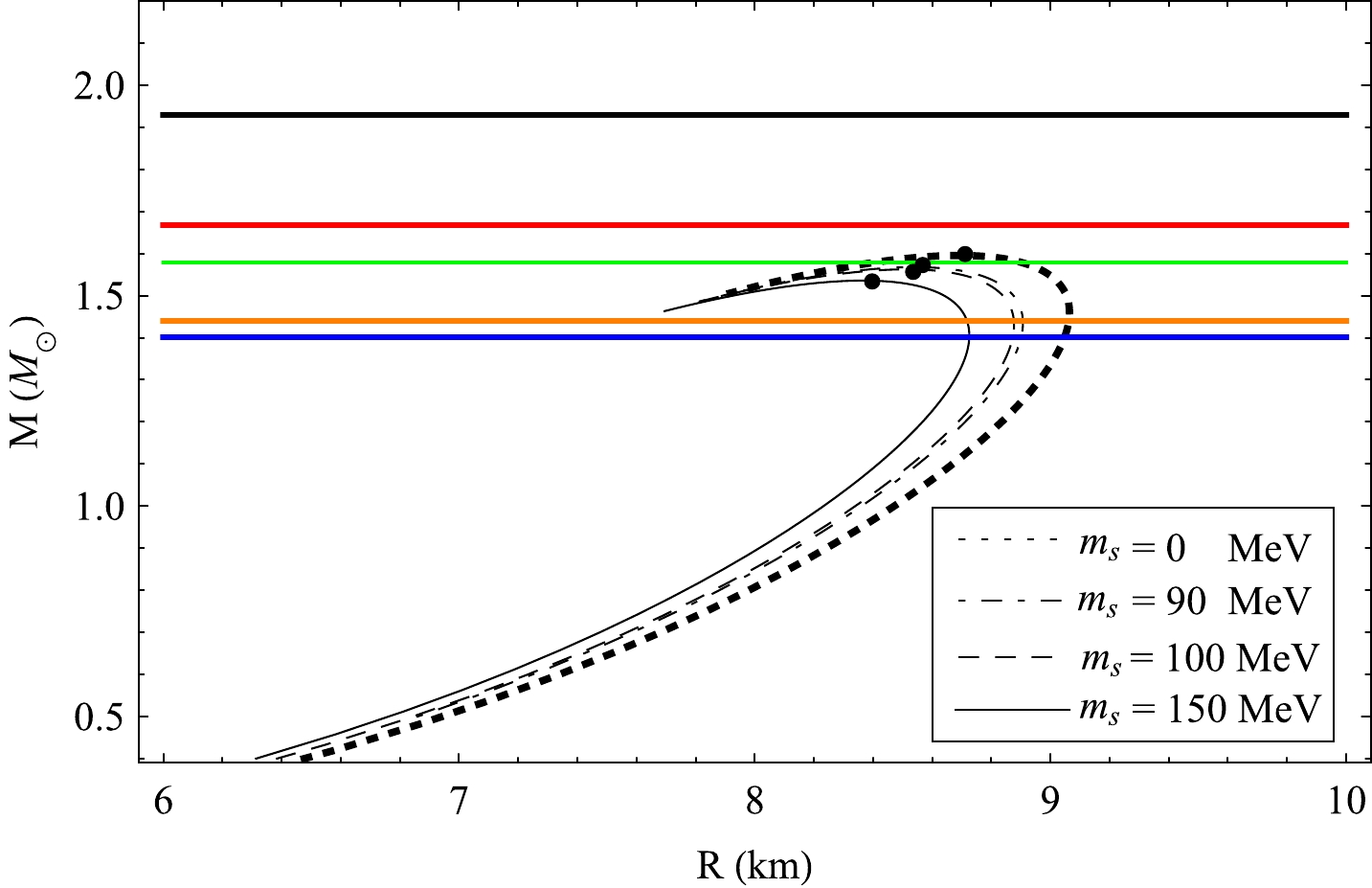
Figure 4. Mass vs. central density curve for strange quark star for different strange quark mass
(ms) for a fixed bag constantB=57.55 MeV/fm3 . The maximum mass points are filled by black points.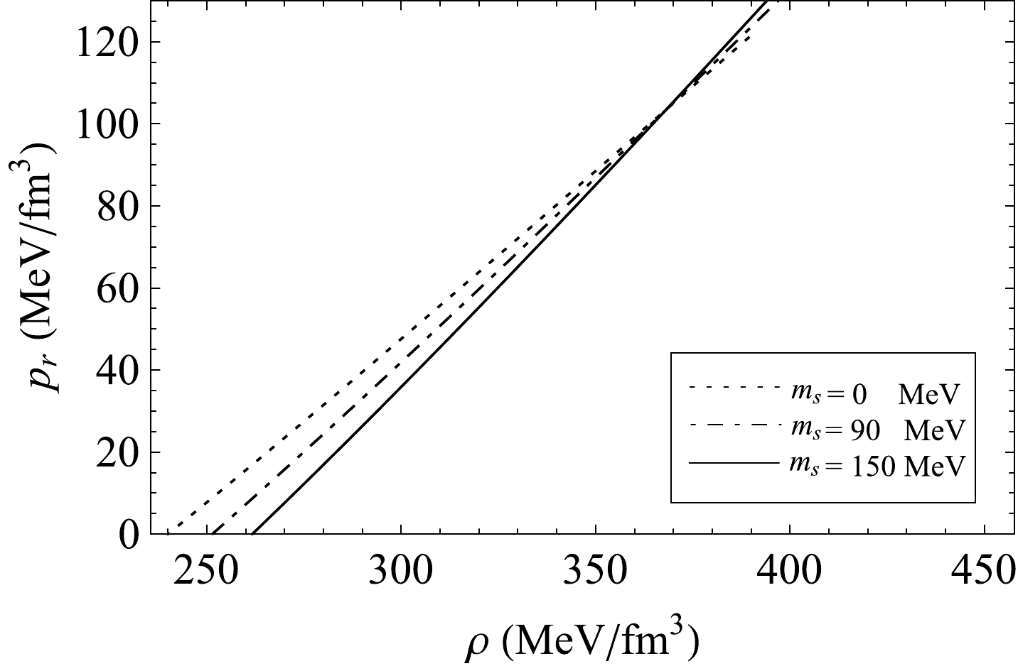
Figure 6. Variation of radial pressure
(pr) with energy density(ρ) for different values of strange quark mass(ms) for an arbitrary bag constantB=60 MeV/fm3 .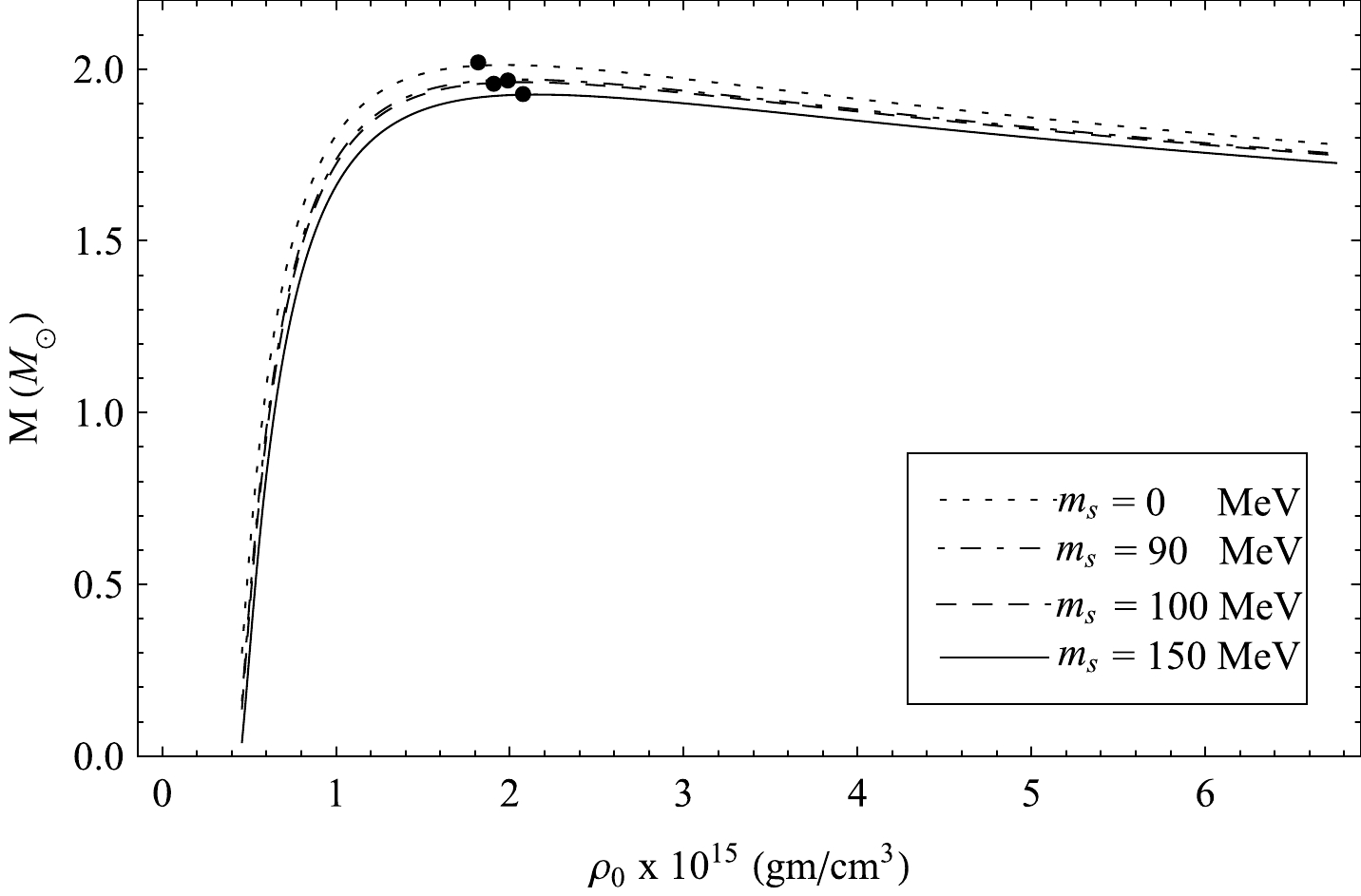
Figure 3. (color online) Mass vs. radius curve for strange quark star for different strange quark mass
(ms) for a fixed bag constantB=91.54 MeV/fm3 . The maximum mass points are filled by black points. Here the black, red, green, orange, and blue lines represent the observed masses of PSR J1614-2230, PSR J1903+0327, 4U 1820-30, PSR J0030+0451, and GW170817, respectively.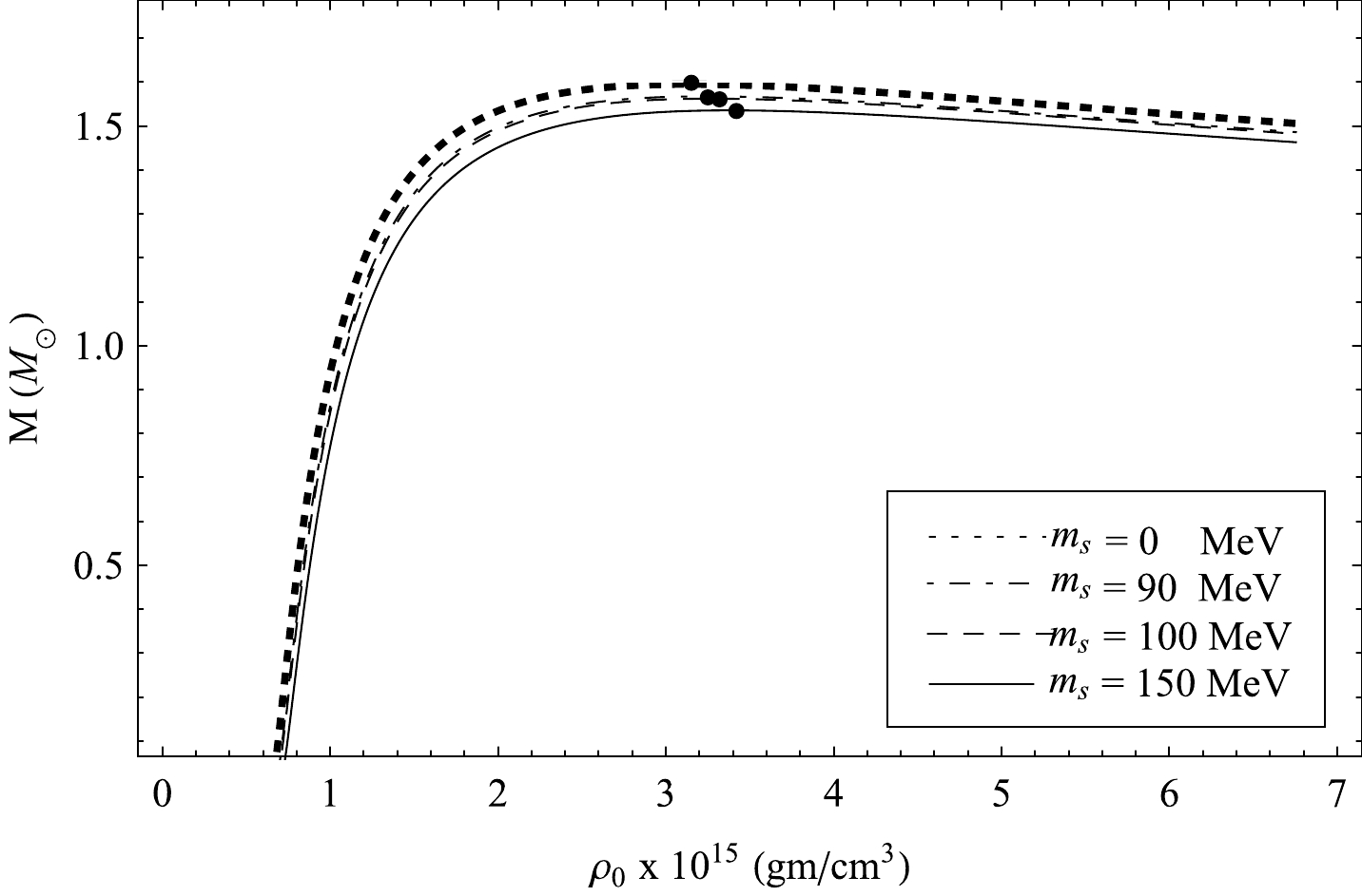
Figure 5. Mass vs. central density curve for strange quark star for different strange quark mass
(ms) for a fixed bag constantB=91.54 MeV/fm3 . The maximum mass points are filled by black points. -
Case I: Now, we consider the compact object PSR J1614-2230, which is supposed to be an SQS having an observed mass 1.97
M⊙ [47]. We have predicted the radius of PSR J1614-2230 from our proposed model and tabulated the same in Table 2. We have noted that the radius(R) of the star depends on the mass(ms) of the strange quark, and the value of B. From Table 2, it is observed that the radius of PSR J1614-2230 may be predicted for different combinations of a, B, andms . It is also noted that the predicted radius decreases when B andms increase. We have also determined the binding energy per baryon(EB) for different combinations of B andms and listed the same in Tables 2 and 3. We may conclude that the stability of SQM is a function of both B andms . Energy per baryon increases with the increase in B andms . An interesting feature is that the mass ofms cannot be increased arbitrarily depending on the value of B. For example, whenB=57.55 , the value ofms should lie below 290 MeV to get stable SQM. However, when290<ms<334 MeV , SQM becomes metastable, and forms> 334 MeV, SQM is unstable. However, with increasing B, these stability windows change and occur at different values ofms , as shown in Tables 2 and 3. We have noted that beyond a certain value ofB(=91.54 MeV/fm3) , SQM becomes unstable for any value ofms [59]. The variations of different physical parameters, namely energy density(ρ) , radial pressure(pr) , tangential pressure(pt) , and pressure anisotropy(Δ) are also shown in Figs. 7− 10 for different values ofms . We note that all the physical parameters are well behaved for the chosen value of different parameters. In Figs. 11 and 12 we have shown the variation of density and pressure gradients inside PSR J1614-2230.B/(MeV/fm3) 
a ms/MeV 
EB/MeV 
Predicted radius (R) 
Stability 57.55 0.01 0 828.49 11.25 stable 50 834.98 11.21 stable 100 852.07 11.10 stable 290 930.37 11.07 stable 334 933.89 11.05 metastable 70 0.015 0 870.06 10.33 stable 50 876.26 10.29 stable 150 915.39 10.09 stable 180 930.07 10.04 stable 190 934.94 10.03 metastable 199 939.25 10.02 unstable 205 942.09 10.02 unstable 90 0.023 0 926.48 9.31 stable 40 930.26 9.29 stable 50 932.33 9.28 metastable 75 939.45 9.25 unstable 100 948.06 9.20 unstable 150 970.07 9.11 unstable 91.54 0.023 0 930.42 9.27 metastable 50 936.24 9.24 metastable 100 951.92 9.16 unstable 150 973.89 9.07 unstable Table 2. Predicted radius for the compact object PSR J1614-2230 with mass 1.97
M⊙ .B/(MeV/fm3) 
a ms/MeV 
EB/MeV 
Predicted radius (R) stability 57.55 0.008 0 828.49 11.10 stable 50 834.98 11.05 stable 100 852.07 10.94 stable 150 875.14 10.82 stable 290 930.37 10.91 stable 80 0.015 0 899.60 9.65 stable 50 905.61 9.61 stable 100 921.69 9.53 stable 120 930.11 9.50 stable 121 930.54 9.49 metastable 140 939.25 9.45 unstable 150 944.01 9.43 unstable 90 0.015 0 926.48 9.33 stable 40 930.26 9.31 stable 50 932.33 9.30 metastable 75 939.17 9.26 unstable 100 948.10 9.22 unstable 150 970.10 9.13 unstable 91.54 0.015 0 930.42 9.29 metastable 50 936.24 9.25 metastable 100 951.92 9.18 unstable 150 973.89 9.09 unstable Table 3. Predicted radius for the compact object Vela X-1 with mass 1.77
M⊙ .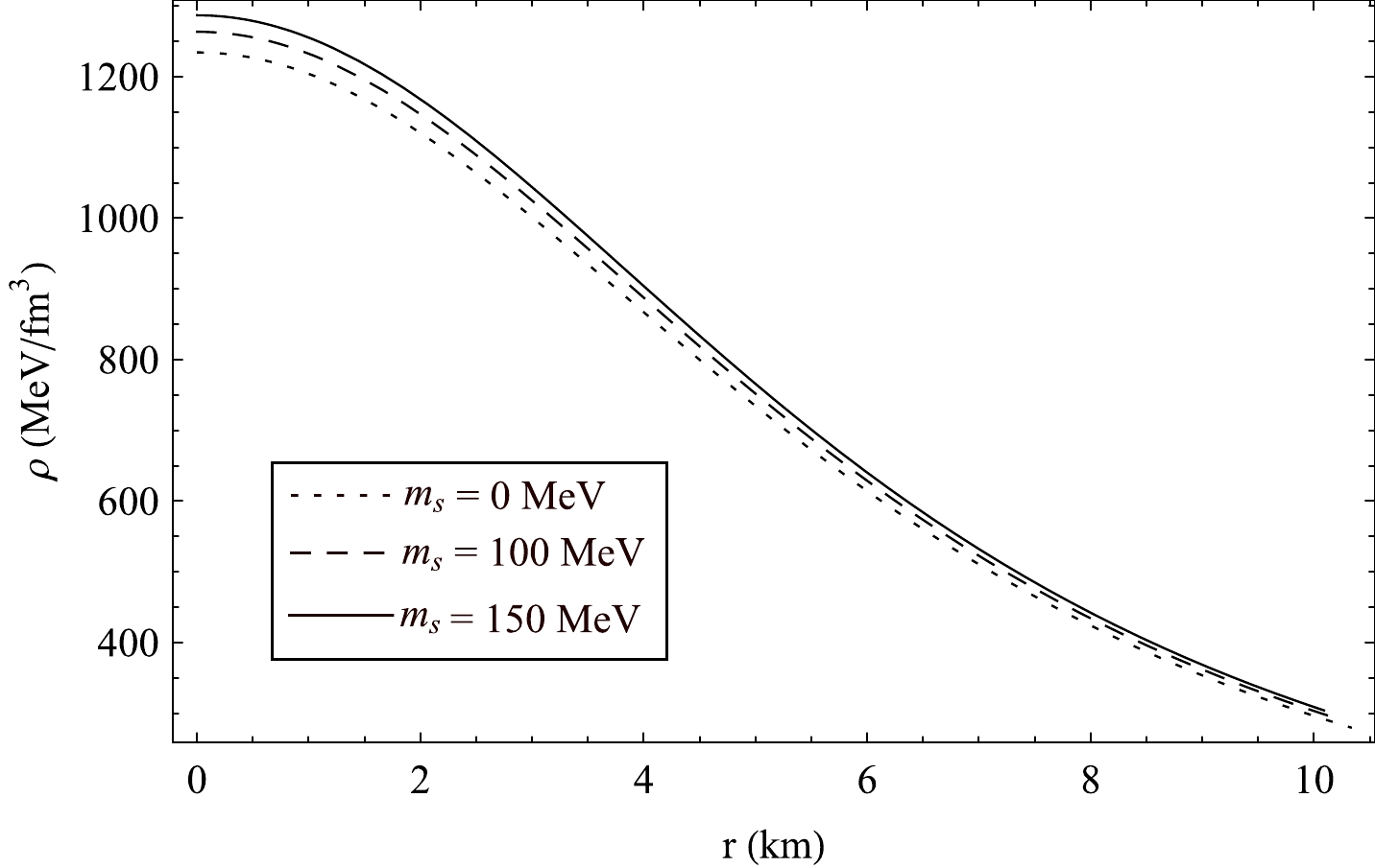
Figure 7. Variation of ρ with r in PSR J1614-2230 for different values of strange quark mass
(ms) and B = 70MeV/fm3 .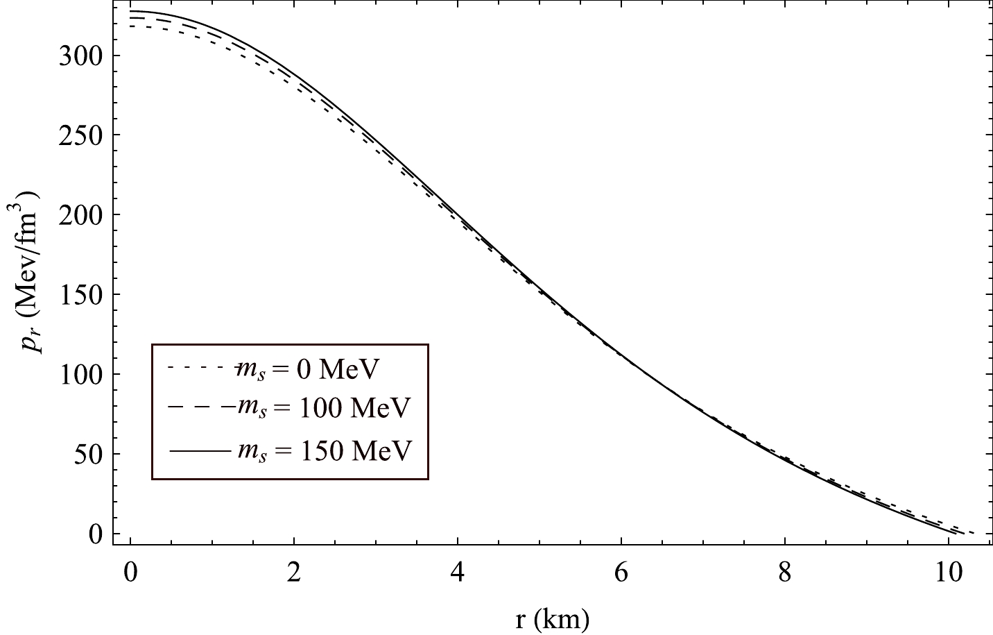
Figure 8. Variation of
pr with r in PSR J1614-2230 for different values of strange quark massms and B = 70MeV/fm3 .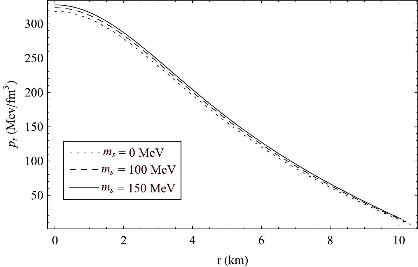
Figure 9. (color online) Radial variation of tangential pressure
pt in PSR J1614-2230 for different values of strange quark massms and B = 70MeV/fm3 .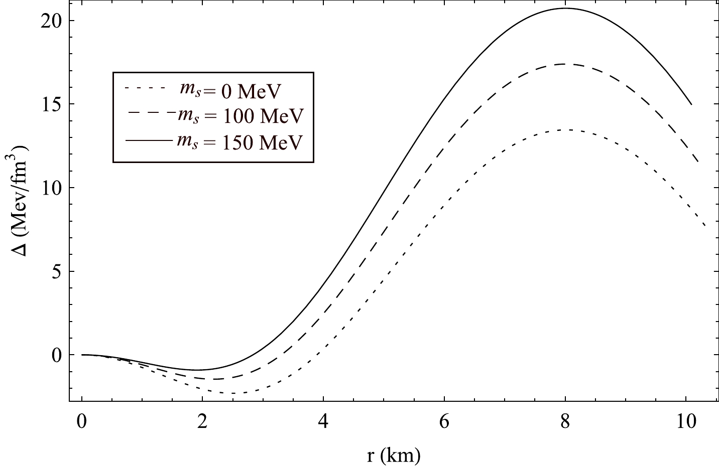
Figure 10. Radial variation of Δ in PSR J1614-2230 for different values of strange quark mass
ms and B = 70MeV/fm3 .
Figure 11. Behavior of energy density gradient (
dρ/dr ) in PSR J1614-2230 with B =70 MeV/fm3 for differentms .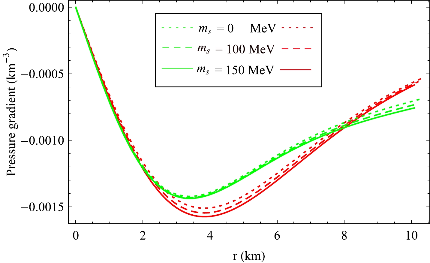
Figure 12. (color online) Behavior of different pressure gradients in PSR J1614-2230 with B =
70 MeV/fm3 for differentms . Here red and green colours represent (dpr/dr ) and (dpt/dr ) respectively.Case II: Consider another low mass X-ray binary star Vela X-1 of observed mass 1.77
M⊙ [60]. We have calculated its radius from our proposed model and tabulated the same in Table 3. The radial variation of different physical parameters like energy density(ρ) , radial pressure(pr) , tangential pressure(pt) and pressure anisotropy(Δ) are also plotted in Figs. 13−16 respectively. In Figs. 17 and 18 we have shown the variation of density and pressure gradients inside Vela X-1.
Figure 13. Radial variation of energy density
(ρ) in Vela X-1 for different values of strange quark mass(ms) and B = 80MeV/fm3 .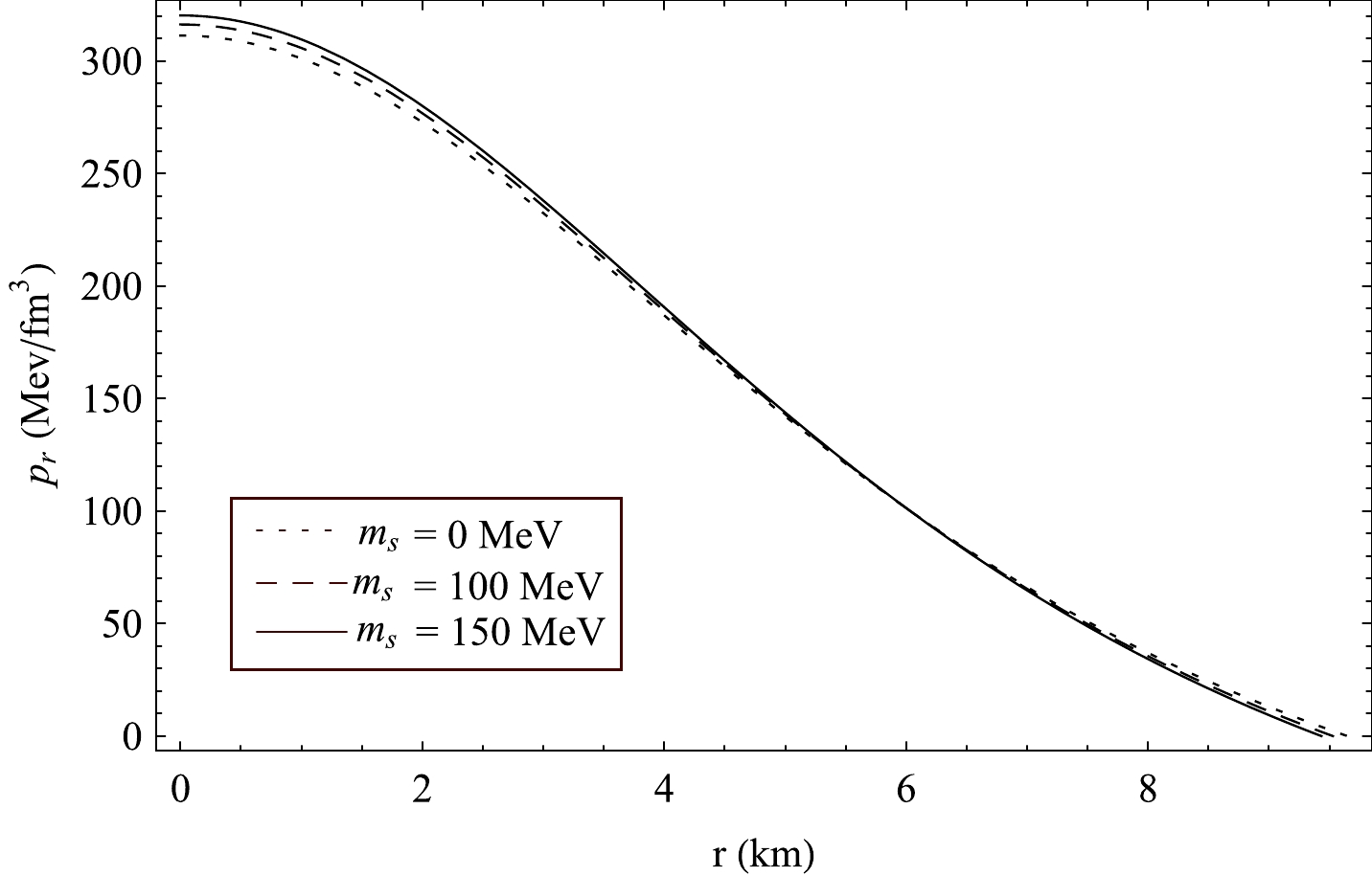
Figure 14. Radial variation of radial pressure
pr in Vela X-1 for different values of strange quark massms and B = 80MeV/fm3 .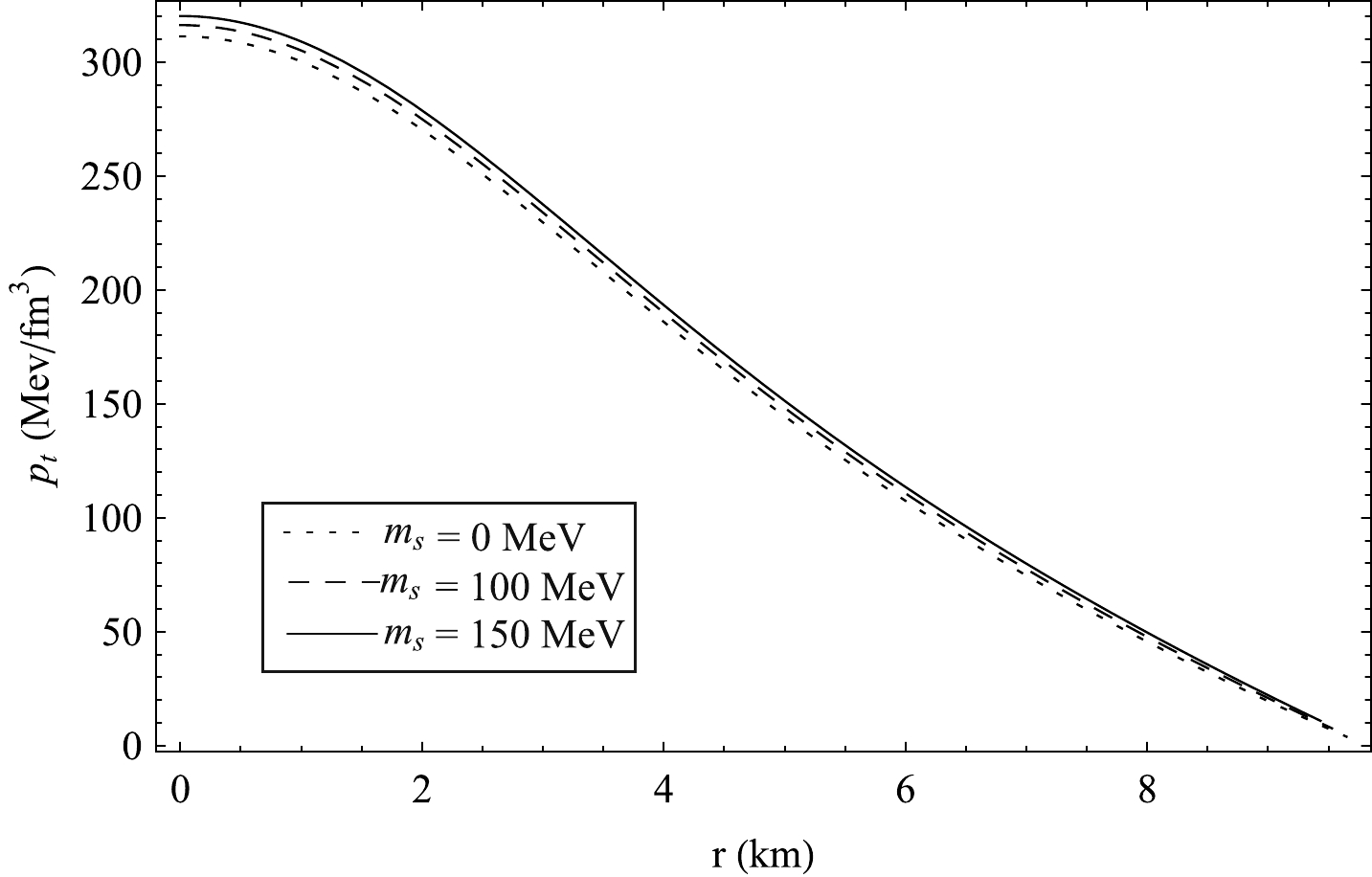
Figure 15. (color online) Radial variation of tangential pressure
pt in Vela X-1 for different values of strange quark massms and B = 80MeV/fm3 .
Figure 16. Radial variation of Δ in Vela X-1 for different values of strange quark mass
ms and B = 80MeV/fm3 .
Figure 17. Behavior of energy density gradient (
dρ/dr ) in Vela X-1 with B =80 MeV/fm3 for differentms .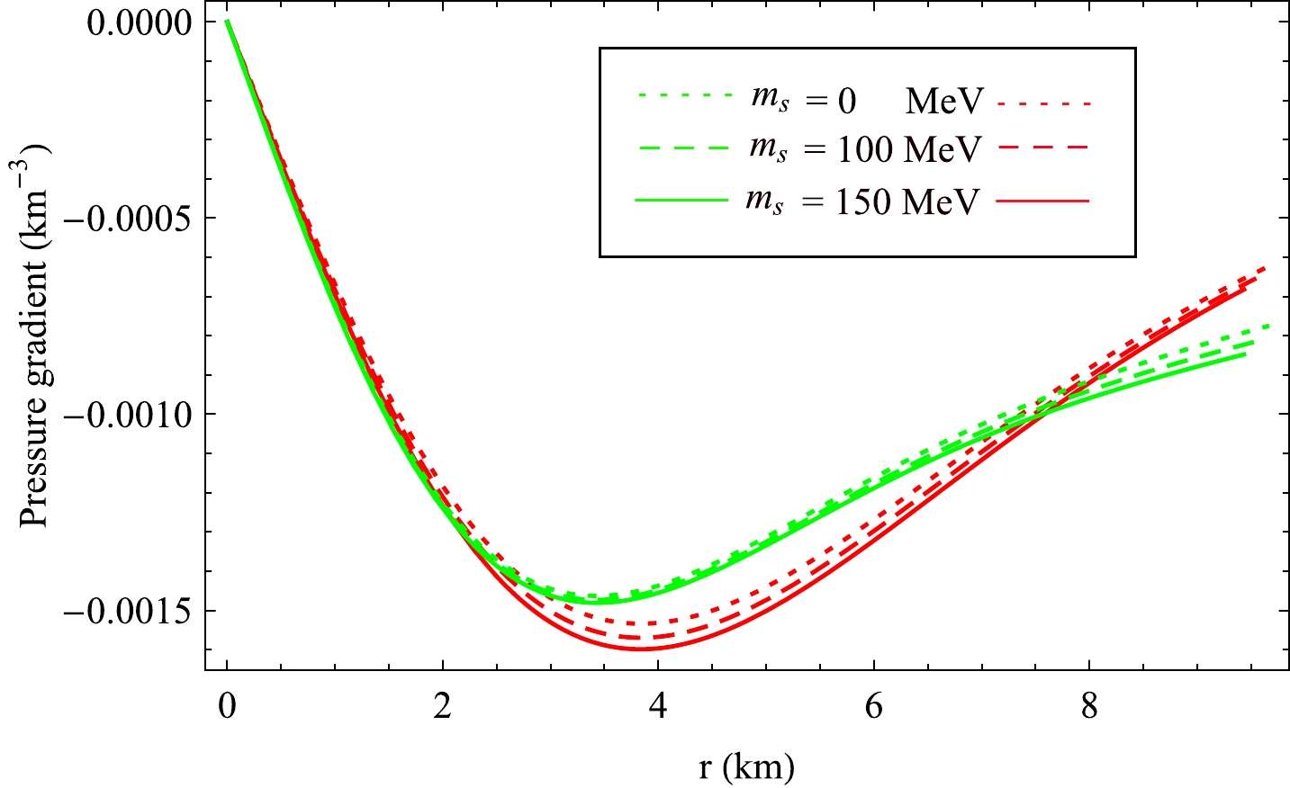
Figure 18. (color online) Behavior of different pressure gradients in Vela X-1 with B =
80 MeV/fm3 for different values ofms . Here, red and green colours represent (dpr/dr ) and (dpt/dr ) , respectively. -
For any fluid sphere that is anisotropic in nature, all the energy conditions [61, 62], such as the
(i) weak energy condition (WEC),(ii) null energy condition (NEC),(iii) strong energy condition (SEC), and(iv) dominant energy condition (DEC), must be fulfilled throughout the interior of the fluid sphere. These are expressed mathematically as shown below.1. NEC:
ρ+pr≥0 andρ+pt≥0 .2. WEC:
ρ≥0 ,ρ+pr≥0 , andρ+pt≥0 .3. SEC:
ρ+pr≥0 ,ρ+pt≥0 and(ρ+pr+2pt)≥0 .4. DEC:
ρ≥0 ,(ρ−pr)≥0 and(ρ−pt)≥0 .From Figs. 19−23, it is found that all the necessary energy conditions are valid in this approach.
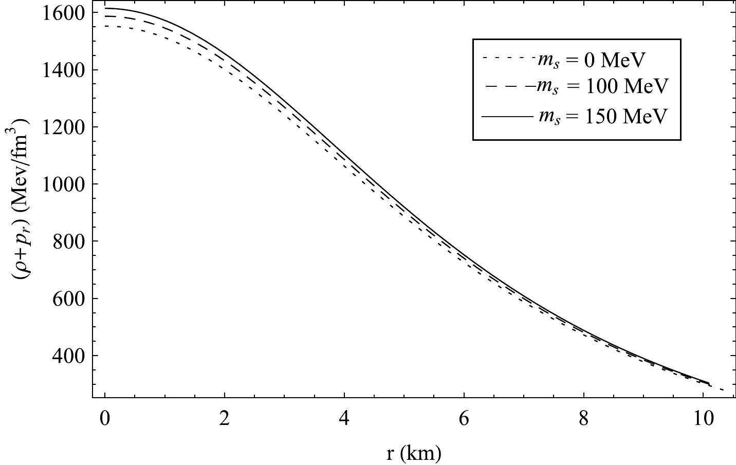
Figure 19. Radial variation of
(ρ+pr) in PSR J1614-2230 for different values of strange quark mass(ms) and B = 70MeV/fm3 .
Figure 20. Radial variation of
(ρ−pr) in PSR J1614-2230 for different values of strange quark massms and B = 70MeV/fm3 .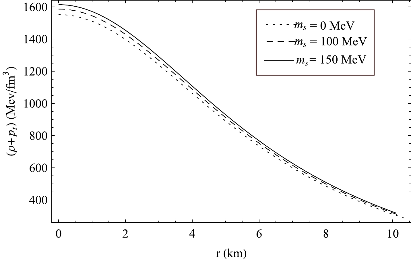
Figure 21. Radial variation of
(ρ+pt) in PSR J1614-2230 for different values of strange quark massms and B = 70MeV/fm3 .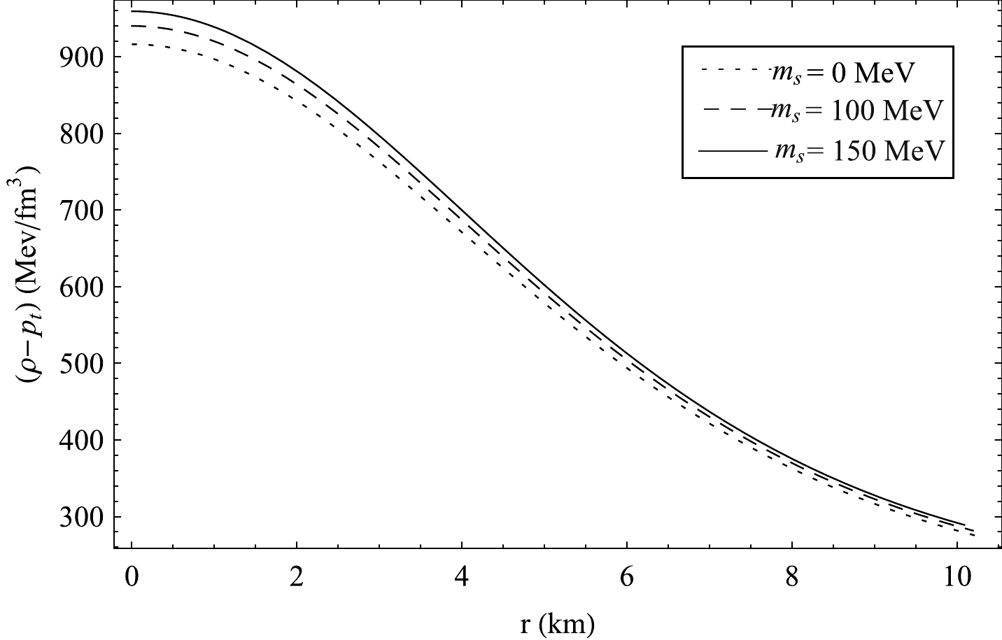
Figure 22. Radial variation of
(ρ−pt) in PSR J1614-2230 for different values of strange quark massms and B = 70MeV/fm3 .
Figure 23. Radial variation of
(ρ+pr+2pt) in PSR J1614-2230 for different values of strange quark massms and B = 70MeV/fm3 . -
For any stellar model to be viable it, must satisfy the stability criterion of the configuration within the parameter space used to define the model. We have discussed stability in light of the following analyses:
1. Verification of Tolman-Oppenheimer and Volkoff equation.
2. Fulfillment of cracking condition proposed by Herrera.
3. Value of adiabatic index
(Γ)>4/3 (Newtonian limit). -
According to Tolman [63] as well as Oppenheimer and Volkoff [5], the sum of the three forces, namely the gravitational
(Fg) , hydrostatic(Fh) , and anisotropic(Fa) , should be equal to zero, in stable equilibrium, throughout the interior of the compact object, i.e.,Fg+Fh+Fa=0.
(36) The generalized form of the TOV equation [64, 65] is
−Mg(ρ+pr)r2eλ−ν2−dprdr+2r(pt−pr)=0,
(37) where
Mg denotes the effective gravitational mass within the radius r of a stellar configuration expressed asMg=12r2eν−λ2ν′,
(38) where
ν′=dν/dr , and at any point r inside a stellar structure, gravitational forceFg comes from the effective mass(Mg) of the spherical region of radius r following the relation given in Eq. (38). For the present model,Fg=−12(ρ+pr)ν′,
(39) Fh=−dpr(r)dr,
(40) Fa=2(pt−pr)r.
(41) In this paper, the units used for ρ,
pr andpt areMeV/fm3 . Now, as the metric potential ν is unitless, its derivativeν′=dν/dr has the unitKm−1 . Again ρ,pr , andpt can be expressed in the unitsKm−2 using the transformation1 Km−2=3×10⁴ MeV/fm3 [66]. Therefore, in view of Eqs. (39)−(41), the forces (Fg ,Fh , andFa ) can be expressed in the unit ofKm−3 . In Fig. 24, we have presented the variation ofFg ,Fh , andFa with radial distance obtained from Eqs. (39)−(41), respectively, withms= 0, 100, 150 MeV for PSR J1614-2230. From these plots, it is ovious that inside the stellar configuration, static equilibrium is established under the combined effect of the above three forces. We note that combined effects of hydrostatic(Fh) and anisotropic(Fa) forces jointly balance the gravitational forceFg , to make the resultant of these forces equal to zero in the interior, as well as on the surface, of the compact objects. We have also noted that the anisotropic force(Fa) increases from centre to surface monotonically. In contrast, both the gravitational(Fg) and hydrostatic(Fh) forces increase from the centre, assume a maximum value between the centre and surface, and then decrease up to the surface. A similar type of variation is also reported by Maurya et al. [67] for different compact objects in four dimensional space-time geometry.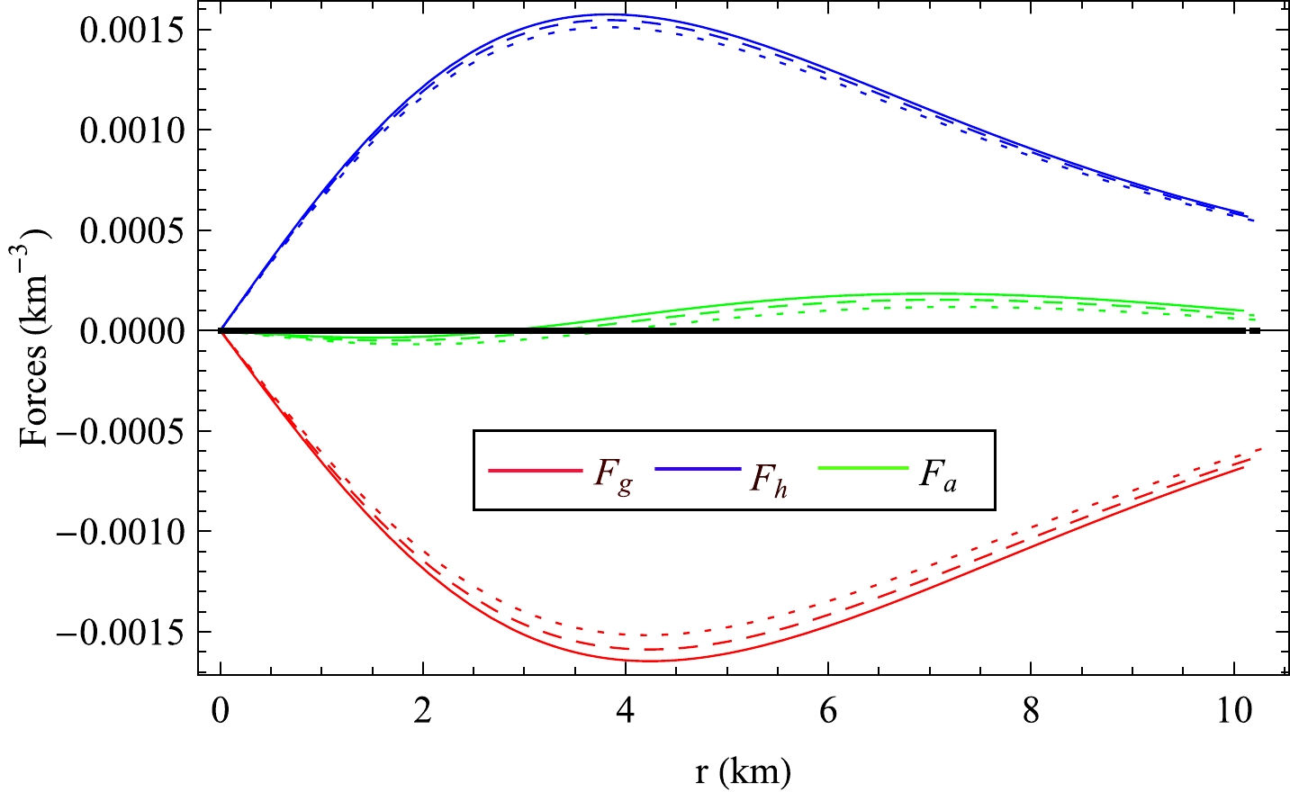
Figure 24. (color online) Radial variation of different forces of PSR J1614-2230 for
B=70 MeV/fm3 . Here, the dotted line representsms=0 , dashed line representsms=100 , and solid line representsms=150 . -
To satisfy the causality conditions, the squares of the radial
(v2r) and the tangential sound velocities(v2t) should lie within the ranges0≤v2r≤1 and0≤v2t≤1 , respectively. Fulfillment of causality conditions is evident fromFig. 25 inside PSR J1614-2230. To check the stability criterion of anisotropic matter distribution inside a compact object, Herrera [68] first suggested the "Cracking condition" concept. Based on Herrera's concept, Abreu et al. [69] gave a criterion that states that, for any stellar model, the following inequility should be satisfied: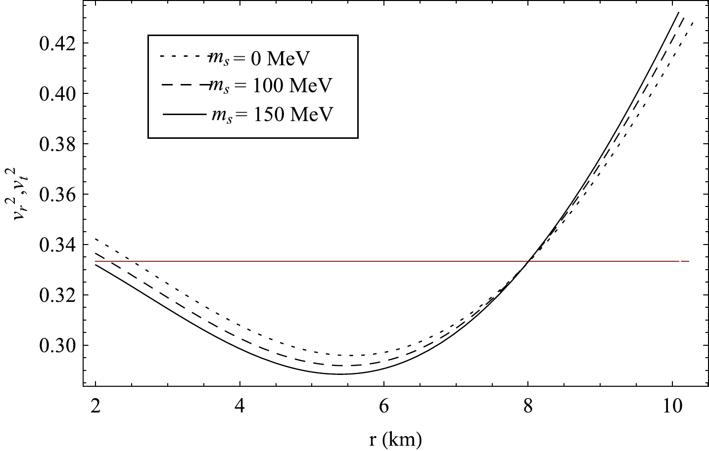
Figure 25. (color online) Radial variation of square of the radial
(v2r) and tangential(v2t) sound velocities in PSR J1614-2230 forB=70 MeV/fm3 . Plot in red representsv2r and black representsv2t for different values ofms .0≤|v2t−v2r|≤1.
(42) Eq. (42) is also known as the Abreu inequality. We have plotted the value of
|v2t−v2r| with r for PSR J1614-2230 and shown in Fig. 26 that the Abreu inequality is satisfied at all points inside the star PSR J1614-2230.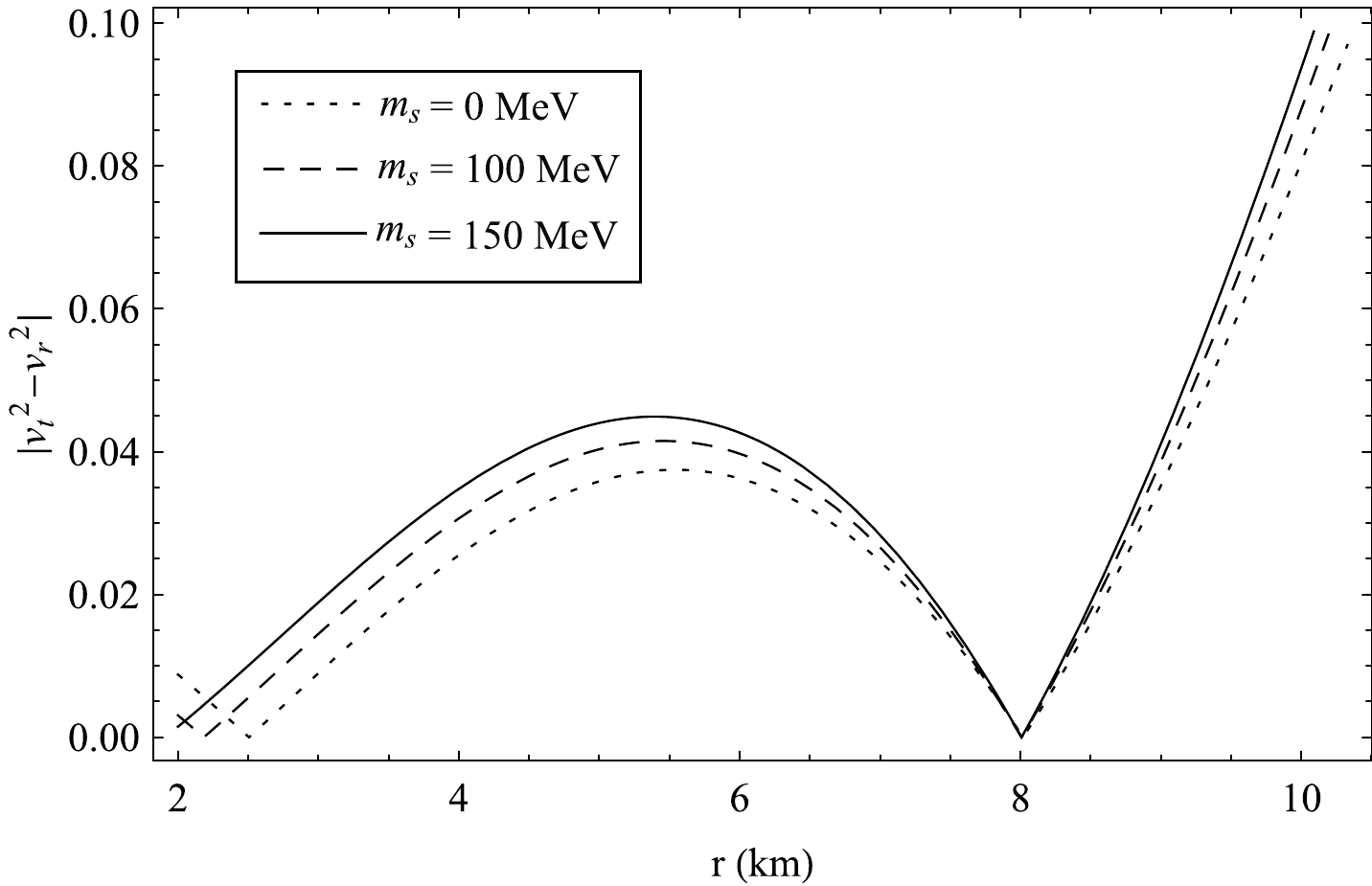
Figure 26. Radial variation of
|v2t−v2r| in PSR J1614-2230 for different values ofms forB=70 MeV/fm3 . -
An isotropic star adiabatic index
(Γ) is defined by the following relation:Γ=ρ+prpr(dprdρ)=ρ+prprv2r,
(43) where
pr is the radial pressure.According to Heintzmann and Hillebrandt [70], for any isotropic stellar structure to be stable, the adiabatic index must be within the Newtonian limit, i.e.,
Γ>4/3 . Chan et al. [71] modified this condition for an anisotropic star, where radial pressure(pr) and tangential pressure(pt) exist. For such a star,Γ>Γ′max , whereΓ′max=43−[43(pr−pt)|p′r|r]max.
(44) The necessary and sufficient condition for anisotropic stellar structure stability is that the adiabatic index
(Γ) be greater thenΓ′max . The adiabatic index Γ for PSR J1614-2230 in Fig. 27 shows that the value of the adiabatic index satisfies the stability criterion.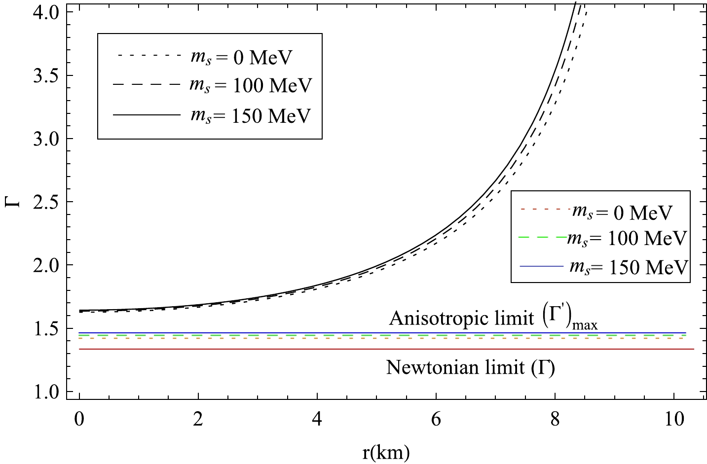
Figure 27. (color online) Radial variation of adiabatic index
(Γ) in PSR J1614-2230 for different values ofms atB=70 MeV/fm3 . Here, the red line represents the valueΓ=4/3 (Newtonian limit). -
We have also studied the stability criterion of a stellar structure with respect to small radial oscillation. The absolute value of Lagrangian perturbation
|Δpr(R)| of radial pressure atr=R of the star against frequency (ω2 ) is plotted in Figs. 28 and 29 for PSR J1614-2230 and Vela X-1, respectively. We have adopted the technique proposed by Pretel [72]. The infinitesimal radial mode of oscillation can be expressed by two coupled equations: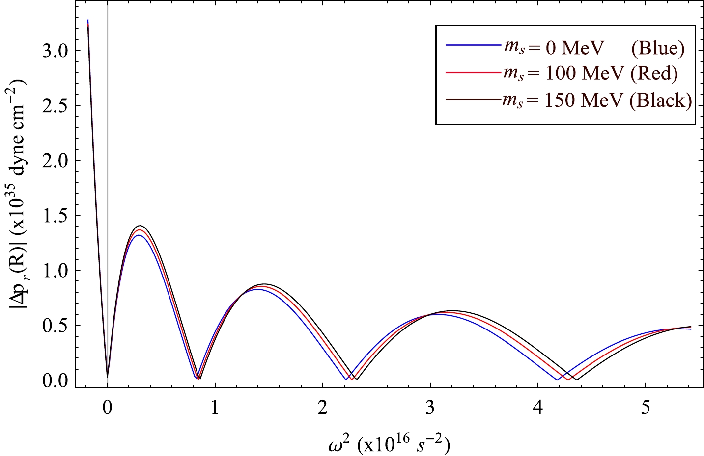
Figure 28. (color online) Variation of absolute value of the Lagrangian change in radial pressure at the surface
|Δpr(R)| vs.ω2 for different combinations ofms for the compact object PSR J1614-2230.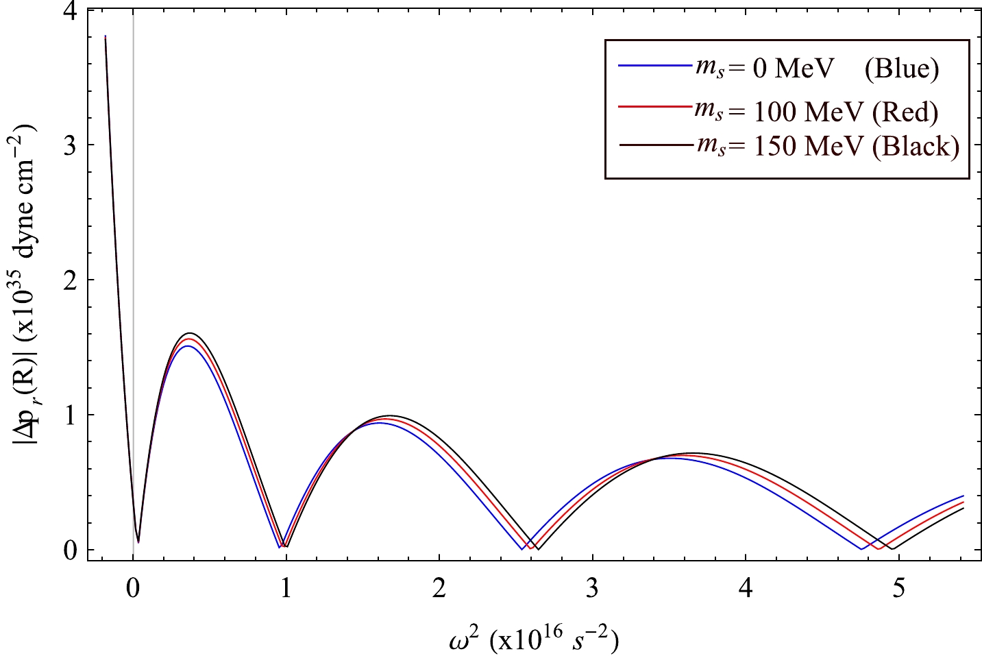
Figure 29. (color online) Variation of absolute value of the Lagrangian change in radial pressure at the surface
|Δpr(R)| vs.ω2 for different combinations ofms for the compact object Vela X-1.dχdr=−1r(3χ+ΔprΓpr)+dνdrχ,
(45) and
d(Δpr)dr=χ[ω2c2e(λ−ν)(ρ+pr)r−4dprdr−8πGc4(ρ+pr)eλrpr+r(ρ+pr)(dνdr)2]−Δpr[dνdr+4πGc4(ρ+pr)reλ].
(46) The eigenfunction represented by χ is associated with the radial segment of the Lagrangian displacement and is denoted by
χ=δ(r)r . Here, we have adopted normalized eigenfunctions χ such thatχ(0)=1 at the centre. Owing to the term (1/r ) in Eq. (45), there is a singularity atr=0 . To avoid the singularity, the coefficient of (1/r ) in the right hand side of Eq. (45) should vanish, givingΔpr=−3Γχpr as r→0.
(47) Again, as the radial pressure goes to zero at the stellar surface (
r=R ), the corresponding Lagrangian change in radial pressure should also be zero, i.e.,Δpr=0 as r→R.
(48) In this work, the variations of Lagrangian change in radial pressure at the stellar surface of PSR J1614-2230 and Vela X-1 are plotted as a function of
ω2 . The minima of these plots represent the exact normal mode frequencies. It is observed that, for the lowest normal mode,ω20>0 ; thus, our model stays in static equilibrium against small radial perturbations too. -
The distortion of the spherical shape of the surface of a compact object due to external perturbing gravity field is measured by a parameter known as the Tidal Love Number denoted by
k2 . Tidal de-formability (Λ) is also a measure of surface distortion, which is associated with the Tidal Love Numberk2 by the relation given below:k2=32Λ(MR)5,
(49) where M is the mass of compact object, and R its radius. The expression for the even parity
(l=2) Tidal Love Number (TLN) evaluated by Hinderer et al. [73] is given below:k2=8u55(1−2u)2[2+2u(g−1)−g]×[2u[6−3g+3u(5g−8)]+4u3[13−11g+u(3g−2)+2u2(1+g)]+3(1−2u)2[2−g+2u(g−1)]log(1−2u)]−1,
(50) here, u is known as compactness
(=MR) andg=bH′(R)H(R) .H(R) is the value ofH(r) atr=R (surface). The dash represents the derivative with respect to r. The expression ofH(r) [74] is given belowH(r)=c1(rM)2(1−2Mr)[−M(M−r)(2M2+6Mr−3r2)r2(2M−r)2+32log(rr−2m)]+3c2(rM)2(1−2Mr).
(51) The binary neutron star merger event GW170817 has placed some constraints on Λ and has been predicted by Abbott and Abbott [75]. For a star of
1.4M⊙ , the Tidal de-formability should beΛ<800 as shown in the article [76]. In Table 5, the Tidal Love Number and Tidal de-formability of the companion star in the GW170817 event of mass1.4M⊙ forms=90 and 100 MeV are listed. It is noted that the Tidal de-formability (Λ) lies with in the range70<Λ1.4<580 .Star Observed mass ( M⊙ )
ms/MeV 
B /(MeV/fm3) 
Predicted radius (R)/Km 
u k2 
Λ GW170817 [80] 1.4 90 57.55 11.53 0.1790 0.1013 367.065 91.54 9.91 0.2083 0.0838 142.417 100 57.55 11.50 0.1796 0.1022 365.118 91.54 9.89 0.2088 0.0836 140.456 Table 5. Value of Tidal de-formability in our model within the parameter space used.
-
In this article, we have analyzed a class of strange stars described by the generalised MIT bag model EoS of the type
ρ=3p+4B+ρs−3ps and included the effect of the strange quark mass(ms) . Employing the Vaidya-Tikekar [49, 50] type metric ansatz, we have solved the EFE for perfect fluids having an anisotropic pressure distribution. Thegrr component of the Vaidya-Tikekar metric is characterised by two parameters a and b, which define the curvature of spacetime attached to a compact object. The allowed values of bag constant B are restricted to the range 57.55−91.54 MeV/fm3 , in which quark matter composed of three quarks (u, d, and s) is absolutely stable with respect to neutrons [59]. In this model, the expressions for various physical parameters are found to be explicitly dependent on the bag constant B and strange quark massms . In our study, some constraints on the maximum value of B andms were noted. For example, whenB=57.55 MeV/fm3 , the maximum allowed value ofms is334 MeV . Above this value, strange quark matter will be metastable or unstable. In contrast, whenms = 0, B should lie below or at91.54 MeV/fm3 to get stable strange quark matter. We have evaluatedEB to study the stability of strange quark matter inside an SQS for different values ofms . TheEB vs.ms plot for a given B is shown in Fig. 1, and the results are compared to the binding energy of56Fe (EB=930.4 MeV ) and nucleons (EB=939 MeV ). We have explored three distinct windows in view of stability of strange quark matter depending on the value ofms and B viz.(i) stable(ii) metastable, and(iii) unstable SQM. Corresponding values ofms and B are listed in Table 1. It is evident that a lower value ofms indicates better stability of SQM inside an SQS. Therefore, for strange quark stars having a maximum mass with stable SQM, a smaller value ofms is preferred. Using the generalized EoS, we have obtained the M-R plot as shown in Figs. 2 and 4. From the M-R plots, we have observed that the maximum mass obtained from our model isms dependent and picks up maximum values of2.01 M⊙ and1.60 M⊙ whenB=57.55 and91.54 MeV/fm3 , respectively, forms=0 MeV , which corresponds to stable SQM. Again, keeping B fixed, we noted that a higher value ofms admits a lower maximum mass of the quark star, as evident from Figs. 2 and 4. It is noted that whenB=57.55 MeV/fm3 andms=150MeV , the maximum mass is1.93M⊙ , and whenB=91.54MeV/fm3 andms= 150 MeV, the maximum mass is1.54M⊙ . It is observed thatms has some effect on the maximum mass and radius of an SQS, and both the maximum mass (Mmax ) and radius (Rmax ) decrease with increasingms . Such behavior may be explained as follows: as the maximum mass of a compact object depends strictly on the EoS of interior matter, the higher the value ofms , the softer the EoS, as evident from Fig. 6, and hence, the lower the maximum mass and radius. Such types of variation have also been reported by Li et al. [82] from a different aspect. From an article of the Particle Data Group [83], we have also evaluated the values of maximum mass as 1.97M⊙ and 1.57M⊙ forB= 57.55 and 91.54MeV/fm3 , respectively, for a reasonable value ofms=90 MeV . In Tables 2 and 3, we have presented the energy per baryon of SQM for PSR J1614-2230 and Vela X-1, respectively. It is evident that the stability, in view of energy per baryon, is affected by the vale of B andms . For physical analysis, we considered the compact objects PSR J1614-2230 and Vela X-1. The radii of PSR J1614-2230 and Vela X-1 predicted by this model are shown in Tables 2 and 3. From our analysis, it may be concluded that 3-flavor quark matter may be stable inside these stars for lower bag constants (B) at different values ofms . The plots of the energy density (ρ), radial pressure (pr ), tangential pressure (pt ) are shown in Figs. 7−9, respectively, for PSR J1614-2230 and in Figs. 13−15 for Vela X-1. It is evident from these figures that the variation of the physical parameters satisfies the relevant properties for a viable stellar model. From Figs. 19−23, it is also evident that the necessary energy conditions related to a stellar configuration are satisfied. We have noted that our model is stable in view of(i) validity of TOV equation,(ii) fulfillment of cracking condition of Herrera, and(iii) verification of the value of the adiabatic index (Γ>43 ). In Figs. 28 and 29, we have plotted the absolute value of Lagrangian perturbation in radial pressure atr=R of PSR J1614-2230 and Vela X-1, respectively, against normal mode frequencies(ω2) . The minimum values of|Δpr(R)| correspond to eigen frequencies of different normal modes. It is evident from the plots that all normal mode frequencies are real (ω2n>0 ). From recent observations, the radius of a few pulsars and secondary objects in gravitational wave events were also predicted by the present model and listed in Table 4. The radius of the secondary object in the gravitational wave event GW190814 predicted by our model was in the range of11.60−11.98 Km , when B =91.54 MeV/fm3 andms lies in the range0−200 MeV . Very recently, Maurya et al. [84] also predicted the radius of secondary object in GW190814 as11.76+0.14−0.19 Km in the context of gravitational decoupling in Einstein-Gauss-Bonnet gravity. Our prediction is consistent with the result of Maurya et al. [84]. In Table 4, we have also listed our predicted radius of PSR J0952-0607 of mass M =2.35±0.17 M⊙ measured recently, which is supposed to be the heaviest and fastest pulsar found in the disk of our Milky Way galaxy, supporting the possible existence of SQM, and it is noted that the radius of this pulsar from our model may lie within the range of11.25 - 13.45 ~\rm Km when B andm_s lie in the range of57.55-91.54\rm\; MeV/fm^3 and0-200\rm\; MeV , respectively. Tidal Love Number and Tidal de-formability are also evaluated in this model for the companion star of GW170817 events and are listed in Table 5. The values of Tidal de-formability lie within the range70<\Lambda_{1.4}< 580 for the parameters used here. Thus, a broad range of masses and radii of SQSs may be predicted from our proposed model admitting stable SQM.Star Observed mass ( M_\odot )
Observed radius \rm{/Km} 
m_s \rm{/MeV} 
Predicted radius \rm (Km) 
B=57.55\;\rm{/(MeV/fm^3)} 
B=91.54\; \rm{/(MeV/fm^3)} 
PSR J0030+0451 [77] 1.44 13.02 0 11.81 10.12 100 11.61 9.98 200 11.39 9.78 PSR J0740+6620 [78] 2.072 12.39 0 12.92 11.16 100 12.73 11.02 200 12.50 10.81 GW190814 [79] 2.59 ···· 0 13.87 11.98 100 13.65 11.83 200 13.40 11.60 GW170817 [80] 1.4 ···· 0 11.70 10.03 100 11.50 9.89 200 11.28 9.69 PSR J0952-0607 [81] 2.35 ···· 0 13.45 11.62 100 13.24 11.47 200 13.00 11.25 Table 4. Predicted radius
(R) of some compact objects. -
We are thankful to the anonymous referees for the important suggestions made to improve our article.
Figure 1.
(color online) Variation of energy per baryon (EB)![]()
![]()
with strange quark mass (ms)![]()
![]()
for different value of bag constant (B)![]()
![]()
.


 DownLoad: