


 Abstract
 HTML
HTML Reference
 Related
 PDF
PDF


-
There has been a significant scientific interest in understanding the problems in cosmology and astrophysics during the past few decades. Hence, compact objects are a crucial source because they provide a platform to test many pertinent ideas in the high-density domain. The Gravitationally Vacuum Condense Star, or simply gravastar, is an excellent notion for an extremely compact object that addresses the singularity problems in classical black hole (CBH) theory. It was first postulated by Mazur and Mottola [1, 2]. They construct a cold, compact object with an internal de Sitter condensate phase and an exterior Schwarzschild geometry of any total mass M, which is free of all known limitations on the known CBH. Therefore, this hypothesis has gained popularity among researchers, and it can be considered as an alternative to the CBH.
A gravastar, in particular, has three separate zones with different equations of states (EoS), according to Mazur and Mottola's model:
1. An internal region, which is full of dark energy with an isotropic de Sitter vacuum situation.
2. An intermediate thin shell consists of stiff fluid matter.
3. The outer area is a complete vacuum, which is accurately represented by Schwarzschild geometry.
Recent studies on the brightness of type Ia distant supernovae [3−5] indicate that the universe is expanding more quickly than previously thought, which suggests that the universe's pressure p and energy density ρ should contradict the strong energy condition, i.e.,
$ \rho+3 p<0 $ . "Dark energy" is the substance that causes this requirement to be fulfilled at some point in the evolution of the universe [6−8]. There are several substances for the status of dark energy. The most well-known contender is a non-vanishing cosmological constant, which is equivalent to the fluid that satisfies EoS$ p=-\rho $ . There are two interfaces (junctions) located at$ R_1 $ and$ R_2 $ apart from the center, where$ R_1 $ and$ R_2 $ denote the thin shell's interior and outer radii, respectively. The presence of stiff matter on the shell with thickness$ R_2-R_1=\epsilon <<1 $ is required to provide the system's stability, which is realized by exerting an inward force to counteract the repulsion from within.Astrophysicists have suggested a novel solution to the singularity problem in black hole geometry through a compact, spherically symmetric astrophysical phenomenon termed as gravastar. There is ongoing debate over whether the gravitational waves detected by LIGO are the result of merging gravastars or black holes. This debate persists despite the absence of any empirical observations or discoveries of gravastars to date. A method for identifying a gravastar was devised by Sakai et al. [9]. The method involved looking at gravastar shadows. Given that black holes do not exhibit microlensing effects of maximal brightness, Kubo and Sakai [10] hypothesized that gravitational lensing may be used to find gravastars. The detection of GW150914 [11, 12] by LIGO's interferometric detectors has heightened the possibility that ringdown signals may originate from sources without an event horizon. Recent analysis of an image captured by the First M87 Event Horizon Telescope (EHT) revealed a shadow that bears a resemblance to a gravastar [13].
It can be observed that there are numerous scholarly articles on gravastars in the literature, focusing on a range of mathematical and physical problems within the framework of general relativity, as postulated by Albert Einstein [14−23]. Bilic et al. [16] replaced the de Sitter interior with a Chaplygin gas equation of state and considered the system as a Born-Infield phantom gravastar to examine a gravastar's interior, whereas Lobo [17] replaced the inner vacuum with dark energy. Although it is commonly known that Einstein's general relativity is an exceptional tool for revealing many hidden mysteries of nature, certain observable evidence of the expanding universe and the existence of dark matter pose a theoretical challenge to this theory. Hence, a number of modified theories have been proposed over time, including
$f(R),~ f(Q),~ f(T), ~ f(R,T), ~ f(Q,T)$ gravity. The$f(R), ~ f(R,T)$ gravity is based on the Riemannian geometry in which Ricci scalar curvature plays an important role. Another way to represent the gravitational interaction between two particles in space-time is by torsion and non-metricity. These concepts from the basis of the respective constructions of$ f(T) $ and$ f(Q) $ gravity theory. In the current study, our objective is to investigate a gravastar using one of the alternative theories of gravity,$ f(Q,T) $ gravity, and to examine many physical characteristics and stability of the object. The$ f(Q,T) $ gravity is the extension of the symmetric teleparallel gravity, in which the gravitational action is determined by any function f of the nonmetricity Q and the trace of the matter energy-momentum tensor T, such that$ L= f(Q,T) $ . There are very few articles in which a compact object has been examined under the framework of$ f(Q,T) $ gravity [24]. Xu et al. investigated the cosmological implication of this theory, and they obtained the cosmological evolution equation for isotropy, homogeneous, flat geometry [25]. In [26], the author investigated different FRW models with three specific forms of$ f(Q,T) $ gravity models. One could refer to the recent studies on gravastars within the framework of modified gravity [27−32]. In a previous study, [33] researchers examined the gravastar model in$ f(Q) $ gravity. Ghosh et al. [34] studied a gravastar in Rastall gravity. In a previou study [35], the author examined traversable wormhole solutions in the presence of the scalar field. Wormhole solutions in$ f(R, T) $ gravity have been studied in [36]. Elizalde et al. [37] discussed the cosmological dynamics in$ R^2 $ gravity with logarithmic trace term. Godani and Samanta [38] discussed the gravitational lensing effect in traversable wormholes. In [39], the researchers investigated wormhole solutions with scalar field and electric charge in modified gravity. In [40], the authors studied the cosmologically stable$ f(R) $ model and wormhole solutions. Salvatore et al. [41] examined the non-local gravity wormholes, and they obtained stable and traversable wormhole solutions. Shamir et al. [42] explored the behavior of anisotropic compact stars in$ f(R,\phi) $ gravity. The Bardeen compact stars in Modified$ f(R) $ gravity were investigated in [43].Our paper is organized as follows: In Sec. I we provide a brief introduction to the gravastar model and recent research conducted in this area. Then, in Sec. II, we provide the geometrical aspects of
$ f(Q,T) $ gravity. In Sec. III, we dereive the modified field equation and modified energy conservation equation in$ f(Q,T) $ gravity. Section IV presents the solution of the field equation for different regions using different EoS. Subsequently, in Section V, we examine the junction requirement and EoS, and we obtain the limiting range for the radius of the gravastar. The physical features of the model are analyzed in Sec. VI. The key aspect, which is an examination of the model's stability, is presented in Section VII. Lastly, we summarize our analysis and findings in Section VIII. -
The
$ f(Q,T) $ theory of gravity, which introduces an arbitrary function of scalar non-metricity Q and trace T of the matter energy-momentum tensor, is an intriguing modification to Einstein's theory of gravity. The action of$ f(Q,T) $ theory coupled with matter Lagrangian$ \mathcal{L}_m $ is given by [44]:$ \begin{equation} S=\int \sqrt{-g}\left[\frac{1}{16 \pi }f(Q,T)+\mathcal{L}_m\right] {\rm d}^4x, \end{equation} $

(1) where g denotes the determinant of
$ g_{\mu \nu} $ . The non-metricity and disformation tensor is defined as$ \begin{eqnarray} Q\equiv- g^{\mu\nu}\left(L^\alpha_{\,\,\beta\mu}L^\beta_{\,\,\nu\alpha}-L^\alpha_{\,\,\beta\alpha}L^\beta_{\,\,\mu\nu}\right), \end{eqnarray} $

(2) $ \begin{eqnarray} L^\lambda_{\,\,\,\,\mu\nu}=-\frac{1}{2}g^{\lambda\gamma}\left(\nabla_{\nu}g_{\mu\gamma}+\nabla_{\mu}g_{\gamma\nu}-\nabla_{\gamma}g_{\mu\nu}\right). \end{eqnarray} $

(3) The non-metricity tensor is defined as the covariant derivative of the metric tensor, and its explicit form is:
$ \begin{equation} Q_{\alpha\mu\nu}\equiv \nabla_\alpha g_{\mu\nu}, \end{equation} $

(4) with the trace of a non-metricity tensor as
$ \begin{equation*} Q_{\lambda}=Q_{\lambda\,\,\,\,\,\mu}^{\,\,\,\mu}, \quad \quad \tilde{Q}_{\lambda}=Q^{\mu}_{\,\,\,\,\lambda\mu} . \end{equation*} $

The Superpotential
$ P_{\,\,\mu\nu}^{\lambda} $ is defined as$ \begin{equation} P_{\,\,\,\,\mu\nu}^{\lambda}=-\frac{1}{2}L^\lambda_{\,\,\,\,\mu\nu}+\frac{1}{4}\left(Q^{\lambda}-\tilde{Q^{\lambda}}\right)g_{\mu\nu}-\frac{1}{4}\delta^{\lambda}_{\,\,(\mu\,} Q_{\nu)}, \end{equation} $

(5) which provides the relation of scalar non-metricity as
$ \begin{equation} Q=-Q_{\lambda\mu\nu}P^{\lambda\mu\nu}. \end{equation} $

(6) The field equations of
$ f(Q, T) $ theory are obtained by varying the action (1) with respect to the metric tensor inverse$ g^{\mu\nu} $ as follows:$ \begin{aligned}[b]& -\frac{2}{\sqrt{-g}}\nabla_{\lambda}\left(f_{Q}\sqrt{-g}\,P^{\lambda}_{\,\,\,\,\mu\nu}\right)-\frac{1}{2}f\,g_{\mu\nu}+f_{T}\left(T_{\mu\nu}+\Theta_{\mu\nu}\right)\\& -f_{Q}\left(P_{\mu\lambda\alpha}Q_{\nu}^{\,\,\,\lambda\alpha}-2Q^{\lambda\alpha}_{\,\,\,\,\,\,\,\,\mu}\, P_{\lambda\alpha\nu}\right)=8\pi T_{\mu\nu}. \end{aligned} $

(7) The terms used in the above equation are defined as
$ \begin{eqnarray} \Theta_{\mu\nu} &=& g^{\alpha\beta}\frac{\delta T_{\alpha\beta}}{\delta g^{\mu\nu}}, \quad T_{\mu\nu}=-\frac{2}{\sqrt{-g}}\frac{\delta(\sqrt{-g}\mathcal{L}_m)}{\delta g^{\mu\nu}}, \end{eqnarray} $

(8) $ \begin{eqnarray} f_T &=& \frac{\partial f(Q,T)}{\partial T}, \quad f_Q=\frac{\partial f(Q,T)}{\partial Q}. \end{eqnarray} $

(9) Where
$ T_{\mu \nu} $ denotes the energy-momentum tensor. -
To derive the modified field equation, consider the static, spherically symmetric line element as follows:
$ \begin{equation} {\rm d}s^2 ={\rm e}^{\nu} {\rm d}t^2 -{\rm e}^{\lambda} {\rm d}r^2 -r^2 ({\rm d}\theta^2 +{\rm sin}^2 \theta {\rm d}\phi^2). \end{equation} $

(10) To describe the fluid distribution, we consider the energy-momentum tensor in the form :
$ \begin{equation} T_{\mu \nu} = (\rho+p_t) u_{\mu} u_{\nu} - p_t \delta_{\mu \nu} + (p_r -p_t) v_{\mu} v_{\nu}, \end{equation} $

(11) where ρ denotes the density of the fluid,
$ p_r $ and$ p_t $ denote the pressures of the fluid in the direction of$ u_{\mu} $ (radial pressure) and orthogonal to$ u_{\nu} $ (tangential pressure), respectively. Specifically,$ u_{\mu} $ denotes the time- like four-velocity vector, and$ v_{\mu} $ denotes the unit space-like vector in the direction of the radial coordinate. Therefore, the stress energy momentum tensor$ T_{\mu \nu} $ and components of$ \Theta_{\mu\nu} $ can be expressed as$ \begin{aligned}[b] & T_{\mu\nu}={\rm diag}({e}^{\nu}\rho, {\rm e}^{\lambda}p_r,r^{2} p_t, r^2 p_t {\rm sin}^{2}\theta),\\ & \Theta_{11}=-{e}^{\nu}(P+2\rho), \, \Theta_{22}= { e}^{\lambda}(P-2p_r),\\ & \Theta_{33}=r^2(P-2p_t), \,\, \Theta_{44}=r^2 {\rm sin}^2\theta (P-2p_t) . \end{aligned} $

(12) Where we have taken the Lagrangian matter density as
$ \mathcal{L}_\mathrm{m}=-P=- \dfrac{p_r +2 p_t}{3} $ . By utilizing the aforementioned constraints, the derived modified field equation for spherically symmetric metric in$ f(Q,T) $ gravity is as follows:$ \begin{aligned}[b] 8\pi\rho =& \frac{1}{2r^2 e^{\lambda}} [2rf_{Q Q} Q'(e^{\lambda} -1)+ f_{Q}[(e^{\lambda} -1)(2+r\nu')\\&+(1+e^{\lambda})r \lambda']+fr^{2}e^{\lambda}]-f_T [P+\rho], \end{aligned} $

(13) $ \begin{aligned}[b] 8\pi p_r =& - \frac{1}{2r^2 {e}^{\lambda}} [2rf_{Q Q} Q'({e}^{\lambda} -1)+ f_{Q}[({e}^{\lambda} -1)\\&(2+r\nu'+r\lambda')-2r\nu']+fr^{2}{e}^{\lambda}]+f_T [P-p_r], \end{aligned} $

(14) $ \begin{aligned}[b] 8\pi p_t=& - \frac{1}{4re^{\lambda}} [-2r f_{Q Q} Q' \nu' + f_{Q}[2\nu'(e^{\lambda} -2)- r\nu'^{2}\\&+\lambda'(2e^{\lambda}+r\nu')-2r\nu'']+2f re^{\lambda}] +f_T [P-p_t] . \end{aligned} $

(15) At this point, we will conider a particular functional form of
$ f(Q,T) $ gravity as$ f(Q,T)=\alpha \,Q+\beta \,T $ . This cosmological model has been examined widely in many previous studies [24, 25, 44]. Hence, we can rewrite the field equation as follows:$ \begin{equation} {\rm e}^{-\lambda} \left(\frac{\lambda'}{r}-\frac{1}{r^2}\right)+\frac{1}{r^2} =\rho^{\rm eff}, \end{equation} $

(16) $ \begin{equation} {\rm e}^{-\lambda} \left(\frac{\nu'}{r}+\frac{1}{r^2}\right)-\frac{1}{r^2}=p_r^{\rm eff}, \end{equation} $

(17) $ \begin{equation} {\rm e}^{-\lambda}\left(\frac{\nu"}{2}-\frac{\lambda' \nu'}{4}+\frac{\nu'^2}{4}+\frac{\nu'-\lambda'}{2r}\right)=p_t^{\rm eff}. \end{equation} $

(18) Where,
$ \begin{equation} \rho^{\rm eff}= \frac{8 \pi \rho}{\alpha}+\frac{\beta}{3\alpha}(3 \rho+p_r +2 p_t)-\frac{\beta}{2\alpha}(\rho-p_r-2p_t), \end{equation} $

(19) $ \begin{equation} p_r^{\rm eff}=\frac{8 \pi p_r}{\alpha}-\frac{2 \beta}{3 \alpha}(p_t-p_r)+\frac{\beta}{2 \alpha}(\rho-p_r-2p_t), \end{equation} $

(20) $ \begin{equation} p_t^{\rm eff}=\frac{8 \pi p_t}{\alpha}-\frac{\beta}{3 \alpha}(p_r-p_t)+\frac{\beta}{2\alpha}(\rho-p_r-2p_t). \end{equation} $

(21) It can be confirmed that for
$\alpha=1,\; \beta=0$ , i.e., for$ f=Q $ , the above field equation reduces to Einstein's GR. However in this article, we limit ourselves to the isotropic scenario to establish the simplest possibility where$ p_r=p_t $ . Hence, the energy conservation equation can be expressed as follows:$ \begin{equation} \frac{{\rm d}p^{\rm eff}}{{\rm d}r}+\frac{\nu'}{2}(p^{\rm eff}+\rho^{\rm eff})=0. \end{equation} $

(22) By using Eqs. (19) and (20), we obtain the modified energy conservation equation in
$ f(Q,T) $ gravity as$ \begin{equation} \frac{{\rm d}p}{{\rm d}r}+\frac{\nu'}{2}\left[(1+\frac{\beta}{8 \pi})(p+\rho)\right]+\frac{\beta}{16 \pi}(\rho'-3 p')=0. \end{equation} $

(23) The above equation differs from that obtained in GR and can be retrieved in the limit
$ \beta\to 0 $ . -
We are particularly focused on the geometric interpretation and corresponding analytical solutions in the three distinct zones of the gravastar under study. It is straightforward to conceptualize that the star's interior is surrounded by a thin shell composed of ultrarelativistic stiff fluid, while the exterior space is an absolute vacuum. Therefore, the Schwarzschild metric is presumed to be suitable for this external region. The shell's structure is believed to be extremely thin, with a limited width ranging
$ R_1=R \leq r \leq R +\epsilon=R_2 $ , where r denotes the radial coordinate, and$ R_1, R_2 $ denote the inner and outer radius of the shell, respectively. -
In the primary model proposed by Mazur and Mottola [1, 2], the three different zones obey the standard cosmological EoS
$ p=\omega \rho $ , where ω denotes the EoS parameter, which takes different values for different regions. Here, we assume that an enigmatic gravitational source is present in the interior area. Dark matter and dark energy are usually considered to be separate entities, but there is a potential that they are just different manifestations of the same thing. To describe the dark sector in the interior region, we are interested in considering the EoS, which can be expressed as follows:$ \begin{equation} p=-\rho. \end{equation} $

(24) By using the aforementioned EoS to obtain a constant critical density
$ \rho_c $ from the energy conservation Eq. (23), the pressure for the interior region is determined as follows:$ \begin{equation} p = -\rho_c. \end{equation} $

(25) Using Eq. (25) in field Eqs. (16) and (19), we obtain the final expression for metric potential
$ {\rm e}^{-\lambda(r)} $ as$ \begin{equation} {\rm e}^{-\lambda(r)}= \frac{2 (\beta -4 \pi ) \rho_c r^3-3 c_1}{3 \alpha r}+1. \end{equation} $

(26) To ensure that our solution is regular at center, we set the integrating constant
$ c_1=0 $ . Thus, we obtain:$ \begin{equation} {\rm e}^{-\lambda(r)}= \frac{2 (\beta -4 \pi ) r^2 \rho_c}{3 \alpha }+1. \end{equation} $

(27) Using (27), we obtain another metric potential from (17, 20) as
$ \begin{equation} {\rm e}^{\nu(r)}=C_1 \left[2 (4 \pi -\beta ) \rho_c r^2-3 \alpha\right]. \end{equation} $

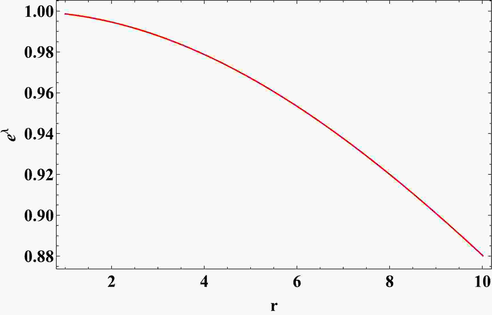
(28) The aforementioned results clearly indicate that there are no singularities in the inner solutions, thereby addressing the issue of a classical black hole's central singularity. For additional clarity, we plotted the variation of the metric potential
${\rm e}^{\lambda}$ with respect to the radial parameter r in Fig. 1.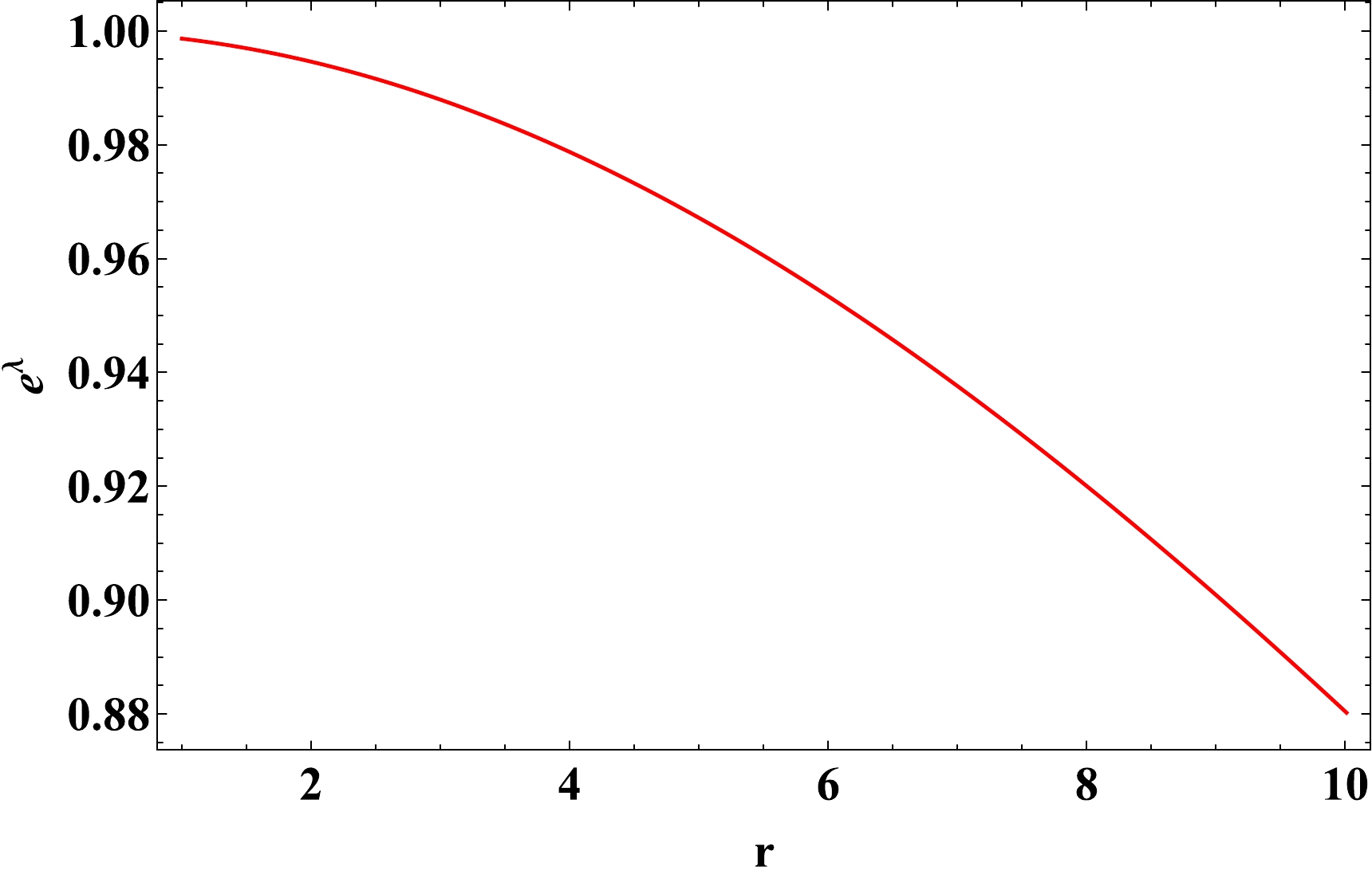
Figure 1. (color online) Variation in the metric potential (
$ e^{\lambda} $ ) with respect to the radial parameter r for$ \alpha=-4.5 $ ,$ \beta=3.4 $ ,$ \rho_c=0.001 $ .One can physically infer from the figure that there is no central singularity, and that the metric potential remains regular at
$ r = 0 $ , and it is finite and positive across the whole interior area. Additionally, the following equation can be used to determine the active gravitational mass of the internal region:$ \begin{equation} \mathcal{M(R)}=\int_0^{\mathcal{R}} 4 \pi r^2 \rho {\rm d}r =\frac{4}{3} \pi \mathcal{R}^3 \rho_c . \end{equation} $

(29) Where
$ \mathcal{R} $ represents the radius for the interior area and$ \rho_c $ denotes the critical density. -
The shell is made of ultra-relativistic stiff matter and abides by the EoS
$ p=\rho $ . Zel'dovich [45, 46] was the pioneer of the concept of this highly relativistic fluid, referred to as the stiff fluid, in relation to the cold baryonic universe. In the present context, this could potentially arise from thermal excitation with a very low chemical potential or from a maintained number density of gravitational quanta at absolute zero. Numerous researchers have extensively studied this type of fluid to explore various cosmological [47−49] and astrophysical [50−52] aspects. It should be noted that it is extremely challenging to solve the field equations in the non-vacuum area or shell. However, an analytical solution can be determined within the specifications of the thin shell limit, i.e.$0 < {\rm e}^{-\lambda(r)} \ll 1$ . We can argue that the interior area between the two space–times must be a thin shell, as suggested by Israel [53]. Moreover, in general, any parameter that is a function of r can be considered$\ll 1$ as$ r\to 0 $ . By considering this type of approximation, our field Eqs. (16)−(18) along with the Eqs. (19)−(21) reduce to:$ \begin{equation} \alpha \left(\frac{{\rm e}^{-\lambda} \lambda'(r)}{r}+\frac{1}{r^2}\right)=8 \pi \rho+ \frac{\beta}{2}(5 p+\rho), \end{equation} $

(30) $ \begin{equation} \alpha\left(\frac{-1}{r^2}\right)=8 \pi p+\frac{\beta}{2}(\rho-3 p), \end{equation} $

(31) $ \begin{equation} \alpha\left(\frac{-\lambda' \nu' {\rm e}^{-\lambda(r) }}{4}-\frac{{\rm e}^{-\lambda}\lambda'}{2r}\right)=8 \pi p+\frac{\beta}{2}(\rho-3 p). \end{equation} $

(32) Utilizing the Eqs. (30)−(32) we realize the two metric potential as
$ \begin{equation} {\rm e}^{-\lambda(r)}= \frac{2 (\beta +8 \pi ) \log (r)}{8 \pi -\beta }-C_2 , \end{equation} $

(33) $ \begin{equation} {\rm e}^{\nu(r)}= C_3 \left(r(\beta +8 \pi ) \right)^{\textstyle-\frac{32 \pi }{\beta +8 \pi }}. \end{equation} $

(34) Where
$ C_2 $ and$ C_3 $ denote integrating constants. Furthermore, by plugging the EoS$ p=\rho $ and using Eq. (34) into the energy conservation Eq. (23), we obtain the pressure/ matter density for the shell region as follows:$ \begin{equation} p(r)=\rho(r)= \rho_0 \left(8 \pi r-\beta r\right)^{\textstyle\frac{32 \pi }{8 \pi -\beta }}. \end{equation} $

(35) Where
$ \rho_0 $ denotes the constant of integration. Fig. 2 illustrates the variation of pressure or matter density. It can be seen that the shell's matter density monotonically increases towards its outer boundary. Given that the shell is composed of ultra-relativistic stiff fluid and the pressure or matter density increases monotonically towards the outer surface, we can physically interpret this as the concentration of stiff matter increasing towards the outer border as opposed to the internal region of the shell.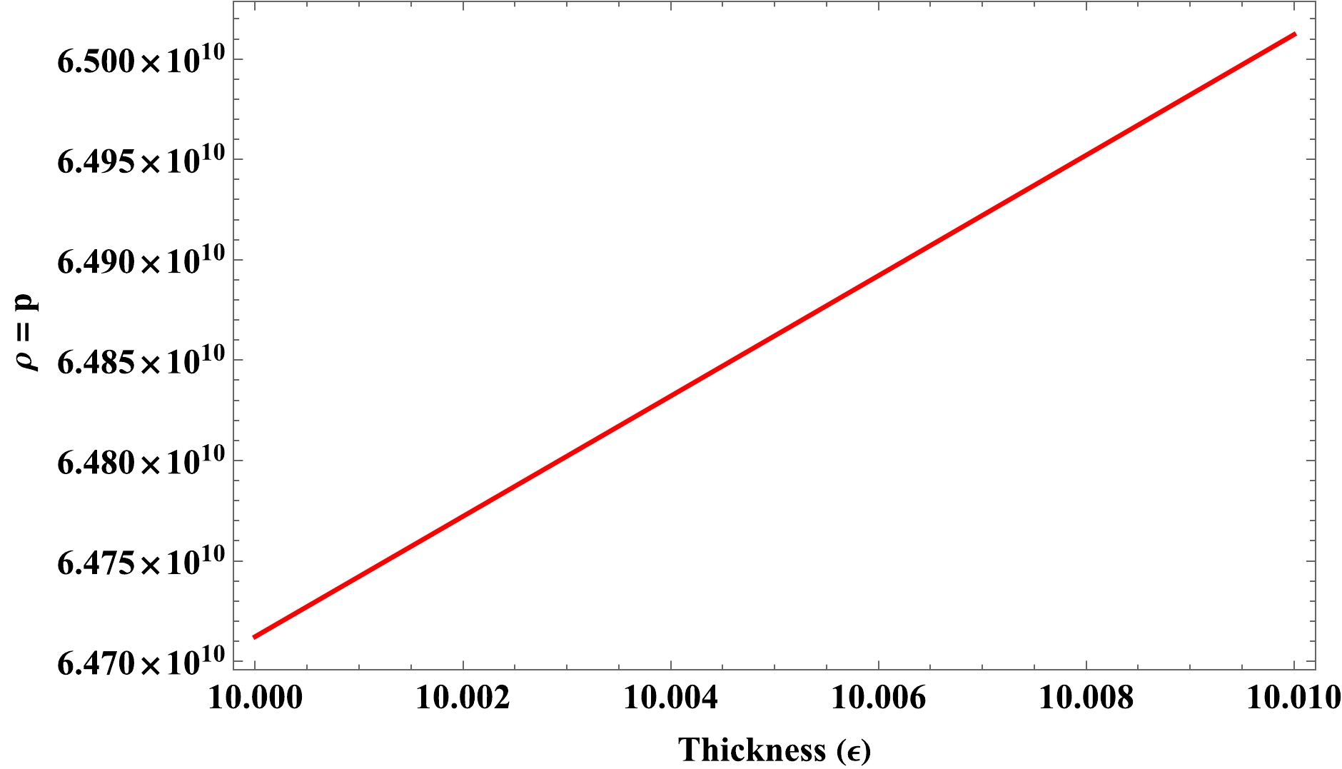
Figure 2. (color online) Variation in the pressure or matter density
$ p=\rho $ ($\textrm{km}^{-2}$ ) with respect to the thickness$\epsilon({\rm km})$ of the shell for$ \beta=3.4 $ ,$ \rho_0=1 $ . -
The EoS
$ p=\rho=0 $ is believed to be obeyed by the outside of a gravastar, indicating that the external portion of the shell is entirely vacuum. Thus, utilizing Eqs. (16)−(17) along with the Eqs. (19)−(20), we obtain$ \begin{equation} \lambda'+\nu'=0. \end{equation} $

(36) The line element for the outside region may be considered as the well-known Schwarzschild metric, which is provided by solution to Eq. (35) as follows:
$ \begin{equation} {\rm d}s^2=\left(1-\frac{2M}{r}\right){\rm d}t^2-\left(1-\frac{2M}{r}\right)^{-1} {\rm d}r^2-r^2 {\rm d}\Omega^2, \end{equation} $

(37) where
${\rm d}\Omega^2=({\rm d}\theta^2+{\rm sin}^2\theta {\rm d}\phi^2)$ and M denotes the total mass of the object. -
There are two junctions/interfaces in a gravastar configuration. Let us denote the interface between interior space–time and intermediate thin shell (at
$ r=R_1 $ ) by junction-I, and the interface between the intermediate thin shell and exterior space-time (at$ r=R_2 $ ) by junction-II. It is necessary that the metric functions at these interfaces must be continuous for any stable arrangement. We matched the metric functions at these borders to find the unknown constants of our current study such as$ C_1 $ ,$ C_2 $ , and$ C_3 $ , and we ultimately discovered the values of these constants.● Junction-I:
$ \begin{equation} \frac{2 (\beta +8 \pi ) \log R_1}{8 \pi -\beta }-C_2 = \frac{2 \rho_c(\beta -4 \pi ) R_1^2 }{3 \alpha }+1, \end{equation} $

(38) $ \begin{equation} C_3 \left(R_1(\beta +8 \pi ) \right)^{\textstyle-\frac{32 \pi }{\beta +8 \pi }}=C_1 \left[2 \rho_c (4 \pi -\beta ) R_1^2-3 \alpha\right]. \end{equation} $

(39) ● Junction-II:
$ \begin{equation} \frac{2 (\beta +8 \pi ) \log R_2}{8 \pi -\beta }-C_2 = 1-\frac{2 M}{R_2}, \end{equation} $

(40) $ \begin{equation} C_3 \left(R_2(\beta +8 \pi ) \right)^{\textstyle-\frac{32 \pi }{\beta +8 \pi }}=1-\frac{2M}{R_2}. \end{equation} $

(41) ● Obtained Constants:
$ \begin{equation} C_3=-\frac{(2 M-R_2) ((\beta +8 \pi ) R_2)^{\textstyle\frac{32 \pi }{\beta +8 \pi }}}{R_2}, \end{equation} $

(42) $ \begin{equation} C_2= \frac{2 (\beta +8 \pi ) \log (R_1)}{8 \pi -\beta }-\frac{2 \rho_c (\beta -4 \pi ) R_1^2}{3 \alpha }-1, \end{equation} $

(43) $ \begin{equation} C_1= \frac{(2 M-R_2) ((\beta +8 \pi ) R_1)^{\textstyle-\frac{32 \pi }{\beta +8 \pi }} ((\beta +8 \pi ) R_2)^{\textstyle\frac{32 \pi }{\beta +8 \pi }}}{R_2 \left(3 \alpha +2 \beta \rho_c r^2-8 \pi \rho_c R_1^2\right)}. \end{equation} $

(44) To find the numerical values of constants
$ C_1 $ ,$ C_2 $ , and$ C_3 $ , we considered the astrophysical object PSR J1416- 2230 [54] with$M=1.97~M_{\odot}$ , internal radius$ R_1=10 $ , and exterior radius$ R_2=10.01 $ . Additionally, by adjusting a series of values for the model parameters α and β, we have determined a set of numerical values of$ C_1 $ ,$ C_2 $ , and$ C_3 $ which is listed in Table 1.α β $ C_1 $ 

$ C_2 $ 

$ C_3 $ 

$ -4.5 $ 

$ 3.4 $ 

$ 0.0396871 $ 

$ 4.91029 $ 

$ 2.72477\times10^8 $ 

$ -4.6 $ 

$ 3.3 $ 

$ 0.0388762 $ 

$ 4.86301 $ 

$ 2.88649\times10^8 $ 

$ -4.7 $ 

$ 3.2 $ 

$ 0.0380979 $ 

$ 4.81611 $ 

$ 3.05892\times10^8 $ 

$ -4.8 $ 

$ 3.1 $ 

$ 0.0373501 $ 

$ 4.76958 $ 

$ 3.24284\times 10^8 $ 

$ -4.9 $ 

$ 3.0 $ 

$ 0.0366311 $ 

$ 4.72344 $ 

$ 3.4391\times 10^8 $ 

Table 1. Different numerical values of constants for PSR J1416-223 assuming
$ R_1=10 \, $ km and$ R_2=10.01 $ km.In relation to the provided numerical solutions of constants for some specific parameter choices given above, we will discuss the parameter space of our solution. Some associated issues to consider are as follows:
1. For particular choices of
$M,~ R_1,~ R_2$ , will we always obtain a singular free solution?2. If one varies the model parameter, then will the results be unique or not?
We provide some arguments to answer these concerns: In the current study, we selected values for a number of factors to examine the physical behavior of a gravastar. It will provide a unique solution for a given value of M,
$ R_1 $ , and$ R_2 $ , but we selected these values to satisfy ratios$ \dfrac{2M}{R_1}<1,\dfrac{2M}{R_2}<1 $ for a stable gravastar model. Furthermore, some other criteria, such as the surface redshift$ \mathcal{Z_\mathrm{s}}<2 $ and square of the speed of sound($ v_s^2 $ ), must satisfy the inequality$ 0<v_s^2<1 $ . Additionally, for avoiding central singularity, we should maintain$ \dfrac{2(\beta-4 \pi) \rho_c r^2 }{3 \alpha } +1 \neq 0 $ . Moreover, we considered$ \rho_0=1 $ and$ \rho_c=0.001 $ to maintain$ \rho_0>>\rho_c $ . We are free to choose any M,$ R_1 $ , and$ R_2 $ combination that can provide the same findings as those presented in this research as long as the aforementioned requirements are valid. -
It is established that a gravastar is divided into three regions, namely the interior (I), intermediate thin shell (II), and exterior (III). This shell serves to connect the internal and outer regions, thus playing a crucial role in the construction of a gravastar. According to the basic junction condition, regions I and III must smoothly meet at the junction. Although the metric coefficients are continuous at the junction surface, their derivatives may not be. To calculate the surface stresses at the junction, we will now apply the Darmois–Israel [55, 56] condition. Lanczos equation [57−60] provides the intrinsic surface stress–energy tensor
$ S_{ij} $ in the following manner:$ \begin{align} S_{ij}=-\frac{1}{8 \pi}(k_{ij}-\delta_{ij} k_{\gamma \gamma}). \end{align} $

(45) In the aforementioned expression,
$ k_{ij}=K^{+}_{ij}-K^{-}_{ij} $ denotes the discontinuity in some second fundamental expression. Where the second fundamental expression is as follows:$ \begin{equation} K^{\pm}_{ij}=-n^{\pm}_{\sigma} \left( \frac{\partial x_{\sigma}}{\partial \phi^{i} \partial \phi^{j}} +\Gamma^{l}_{km} \frac{\partial x^l}{\partial \phi^{i}} \frac{\partial x^m}{\partial \phi^{j}} \right), \end{equation} $

(46) where
$ \phi^{i} $ denotes the intrinsic co-ordinate in the shell area, and$ n^{\pm} $ represents the two-sided unit normal to the surface, which can be expressed as$ \begin{equation} n^{\pm}=\pm \left|g^{lm} \frac{\partial f}{\partial x^{l}} \frac{\partial f}{\partial x^{m}} \right|^{-1/2} \frac{\partial f}{\partial x^{\sigma}}, \end{equation} $

(47) with
$ n^{\gamma} n_{\gamma} =1 $ . Utilizing the Lanczos method [57], the surface energy tensor can be expressed as$S_{ij}={\rm diag}(-\sum, P)$ , where the surface energy density and surface pressure are denoted by$ \sum $ and P, respectively, and are defined as follows:$ \begin{equation} \sum=-\frac{1}{4 \pi \mathcal{R}} \left[\sqrt {{\rm e}^{-\lambda}}\right]^+_-, \end{equation} $

(48) $ \begin{equation} P=-\frac{\sum}{2}+\frac{1}{16 \pi}\left[\frac{({\rm e}^{-\lambda})^{\prime}}{\sqrt {{\rm e}^{-\lambda}}}\right]^+_-, \end{equation} $

(49) $ \begin{equation} \text{Also the EoS}\,(\omega)=\frac{P}{\sum}. \end{equation} $

(50) Specifically,
$ - $ and$ + $ denote the interior space–time and Schwarzschild space–time, respectively. Calculating Eqs. (48)−(50), we obtain the expression of the above quantities as$ \begin{equation} \sum=\left(-\frac{1}{4 \pi R}\right)\left(\sqrt{1-\frac{2 M}{R}}-\sqrt{\frac{2 (\beta -4 \pi ) \rho \text{ c} R^2}{3 \alpha }+1}\right), \end{equation} $

(51) $ \begin{aligned}[b] P=&\frac{1}{16 \pi }\left(\dfrac{2 M}{R^2 \sqrt{1-\dfrac{2 M}{R}}}-\frac{4 (\beta -4 \pi ) \rho_c R}{3 \alpha \sqrt{\dfrac{2 (\beta -4 \pi ) \rho_c R^2}{3 \alpha }+1}}\right)\\&-\frac{1}{2} \left(-\frac{1}{4 \pi R}\right)\left(\sqrt{1-\frac{2 M}{R}}-\sqrt{\frac{2 (\beta -4 \pi ) \rho_c R^2}{3 \alpha }+1}\right), \end{aligned} $

(52) $ \omega=\frac{\dfrac{1}{16 \pi }\left(\dfrac{2 M}{R^2 \sqrt{1-\dfrac{2 M}{R}}}+\dfrac{4 (4 \pi -\beta ) \rho_c R}{\alpha \sqrt{\dfrac{6 (\beta -4 \pi ) \rho_c R^2}{\alpha }+9}}\right)}{\left(-\dfrac{1}{4 \pi R}\right)\left(\sqrt{1-\dfrac{2 M}{R}}-\sqrt{\dfrac{2 (\beta -4 \pi ) \rho_c R^2}{3 \alpha }+1}\right)}-\frac{1}{2}. $

(53) There exists a set of criteria known as energy conditions that must be satisfied for a geometric structure to be physically viable. These widely recognized energy conditions are as follows:
1. NEC:
$ \sum+P> 0 $ ,2. WEC:
$ \sum> 0 $ ,$ \sum+P>0 $ ,3. SEC:
$ \sum+P> 0 $ ,$ \sum+3P> 0 $ ,4. DEC:
$ \sum > 0,\sum \pm P> 0 $ .The proposed model is physically feasible if these energy conditions are met. We are examining whether the null energy condition, which ensures the presence of either ordinary or exotic matter in the thin shell, is satisfied. In this context, it is worth noting that violation of null energy conditions (NEC) results in violation of other energy conditions. It is illustrated in Fig. 3 that the NEC is satisfied over a range of model parameter values throughout the entire region.
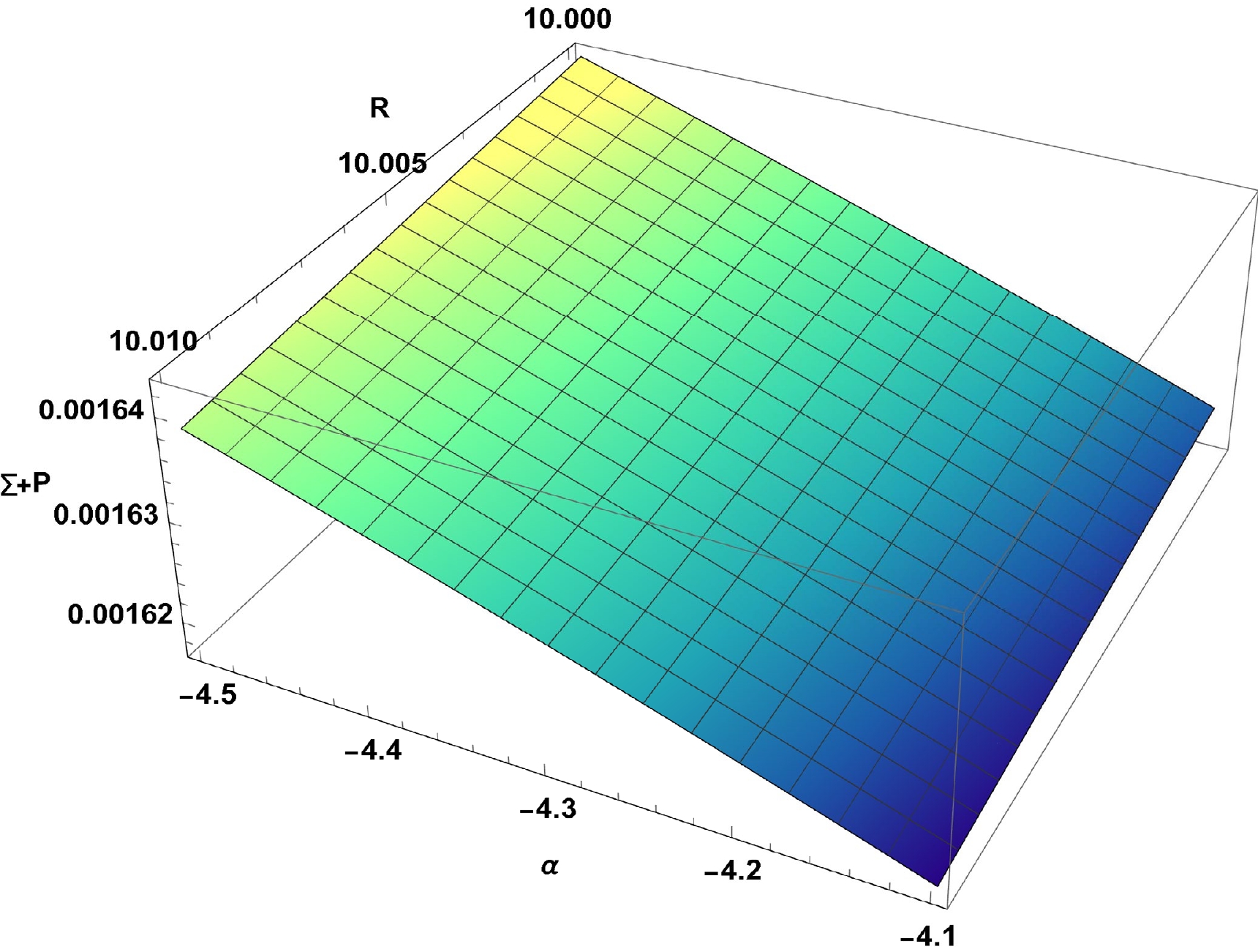
Figure 3. (color online) Evolution of NEC (
$ \sum+P $ ) by varying model parameter α.Furthermore, we have plotted the variation in surface energy density with respect to the thickness parameter (
$ \epsilon $ ) in Fig. 4, which shows that the surface energy density monotonically decreases toward the boundary of the shell. Hene, the mass of the thin shell can be easily determined using the equation for the surface energy density as follows: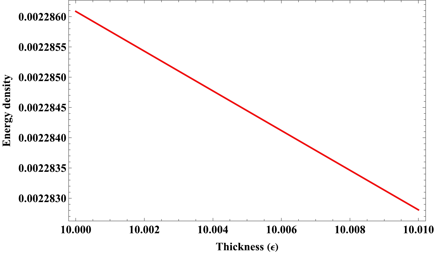
Figure 4. (color online) Variation in the surface energy density (
$ \sum $ ) with respect to thickness$ \epsilon(\text{in km}) $ for$ \alpha=-4.5, \beta=3.4 $ .$ \begin{eqnarray} m_s= 4\pi R^2 \sum = -R\left(\sqrt{1-\frac{2 M}{R}}-\sqrt{\frac{2 (\beta -4 \pi ) \rho_c R^2}{3 \alpha }+1}\right). \end{eqnarray} $

(54) To determine the real value of shell mass, we use inequality
$ m_s>0 $ to obtain the upper bound of the radius as$R < \left[\dfrac{3 M \alpha}{\rho_c (4 \pi- \beta)}\right]^\frac{1}{3}.$ Thus, we obtain the limiting value on the radius as$ \begin{equation} 2M<R<\left[\frac{3 M \alpha}{\rho_c (4 \pi- \beta)}\right]^{1/3}. \end{equation} $

(55) -
According to Mazur and Mottola's hypotheses [1, 2], the stiff fluid of the shell is positioned between the meeting of two space–times. The length of the shell ranges from
$ R_1=R $ (which is the phase barrier between the interior area and intermediate thin shell) up to$ R_2=R+\epsilon $ (which is the phase border between the exterior space–time and intermediate thin shell). Hence, by using the following formula, we can determine the required length or proper thickness of the shell, as well as the proper thickness between these two interfaces:$ \begin{aligned}[b] l =&\int^{R+\epsilon}_{R} \sqrt{{\rm e}^{\lambda}}{\rm d}r, \\ =&\int^{R+\epsilon}_{R} \sqrt{\frac{\beta -8 \pi }{(8 \pi -\beta ) C_2-2 (\beta +8 \pi ) \log (r)}} \, {\rm d}r,\\ =&\left[-{\rm e}^{\textstyle-\frac{(\beta -8 \pi ) C_2}{2 (\beta +8 \pi )}}\sqrt{\frac{\pi (\beta -8 \pi )}{2 (\beta +8 \pi )}} \text{Erf}\sqrt{\frac{(8 \pi -\beta ) C_2}{2 (\beta +8 \pi )}-\log (r)} \right]_{R}^{R+\epsilon} \end{aligned} . $

(56) The variation in the proper length with respect to the thickness parameter
$ \epsilon $ is provided in Fig. 5. The figure demonstrates that the proper length increases monotonically as shell thickness increases.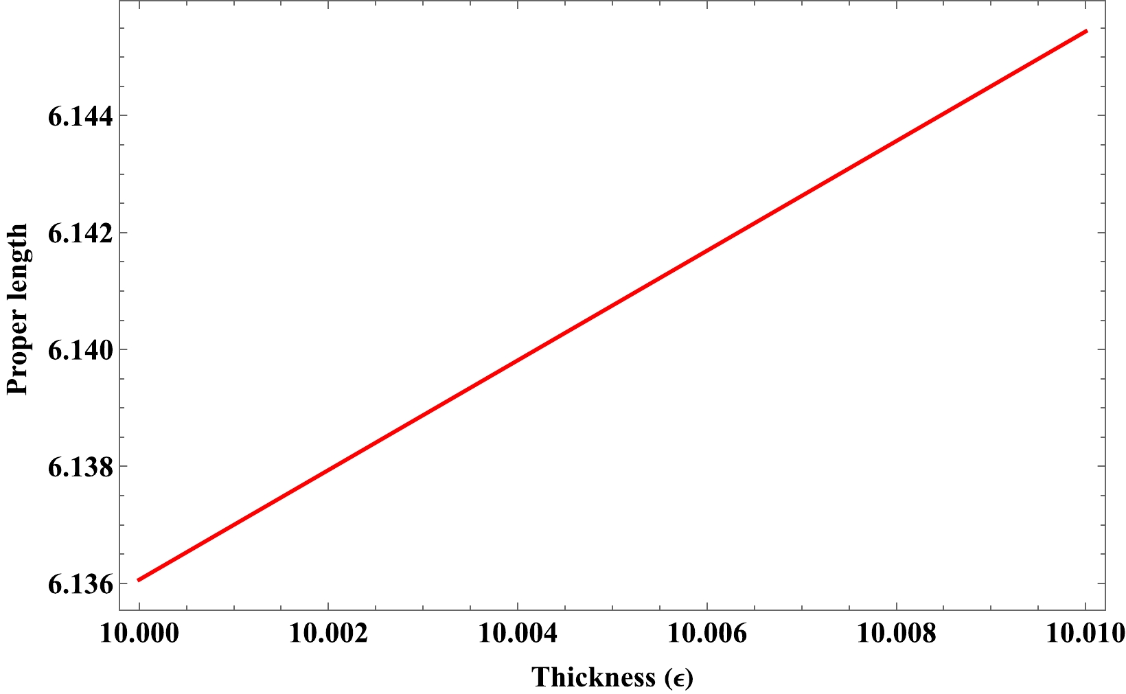
Figure 5. (color online) Variation in the proper length (l) with respect to thickness
$ \epsilon(\text{in km}) $ for$ \alpha=-4.5 $ and$ \beta=3.4 $ . -
The energy of the shell can be calculated by the formula below as follows:
$ \begin{aligned}[b] E=&\int^{R+\epsilon}_R 4\pi r^2 \rho \, {\rm d}r, \\ E=&\int^{R+\epsilon}_R 4\pi r^2 \rho_0 \left(8 \pi r-\beta r\right)^{\textstyle\frac{32 \pi }{8 \pi -\beta }} \,\, {\rm d}r, \\ E =&\frac{4 \pi \rho_0 r^2 ((8 \pi -\beta ) r)^{\textstyle\frac{32 \pi }{8 \pi -\beta }+1}}{56 \pi -3 \beta }. \end{aligned} $

(57) The variation in the shell energy is illustrated in Fig. 6. In this graph, it can be observed that the energy increases as the shell's thickness increases. The fluctuation of energy is comparable to the fluctuation in matter density. It satisfies the requirement that the energy of the shell must be increased as the radial distance increases.
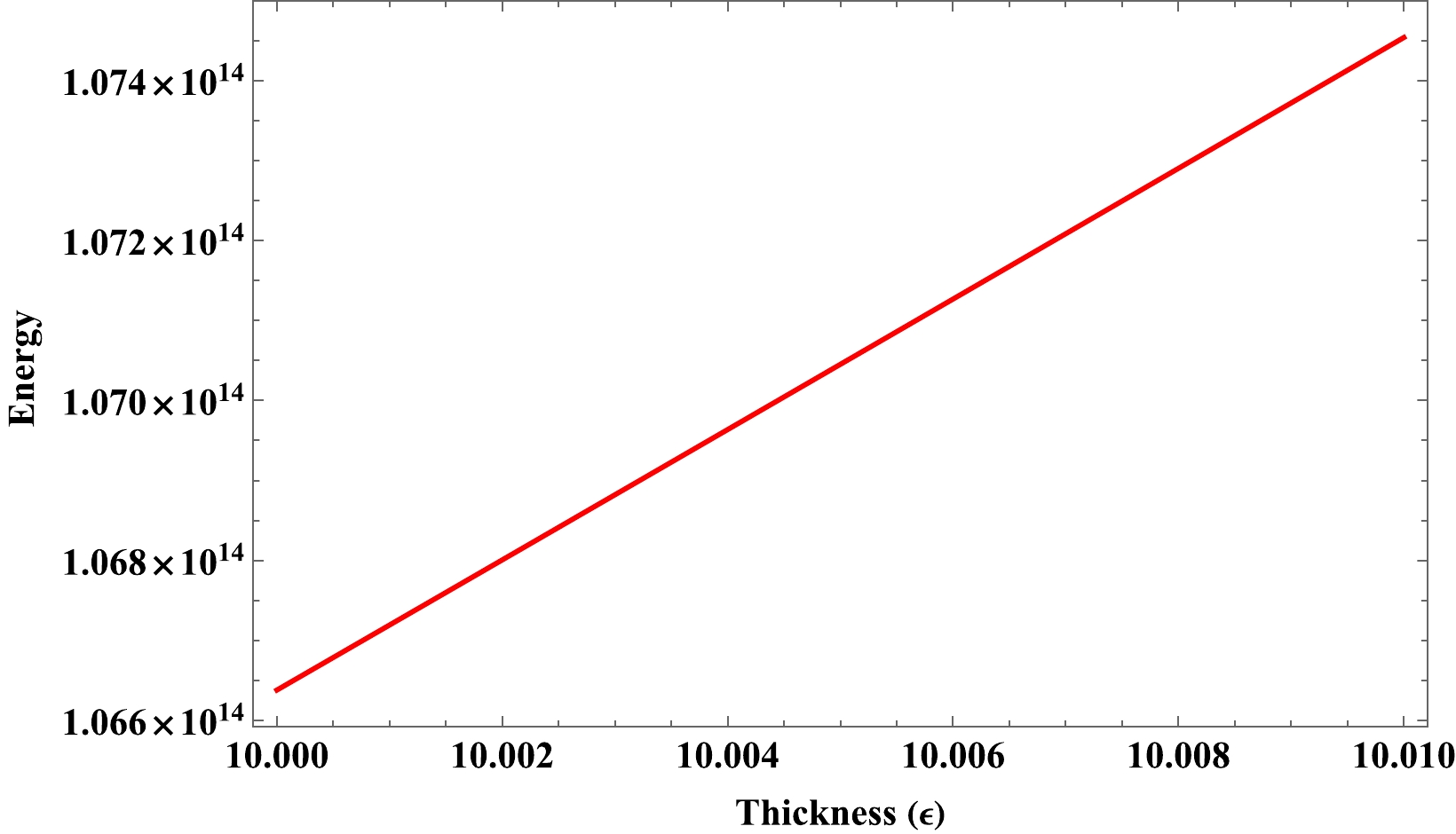
Figure 6. (color online) Variation in energy
$ (E) $ with respect to thickness$ \epsilon(\text{in km}) $ for$ \alpha=-4.5 $ and$ \beta=3.4 $ . -
The stable configuration for a single condensate area is zero entropy density, which is present in a gravastar's innermost region. Entropy on the intermediate thin shell can be calculated using the formula presented by Mazur and Mottola [1, 2] as follows:
$ \begin{equation} \mathcal{S}= \int^{R+\epsilon}_{R} 4 \pi r^2 s(r) \sqrt{{e}^{\lambda}} {\rm d}r, \end{equation} $

(58) where the entropy density at local temperature
$ T(R) $ is provided by expression$ s(r)=\dfrac{\gamma^2 K_{B}^2 T(R)}{4 \pi \hbar^2 }= \gamma \sqrt{p/{2\pi}} $ , where γ denotes the dimensionless parameter. In this study, we considered geometrical units, i.e.,$ G=c=1 $ as well as Planckian units$ K_{B}=1, \hbar =1 $ . Our estimates of the entropy of the thin shell are limited to the second-order term of the thickness parameter, i.e., order$ \epsilon^2 $ , using Taylor series approximation. Ultimately, we calculated the intermediate thin shell's entropy as follows:$ \begin{aligned}[b] \mathcal{S}=& 2 \sqrt{2 \pi } \gamma r^2 \epsilon \sqrt{\frac{(\beta -8 \pi ) \rho_0 (8 \pi r-\beta r)^{\textstyle\frac{32 \pi }{8 \pi -\beta }}}{(8 \pi -\beta ) C_2-2 (\beta +8 \pi ) \log (r)}}\,\,\\&+ \frac{\epsilon ^2 \left(2 \sqrt{2 \pi } \gamma r ((8 \pi -\beta ) (\beta -2 \beta C_2+8 \pi (4 C_2+1))-4 (16 \pi -\beta ) (\beta +8 \pi ) \log (r)) \sqrt{\dfrac{(\beta -8 \pi ) \rho_0 ((8 \pi -\beta ) r)^{\textstyle-\frac{32 \pi }{\beta -8 \pi }}}{(8 \pi -\beta ) C_2-2 (\beta +8 \pi ) \log (r)}}\right)}{2 \left((\beta -8 \pi )^2 C_2+2 \left(\beta ^2-64 \pi ^2\right) \log (r)\right)}. \end{aligned} $ 
(59) Figure 7 depicts the evolution of the shell entropy, which shows the growing behavior of the shell entropy with respect to thickness (
$ \epsilon $ ). Another prerequisite for a stable gravastar configuration is that entropy should reach its maximum value on the surface, as demonstrated in our analysis.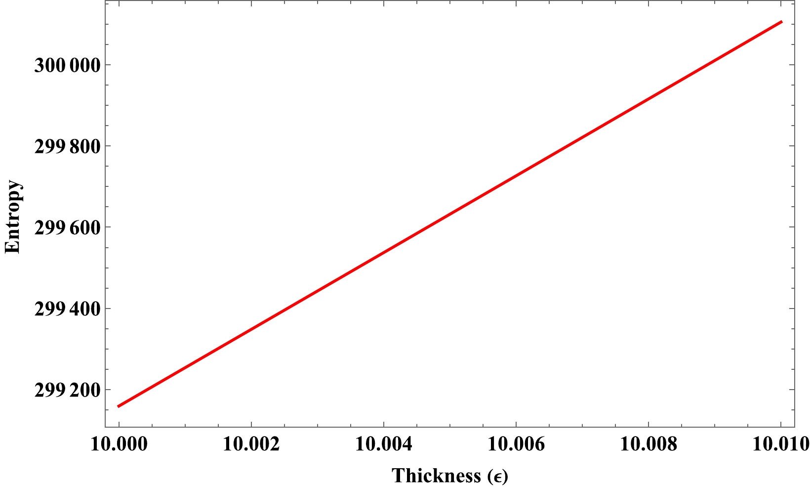
Figure 7. (color online) Variation in entropy (
$ \mathcal{S} $ ) with respect to thickness$ \epsilon(\text{in km}) $ for$ \beta=3.4 $ ,$ \alpha=-4.5 $ . -
In this section, we investigate the stability of the thin shell gravastar model by analyzing certain physical parameters.
-
Recent observational data appear to indicate that the cosmos is expanding more quickly than earlier [3−5]. If general relativity is considered as the correct theory of gravity, characterizing the behavior of the universe on a large scale, then the energy density and pressure of the cosmos should violate the strong energy condition. The stable or unstable configuration of gravastars can be analyzed based on the nature of η, where η is an effective parameter that can be interpreted as the square of the speed of sound i.e.
$ \eta=v_s^2 $ [27, 61]. For a stable system, η should satisfy$ 0<\eta\leq 1 $ . As is clear, the speed of sound should not exceed the speed of light. However, this restriction may not be met on the surface layer when testing the stability of a gravastar. The square of the speed of sound is defined as follows:$ \begin{equation} \eta=v_s^2=\frac{P^{\prime}}{\sum'}. \end{equation} $

(60) Where ' denotes the derivative with respect to the radial coordinate. Hence, by using (51, 52), we examine the parameter's sign to determine the stability of gravastar configurations. We utilize the graphical behavior, as the mathematical expression of η is complicated.
From Fig. 8, it can be observed that the effective parameter η satisfies inequality
$ 0<\eta\leq 1 $ throughout the entire shell region. Here, we varied the model parameter α and observed that for each value of α, our model behaves physically stable. Another key observation worth mentioning is that as the value of α increases, parameter$ \eta \to 1 $ . Hence, as the model parameter value increaes, our proposed gravastar model approaches the unstable condition.
Figure 8. (color online) Variation in η with respect to thickness
$ \epsilon(\text{in km}) $ for different values of α. -
The study of a gravastar's surface redshift is one of the most basic ways to understand the stability and detection of the object. Specifically, formula
$Z_s={\Delta \lambda}/{\lambda_e} ={\lambda_0}/{\lambda_e}$ can be used for determining the gravitational surface redshift of a gravastar, where$ \lambda_0 $ and$ \lambda_e $ denote the wavelength detected by the observer and emitted from the source. Buchdahl [62, 63] proposed that the value of surface redshift should not be more than 2 for an isotropic, stable, and perfect fluid distribution. However, Ivanov [64] claimed that for anisotropic fluid dispersion, it might be as high as$ 3.84 $ . Furthermore, Barraco and Hamity [65] showed that for an isotropic fluid distribution,$ Z_s\leq 2 $ holds when the cosmological constant is absent. Bohmer and Harko [66] showed that in the presence of the anisotropic star's cosmological constant,$ Z_s \leq 5 $ . In our case, we obtained the surface redshift by the following formula:$ \begin{equation} Z_s=-1+\frac{1}{\sqrt{g_{tt}}}=\frac{1}{\sqrt{C_3 ((\beta +8 \pi ) r)^{\textstyle-\frac{32 \pi }{\beta +8 \pi }}}}-1 . \end{equation} $

(61) The graphical analysis of
$ Z_s $ is provided in Fig. 9. We varied the model parameter α and β for analyzing the maximum possibility case of$ Z_s $ , and in each case, it is noticed that$ Z_s<1 $ . Consequently, we can assert that the current gravastar model is physically stable and appropriate in the$ f(Q, T) $ framework.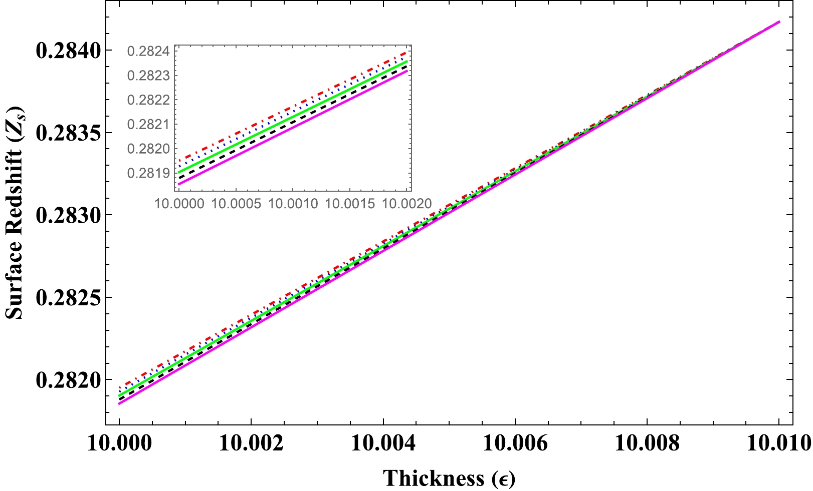
Figure 9. (color online) Variation in
$ Z_s $ with respect to thickness$ \epsilon(\text{in km}) $ for different values of model parameter$ \alpha \,\text{and} \, \beta $ . Red Dotdashed ($ \alpha=-4.1, \beta=3.9 $ ), Blue Dotted ($\alpha=-4.4, $ $ \beta=3.6$ ), Green Tan ($ \alpha=-4.7, \beta=3.3 $ ), Black Dashed ($\alpha=-5.0, $ $ \beta=3.0$ ), and Magenta Thickness ($ \alpha=-5.3, \beta=2.7 $ ). -
Each quasi-black hole (QBH) candidate must be stable to constitute a physically feasible endpoint of gravitational collapse [67]. To verify the stability of the current investigation of gravastar in
$ f(Q,T) $ gravity, we used the entropy maximization method recommended by Mazur and Mottola [1, 2]. Given that the shell region is only the non-vacuum region with stiff fluid and contains the positive heat capacity, the solution should be thermodynamically stable. To check the stability, we will use the entropy maximization technique in the shell region. To maximize the entropy function, the first variation of the entropy function should initially vanish at the boundaries of the shell, i.e.,$ \delta \mathcal{S}=0 $ at$ r=R_1 $ and$ r=R_2 $ . We check the nature of the second derivative, i.e., of$ \delta^2 \mathcal{S} $ , based on its sign for all the variations in$ M(r) $ . The entropy function is as follows:$ \begin{equation} \mathcal{S}=\frac{\gamma k_B}{ \hbar G} \int_{R_1}^{R_2} r {\rm d} r\left(2\frac{ {\rm d} M}{{\rm d} r}\right)^{{1}/{2}} \frac{1}{\sqrt{1-\frac{2 M(r)}{r}}}. \end{equation} $

(62) In the context of a hydrodynamic treatment, thermodynamic stability is a necessary and sufficient condition for the dynamic stability of a static, spherically symmetric solution to the field problem. The second derivative of the entropy function is as follows:
$\begin{aligned}[b] \delta^2 \mathcal{S}=&\frac{\gamma k_B}{\hbar G} \int_{R_1}^{R_2} r {\rm d} r\left(2 \frac{{\rm d} M}{{\rm d} r}\right)^{-{3}/{2}} \left(1-\frac{2 M}{r}\right)^{-{1}/{2}}\\ &\left\{-\left[\frac{{\rm d}(\delta M)}{{\rm d} r}\right]^2+2 \frac{(\delta M)^2}{r^2 \left(1-\dfrac{2 M}{r}\right)^2} \frac{{\rm d} M}{{\rm d} r}\left(1+2 \frac{{\rm d} M}{{\rm d} r}\right)\right\}. \end{aligned} $

(63) With the aid of Eqs. (33), (37), and (43), we determined the functional value of
$ M(r) $ as follows:$ \begin{equation} \begin{gathered} M(r)=\frac{r \left(3 \alpha (\beta +8 \pi ) \ln (\frac{R_1}{r})+\left(\beta ^2-12 \pi \beta +32 \pi ^2\right) \rho_c R_1^2\right)}{3 \alpha (8 \pi -\beta )}. \end{gathered} \end{equation} $

(64) Additionally, if we consider the linear combination of
$ M(r) $ as$ \delta M=\chi_0 \psi $ , where ψ vanishes at boundaries$ R_1 $ and$ R_2 $ , then by partially integrating Eq. (63) using the diminishing of the variation$ \delta M $ , we obtain:$ \begin{equation} \delta^2 \mathcal{S}=-\frac{\gamma k_B}{\hbar G} \int_{R_1}^{R_2} \frac{r {\rm d} r} {\sqrt{\left(1-\dfrac{2 M}{r}\right)}}\left(2 \frac{{\rm d} m}{{\rm d} r}\right)^{-{3}/{2}} \chi_0^2\left(\frac{{\rm d} \psi}{{\rm d} r}\right)^2<0 . \end{equation} $

(65) It is evident from the above expression that for any radial variations that vanish at the endpoints of the shell's boundaries, the entropy function in
$ f(Q, T) $ gravity reaches its maximum value. We can therefore conclude that a perturbation in the fluid of a gravastar's intermediate shell area results in a decrease in entropy in region II, which suggests that our solutions are stable against minor perturbations with the specified endpoints. Essentially, the stability of a gravastar is not compromised by the effects of$ f(Q,T) $ gravity. -
Based on the model proposed by Mazur–Mottola [1, 2] within the context of general relativity, we developed a unique stellar model of a gravastar under the theory of
$ f(Q, T) $ gravity. The model comprises three distinct regions: the interior region, intermediate thin shell, and exterior space-time, each with a different EoS. The interior region is entirely composed of dark energy as hypothesized by [1, 2]. The following are some crucial characteristics of a gravastar:● Interior Region : Using the EoS (25), we derived two non-singular metric potentials (27, 28) from the described field equation in
$ f(Q,T) $ gravity. The metric potentials are finite and remain positive throughout the entire interior region. This confirms that our proposed gravastar model in$ f(Q,T) $ gravity is devoid of the concept of central singularity in CBH.● Intermediate thin shell: We estimated the metric potentials in the region of the shell by using the thin shell approximation. Equations (33) and (34) indicate that two metric potentials remain finite as well as positive throughout the entire shell.
- Pressure or matter density: In addition to using the energy conservation Eq. (23), we derived the pressure or matter density (35) in the shell. Figure 2 represents the variation in the pressure or matter density with respect to the thickness parameter (
$ \epsilon $ ). One can observe that the matter density of the shell is monotonically increasing towards the shell's outer boundary. Given that the shell is composed of ultra-relativistic stiff fluid, and considering the pressure or matter density is monotonically increasing toward the outer surface, we can physically interpret that the concentration of stiff matter is greater toward the outer border rather than the shell's internal region. Consequently, the shell's outer boundary becomes denser than the interior border.● Junction Condition and EoS : We consider the junction condition for the formation of a thin shell between the interior and external space–times. We analyze the variation in surface energy density with respect to the thickness parameter (
$ \epsilon $ ) using the Darmois–Israel junction condition, as shown in Fig. 4. The surface energy density increases towards the outer boundary of the shell. Furthermore, in Fig. 3, we verify that the NEC is satisfied over a range of model parameter values throughout the entire shell. It confirms the presence of ordinary or exotic matter in the shell. Additionally we obtain the limiting value of radius (55) using the concept of determining the real value of shell mass.● Physical Features of the Model: Using the geometrical quantity of the intermediate thin shell, we analyzed certain physical properties of the thin shell.
- Proper length: The variation in the proper length with respect to the thickness parameter
$ \epsilon $ is provided in Fig. 5 and in Eq. (56). The figure demonstrates that the appropriate length increases monotonically as shell thickness increases. This monotonically increasing behavior of proper length of gravastar is similar to the study which was conducted in modified gravity [20, 21].- Energy : The variation of the shell energy is illustrated in Fig. 6. In this graph, it can be observed that the energy increases as the shell's thickness increases. The fluctuation of energy is comparable to the fluctuation in matter density. It satisfies the requirement that the energy of the shell increases as the radial distance increases.
- Entropy : Figure 7 depicts the evolution of the shell entropy, which shows the growing behavior of the shell entropy with respect to thickness (
$ \epsilon $ ). Another acceptable condition is that entropy should reach its greatest value on the surface for a stable gravastar configuration, which is demonstrated in our analysis. To compare the energy and entropy of a gravastar model with those reported in a previous study [34], one can observe that the energy and entropy should reach their maximum values at the boundary of the shell, a condition that is met in our study● Stability of stellar model: Finally, we validated the stability of our proposed stellar model through the study of Herrera's cracking concept and the surface redshift analysis method. Subsequently, we employed the entropy maximization technique to assess the stability of a gravastar.
- Herrera's cracking concept: We analyzed the stability of a gravastar based on the nature of the effective parameter η. In Fig. 8, it is clear that for each value of α, the square of the speed of the sound remains positive and does not exceed 1. Moreover, we can observe that for increasing the value of α parameter, the model approaches instability.
- Surface Redshift: Lastly, we used surface redshift analysis to verify the stability of our recently suggested model. The surface redshift (
$ Z_s $ ) for any physically stable star arrangement should always be smaller than 2. By varying the model parameter β, we plotted the surface redshift with respect to the thickness parameter ($ \epsilon $ ), which is illustrated in Fig. 9. In each case,$ Z_s<1 $ . It demonstrates that our suggested model is stable under$ f(Q, T) $ gravity.- Entropy Maximization : Here, we utilized the entropy maximization technique to verify the stability of a gravastar system. To maximize the entropy function, the first variation of the entropy function is initially set to zero at the boundaries of the shell, i.e.,
$ \delta \mathcal{S}=0 $ at$ r=R_1 $ and$ r=R_2 $ . Subsequently, we checked the nature of the second derivative, i.e., of$ \delta^2 \mathcal{S} $ , by its sign for all the variations in$ M(r) $ . Equation (65) considers a negative value, which represents that the entropy attains its maximum value for all variations of the radial parameter. This further indicates the stability of our gravastar model in$ f(Q, T) $ gravity. One can verify the stability of the gravastar model using the entropy maximization technique in [1, 34].We conclude that a gravastar might exist within the constraints of
$ f(Q, T) $ gravity. Compared to previous studies on gravastars, we extended the thin shell approximation to the second order, which offers a more accurate analytical solution for determining the physical parameters of the shell. Additionally, we employed Herrera's cracking concept as a new technique to verify the stability of our proposed model in$ f(Q,T) $ gravity. We can conclude that the$ f(Q, T) $ theory of gravity was effectively used in the current study on a gravastar, as demonstrated by our findings. The issues associated with the event horizon and central singularity of a black hole are promptly addressed by a set of physically plausible, non-singular gravastar solutions.Data availability There are no new data associated with this article.
-
We are very grateful to the honorable referees and the editor for their insightful suggestions, which significantly improved our research quality and presentation.
Thin-shell gravastar model in f(Q, T) gravity
- Received Date: 2023-05-03
- Available Online: 2023-09-15
Abstract: In the last few decades, gravastars have been proposed as an alternative to black holes. The stability of a gravastar has been examined in many modified theories of gravity along with Einstein's GR. The


 DownLoad: