


 Abstract
 HTML
HTML Reference
 Related
 PDF
PDF


-
Inspired by the renowned concept of fermion-boson duality and the recently proposed fermion-bit correspondence [1, 2], we propose a map between nucleons bound in nuclei and Ising spins in the Ising model called the "SRC-bit map," where SRC is an abbreviation of "short-range correlation." A brief introduction to these sorts of maps will be presented presently.
The fermion-boson duality shows the equivalence of fermionic and bosonic particle systems; it stems from the following question — can bosons and fermions transform into each other? It is possible in supersymmetry, which is a spacetime symmetry between two basic classes of particles: bosons, which have an integer-valued spin and follow Bose-Einstein statistics, and fermions, which have a half-integer-valued spin and follow Fermi-Dirac statistics. In supersymmetry, each particle from one class would have an associated particle in the other, known as its superpartner. As one of the strongest candidates for physics beyond the Standard Model, supersymmetry has yet to be tested by high energy experiments. However, in low-dimensional non-relativistic systems, the equivalence of bosonic and fermionic systems was reported long ago [1, 3−11]. Massless boson and fermion theories in
$ 1+1 $ -dimensional Minkowski and curved space-time have been proved to be equivalent [12, 13]. Because the spin-statistics relation is based on relativity, a non-relativistic system can escape the spin-statistics relation, such that the boson can have spin while the fermion is spinless. The relation between a spin-bearing boson and a spinless fermion may shed light on the general properties of boson-fermion duality.A fermion-bit map is proposed based on the equivalence between the two formulations for describing fermions and Ising spins, as they could have the identical expectation values of products of observables. In the case of fermions, the observables are occupation numbers
$ n(x) $ , which take values 0 or 1. For$ n(x)=1 $ a fermion is present at x, while for$ n(x)=0 $ no fermion is located in x. In the case of Ising spins,$ s(x) $ can take the values$ \pm 1 $ , which can be understood as the magnetic dipole moments of atomic "spins" in ferromagnetism. A relation between occupation numbers and Ising spins can be readily established,$ n(x)= (s(x)+1)/2 $ . Based on these simple observations, a map between fermions and Ising models has been proposed [14, 15]. Since Ising spins can be associated with bits of information, this map has been termed the "fermion-bit map."Inspired by these relations, we propose a new mapping between nucleons and Ising spins. One may think of the stable nucleus as a tight ball of neutrons and protons (collectively called nucleons), held together by the strong nuclear force. This basic picture worked very well until deep inelastic scattering (DIS) led to the discovery that nucleons are made of quarks. However, due to the small nuclear binding energy and the idea of quark-gluon confinement, it was thought that quarks had no explicit role in the nucleus; hence, nuclei could still be described in terms of nucleons and mesons. In 1982, this understanding was changed by measurements performed by the European Muon Collaboration (EMC) [16]. The initial expectation was that physics at the GeV scale would be insensitive to nuclear binding effects, which are typically on the order of several MeV. However, the collaboration discovered that the per-nucleon deep inelastic structure function in iron is smaller than that of deuterium in the region
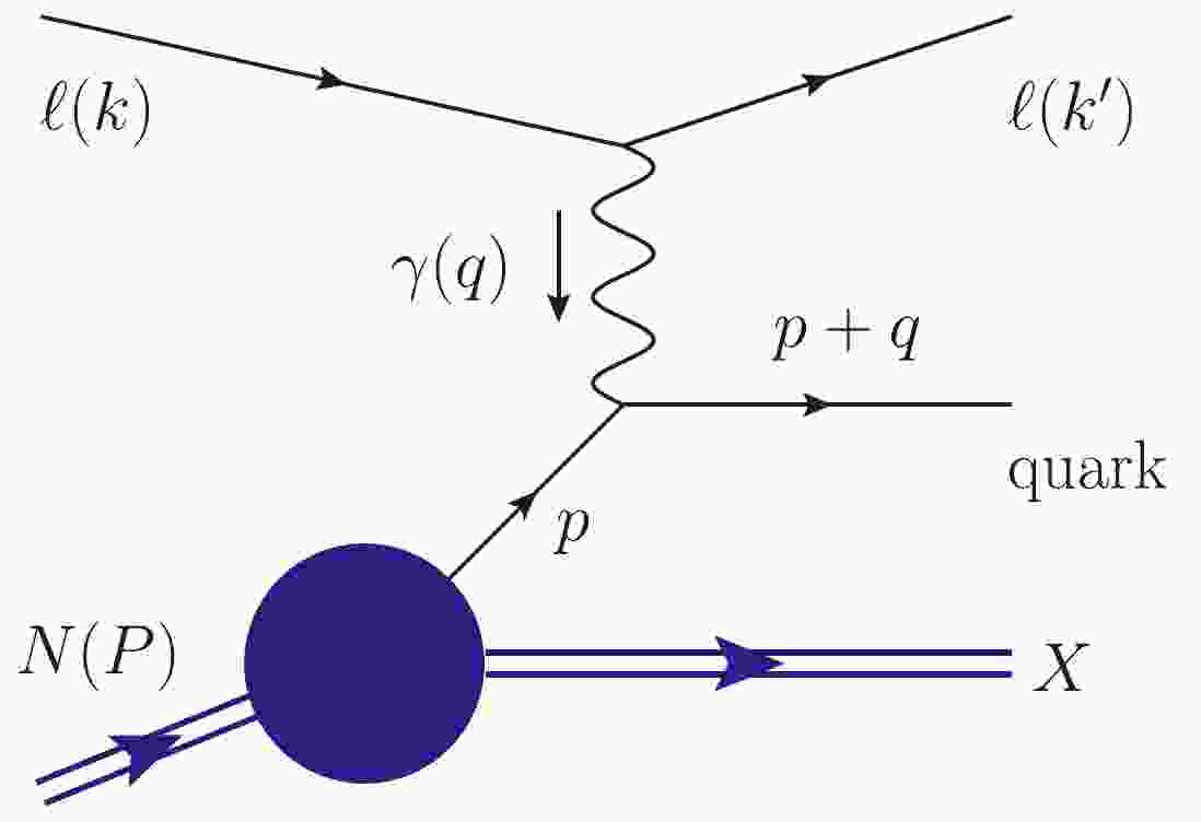
$ 0.3<x_{ \rm{B}}<0.7 $ . This phenomenon is known as the EMC effect and has been observed for a wide range of nuclei [17−21]. Here$ x_{ \rm{B}} \equiv Q^2/(2P\cdot q) $ is the Bjorken variable. Figure 1 shows the process of lepton-nucleon DIS, where a lepton with momentum k interacts with a nucleon with momentum P through the exchange of a photon; the negative squared four-momentum transfer$ Q^2\equiv -q^2 $ . Although this brought our understanding of how the quark-gluon structure of a nucleon is modified by the surrounding nucleons to a whole new level, there is still no consensus as to the underlying dynamics that drives this effect. Currently, one of the leading approaches for describing the EMC effect is that nucleons bound in nuclei are unmodified, the same as "free" nucleons most of the time, but are modified substantially when they fluctuate into SRC pairs. The connection between SRC and EMC effects has been extensively investigated in nuclear structure function measurements [22-34]. SRC pairs are conventionally defined in momentum space as a pair of nucleons with high relative momentum and low center-of-mass (c.m.) momentum, where high and low are relative to the Fermi momentum of medium and heavy nuclei. In this paper, we will emphasize the similarities between the descriptions of SRCs and Ising spins on the basis of which a new kind of map is proposed in this paper that we term the "SRC-bit map."
Figure 1. (color online) Kinematics of lepton-nucleon DIS.
The present manuscript is arranged as follows. In Sec. II, we will discuss the map between SRCs in nucleons and Ising spins. One longstanding theoretical model that is used to depict the nucleons is presented with reference to an explicit Ising model. Sec. III is devoted to simulations of nucleon states in terms of the Ising model, where our preliminary results support the proposed map between nucleons and Ising spins. Finally, we summarize our work and comment on future developments in Sec. IV.
-
In nuclei, nucleons behave approximately as independent particles in a mean field, but occasionally (
$ 20\%-25\% $ in medium or heavy nuclei) two nucleons get close enough to each other that temporarily their singular short-range interaction cannot be well described by a mean-field approximation. These are the two-nucleon short-range correlations (2N-SRC). The description of SRCs in nucleons and Ising spins in the Ising model could share the same type of observables, as with implementations of fermions within the Ising model. Ising spin$ s_i $ can take the values$ \pm 1 $ , each representing one of two spin states (spin up or down). Similarly, we define$s_{ {\rm src},i}$ to represent the state of a nucleon. For$s_{ {\rm src},i}=1$ a nucleon that belongs to an SRC pair is present at lattice site i, while for$s_{ {\rm src},i}=0$ the corresponding nucleon can be regarded as an independent particle. The simple relation between these two "spins" is$ \begin{eqnarray} s_i=2s_{ {\rm src},i}-1 \,. \end{eqnarray} $

(1) In addition to this simple relation, there are other common features between these two systems. In the Ising model, the spins are arranged in a lattice, allowing each spin to interact with its neighbors. Consider a set of lattice sites Λ. For each lattice site
$ i \in \Lambda $ there is a discrete variable$ s_i $ such that$ s_i \in \{+1,-1\} $ representing the site's spin. For any two adjacent sites$ i,j \in \Lambda $ there is an interaction J. In addition, every site$ j \in \Lambda $ is influenced by an external magnetic field h. The corresponding Hamiltonian is thus$ \begin{eqnarray} H = -\frac{J}{2}\sum_{\langle i j\rangle} s_{i} s_{j} - \mu h \sum_{j} s_{j} \,, \end{eqnarray} $

(2) where the first sum is over pairs of adjacent spins and the second term represents the universal interaction with the external magnetic field, where the magnetic moment is given by μ. The physical quantities describing nucleons can also be divided into two parts, one for nucleons belonging to SRC pairs and the other for mean-field nucleons [32]. The pedagogically sketched diagrams for the Ising model and structure of the nucleus are presented in Fig. 2. For instance, the nucleon spectral function
$ P(\mathbf{p},E) $ , which is the joint probability of finding a nucleon in a nucleus with momentum$ \mathbf{p} $ and removal energy E can be modeled as [35]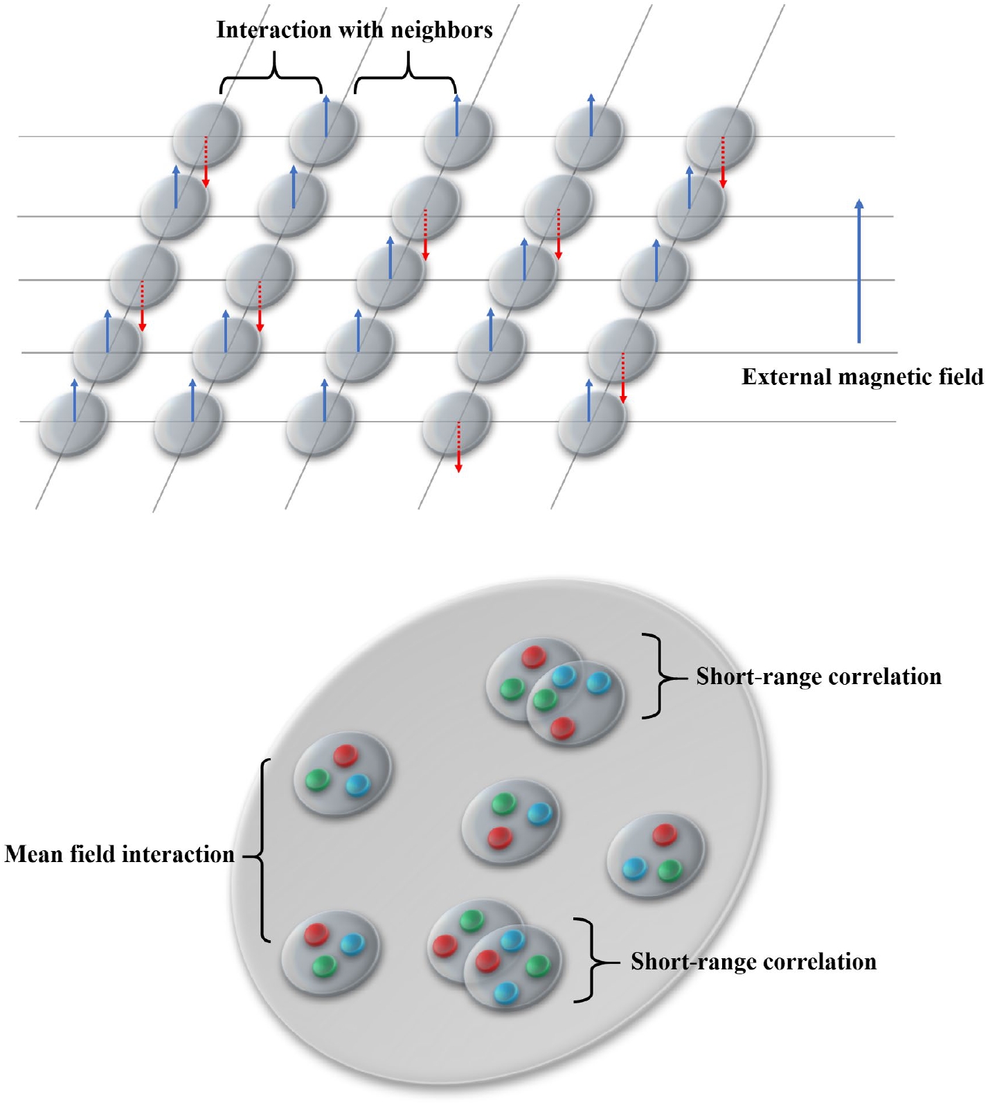
Figure 2. (color online) Schematic diagrams for the Ising model in ferromagnetism (upper) and the nuclear structure (lower), where both of the types of interactions in these diagrams can be divided into two parts. For the Ising model, they are adjacent interactions and universal external magnetic field interactions. For nuclear structure, they are SRCs and interactions with the mean field.
$ \begin{eqnarray} P(\mathbf{p}, E)= P_{1}(\mathbf{p}, E) + P_{0}(\mathbf{p}, E) \,, \end{eqnarray} $

(3) where the subscript
$ 1 $ refers to high-lying continuum states that are caused by the short-range correlations and the subscript$ 0 $ refers to values of E corresponding to low-lying intermediate excited states.Another example is the nuclear gluon distribution. We can parameterize the nuclear gluon distribution in the EMC region with the structure function [29, 36, 37]
$ \begin{eqnarray} g_{A}\left(x_{ \rm{B}}, Q^{2}\right)= 2 n_{\rm src}^{A} \delta \tilde{g}\left(x_{ \rm{B}}, Q^{2}\right) +A g_{p}\left(x_{ \rm{B}}, Q^{2}\right) \,, \end{eqnarray} $

(4) where
$n_{\rm src}^{A}$ represents the number of SRC pairs in nucleus A. Here the authors have made the approximation that all nuclear modifications originate from the nucleon-nucleon SRCs in the EMC region.$ \delta \tilde{g}\left(x_{ \rm{B}}, Q^{2}\right) $ represents the difference between the gluon distribution in the SRC pair and in the free nucleon.Inspired by the term "fermion-bit map" presented in Ref. [2], we propose an "SRC-bit map," which represents the relation between the states of each nucleon in nucleus and the state of each lattice site in the Ising model. An obvious benefit of this map is that it allows the properties of nucleons to be described in terms of classical statistical systems for Ising spins, for which many highly developed methods are available. The two-nucleon short-range correlations are defined operationally in experiments as having small center-of-mass (c.m.) momentum and large relative momentum, to which approximately
$ 20% $ nucleons belong. This means in a medium or heavy nucleus, the average$\bar{s}_{\rm src}=0\times 80\%+1\times 20\%=0.2$ , which corresponds to average Ising spin$ \bar{s}=-0.6 $ under Eq. (1).For the Hamiltonian shown in Eq. (2), the partition function is
$ \begin{eqnarray} Z=\sum_{\left\{s_i\right\}} {\rm e}^{-\beta H} \,, \end{eqnarray} $

(5) where
$\beta=(k_{\rm B} T)^{-1}$ and$ \left\{s_i\right\} $ means the sum over all possible configurations of spins. If a mean field approximation is applied, the Hamiltonian can be further simplified,$ \begin{eqnarray} H_{MF}=-\sum_{i} \mu s_i\left(h+\bar{h}\right) \,, \end{eqnarray} $

(6) here
$ \bar{h}\equiv (\mathcal{Z} J/\mu)\bar{s} $ ,$ \mathcal{Z} $ is the coordination number, and$ \bar s $ is the average Ising spin. Therefore, the partition function reads$ \begin{aligned}[b] Z_{MF} =& \prod_{i=1}^{N}\left(\sum_{s_i=\pm 1} {\rm e}^{-\beta \mu(h+\bar{h}) s_i}\right) \\ =& \left[2 \cosh \left(\frac{\mu h}{k_{\rm B} T}+\frac{\mathcal{Z} J }{k_{\rm B} T}\bar{s}\right)\right]^{N} \,. \end{aligned} $

(7) The magnetization can be written as
$ \begin{eqnarray} \left\{\begin{array}{l} M=N \mu \bar{s} \,,\\ M=-(\partial F/\partial h)=N\mu \tanh \left( \dfrac{\mu h}{k_{\rm B} T}+\dfrac{\mathcal{Z} J }{k_{\rm B} T}\bar{s} \right) \,, \end{array}\right. \end{eqnarray} $

(8) where F is the Helmholtz free energy.
$ \bar s $ can be obtained from Eq. (8)$ \begin{eqnarray} \bar{s}=\tanh \left(\frac{\mu h}{k_{\rm B} T}+\frac{\mathcal{Z} J}{k_{\rm B} T} \bar{s}\right) \,. \end{eqnarray} $

(9) Recall that
$ \bar{s}=-0.6 $ is the counterpart of$\bar{s}_{\rm src}=0.2$ . It is interesting to note the conditions under which$ \bar{s}=-0.6 $ . First, in the case of the Ising model with no external magnetic field, Eq. (9) simplifies to$ \begin{eqnarray} \bar{s}=\tanh \left(\frac{\mathcal{Z} J}{k_{\rm B} T} \bar{s}\right) \,. \end{eqnarray} $

(10) It is the coefficient
$(\mathcal{Z} J)/(k_{\rm B} T)$ that determines the solution. The upper panel of Fig. 3 shows the shapes of the r.h.s. of Eq. (10) with different coefficients. It can be seen that the desired solution$ \bar{s} = -0.6 $ can be achieved when$(\mathcal{Z} J)/(k_{\rm B} T) \approx 1.16$ . Second, in the case of the Ising model with an external magnetic field, both$(\mu h)/(k_{\rm B} T)$ and$(\mathcal{Z} J)/(k_{\rm B} T)$ contribute to the result. The lower panel of Fig. 3 presents the typical shape of the r.h.s. of Eq. (9) with solution$ \bar{s}=-0.6 $ .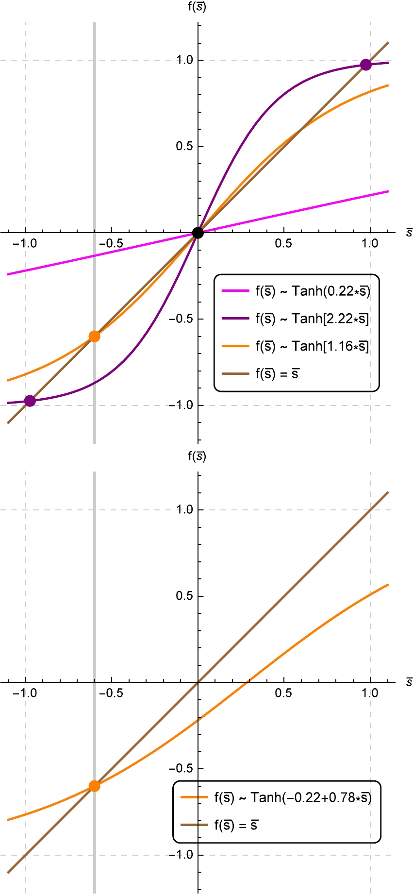
Figure 3. (color online) Upper panel shows the shapes of r.h.s. of Eq. (10) with different coefficients, where brown indicates
$ f(\bar{s})=\bar{s} $ . The desired solution (orange point) could be acquired with an appropriate choice of the coefficient$(\mathcal{Z} J)/(k_{\rm B} T)$ . The lower panel shows the typical shape of the r.h.s. of Eq. (9) with the desired solution (orange point).We would like to make a few remarks here:
1. All these discussions are independent of the particular dynamics of the systems. Sect. II therefore presents a very general map from a discrete classical statistical ensemble to the structure of the nucleus, which is formed by the strong interaction.
2. According to the simple relation in Eq. (1), there must be a phase transition in the Ising model in order to map the SRC phenomenon in the nucleus (since
$ \bar{s}=0 $ leads to$\bar{s}_{\rm src}=0.5$ , this is not the correct number as measured experimentally). In one dimension, the solution of the Ising model admits of no phase transition; thus, a higher dimensionality is needed to examine this rigorously.3. There are arguments that single-particle correlations such as momentum distributions and single-particle spectral densities are not forced to be identical between bosons and fermions in Ref. [38]. Similarly, whether the SRC-bit map would help people understand parton distribution functions such as the gluon distribution needs further investigation.
4. SRCs of more than two nucleons such as 3N-SRCs also exist in nuclei although their probability is expected to be significantly smaller than that of 2N-SRCs. Thus there would be three states of a nucleon — does not belong to SRC, or belongs to 2N-SRC or 3N-SRC. The three-state Potts model is a natural extension of the Ising model where the spin on a lattice takes one of three possible values [39]. It would be intriguing to generalize the SRC-bit map to these three states situations.
The important aspect of the Ising model is that a variety of problems can be investigated using similar kinds of modeling. Undoubtedly, with the many highly developed methods available for the Ising model, the SRC-bit map offers new insight into the study of the EMC effect in nuclear physics.
-
In the rest of this section, we will discuss a theoretical model as a potential candidate for an explicit Ising model that thus could be investigated in terms of many highly developed statistical methods. This theory was proposed by Frank, Jennings, and Miller in 1996, in which the nucleon can be regarded as a superposition of two different configurations, of which one is a "bloblike" configuration (BLC) with the normal nucleon size and the other is a "pointlike" configuration (PLC) [40, 41], Fig. 4 shows a schematic diagram of this two-component nucleon. The BLC can be thought of as an object similar to a nucleon. The PLC represents a three-quark system of small size, which dominates the high-
$ x_{ \rm{B}} $ behavior of the parton distribution function. When placed in a nucleus, the bloblike configuration feels the regular nuclear attraction and its energy decreases, while the pointlike configuration feels far less nuclear attraction. The nuclear attraction increases the energy difference between the BLCs and the PLCs, therefore reducing the PLC probability; the PLC is thus suppressed. Reducing the probability of PLCs in the nucleus reduces the quark momenta, which is in agreement with the EMC effect. One can refer to Refs. [32, 40, 41] for more details.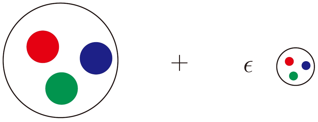
Figure 4. (color online) Two-component nucleon model: Normal-sized component plus pointlike configuration component [32].
The idea that different constituents of the nucleon have different sizes is directly related to the EMC effect [41]. The Hamiltonian is given by the matrix
$ \begin{eqnarray} H_{0}=\left[\begin{array}{cc} E_{\rm B} & V \\ V & E_{\rm P} \end{array}\right] \,, \end{eqnarray} $

(11) where
$E_{\rm P}$ and$E_{\rm B}$ are the PLC and BLC energies, respectively, and V is the hard-interaction potential that connects the two components. We choose$E_{\rm P} \gg E_{\rm B}$ and$|V| \ll E_{\rm P}-E_{\rm B}$ so that the nucleon is mainly BLC. When placed in a nucleus, the BLC component of a nucleon feels an attractive nuclear potential Hamiltonian$ H_1 $ ,$ \begin{eqnarray} H_{1}=\left[\begin{array}{ll} U & 0 \\ 0 & 0 \end{array}\right] \,. \end{eqnarray} $

(12) Therefore the complete Hamiltonian
$ H = H_0+H_1 $ is$ \begin{eqnarray} H=\left[\begin{array}{cc} E_{\rm B}-|U| & V \\ V & E_{\rm P} \end{array}\right] \end{eqnarray} $

(13) in which the attractive nature of the nuclear binding potential is emphasized. The inclusion of U increases the energy difference between the BLC and the PLC components, which decreases the PLC probability. Within this model the medium-modified nucleon contains a component that is an excited state of a free nucleon. The amount of modification that gives a deviation of the EMC ratio from unity is controlled by the potential U. The eigenstates of H are labeled
$ | N \rangle_M $ and$ | N^* \rangle_M $ , where the subscript M means medium-modified; they are$ \begin{aligned}[b] | N \rangle_{M} = |B\rangle+\epsilon_{M}|P\rangle \,, \quad | N^{*} \rangle_{M} = -\epsilon_{M}|B\rangle+|P\rangle \,, \end{aligned} $

(14) where
$\epsilon_{M} = V/(E_{\rm B}-|U|-E_{\rm P})$ ,$ |B\rangle $ stands for the BLC state, and$ |P\rangle $ stands for the PLC state. One can also write down the eigenstates of$ H_0 $ ,$ \begin{aligned}[b] |N\rangle = |B\rangle+\epsilon|P\rangle \,, \quad |N^{*}\rangle = -\epsilon|B\rangle+|P\rangle \,, \end{aligned} $

(15) with
$\epsilon = V/(E_{\rm B}-E_{\rm P})$ . Therefore, the medium-modified nucleon$ |N\rangle_{M} $ can be expressed in terms of the unmodified eigenstates$ |N\rangle $ and$ |N^*\rangle $ as$ \begin{eqnarray} |N\rangle_{M} \approx |N\rangle+\left(\epsilon_{M}-\epsilon\right)|N^{*}\rangle \,. \end{eqnarray} $

(16) It is the second term whose functionality resembles the SRC pair described above that dominates the high-
$ x_{ \rm{B}} $ behavior of structure function, i.e., the EMC effect measured in DIS experiments. By adjusting the amount of the excited state$ |N^{*}\rangle $ contained in nucleon$ |N\rangle_{M} $ , the deviation of the EMC ratio from unity can be predicted [41, 42]. In this theory, the degree of deviation is controlled by U, V and$ E_{\rm P}-E_{\rm B} $ . One can use$ s_{ \rm{src}}=1 $ to represent the excited state$ |N^{*}\rangle $ and$ s_{ \rm{src}}=0 $ for the ground state$ |N\rangle $ . According to the simple relation in Eq. (1), their correspondences are with lattice sites with spin$ s=1 $ and$ s=-1 $ , respectively. For an Ising model in a certain dimension, the variables that determine the final magnetization state are the temperature T, coupling J, and external magnetic field h.One can envision the following situation: Before being bound in a nucleus, the nucleons can be regarded as collections of "free particles" whose components are
$ |N\rangle = |B\rangle+\epsilon|P\rangle $ . It is the potential V that connects the two components; the amount of PLC decreases with the increase of$ V^{-1} $ , in which case most would be BLC. This is very similar to the Ising model in ferromagnetism without an external magnetic field, where the states of the lattice tends to be the same with the increase of coupling J. The energy difference$\Delta E=E_{\rm P}-E_{\rm B}$ is also an important factor; the numbers of BLC and PLC would be approximately equal when$ \Delta E^{-1} \to \infty $ , analogous to the case of no phase transition when$ T\to\infty $ which is provided as an acceptance criterion for different spin states in the Ising model. For$ \Delta E^{-1} \to 0 $ , the huge energy difference indicates there are few PLCs in the nucleon, corresponding to no SRC pair. Similarly, when$ T\to 0 $ , nearly all of the spin states are the same in the Ising model.Now suppose the nucleons are bound in a nucleus. They would feel an attractive nuclear potential U, which further decreases the PLC probability according to Eq. (14). A similar situation occurs in paramagnetics when we add a downward external magnetic field h, which converts more spin states of lattice sites to
$ -1 $ . From this point of view, the general properties of the variables used to describe the models of nucleons and Ising spins are the same. -
We will explore the issue of simulating the nucleon states in the nucleus in terms of mature methods available for a two-dimensional square lattice Ising model in greater detail. In general, a Monte Carlo simulation processes a subset of configurations in the configuration space of a given system according to a predefined probability distribution. Here we set the states of all lattice sites to
$ -1 $ as our predefined distribution. Eq. (1) allows us to relate the$ s=-1 $ to$ s_{ \rm{src}}=0 $ of the nucleon state, which corresponds to the situation where all the nucleons do not belong to SRCs.The Metropolis algorithm will be utilized to perform the importance sampling of the configuration space [43]. In this method, a Markov chain of configurations is generated in which each configuration
$ C_{\ell+1} $ is obtained from the previous one$ C_{\ell} $ with a suitably chosen transition probability$ \omega_{(\ell \to \ell+1)} $ determined by the Metropolis function$ \begin{eqnarray} \omega_{(\ell \to \ell+1)}=\min \left[1, \exp \left(-\frac{\Delta E}{k_{\rm B} T}\right)\right] \,, \end{eqnarray} $

(17) i.e.,
$ \begin{eqnarray} \left\{\begin{aligned} & \omega_{(\ell \to \ell+1)} = \exp \left(-\frac{\Delta E}{k_{\rm B} T}\right)\,, & ~~ \text { if }~~ \Delta E>0 \,,\\ & \omega_{(\ell \to \ell+1)} = 1\,, & ~~ \text { if }~~ \Delta E<0 \,. \nonumber \end{aligned}\right.\\ \end{eqnarray} $

where
$ \Delta E = E(C_{\ell+1}) - E(C_{\ell}) $ . The process$ C_{\ell} \to C_{\ell+1} $ constitutes one Monte Carlo step (MCS), which may be taken as our unit of computational "time." We will take the time to$ 1\times 10^6 $ in our simulation. -
The Hamiltonian of the Ising model has already been shown in Eq. (2). We will modify this Hamiltonian to make it more suitable for describing nucleons. The states of nucleons are simulated on a
$ 400\times400 $ lattice, and these$ 1.6\times 10^5 $ lattice sites are grouped into$ 8\times 10^4 $ pairs, taking into account that SRCs always appear in pairs. The spin of any pair of sites is either$ +1 $ or$ -1 $ , where the value of coupling J depends on the magnetization state of the system.We divide the first term in Eq. (2), which describes the interaction between adjacent spins, into two parts, one responsible for the adjacent interaction between a pair of
$ +1 $ states, the other accounting for the interaction between a pair of$ -1 $ states. The modified Hamiltonian of the Ising model is$ \begin{aligned}[b] & H =-2C \, J_{ \rm{up}}\sum_{\langle i \rangle} s_{i} + 2C \, J_{ \rm{down}}\sum_{\langle j \rangle} s_{j} - \mu h \sum_{\langle j' \rangle} s_{j'} \,, \\ & \text { for~ any }~ s_{i}=+1 ~ \text{and}~ s_{j,j'}=-1 \,. \end{aligned} $

(18) The first sum runs over all pairs of nucleons with
$ s=+1 $ , and the second sum is over all pairs with$ s=-1 $ . The factor$ 2 $ is introduced to remind us that there are two lattice sites with same spin in one pair; the energy dimension of coefficient C is$ E^1 $ , which serves to characterize the relative interaction strength compared to the external magnetic field. The third sum depicts the universal interaction with external magnetic field, where we take h to have a negative value and whose functionality only acts on the$ -1 $ states, reducing the energy of this system. This is consistent with the function of U in the theoretical model introduced at the previous section in Eq. (12). In this modified Ising model, the$ J_{ \rm{up}} $ and$ J_{ \rm{down}} $ terms account for the short-range interaction and the magnetic field μ term accounts for the long-range interaction. It is under their combined effects that the system reaches its equilibrium state. It is worth noting that the relative values of$ J_{ \rm{up}} $ ,$ J_{ \rm{down}} $ , and h characterize the relation between short-range and long-range interactions on nucleons, which is an important research object since this relation decides the magnitude of the EMC effect.The form of the modified Hamiltonian is not unique. We constructed Eq. (18) specifically for our purpose of describing the states of nucleons statistically, although this step will introduce model dependence. The construction of the modified Ising model is not determined, leading to the results being dependent on the form of the model and selection of its parameters.
One important feature of the Metropolis algorithm shown in Eq. (17) is that it allows MCS, which increases the energy, albeit with a low probability if the energy is increased by a large amount. The variation of energy in every MCS is influenced by the couplings
$ J_{ \rm{up}} $ and$ J_{ \rm{down}} $ , which are expressed in terms of the average Ising spin in this modified Ising model,$ \begin{eqnarray} \left\{\begin{aligned} & J_{ \rm{up}} = -\frac{1}{L^2} \sum_{\mu} s_\mu = -\bar s \,,\\ & J_{ \rm{down}} = 1+\frac{1}{L^2} \sum_{\mu} s_\mu = 1+\bar s \,. \end{aligned}\right. \end{eqnarray} $

(19) Before simulation, we also need to specify the initial configuration; here it is all spins pointing down (i.e.,
$ s_i=-1 $ for all i) at$ t=0 $ . This configuration corresponds to a bunch of "free" nucleons without SRC pairs. Then we add an external magnetic field and allow this system to evolve until it reaches the equilibrium distribution. The simulation results will be shown in next section. -
Here we present the final simulation results for the modified Ising model used to mimic the nucleons bound in a medium or heavy nucleus. Figure 5 presents the evolution of the system from initial state (
$ s_i = -1 $ for all i) to equilibrium state. After the completion of$ 1\times10^6 $ MCS, the ratio of the two components (nucleon belonging to an SRC or not) is maintained at$ 1/4 $ at$ T=2.5 $ , which is consistent with experimental data. In this simulation, we take the coefficient$ C=2 $ and the external field$ h=-4 $ . Figure 6 shows the stability of this simulation; after$ 1\times 10^5 $ MCS,$ \bar s $ remains at about$ -0.6 $ .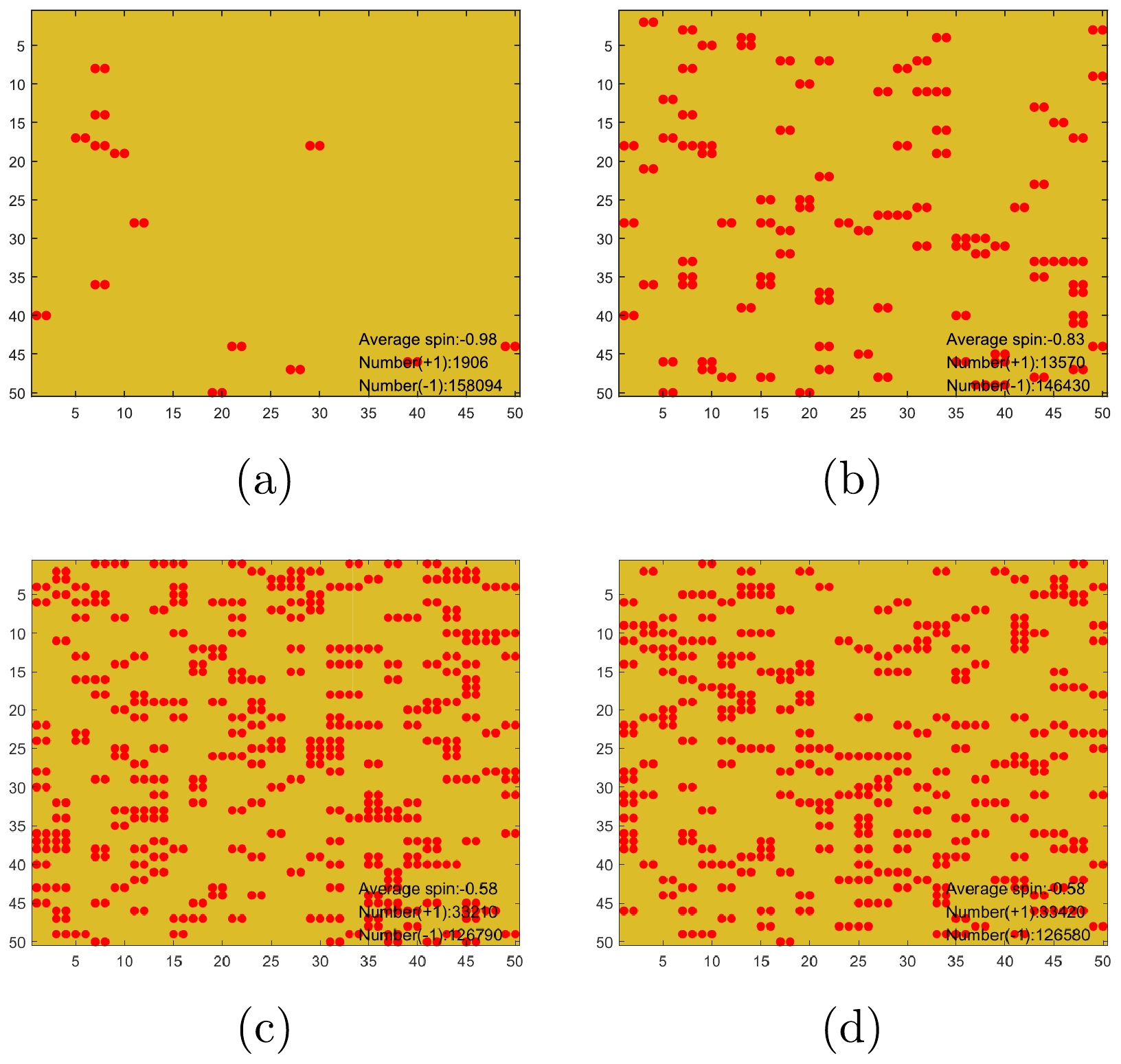
Figure 5. (color online) Simulation of bound nucleons in terms of a two-dimensional lattice of size
$ 400\times 400 $ sites; here we only show a small part of the simulation micrograph ($ 50\times 50 $ ) for a better view. Every pair of red balls indicates a pair of SRCs; the other lattice sites, in yellow, represent nucleons that are nearly free. Micrograph (a) is taken after the completion of$ 1\times 10^3 $ MCSs, where the memory of the initial configuration has not been lost. Micrograph (b) is taken after$ 1\times 10^4 $ MCS, where the variation of the system tends to be gentle. Micrographs (c) and (d) are taken after$ 5\times 10^5 $ and$ 1\times 10^6 $ MCSs, respectively; these two diagrams indicate that the system has reached an equilibrium state. When$ T=2.5 $ , the ratio of the two components is maintained at$ 1/4 $ .
Figure 6. (color online) Average spin vs time, clearly showing that the average spin of this system stabilizes at about
$ \bar s=-0.6 $ after$ 1\times 10^5 $ MCS, which is consistent with the micrographs in Fig. 3.The average spin
$ \bar s $ vs temperature T curve is plotted in Fig. 7. As is evident from this figure, the system tends to be more disordered (i.e.,$ \bar s \to 0 $ ) as the temperature increases, whose corresponding situation in the nucleus has been described in the last section as$ \Delta E^{-1} \to \infty $ . In many nuclear theories, the temperature is related to the energy difference between different states of nucleons; thus, we can investigate the distinction between nucleons in the SRC state and normal state by scrutinizing the temperature dependence in the Ising model. Figure 8 presents the influence of the external magnetic field h on$ \bar s $ . When it reaches the equilibrium state, the system is more orderly (i.e.,$ \bar s \to -1 $ ) as$ |h| $ increases.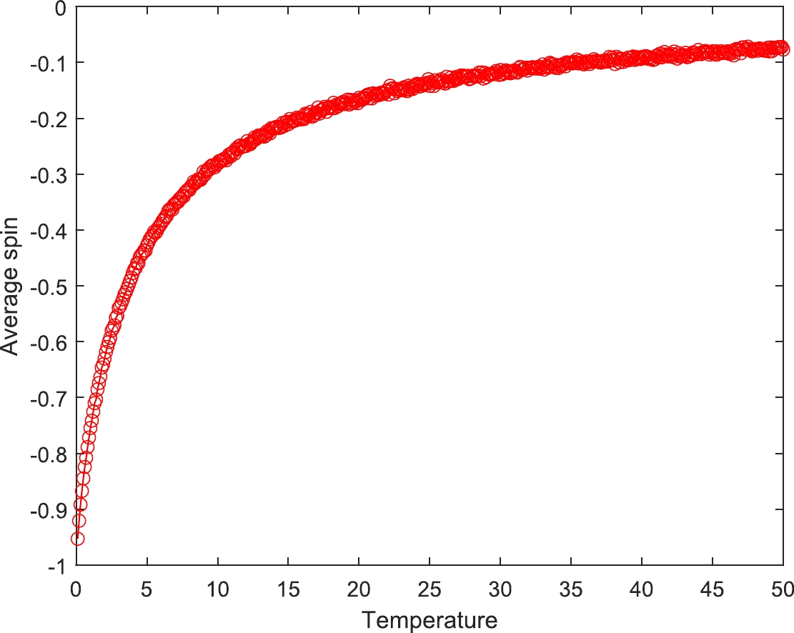
Figure 7. (color online) Average spin vs temperature, where the values are taken after
$ 1\times 10^6 $ MCS, where C and h are fixed at$ 2 $ and$ -4 $ , respectively.$ |\bar s| $ decreases with increasing temperature.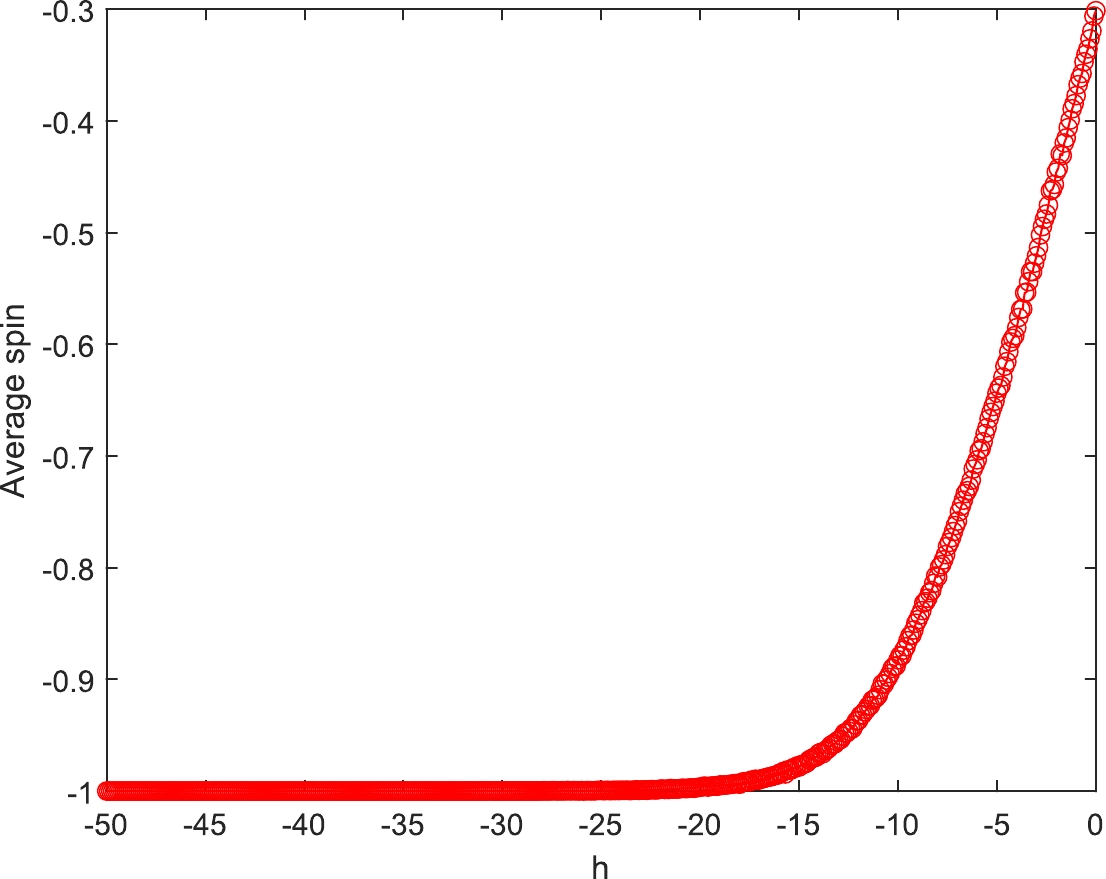
Figure 8. (color online) Average spin vs external magnetic field, where the values are taken after
$ 1\times 10^6 $ MCS; here,$ C=2 $ and$ h=-4 $ .$ |\bar s| $ increases with increasing$ |h| $ .The results shown in this section have qualitatively confirmed the validity of utilizing the Ising model to describe the states of nucleons bound in a nucleus. This encouraging result indicates the possibility of investigating nucleons in terms of many well established techniques in thermodynamic statistics, which in some sense assumes that the fundamental mechanism of the real world is intrinsically probabilistic. Classical statistics and quantum mechanics are two sides of the same coin, rather than mutually exclusive concepts. In many cases, the typical quantum mechanical features emerge if we concentrate on the statistical description of the system for a particle. This opens the potential for cross-fertilization between the two formalisms, since they both can describe the same physical reality.
On the other hand, Quantum Chromodynamics (QCD) is our fundamental theory to describe the structure of the nucleon. As a nonperturbative approach based on first principles, lattice QCD (LQCD) can in principle be applied to resolve this issue. In fact, there is a pioneering work in which the fraction of the longitudinal momentum of
$ ^3 \rm{He} $ that is carried by the isovector combination of u and d quarks is determined using lattice QCD for the first time [33]. This work shows potential for revealing the QCD origins of the EMC effect. The authors intend to expand the range of nuclei and provide a complete flavor decomposition in the near future. It is worth noting that Ref. [33] did not observe the EMC effect in their lattice simulations, which in some sense is to be expected due to the limited computing resources (e.g., the unphysical π mass,$ m_\pi \sim 800\, \rm{MeV} $ ) and the choice of a light nucleus ($ ^3 \rm{He} $ ). Nevertheless, we believe this marks significant progress despite the great cost in computing resources and need for new efficient algorithms. This situation thus raises the question whether we can use a simple statistical model to capture the main features of nucleon structure; this paper reports our first attempt on this issue.Here, we note that the simulation in this manuscript is rather rough and the results are fairly sensitive to the model construction. The value of average spin will stabilize elsewhere than
$ -0.6 $ if the parameters in Eq. (18) are changed (as shown in Fig. 6 and Fig. 7). Therefore, to realize the power of the Ising model, systematic studies on parameter selection are urgently needed. Besides, the estimation of$20\%$ of the nucleons belonging to SRCs in medium or heavy nuclei needs to be explored in more detail; this Ising-model-based simulation should be able to describe a series of nuclei explicitly and reproduce the linear relation between the magnitude of the EMC effect and SRC scale factor [26].In short, we construct a modified Ising model in Eq. (18) that is implemented through a Monte Carlo calculation to describe the nucleons bound in nucleus. As suggested by the simple map in Eq. (1), the average spin of this model should stabilize at about
$ \bar s=-0.6 $ when it reaches the equilibrium state, as mentioned in Sec. II. Our results here yield positive insights into applying the Ising model to this issue. -
Based on the fact that the SRCs in nucleons and Ising spins in the Ising model could share the same type of observables, a new SRC-bit map is proposed in this work. This map is a powerful tool connecting the state of each nucleon with the state of each lattice site. We have considered a nuclear theory as a correspondence to an explicit Ising model and implemented a simulation of the nucleon states in terms of the Ising model; our preliminary results support the proposed map between nucleons and Ising spins.
The investigation of nucleons with the SRC-bit map is evidently in the nascent stage, but with advancements in computational sources and efficient algorithms, the prospect of its applications in research areas related to nuclear structure appears bright. More rigorous investigations of related issues are urgently called for. Besides conceptual advances, the treatment of classical statistics and quantum particles in a common formalism could lead to unexpected cross-fertilization on both sides.
-
We thank Prof. Wei Wang, Dr. Shuai Zhao, and Dr. Jian-Ping Dai for valuable discussions.
Nucleons as modified Ising models
- Received Date: 2023-04-06
- Available Online: 2023-09-15
Abstract: In this paper, we propose a map that connects nucleons bound in nuclei and Ising spins in the Ising model. This proposal is based on the fact that the description of states of nucleons and Ising spins could share the same type of observables. We present a nuclear model corresponding to an explicit modified Ising model and qualitatively confirm the correctness of this map with a simulation on a two-dimensional square lattice. This map can help us understand the profound connections between different physical systems.


 DownLoad: