


 Abstract
 HTML
HTML Reference
 Related
 PDF
PDF


-
In the past years, several excited bottom baryon states
$ \Lambda_b $ [1−3] and excited strange-bottom baryon states$ \Xi_b $ [4−10] have been observed. In 2012, the LHCb collaboration observed two narrow states,$ \Lambda_b(5912)^0 $ and$ \Lambda_b(5920)^0 $ , in the$ \Lambda_b^0 \pi^+\pi^- $ invariant mass spectrum [3]. The masses were measured to be$ \begin{aligned}[b] & M_{\Lambda_b(5912)} = 5911.97\pm0.12 \pm0.02 \pm0.66 \rm{ MeV}\,, \\ & M_{\Lambda_b(5920)} = 5919.77 \pm0.08 \pm0.02 \pm0.66 \rm{ MeV}\,. \end{aligned} $

(1) In 2021, the CMS collaboration discovered
$ \Xi_b(6100)^- $ in the$ \Xi_b^- \pi^+\pi^- $ invariant mass spectrum with spin-parity$J^P={3}/{2}^-$ [9]; the measured mass was$ \begin{align} &M_{\Xi_b(6100)} = 6100.3\pm0.2 \pm0.1 \pm0.6 \rm{ MeV}\, . \end{align} $

(2) Sometime ago, the LHCb collaboration confirmed
$ \Xi_b(6100)^- $ in decay mode$ \Xi_b^{*0}\pi^- $ , and observed bottom baryon states$ \Xi_b(6087)^0 $ and$ \Xi_b(6095)^0 $ in decay modes$ \Xi_b^{\prime-} \pi^+ $ and$ \Xi_b^{*-} \pi^+ $ , respectively [11, 12]; the masses and widths were determined to be$ \begin{aligned}[b] & M_{\Xi_b(6100)} = 6099.74\pm0.11\pm0.02\pm0.6 \rm{ MeV}\,,\,\,\\&\Gamma_{\Xi_b(6100)} = 0.94\pm0.30\pm0.08 \rm{ MeV} \, , \\ & M_{\Xi_b(6087)} = 6087.24\pm0.20 \pm0.06 \pm0.5 \rm{ MeV}\,,\\&\Gamma_{\Xi_b(6087)} = 2.43 \pm0.51 \pm0.10 \rm{ MeV} \, , \\ & M_{\Xi_b(6095)} = 6095.26 \pm0.15 \pm0.03 \pm0.5 \rm{ MeV}\,,\\&\Gamma_{\Xi_b(6095)} = 0.50 \pm0.33 \pm0.11\rm{ MeV} \, . \end{aligned} $

(3) We can tentatively assign
$ \Xi_b(6095)^0 $ and$ \Xi_b(6100)^- $ to be the isospin doublet by considering the mass difference and quark constituents.Experimental discoveries of those single bottom baryon states have increased the interest in theoretical research. It is necessary to identify the quantum numbers of those states and explore their internal structures. The bottom baryon states have been investigated using many theoretical approaches, including the elementary emission model and
$ {}^3P_0 $ model (quark pair creation model) [13] ([14]), chiral quark model [15, 16], constituent quark model [17−19], QCD-motivated relativistic quark model [20], light-cone QCD sum rule [21], QCD sum rules [22−31], and lattice QCD [32]. In particular,$ \Lambda_b(5912) $ and$ \Lambda_b(5920) $ have been investigated by the flux tube model [33], QCD sum rules combined with the heavy quark effective theory [34], effective hadronic model with respect to the chiral and heavy-quark spin-flavor symmetries [35], relativized quark model [36], etc. These studies showed that$ \Lambda_b(5912) $ and$ \Lambda_b(5920) $ can be accommodated in the 1P states with$J^P={1}/{2}^-$ and${3}/{2}^-$ , respectively. Additionally,$ \Xi_b(6100) $ can be taken as a good candidate for the 1P bottom state with$J^P={3}/{2}^-$ by the$ {}^3P_0 $ model [37], QCD sum rules combined with the heavy quark effective theory [38], relativized quark model [39], etc.In previous studies of ours, we used the full QCD sum rules to systematically investigate the heavy baryon states. We calculated the masses of the S-wave, P-wave and D-wave charmed baryon candidates
$ \Omega_c(3000) $ ,$ \Omega_c(3050) $ ,$ \Omega_c(3066) $ ,$ \Omega_c(3090) $ ,$ \Omega_c(3119) $ [40, 41],$ \Omega_c(3327) $ [42],$ \Lambda_c(2625) $ [43],$ \Xi_c(2815) $ [43],$ \Lambda_c(2860) $ ,$ \Lambda_c(2880) $ ,$ \Xi_c(3055) $ , and$ \Xi_c(3080) $ [44], and acquired satisfactory results consistent with the experimental data that will set guidelines for future experimental measurements. On the bottom sector, our calculations also led to satisfactory assignments for P-wave candidates$ \Omega_b(6316) $ ,$ \Omega_b(6330) $ ,$ \Omega_b(6340) $ , and$ \Omega_b(6350) $ [30] and D-wave candidates$ \Lambda_b(6146) $ ,$ \Lambda_b(6152) $ ,$ \Xi_b(6327) $ , and$ \Xi_b(6333) $ [29].In the constituent quark models, the
$ \Xi_b $ states have three valence quarks$ q\,(u,d) $ , s and b. Introducing the relative P-wave between q and s in the diquarks, we obtained the Λ-type$ \Xi_b $ baryon states with spin-parity$J^P={1}/{2}^-$ ,${3}/{2}^-$ . We can choose either a partial derivative$ \partial_\mu $ or covariant derivative$D_\mu=\partial_\mu-{\rm i} g_sG_\mu$ to embody the net effects of the relative P-wave. It is interesting to choose both partial$ \partial_\mu $ and covariant$ D_\mu $ derivatives in constructing the P-wave states, and examine the different outcomes, similar to previous studies of ours on the D-wave charmed baryon states [42]. In this study, we comprehensively explore the P-wave Λ-type bottom baryon states using the QCD sum rules, and examine the sub-structures of new bottom baryon states$ \Lambda_b(5912) $ ,$ \Lambda_b(5920) $ ,$ \Xi_b(6087) $ ,$ \Xi_b(6095) $ , and$ \Xi_b(6100) $ to diagnose their nature, because their properties are not completely understood yet.The paper is structured as follows: the P-wave bottom baryon states are studied via the QCD sum rules in Section II; numerical results and discussion are provided in Section III; in Section IV, relevant conclusions are drawn.
-
First, let us express the two-point correlation functions
$ \Pi(p) $ and$ \Pi_{\mu\nu}(p) $ ,$ \begin{aligned}[b] \Pi(p)=&{\rm i}\int {\rm d}^4x {\rm e}^{{\rm i}p \cdot x} \langle0|T\left\{J/\eta(x) \bar{ J}/\bar{\eta}(0)\right \}|0\rangle \, , \\ \Pi_{\mu\nu}(p)=&{\rm i}\int {\rm d}^4x {\rm e}^{{\rm i}p \cdot x} \langle0|T\left\{J/\eta_\mu(x)\bar{J}/\bar{\eta}_\nu(0)\right \}|0\rangle \, , \end{aligned} $

(4) where
$ \begin{aligned}[b] J(x)=&J^{\Lambda_b}(x)\, , \,\, J^{\Xi_b}(x)\, , \\ \eta(x)=& \eta^{\Lambda_b}(x)\, , \,\,\eta^{\Xi_b}(x)\, , \\ J_\mu(x)=&J_{1,\mu}^{\Lambda_b}(x)\, ,\,\,J_{2,\mu}^{\Lambda_b}(x)\, ,\,\, J_{1,\mu}^{\Xi_b}(x)\, ,\,\,J_{2,\mu}^{\Xi_b}(x)\, , \\ \eta_\mu(x)=& \eta_{1,\mu}^{\Lambda_b}(x)\, , \,\, \eta_{2,\mu}^{\Lambda_b}(x)\, ,\, \, \eta_{1,\mu}^{\Xi_b}(x)\, ,\,\,\eta_{2,\mu}^{\Xi_b}(x)\, , \end{aligned} $

(5) $ \begin{aligned}[b]\\[-10pt] J^{\Lambda_b}(x) =&\varepsilon^{ijk} \left[ \partial^\mu u^T_i(x) C\gamma^\nu d_j(x)- u^T_i(x) C\gamma^\nu \partial^{\mu}d_j(x)\right]\sigma_{\mu\nu}\,b_k(x) \, , \\ J_{1,\mu}^{\Lambda_b}(x)=&\varepsilon^{ijk} \left[ \partial^\alpha u^T_i(x) C\gamma^\beta d_j(x)-u^T_i(x) C\gamma^\beta \partial^{\alpha}d_j(x)\right]\left(\widetilde{g}_{\mu\alpha}\gamma_\beta-\widetilde{g}_{\mu\beta}\gamma_\alpha \right){\rm i}\gamma_5 b_k(x) \, , \\ J_{2,\mu}^{\Lambda_b}(x)=&\varepsilon^{ijk} \left[ \partial^\alpha u^T_i(x) C\gamma^\beta d_j(x)- u^T_i(x) C\gamma^\beta \partial^{\alpha}d_j(x)\right] \left(g_{\mu\alpha}\gamma_\beta+g_{\mu\beta}\gamma_\alpha-\frac{1}{2}g_{\alpha\beta}\gamma_\mu \right){\rm i}\gamma_5 b_k(x)\, , \\ \end{aligned} $ 
(6) $ \begin{aligned}[b] \eta^{\Lambda_b}(x) =&\varepsilon^{ijk} \left[ D^\mu u^T_i(x) C\gamma^\nu d_j(x)- u_i(x) C\gamma^\nu D^{\mu}d_j(x)\right]\sigma_{\mu\nu}\,b_k(x) \, , \\ \eta_{1,\mu}^{\Lambda_b}(x)=&\varepsilon^{ijk} \left[ D^\alpha u^T_i(x) C\gamma^\beta d_j(x)-u^T_i(x) C\gamma^\beta D^{\alpha}d_j(x)\right]\left(\widetilde{g}_{\mu\alpha}\gamma_\beta-\widetilde{g}_{\mu\beta}\gamma_\alpha \right){\rm i}\gamma_5 b_k(x) \, , \\ \eta_{2,\mu}^{\Lambda_b}(x) =&\varepsilon^{ijk} \left[ D^\alpha u^T_i(x) C\gamma^\beta d_j(x)- u^T_i(x) C\gamma^\beta D^{\alpha}d_j(x)\right] \left(g_{\mu\alpha}\gamma_\beta+g_{\mu\beta}\gamma_\alpha-\frac{1}{2}g_{\alpha\beta}\gamma_\mu \right){\rm i}\gamma_5 b_k(x) \, , \\ \end{aligned} $

(7) $ \begin{aligned}[b] J^{\Xi_b}(x) =&\varepsilon^{ijk} \left[ \partial^\mu q^T_i(x) C\gamma^\nu s_j(x)- q^T_i(x) C\gamma^\nu \partial^{\mu}s_j(x)\right]\sigma_{\mu\nu}\,b_k(x) \, , \\ J_{1,\mu}^{\Xi_b}(x)=&\varepsilon^{ijk} \left[ \partial^\alpha q^T_i(x) C\gamma^\beta s_j(x)-q^T_i(x) C\gamma^\beta \partial^{\alpha}s_j(x)\right]\left(\widetilde{g}_{\mu\alpha}\gamma_\beta-\widetilde{g}_{\mu\beta}\gamma_\alpha \right){\rm i}\gamma_5 b_k(x) \, , \end{aligned} $

$ \begin{aligned}[b] J_{2,\mu}^{\Xi_b}(x)=&\varepsilon^{ijk} \left[ \partial^\alpha q^T_i(x) C\gamma^\beta s_j(x)- q^T_i(x) C\gamma^\beta \partial^{\alpha}s_j(x)\right] \left(g_{\mu\alpha}\gamma_\beta+g_{\mu\beta}\gamma_\alpha-\frac{1}{2}g_{\alpha\beta}\gamma_\mu \right){\rm i}\gamma_5 b_k(x)\, , \\ \end{aligned} $

(8) $ \begin{aligned}[b] \eta^{\Xi_b}(x) =&\varepsilon^{ijk} \left[ D^\mu q^T_i(x) C\gamma^\nu s_j(x)- q^T_i(x) C\gamma^\nu D^{\mu}s_j(x)\right]\sigma_{\mu\nu}\,b_k(x) \, , \\ \eta_{1,\mu}^{\Xi_b}(x)=&\varepsilon^{ijk} \left[ D^\alpha q^T_i(x) C\gamma^\beta s_j(x)-q^T_i(x) C\gamma^\beta D^{\alpha}s_j(x)\right]\left(\widetilde{g}_{\mu\alpha}\gamma_\beta-\widetilde{g}_{\mu\beta}\gamma_\alpha \right){\rm i}\gamma_5 b_k(x) \, , \\ \eta_{2,\mu}^{\Xi_b}(x)=&\varepsilon^{ijk} \left[D^\alpha q^T_i(x) C\gamma^\beta s_j(x)- q^T_i(x) C\gamma^\beta D^{\alpha}s_j(x)\right] \left(g_{\mu\alpha}\gamma_\beta+g_{\mu\beta}\gamma_\alpha-\frac{1}{2}g_{\alpha\beta}\gamma_\mu \right){\rm i}\gamma_5 b_k(x)\, , \end{aligned} $

(9) $ q=u $ or d, the i, j, k are color indexes, C is the charge conjugation matrix, and$\widetilde{g}_{\mu\alpha}=g_{\mu\alpha}- {1}/{4}\gamma_\mu\gamma_\alpha$ is the tensor structure. We choose both partial$ \partial_\mu $ and covariant$ D_\mu $ derivatives to construct the currents;$ J/\eta(x) $ and$ J/\eta_\mu(x) $ interpolate the P-wave baryon states with spin-parity$J^P={{1}/{2}}^-$ and${{3}/{2}}^-$ , respectively. The currents with covariant derivatives are gauge covariant/invariant; however, this disfavors the interpretation of the covariant derivatives as angular momenta in the non-relativistic limit, i.e.,$ D \to \vec{p}+g_s\vec{G} $ . By contrast, the currents with partial derivatives$ \partial_\mu $ are not gauge covariant; however, this does favor the interpretation of the partial derivatives as angular momentum in the non-relativistic limit, i.e.,$ \partial \to \vec{p} $ . In the quantum field theory, gauge invariant currents are constructed with the same quantum numbers as the hadrons to interpolate them, and it suffices. In this sense, the gauge invariant currents are physical and preferred.Diquarks
$\varepsilon^{ijk} q^T_i(x) C\gamma_\alpha \stackrel{\leftrightarrow}{\partial}_\beta q^\prime_j(x)$ and$\varepsilon^{ijk} q^T_i(x) \times C\gamma_\alpha \stackrel{\leftrightarrow}{D}_\beta q^\prime_j(x)$ have two Lorentz indexes α and β, where$ q\neq q^\prime $ ,$ \stackrel{\leftrightarrow}{\partial}_\beta=\stackrel{\rightarrow }{\partial}_\beta -\stackrel{\leftarrow}{\partial}_\beta $ and$ \stackrel{\leftrightarrow}{D}_\beta=\stackrel{\rightarrow }{D}_\beta-\stackrel{\leftarrow}{D}_\beta $ . Structures$ C\gamma_\alpha \stackrel{\leftrightarrow}{\partial}_\beta $ and$ C\gamma_\alpha \stackrel{\leftrightarrow}{D}_\beta $ are antisymmetric. Therefore, currents$ J/\eta(x) $ and$ J/\eta_\mu(x) $ are referred to as Λ-type currents. Dirac matrices$ \widetilde{g}_{\mu\alpha}\gamma_\beta-\widetilde{g}_{\mu\beta}\gamma_\alpha $ and$g_{\mu\alpha}\gamma_\beta + g_{\mu\beta}\gamma_\alpha-\dfrac{1}{2}g_{\alpha\beta}\gamma_\mu$ are anti-symmetric and symmetric, respectively, when interchanging indexes α and β, which are constructed with the corresponding indexes in the diquarks. Therefore, the diquarks in currents$ J/\eta_{1,\mu}(x) $ and$ J/\eta_{2,\mu}(x) $ have spins 1 and 2, respectively.Currents
$ J/\eta(0) $ and$ J/\eta_\mu(0) $ couple potentially to$J^P={{1}/{2}}^\mp$ and${{1}/{2}}^\pm$ ,${{3}/{2}}^\mp$ and bottom baryon states$B_{{1}/{2}}^\mp$ and$B_{{1}/{2}}^\pm$ ,$B_{{3}/{2}}^\mp$ , respectively,$ \begin{aligned}[b] \langle 0| J/\eta (0)|B_{\frac{1}{2}}^-(p)\rangle =&\lambda^-_{\frac{1}{2}} U^-(p,s) \, , \\ \langle 0| J/\eta (0)|B_{\frac{1}{2}}^+(p)\rangle =&\lambda^+_{\frac{1}{2}}{\rm i}\gamma_5 U^+(p,s) \, , \\ \langle 0| J/\eta_{\mu} (0)|B_{\frac{3}{2}}^-(p)\rangle =&\lambda^-_{\frac{3}{2}} U^-_\mu(p,s) \, , \\ \langle 0| J/\eta_{\mu} (0)|B_{\frac{3}{2}}^+(p)\rangle =&\lambda^+_{\frac{3}{2}}{\rm i}\gamma_5 U^+_{\mu}(p,s) \, , \end{aligned} $

(10) $ \begin{aligned}[b] \langle 0| J/\eta_{\mu} (0)|B_{\frac{1}{2}}^+(p)\rangle =&\lambda^+_{\frac{1}{2}} p_\mu U^+(p,s) \, , \\ \langle 0| J/\eta_{\mu} (0)|B_{\frac{1}{2}}^-(p)\rangle =&\lambda^-_{\frac{1}{2}}{\rm i}\gamma_5 p_\mu U^-(p,s) \, , \end{aligned} $

(11) where
$ U^\pm(p,s) $ and$ U^{\pm}_\mu(p,s) $ are the Dirac and Rarita-Schwinger spinors, respectively, and$\lambda^{\pm}_{{1}/{2}}$ and$\lambda^{\pm}_{{3}/{2}}$ are the corresponding pole residues [45−53]. The Rarita-Schwinger spinors$ U^{\pm}_\mu(p,s) $ satisfy the relations$ \gamma^\mu U^{\pm}_\mu(p,s)=0 $ , which correspond to the relations$ \gamma^\mu J_\mu(x)=\gamma^\mu \eta_\mu(x)=0 $ . In general, currents$ J/\eta_\mu(x) $ are not necessary to satisfy such relations; however, in the present case, they do hold such relations. Therefore, Eq. (11) should be modified as follows:$ \begin{aligned}[b] \langle 0| J/\eta_{\mu} (0)|B_{\frac{1}{2}}^+(p)\rangle =&\lambda^+_{\frac{1}{2}}\left(\gamma_\mu-4\frac{p_\mu}{M_+}\right) U^+(p,s) \, , \\ \langle 0| J/\eta_{\mu} (0)|B_{\frac{1}{2}}^-(p)\rangle =&\lambda^-_{\frac{1}{2}}{\rm i}\gamma_5 \left(\gamma_\mu-4\frac{p_\mu}{M_-}\right) U^-(p,s) \, . \end{aligned} $

(12) At the hadron side of correlation functions
$ \Pi(p) $ and$ \Pi_{\mu\nu}(p) $ , we isolate the ground state contributions from the spin-parity$J^P={{1}/{2}}^\mp$ and${{3}/{2}}^\mp$ baryon states according to the current-hadron couplings described by Eqs. (10)−(12), thereby obtaining the hadronic representation [54, 55],$ \begin{aligned}[b] \Pi(p) = & {\lambda^-_{\frac{1}{2}}}^2 {\not {p}+ M_- \over M_-^{2}-p^{2} } + {\lambda^+_{\frac{1}{2}}}^2 {\not {p}- M_+ \over M_+^{2}-p^{2} } +\cdots \, ,\\ =&\Pi_{\frac{1}{2}}^1(p^2) \not {p}+\Pi_{\frac{1}{2}}^0(p^2)\, , \end{aligned} $

(13) $ \begin{aligned}[b] \Pi_{\mu\nu}(p) = & {\lambda^-_{\frac{3}{2}}}^2 {\not {p}+ M_- \over M_-^{2}-p^{2} } \left( - g_{\mu\nu}+\frac{\gamma_\mu\gamma_\nu}{3}+\frac{2p_\mu p_\nu}{3p^2}-\frac{p_\mu\gamma_\nu-p_\nu \gamma_\mu}{3\sqrt{p^2}}\right)\\&+ {\lambda^+_{\frac{3}{2}}}^2 {\not {p}- M_+ \over M_+^{2}-p^{2} } \left( - g_{\mu\nu} + \frac{\gamma_\mu\gamma_\nu}{3} + \frac{2p_\mu p_\nu}{3p^2}-\frac{p_\mu\gamma_\nu-p_\nu \gamma_\mu}{3\sqrt{p^2}} \right) \\ &+{\lambda^+_{\frac{1}{2}}}^2 \left(\gamma_\mu-4\frac{p_\mu}{M_+}\right) {\not {p}+ M_+ \over M_+^{2}-p^{2} }\left(\gamma_\nu-4\frac{p_\nu}{M_+}\right) \\ &+{\lambda^-_{\frac{1}{2}}}^2 \left(\gamma_\mu+4\frac{p_\mu}{M_-}\right) {\not {p}- M_- \over M_-^{2}-p^{2} }\left(\gamma_\nu+4\frac{p_\nu}{M_-}\right)+\cdots \\ =&-\Pi_{\frac{3}{2}}^1(p^2) \not {p}\,g_{\mu\nu}-\Pi_{\frac{3}{2}}^0(p^2)\,g_{\mu\nu}+\cdots\, , \\[-10pt]\end{aligned} $

(14) and we choose components
$\Pi_{{1}/{2}}^1(p^2)$ ,$\Pi_{{1}/{2}}^0(p^2)$ ,$\Pi_{{3}/{2}}^1(p^2)$ , and$\Pi_{{3}/{2}}^0(p^2)$ to explore the spin-parity$J^{P}={{1}/{2}}^-$ and${{3}/{2}}^-$ states, respectively, to avoid possible contaminations.At the QCD side, we apply the following full light-quark propagator
$ S_{ij}(x) $ and full heavy-quark propagator$ B_{ij}(x) $ when calculating the operator product expansion for correlation functions$ \Pi(p) $ and$ \Pi_{\mu\nu}(p) $ [55−57],$ \begin{aligned}[b] S_{ij}(x)=& \frac{{\rm i}\delta_{ij}\not {x}}{ 2\pi^2x^4} -\frac{\delta_{ij}m_q}{4\pi^2x^2}-\frac{\delta_{ij}\langle \bar{q}q\rangle}{12} +\frac{{\rm i}\delta_{ij}\not {x}m_q \langle\bar{q}q\rangle}{48}-\frac{\delta_{ij}x^2\langle \bar{q}g_s\sigma Gq\rangle}{192}\\ &+\frac{{\rm i}\delta_{ij}x^2 \not {x} m_q\langle \bar{q}g_s\sigma Gq\rangle }{1152} -\frac{{\rm i} g_s G^{a}_{\alpha\beta}t^a_{ij}(\not {x} \sigma^{\alpha\beta}+\sigma^{\alpha\beta} \not {x})}{32\pi^2x^2} -\frac{1}{8}\langle\bar{q}_j\sigma^{\mu\nu}q_i \rangle \sigma_{\mu\nu} +\cdots \, , \end{aligned} $ 
(15) where
$ q=u $ , d or s, and$ \begin{aligned}[b] B_{ij}(x)=&\frac{\rm i}{(2\pi)^4}\int {\rm d}^4k {\rm e}^{-{\rm i} k \cdot x} \left\{ \frac{\delta_{ij}}{\not {k}-m_b} -\frac{g_sG^n_{\alpha\beta}t^n_{ij}}{4}\frac{\sigma^{\alpha\beta}(\not {k}+m_b)+(\not {k}+m_b) \sigma^{\alpha\beta}}{(k^2-m_b^2)^2}\right.\\ &\left. -\frac{g_s^2 (t^at^b)_{ij} G^a_{\alpha\beta}G^b_{\mu\nu}(f^{\alpha\beta\mu\nu}+f^{\alpha\mu\beta\nu}+f^{\alpha\mu\nu\beta}) }{4(k^2-m_b^2)^5}+\cdots\right\} \, , \end{aligned} $

(16) $ \begin{eqnarray} f^{\alpha\beta\mu\nu}&=&(\not {k}+m_b)\gamma^\alpha(\not {k}+m_b)\gamma^\beta(\not {k}+m_b) \gamma^\mu(\not {k}+m_b)\gamma^\nu(\not {k}+m_b)\, , \end{eqnarray} $

(17) for further technical details, one can consult Ref. [57].
Similar to previous studies of ours [48−53], we select the components associated with structures
$ \not {p} $ ,$ 1 $ ,$\not {p} g_{\mu\nu} $ and$ g_{\mu\nu} $ in correlation functions$ \Pi(p) $ and$ \Pi_{\mu\nu}(p) $ to investigate the baryon states with spin-parity$J^P={1}/{2}^\mp$ and${3}/{2}^\mp$ , respectively. Thus, we obtain the spectral densities at the hadronic side through dispersion relations:$ \frac{{\rm Im}\Pi_{j}^1(s)}{\pi}= {\lambda^-_{j}}^2 \delta\left(s-M_-^2\right)+{\lambda^+_{j}}^2 \delta\left(s-M_+^2\right) =\, \rho^1_{j,H}(s) \, , $

(18) $ \frac{{\rm Im}\Pi^0_{j}(s)}{\pi}=M_-{\lambda^-_{j}}^2 \delta\left(s-M_-^2\right)-M_+{\lambda^+_{j}}^2 \delta\left(s-M_+^2\right) =\rho^0_{j,H}(s) \, , $

(19) where
$ j=\dfrac{1}{2} $ ,$ \dfrac{3}{2} $ , and subscript H represents the hadron side. We introduce the weight functions$ \sqrt{s}\exp\left(-\dfrac{s}{T^2}\right) $ and$ \exp\left(-\dfrac{s}{T^2}\right) $ to obtain the QCD sum rules at the phenomenological side,$ \begin{aligned}[b]& \int_{m_b^2}^{s_0}{\rm d} s \left[\sqrt{s}\rho^1_{j,H}(s)+\rho^0_{j,H}(s)\right]\exp\left( -\frac{s}{T^2}\right) \\ = & 2M_-{\lambda^-_{j}}^2\exp\left( -\frac{M_-^2}{T^2}\right) \, , \end{aligned} $

(20) where
$ s_0 $ denotes the continuum threshold parameters and$ T^2 $ denotes the Borel parameters. We separate the contributions of the negative-parity baryon states from those of the positive-parity baryon states unambiguously. In Eq. (20), the threshold is taken as$ m_b^2 $ instead of$ (m_b+m_q+m_{q^\prime})^2 $ , which is consistent with the light-quark propagator described by Eq. (15), where the small light quark mass is taken as a perturbative correction and does not modify the dispersion relation.We differentiate Eq. (20) with respect to
$ \tau=\dfrac{1}{T^2} $ and eliminate the pole residues$ \lambda^{-}_{j} $ for$ j=\dfrac{1}{2} $ and$ \dfrac{3}{2} $ to obtain the QCD sum rules for the masses of the P-wave baryons states,$ M^2_- = \dfrac{-\dfrac{\rm d}{{\rm d} \tau}\displaystyle\int_{m_b^2}^{s_0}{\rm d}s \,\left[\sqrt{s}\,\rho^1_{\rm QCD}(s)+\,\rho^0_{\rm QCD}(s)\right]\exp\left(- \tau s\right)}{\displaystyle\int_{m_b^2}^{s_0}{\rm d}s \left[\sqrt{s}\,\rho_{\rm QCD}^1(s)+\,\rho^0_{\rm QCD}(s)\right]\exp\left( -\tau s\right)}\, , $

(21) where spectral densities fulfill
$ \rho_{\rm QCD}^1(s)=\rho_{j,\rm QCD}^1(s) $ and$ \rho^0_{\rm QCD}(s)=\rho^0_{j,\rm QCD}(s) $ ; explicit expressions are provided in the Appendix. -
We select standard values of the vacuum condensates
$ \langle\bar{q}q \rangle=-(0.24\pm 0.01\, \rm{GeV})^3 $ ,$ \langle\bar{s}s \rangle=(0.8\pm0.1)\langle\bar{q}q \rangle $ ,$\langle\bar{q}g_s\sigma G q \rangle =m_0^2\langle \bar{q}q \rangle$ ,$ \langle\bar{s}g_s\sigma G s \rangle=m_0^2\langle \bar{s}s \rangle $ ,$m_0^2=(0.8 \pm 0.1)\,\;\rm{GeV}^2$ ,$ \langle \frac{\alpha_s GG}{\pi}\rangle=(0.33\,\rm{GeV})^4 $ at energy scale$\mu=1\, \;\rm{GeV}$ [54, 55, 58], and$\rm \overline{MS}$ masses$ m_{b}(m_b)=(4.18\pm 0.03)\,\rm{GeV} $ and$ m_s(\mu=2\,\rm{GeV})=(0.095\pm0.005)\,\rm{GeV} $ from the Particle Data Group [59]. We aim to extract the masses of the P-wave baryons states at the best energy scales μ of the QCD spectral densities as the input parameters evolve with energy scale μ according to the re-normalization group equation:$ \begin{aligned}[b] \langle\bar{q}q \rangle(\mu)=&\langle\bar{q}q\rangle({\rm 1 GeV})\left[\frac{\alpha_{s}({\rm 1 GeV})}{\alpha_{s}(\mu)}\right]^{\textstyle\frac{12}{33-2n_f}}\, , \\ \langle\bar{s}s \rangle(\mu)=&\langle\bar{s}s \rangle({\rm 1 GeV})\left[\frac{\alpha_{s}({\rm 1 GeV})}{\alpha_{s}(\mu)}\right]^{\textstyle\frac{12}{33-2n_f}}\, , \\ \langle\bar{q}g_s \sigma Gq \rangle(\mu)=&\langle\bar{q}g_s \sigma Gq \rangle({\rm 1 GeV})\left[\frac{\alpha_{s}({\rm 1 GeV})}{\alpha_{s}(\mu)}\right]^{\textstyle\frac{2}{33-2n_f}}\, ,\\ \langle\bar{s}g_s \sigma Gs \rangle(\mu)=&\langle\bar{s}g_s \sigma Gs \rangle({\rm 1 GeV})\left[\frac{\alpha_{s}({\rm 1 GeV})}{\alpha_{s}(\mu)}\right]^{\textstyle\frac{2}{33-2n_f}}\, ,\\ m_b(\mu)=&m_b(m_b)\left[\frac{\alpha_{s}(\mu)}{\alpha_{s}(m_b)}\right]^{\textstyle\frac{12}{33-2n_f}} \, ,\\ m_s(\mu)=&m_s({\rm 2GeV} )\left[\frac{\alpha_{s}(\mu)}{\alpha_{s}({\rm 2GeV})}\right]^{\textstyle\frac{12}{33-2n_f}}\, ,\\ \alpha_s(\mu)=&\frac{1}{b_0t}\left[1 - \frac{b_1}{b_0^2}\frac{\log t}{t} + \frac{b_1^2(\log^2{t}-\log{t}-1)+b_0b_2}{b_0^4t^2}\right] , \end{aligned} $

(22) where
$t=\log \dfrac{\mu^2}{\Lambda_{\rm QCD}^2}$ ,$ b_0=\dfrac{33-2n_f}{12\pi} $ ,$ b_1=\dfrac{153-19n_f}{24\pi^2} $ ,$b_2=\dfrac{2857-\dfrac{5033}{9}n_f+\dfrac{325}{27}n_f^2}{128\pi^3}$ ,$\Lambda_{\rm QCD}=210\;\rm{MeV}$ , 292 MeV, and 332 MeV for flavors$ n_f=5 $ ,$ 4 $ , and$ 3 $ , respectively [59, 60]; we can assume a flavor number$ n_f=5 $ for the bottom baryon states.We calculate the vacuum condensates in the operator product expansion up to dimension 10, and study the P-wave bottom baryon states by considering the light flavor
$S U_f(3)$ breaking effects. We make use of the modified energy scale formula$ \mu =\sqrt{M_{B}^2-{\mathbb{M}}_b^2}-k{\mathbb{M}}_s $ , where k is the number of the s-quark in the currents [42, 61, 62],$ M_B=M_{-} $ , and$ {\mathbb{M}}_b $ and$ {\mathbb{M}}_s $ are the effective b-quark and s-quark masses, respectively. To ensure that the QCD spectral densities are taken at the best energy scales μ, we set the effective b-quark mass as$ {\mathbb{M}}_b=5.17\,\rm{GeV} $ and effective s-quark mass as$ {\mathbb{M}}_s=0.2\,\rm{GeV} $ , which are fitted to the QCD sum rules for the tetraquark states [61, 62].We extracted the best energy scales μ and other parameters via trial and error and subsequently obtained the masses and pole residues of those P-wave bottom baryon states, numerical values of the energy scales, continuum threshold parameters, Borel windows, pole and perturbative contributions, masses and pole residues, which are listed in Tables 1 and 2. These tables show that the continuum threshold parameters and predicted baryon masses hold the relation
$ \sqrt{s_0}-M_{B}= 0.60\sim0.70\pm0.1\,\rm{GeV} $ , which satisfies our naive expectations with respect to the mass gaps between the ground and excited states. Furthermore, the pole contributions are approximately$ (40\%-65\%)$ , and the dominant contributions come from the perturbative terms. Therefore, it is reasonable to extract the hadron masses. We set the pole contributions to be approximately$ (40\%-65\%)$ , and the central values to exceed$ 50\%$ , which is what we did in previous studies of ours for other S-wave, P-wave and D-wave bottom baryon states [22, 29, 30].Currents $ J^P $ 

μ $T^2/\rm{GeV}^2$ 

$\sqrt{s_0}/\rm GeV$ 

Pole(%) $\rm{Perturbative}(\%)$ 

$ J^{\Lambda_b} $ 

${1}/{2}^-$ 

$ 2.9 $ 

$ 3.6-4.0 $ 

$ 6.55\pm0.1 $ 

$ (40-62)$ 

$ (90-94)$ 

$ J_{1,\mu}^{\Lambda_b} $ 

${3}/{2}^-$ 

$ 2.9 $ 

$ 3.6-4.0 $ 

$ 6.55\pm0.1 $ 

$ (41-63)$ 

$ (88-92)$ %

$ J_{2,\mu}^{\Lambda_b} $ 

${3}/{2}^-$ 

$ 2.9 $ 

$ 3.8-4.2 $ 

$ 6.60\pm0.1 $ 

$ (43-64)$ 

$ (85-90)$ 

$ \eta^{\Lambda_b} $ 

${1}/{2}^-$ 

$ 2.9 $ 

$ 3.7-4.1 $ 

$ 6.55\pm0.1 $ 

$ (40-61)$ 

$ (85-89)$ 

$ \eta_{1,\mu}^{\Lambda_b} $ 

${3}/{2}^-$ 

$ 2.9 $ 

$ 3.7-4.1 $ 

$ 6.55\pm0.1 $ 

$ (40-61)$ 

$ (83-88)$ 

$ \eta_{2,\mu}^{\Lambda_b} $ 

${3}/{2}^-$ 

$ 2.9 $ 

$ 3.8-4.2 $ 

$ 6.60\pm0.1 $ 

$ (42-61)$ 

$ (77-84)$ 

$ J^{\Xi_b} $ 

${1}/{2}^-$ 

$ 3.0 $ 

$ 3.9-4.3 $ 

$ 6.70\pm0.1 $ 

$ (42-64)$ 

$ (95-97)$ 

$ J_{1,\mu}^{\Xi_b} $ 

${3}/{2}^-$ 

$ 3.0 $ 

$ 3.9-4.3 $ 

$ 6.70\pm0.1 $ 

$ (43-65)$ 

$ (95-97)$ 

$ J_{2,\mu}^{\Xi_b} $ 

${3}/{2}^-$ 

$ 3.0 $ 

$ 4.1-4.5 $ 

$ 6.75\pm0.1 $ 

$ (42-62)$ 

$ (93-96)$ 

$ \eta^{\Xi_b} $ 

${1}/{2}^-$ 

$ 3.0 $ 

$ 4.0-4.4 $ 

$ 6.70\pm0.1 $ 

$ (41-61)$ 

$ (90-93)$ 

$ \eta_{1,\mu}^{\Xi_b} $ 

${3}/{2}^-$ 

$ 3.0 $ 

$ 4.0-4.4 $ 

$ 6.70\pm0.1 $ 

$ (41-61)$ 

$ (90-94)$ 

$ \eta_{2,\mu}^{\Xi_b} $ 

${3}/{2}^-$ 

$ 3.0 $ 

$ 4.1-4.5 $ 

$ 6.75\pm0.1 $ 

$ (41-62)$ 

$ (89-92)$ 

Table 1. Energy scales μ, Borel windows
$ T^2 $ , continuum threshold parameters$ s_0 $ , and pole and perturbative contributions for the P-wave bottom baryon states.Currents $M /\rm{GeV}$ 

$\lambda (10^{-1}\rm \;{GeV}^4)$ 

$\rm{Assignments}$ 

$ J^{\Lambda_b} $ 

$ 5.91\pm0.13 $ 

$ 1.08\pm0.21 $ 

$ \Lambda_b(5912) $ 

$ J_{1,\mu}^{\Lambda_b} $ 

$ 5.91\pm0.14 $ 

$ 0.53\pm0.08 $ 

$ \Lambda_b(5920) $ 

$ J_{2,\mu}^{\Lambda_b} $ 

$ 5.92\pm0.15 $ 

$ 0.97\pm0.20 $ 

$ \Lambda_b(5920) $ 

$ \eta^{\Lambda_b} $ 

$ 5.91\pm0.13 $ 

$ 1.12\pm0.19 $ 

$ \Lambda_b(5912) $ 

$ \eta_{1,\mu}^{\Lambda_b} $ 

$ 5.91\pm0.13 $ 

$ 0.55\pm0.08 $ 

$ \Lambda_b(5920) $ 

$ \eta_{2,\mu}^{\Lambda_b} $ 

$ 5.92\pm0.15 $ 

$ 0.96\pm0.20 $ 

$ \Lambda_b(5920) $ 

$ J^{\Xi_b} $ 

$ 6.10\pm0.11 $ 

$ 1.59\pm0.25 $ 

$ \Xi_b(6087) $ 

$ J_{1,\mu}^{\Xi_b} $ 

$ 6.10\pm0.10 $ 

$ 0.77\pm0.12 $ 

$ \Xi_b(6095/6100) $ 

$ J_{2,\mu}^{\Xi_b} $ 

$ 6.11\pm0.12 $ 

$ 1.43\pm0.22 $ 

$ \Xi_b(6095/6100) $ 

$ \eta^{\Xi_b} $ 

$ 6.09\pm0.11 $ 

$ 1.63\pm0.24 $ 

$ \Xi_b(6087) $ 

$ \eta_{1,\mu}^{\Xi_b} $ 

$ 6.10\pm0.10 $ 

$ 0.79\pm0.11 $ 

$ \Xi_b(6095/6100) $ 

$ \eta_{2,\mu}^{\Xi_b} $ 

$ 6.12\pm0.13 $ 

$ 1.43\pm0.24 $ 

$ \Xi_b(6095/6100) $ 

Table 2. Masses and pole residues of the P-wave bottom baryon states with possible assignments.
If larger pole contributions are preferred, the parameters and Borel windows, resulting energy scales, continuum threshold parameters, Borel windows, pole and perturbative contributions, and masses and pole residues must be set as shown in Tables 3−4. From Tables 1−4, we can conclude that larger pole contributions lead to larger pole residues while the predicted masses remain almost unchanged; moreover, we have to set larger continuum threshold parameters, which may lead to contamination from the excited states or higher resonances and weaken the predictive power. Therefore, a comprehensive analysis is required for all the S-wave, P-wave and D-wave baryon states with pole contributions larger than
$ 50$ % in a self-consistent way. Given that this demands a substantial amount of effort, it will be addressed in future studies.Currents $ J^P $ 

μ $T^2 /\rm{GeV}^2$ 

$\sqrt{s_0}/\rm GeV$ 

Pole(%) $\rm{Perturbative}(\%)$ 

$ J^{\Lambda_b} $ 

${1}/{2}^-$ 

$ 2.9 $ 

$ 3.4-3.8 $ 

$ 6.65\pm0.1 $ 

$ (52-74)$ 

$ (83-89)$ 

$ J_{1,\mu}^{\Lambda_b} $ 

${3}/{2}^-$ 

$ 2.9 $ 

$ 3.4-3.8 $ 

$ 6.65\pm0.1 $ 

$ (52-74)$ 

$ (83-89)$ 

$ J_{2,\mu}^{\Lambda_b} $ 

${3}/{2}^-$ 

$ 2.9 $ 

$ 3.5-3.9 $ 

$ 6.70\pm0.1 $ 

$ (54-75)$ 

$ (85-91)$ 

$ \eta^{\Lambda_b} $ 

${1}/{2}^-$ 

$ 2.9 $ 

$ 3.4-3.8 $ 

$ 6.65\pm0.1 $ 

$ (53-74)$ 

$ (80-85)$ 

$ \eta_{1,\mu}^{\Lambda_b} $ 

${3}/{2}^-$ 

$ 2.9 $ 

$ 3.4-3.8 $ 

$ 6.65\pm0.1 $ 

$ (53-75)$ 

$ (79-86)$ 

$ \eta_{2,\mu}^{\Lambda_b} $ 

${3}/{2}^-$ 

$ 2.9 $ 

$ 3.5-3.9 $ 

$ 6.70\pm0.1 $ 

$ (53-74)$ 

$ (79-86)$ 

$ J^{\Xi_b} $ 

${1}/{2} ^-$ 

$ 3.0 $ 

$ 3.6-4.0 $ 

$ 6.80\pm0.1 $ 

$ (55-75)$ 

$ (92-95)$ 

$ J_{1,\mu}^{\Xi_b} $ 

${3}/{2}^-$ 

$ 3.0 $ 

$ 3.7-4.1 $ 

$ 6.80\pm0.1 $ 

$ (53-73)$ 

$ (93-96)$ 

$ J_{2,\mu}^{\Xi_b} $ 

${3}/{2}^-$ 

$ 3.0 $ 

$ 3.8-4.2 $ 

$ 6.85\pm0.1 $ 

$ (54-74)$ 

$ (93-97)$ 

$ \eta^{\Xi_b} $ 

${1}/{2}^-$ 

$ 3.0 $ 

$ 3.6-4.0 $ 

$ 6.80\pm0.1 $ 

$ (56-76)$ 

$ (88-92)$ 

$ \eta_{1,\mu}^{\Xi_b} $ 

${3}/{2}^-$ 

$ 3.0 $ 

$ 3.7-4.1 $ 

$ 6.80\pm0.1 $ 

$ (54-74)$ 

$ (89-93)$ 

$ \eta_{2,\mu}^{\Xi_b} $ 

${3}/{2}^-$ 

$ 3.0 $ 

$ 3.8-4.2 $ 

$ 6.85\pm0.1 $ 

$ (53-73)$ 

$ (89-93)$ 

Table 3. Energy scales μ, Borel windows
$ T^2 $ , continuum threshold parameters$ s_0 $ , pole contributions ($ > 50$ %) and perturbative contributions for the P-wave bottom baryon states.Currents $M /\rm{GeV}$ 

$\lambda (10^{-1}\;\rm{GeV}^4)$ 

$\rm{Assignments}$ 

$ J^{\Lambda_b} $ 

$ 5.92\pm0.15 $ 

$ 1.16\pm0.27 $ 

$ \Lambda_b(5912) $ 

$ J_{1,\mu}^{\Lambda_b} $ 

$ 5.92\pm0.13 $ 

$ 0.56\pm0.13 $ 

$ \Lambda_b(5920) $ 

$ J_{2,\mu}^{\Lambda_b} $ 

$ 5.92\pm0.15 $ 

$ 1.01\pm0.25 $ 

$ \Lambda_b(5920) $ 

$ \eta^{\Lambda_b} $ 

$ 5.91\pm0.13 $ 

$ 1.16\pm0.25 $ 

$ \Lambda_b(5912) $ 

$ \eta_{1,\mu}^{\Lambda_b} $ 

$ 5.91\pm0.13 $ 

$ 0.57\pm0.11 $ 

$ \Lambda_b(5920) $ 

$ \eta_{2,\mu}^{\Lambda_b} $ 

$ 5.93\pm0.16 $ 

$ 1.00\pm0.27 $ 

$ \Lambda_b(5920) $ 

$ J^{\Xi_b} $ 

$ 6.10\pm0.12 $ 

$ 1.66\pm0.30 $ 

$ \Xi_b(6087) $ 

$ J_{1,\mu}^{\Xi_b} $ 

$ 6.11\pm0.11 $ 

$ 0.83\pm0.13 $ 

$ \Xi_b(6095/6100) $ 

$ J_{2,\mu}^{\Xi_b} $ 

$ 6.11\pm0.12 $ 

$ 1.49\pm0.27 $ 

$ \Xi_b(6095/6100) $ 

$ \eta^{\Xi_b} $ 

$ 6.08\pm0.12 $ 

$ 1.65\pm0.25 $ 

$ \Xi_b(6087) $ 

$ \eta_{1,\mu}^{\Xi_b} $ 

$ 6.10\pm0.11 $ 

$ 0.83\pm0.11 $ 

$ \Xi_b(6095/6100) $ 

$ \eta_{2,\mu}^{\Xi_b} $ 

$ 6.12\pm0.13 $ 

$ 1.48\pm0.30 $ 

$ \Xi_b(6095/6100) $ 

Table 4. Masses and pole residues of the P-wave bottom baryon states (in the case of pole contributions
$ > 50$ %) with possible assignments.In our calculations, we found that the differences between the central values of the baryon masses with respect to currents
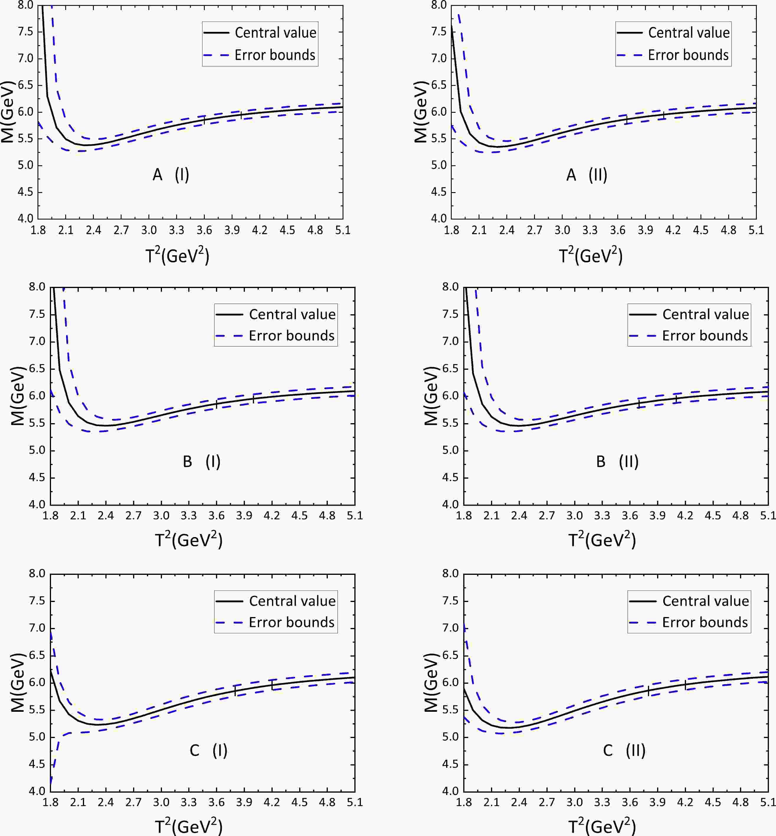
$ J_{(\mu)}(x) $ and$ \eta_{(\mu)} (x) $ are less than$0.02\,\;\rm{GeV}$ if the same parameters are set. Slightly changing the Borel windows$ T^2 $ or continuum threshold parameters$ s_0 $ is sufficient to smear the differences between the outcomes of the partial and covariant derivatives. From Tables 1 and 2, we found that if we set the same pole contributions, then the central values of the baryon masses remain essentially unchanged while those of the pole residues change slightly. Another interesting point is that the contributions of the perturbative terms for currents$ \eta_{(\mu)} (x) $ with covariant derivatives are smaller than those from currents$ J_{(\mu)}(x) $ with partial derivatives. The currents with covariant derivatives are gauge covariant/ invariant; however, this disfavors the interpretation of the covariant derivatives as angular momenta in the non-relativistic limit, i.e.,$ D \to \vec{p}+g_s\vec{G} $ , while the currents with partial derivatives are not gauge covariant, which favors the interpretation of the partial derivatives as angular momenta in the non-relativistic limit, i.e.,$ \partial \to \vec{p} $ . If only the baryon masses are concerned, we can choose either currents$ J_{(\mu)}(x) $ or$ \eta_{(\mu)} (x) $ .Figures 1 and 2 plot the variation trends of the baryon masses with the Borel parameters; the two vertical lines indicate the ranges of the Borel platforms. In Table 2, we show the baryon masses and pole residues explicitly by accounting for all uncertainties of the input parameters. Note that the currents containing both covariant and partial derivatives can lead to baryon masses consistent with experimental data.
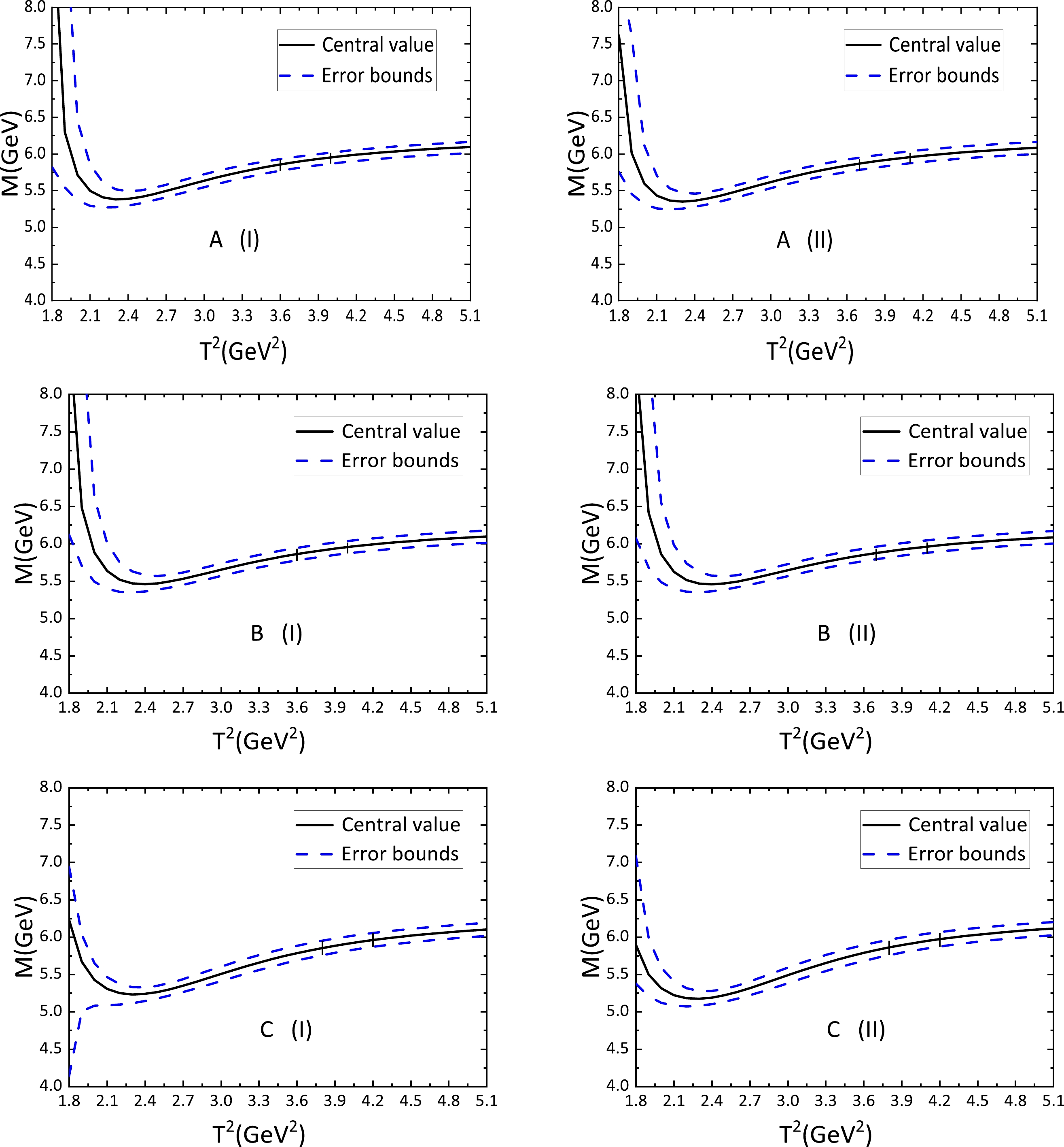
Figure 1. (color online) Masses of the
${\Lambda_b}({{1}/{2}^-})$ ,${\Lambda_b}({3}/{2}^-,1)$ and${\Lambda_b}({3}/{2}^-,2)$ states (labeled as A, B, and C, respectively) with variations of the Borel parameters$ T^2 $ , where (I) and (II) denote the currents with partial and covariant derivatives, respectively.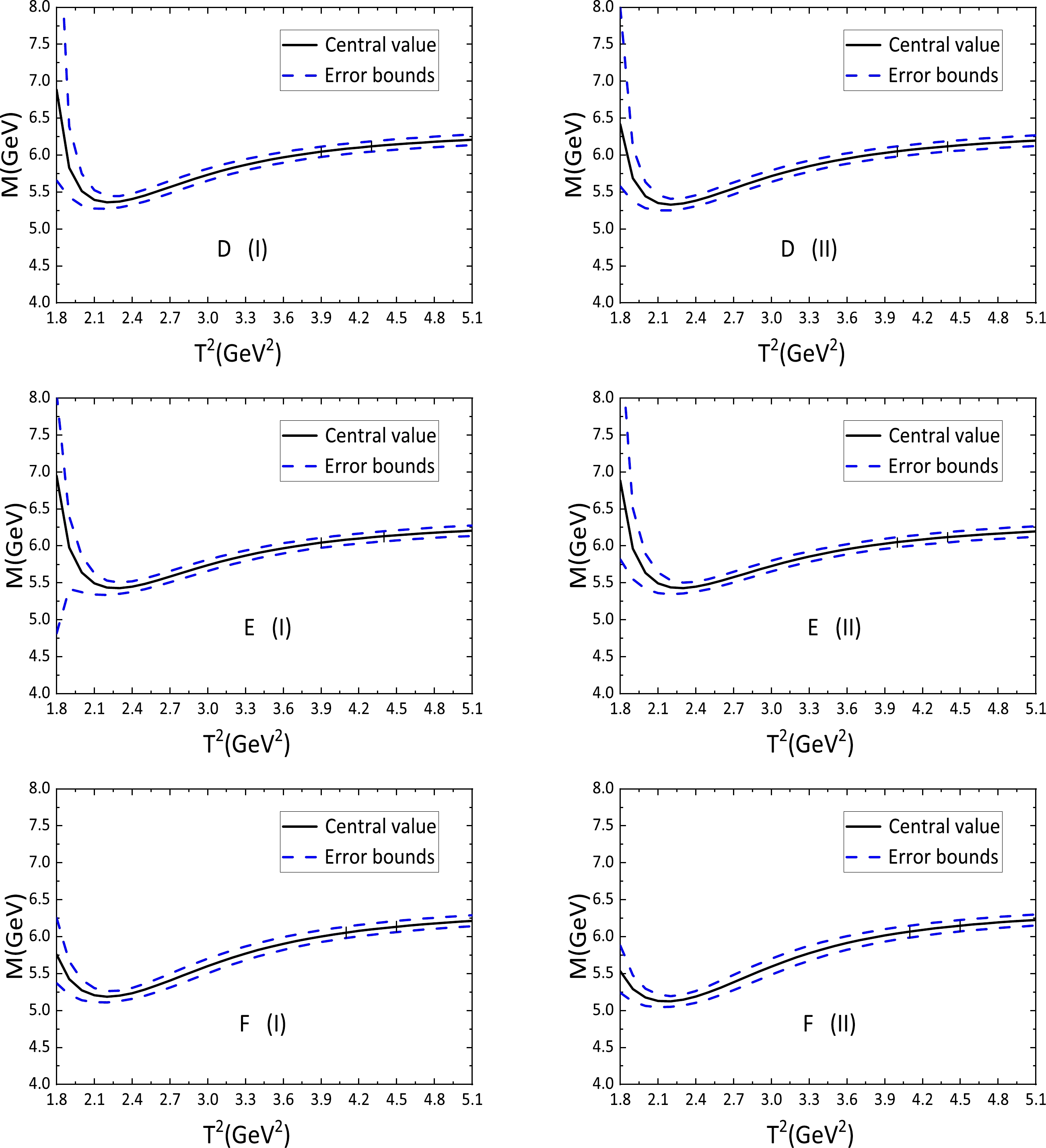
Figure 2. (color online) Masses of the
${\Xi_b}({{1}/{2}^-})$ ,${\Xi_b}({3}/{2}^-,1)$ and${\Xi_b}({3}/{2}^-,2)$ states (labeled as D, E, and F, respectively) with variations of the Borel parameters$ T^2 $ , where (I) and (II) denote the currents with partial and covariant derivatives, respectively.The predicted masses from the currents with partial (covariant) derivatives were
$ M_{-}=5.91 {\pm0.13}\;\rm{GeV} $ ($5.91 {\pm 0.13} \; \rm{GeV}$ ),$ 5.91 {\pm0.14}\; \rm{GeV} $ ($ 5.91 {\pm0.13}\; \rm{GeV} $ ), and$5.92 {\pm0.15} \rm{GeV}$ ($ 5.92 {\pm0.15}\; \rm{GeV} $ ), which are consistent with the experimentally measured masses$M_{\Lambda_b(5912)}=5911.97\pm 0.12 \pm 0.02 \pm 0.66 ~\rm{ MeV}$ or$M_{\Lambda_b(5920)} =5919.77 \pm0.08 \pm 0.02 \pm 0.66 {\rm MeV}$ from the LHCb collaboration [3]. The numerical results indicate that$ \Lambda_b(5912) $ and$ \Lambda_b(5920) $ could be the Λ-type P-wave bottom baryon states with$J^P={1}/{2}^-$ and${3}/{2}^-$ , respectively. Analogously, the predicted masses$ M=6.10 {\pm0.11}\,\rm{GeV} $ ($ 6.09 {\pm0.11}\,\rm{GeV} $ ),$ 6.10 {\pm0.10}\; \rm{GeV} $ ($ 6.10 {\pm0.10}\; \rm{GeV} $ ) and$6.11 {\pm0.12} \; \rm{GeV}$ ($ 6.12 {\pm0.13}\; \rm{GeV} $ ) are consistent with the experimentally measured masses$M_{\Xi_b(6087)} = $ $6087.24\pm0.2 \pm0.06 \pm 0.5\; \rm{ MeV}$ ,$ M_{\Xi_b(6095)}= $ $ 6095.26 \pm0.15 \pm0.03 \pm0.5\; \rm{ MeV}$ , or$M_{\Xi_b(6100)}=6099.74\pm 0.11\pm0.02\pm 0.6 \; \rm{ MeV}$ from the LHCb collaboration [12]. Our numerical results indicate that$ \Xi_b(6087) $ and$ \Xi_b(6095/6100) $ could be the Λ-type P-wave bottom baryon states with$J^P={1}/{2}^-$ and${3}/{2}^-$ , respectively.$ \Lambda_b(5920) $ and$ \Xi_b(6095/6100) $ could be interpreted to have at least two remarkable under-structures or Fock components.We cannot assign those bottom baryon states unambiguously with the masses alone; at least the dominant strong decays should be investigated, such as
$ \begin{aligned}[b] \Xi_b^0(6087) \to& \Xi_b^{\prime-}\pi^+/\Xi_b^{0}\rho^0 \to \Xi_b^0 \pi^-\pi^+\, , \\ \Xi_b^-(?)\to& \Xi_b^{\prime0}\pi^-/\Xi_b^-\rho^0 \to \Xi_b^-\pi^+\pi^-\, , \\ \Xi_b^0(6095)\to& \Xi_b^{*-}\pi^+/\Xi_b^{0}\rho^0 \to \Xi_b^0\pi^-\pi^+\, , \\ \Xi_b^-(6100)\to& \Xi_b^{*0}\pi^- /\Xi_b^-\rho^0\to \Xi_b^-\pi^+\pi^-\, , \end{aligned} $

(23) $ \begin{aligned}[b] \Lambda_b^0(5912) \to& \Sigma_b^-\pi^+/\Lambda_b^{0}\rho^0 \to \Lambda_b^0 \pi^-\pi^+\, , \\ \Lambda_b^0(5920) \to& \Sigma_b^{*-}\pi^+/\Lambda_b^{0}\rho^0 \to \Lambda_b^0 \pi^-\pi^+\, , \end{aligned} $

(24) where intermediate
$ \rho^0 $ is off-shell, and$ \Xi_b^{\prime0} $ is also off-shell as the decay$ \Xi_b^{\prime0}\to \Xi_b^-\pi^+ $ is kinematically forbidden. At the present time, there only exist experimental evidences for the isospin doublet$(\Xi_b^0(6095),\;\Xi_b^-(6100))$ ; there are no experimental evidences for the isospin doublet$(\Xi_b^0(6087), \;\Xi_b^-(?))$ . We can explore these three-body decays with the (light-cone) QCD sum rules directly or indirectly [21, 38, 63], and then compare the predictions with experimental data to diagnose the nature of those P-wave baryon states. This will be addressed in future studies. -
In this study, we extend previous studies of ours to comprehensively explore the Λ-type P-wave bottom baryon states with the QCD sum rules. We introduce a relative P-wave between the two light quarks in the diquarks to construct the interpolating currents, and refer to them as Λ-type currents because the two light quarks are antisymmetric. We carry out the expansion of the operator product up to the vacuum condensates of dimension 10 in a self-consistent way, obtain the spectral representations through dispersion relation, distinguish the contributions of the negative-parity and positive-parity bottom baryon states unambiguously, and determine the ideal energy scales of the QCD spectral densities using the modified energy scale formula by considering the light-flavor
$S U(3)$ breaking effects. Our numerical results support the assignment of$ \Lambda^0_b(5912) $ and$ \Xi_b^0(6087) $ to the Λ-type P-wave baryon states with spin-parity$J^P={1}/{2}^-$ and valence quarks$ udb $ and$ usb $ , respectively, and assignment of$ \Lambda^0_b(5920) $ and$ \Xi^0_b(6095) $ ($ \Xi^-_b(6100) $ ) to the Λ-type P-wave baryon states with spin-parity$J^P={3}/{2}^-$ and valence quarks$ udb $ and$ usb $ ($ dsb $ ), respectively.$ \Xi^0_b(6095) $ and$ \Xi^-_b(6100) $ form an isospin doublet, while the isospin partner of$ \Xi_b^0(6087) $ has not been observed yet.$ \Xi_b(6095) $ and$ \Xi_b(6100) $ may have two structures or Fock components, given that there exist two$J^P={3}/{2}^-$ currents with different structures but exhibiting potential coupling to the bottom baryon states with almost degenerated masses. Furthermore, we observe that the currents with covariant or partial derivatives lead to almost the same baryon masses; if only the baryon masses are considered, we can choose either covariant or partial derivatives for the construction of the currents. According to the quantum field theory, we constructed gauge invariant currents with the same quantum numbers as the hadrons to interpolate them; therefore, covariant derivatives are preferred. -
The QCD spectral densities
$\rho_{j,\rm QCD}^0(s)$ and$\rho_{j,\rm QCD}^1(s)$ for the currents with the partial derivatives are$ \begin{aligned}[b] \\ \rho_{j,\rm QCD}^0(s)=&\rho_{\frac{1}{2},\Lambda_b}^0(s)\, ,\,\, \rho_{\frac{3}{2},1,\Lambda_b}^0(s)\, , \, \,\rho_{\frac{3}{2},2,\Lambda_b}^0(s)\, , \, \,\rho_{\frac{1}{2},\Xi_b}^0(s)\, ,\,\, \rho_{\frac{3}{2},1,\Xi_b}^0(s)\, , \, \,\rho_{\frac{3}{2},2,\Xi_b}^0(s)\, , \\ \rho_{j,\rm QCD}^1(s)=&\rho_{\frac{1}{2},\Lambda_b}^1(s)\, ,\,\, \rho_{\frac{3}{2},1,\Lambda_b}^1(s)\, , \, \,\rho_{\frac{3}{2},2,\Lambda_b}^1(s)\, , \, \,\rho_{\frac{1}{2},\Xi_b}^1(s)\, ,\,\, \rho_{\frac{3}{2},1,\Xi_b}^1(s)\, , \, \,\rho_{\frac{3}{2},2,\Xi_b}^1(s)\, , \end{aligned} \tag{A1}$ 
where
$ j=\dfrac{1}{2} $ ,$ \dfrac{3}{2} $ ,$ \begin{aligned}[b] \rho_{\frac{1}{2},\Lambda_b}^0(s)=&\rho_{\frac{1}{2},\Xi_b}^0(s)\mid_{m_s \to 0, \langle\bar{s}s\rangle \to\langle\bar{q}q\rangle, \langle\bar{s}g_s\sigma Gs\rangle \to\langle\bar{q}g_s\sigma Gq\rangle} \, , \\ \rho_{\frac{3}{2},1,\Lambda_b}^0(s)=&\rho_{\frac{3}{2},1,\Xi_b}^0(s)\mid_{m_s \to 0, \langle\bar{s}s\rangle \to\langle\bar{q}q\rangle, \langle\bar{s}g_s\sigma Gs\rangle \to\langle\bar{q}g_s\sigma Gq\rangle} \, , \\ \rho_{\frac{3}{2},2,\Lambda_b}^0(s)=&\rho_{\frac{3}{2},2,\Xi_b}^0(s)\mid_{m_s \to 0, \langle\bar{s}s\rangle \to\langle\bar{q}q\rangle, \langle\bar{s}g_s\sigma Gs\rangle \to\langle\bar{q}g_s\sigma Gq\rangle}\, , \end{aligned}\tag{A2} $

$ \begin{aligned}[b] \rho_{\frac{1}{2},\Lambda_b}^1(s)=&\rho_{\frac{1}{2},\Xi_b}^1(s)\mid_{m_s \to 0, \langle\bar{s}s\rangle \to\langle\bar{q}q\rangle, \langle\bar{s}g_s\sigma Gs\rangle \to\langle\bar{q}g_s\sigma Gq\rangle} \, , \\ \rho_{\frac{3}{2},1,\Lambda_b}^1(s)=&\rho_{\frac{3}{2},1,\Xi_b}^1(s)\mid_{m_s \to 0, \langle\bar{s}s\rangle \to\langle\bar{q}q\rangle, \langle\bar{s}g_s\sigma Gs\rangle \to\langle\bar{q}g_s\sigma Gq\rangle} \, , \\ \rho_{\frac{3}{2},2,\Lambda_b}^1(s)=&\rho_{\frac{3}{2},2,\Xi_b}^1(s)\mid_{m_s \to 0, \langle\bar{s}s\rangle \to\langle\bar{q}q\rangle, \langle\bar{s}g_s\sigma Gs\rangle \to\langle\bar{q}g_s\sigma Gq\rangle}\, , \end{aligned}\tag{A3} $

$ \begin{aligned}[b] \rho^0_{\frac{1}{2},\Xi_b}(s)=&\frac{m_b} {32\pi^4} \int_{x_i}^{1}{\rm d} x(1-x)^3({s-\tilde{m}_b^2})^3-\frac{m_b^3} {96\pi^2} \langle\frac{\alpha_{s}GG}{\pi}\rangle\int_{x_i}^{1}{\rm d}x\frac{(1-x)^3}{x^3}\\&+\frac{m_b} {32\pi^2} \langle\frac{\alpha_{s}GG}{\pi}\rangle\int_{x_i}^{1}{\rm d}x\frac{(x-1)(x+1)(3x-2)}{x^2}(s-\tilde{m}_b^2)\\ &+m_sm_b\langle\bar{s}s\rangle\langle\frac{\alpha_{s}GG}{\pi}\rangle\int_{x_i}^{1}dx\frac{1}{32x}\delta(s-\tilde{m}_b^2)+\frac{m_sm_b(5\langle\bar{s}g_s\sigma Gs\rangle-12\langle\bar{q}g_s\sigma Gq\rangle)}{32\pi^2}\int_{x_i}^{1}{\rm d}x\\ & +\frac{m_b(\langle\bar{q}q\rangle\langle\bar{s}g_s\sigma Gs\rangle+\langle\bar{s}s\rangle\langle\bar{q}g_s\sigma Gq\rangle)}{4}\delta(s-m_b^2)-\frac{m_b\langle\bar{s}g_s\sigma Gs\rangle\langle\bar{q}g_s\sigma Gq\rangle}{48T^2}\left(-2+\frac{3s}{T^2}\right)\delta(s-m_b^2) \, , \end{aligned}\tag{A4} $

$ \begin{aligned}[b] \rho^1_{\frac{1}{2},\Xi_b}(s)=&\frac{1} {16\pi^4} \int_{x_i}^{1}{\rm d}xx(1-x)^3({s-\tilde{m}_b^2})^3+\frac{3m_s(2\langle\bar{s}s\rangle-\langle\bar{q}q\rangle)} {4\pi^2}\int_{x_i}^{1}{\rm d}xx(1-x)(s-\tilde{m}_b^2)\\ &-\frac{m_b^2} {48\pi^2} \langle\frac{\alpha_{s}GG}{\pi}\rangle\int_{x_i}^{1}{\rm d}x\frac{(1-x)^3}{x^2}+\frac{3}{64\pi^2}\langle\frac{\alpha_{s}GG}{\pi}\rangle\int_{x_i}^{1}{\rm d}x(1-x)^2(s-\tilde{m}_b^2) \\ &+\frac{m_sm_b^2(\langle\bar{q}q\rangle-2\langle\bar{s}s\rangle)}{24 T^2}\langle\frac{\alpha_{s}GG}{\pi}\rangle\int_{x_i}^{1}{\rm d}x\frac{(1-x)}{x^2}\delta(s-\tilde{m}_b^2)+\frac{m_s\langle\bar{s}s\rangle}{32}\langle\frac{\alpha_{s}GG}{\pi}\rangle\int_{x_i}^{1}{\rm d}x\delta(s-\tilde{m}_b^2)\\ &+\frac{m_s\langle\bar{q}q\rangle} {48} \langle\frac{\alpha_{s}GG}{\pi}\rangle\delta(s-m_b^2)+\frac{m_s\langle\bar{q}g_s\sigma Gq\rangle} {16\pi^2}\int_{x_i}^{1}{\rm d}x(7x-1)-\frac{11m_s\langle\bar{s}g_s\sigma Gs\rangle}{32\pi^2}\int_{x_i}^{1}{\rm d}xx\\ &-\frac{\langle\bar{s}g_s\sigma Gs\rangle\langle\bar{q}g_s\sigma Gq\rangle}{16T^2}\left(1+\frac{s}{T^2}\right)\delta(s-m_b^2) \, , \end{aligned}\tag{A5} $

$ \begin{aligned}[b] \rho^0_{\frac{3}{2},1,\Xi_b}(s)=&\frac{m_b} {128\pi^4} \int_{x_i}^{1}{\rm d}x(1-x)^3({s-\tilde{m}_b^2})^3-\frac{m_b^3} {384\pi^2} \langle\frac{\alpha_{s}GG}{\pi}\rangle\int_{x_i}^{1}{\rm d}x\frac{(1-x)^3}{x^3}-\frac{m_b}{576\pi^2} \langle\frac{\alpha_{s}GG}{\pi}\rangle\int_{x_i}^{1}{\rm d}x\frac{(1-x)^3}{x}(-3s+2\tilde{m}_b^2)\\ &-\frac{m_b} {768\pi^2} \langle\frac{\alpha_{s}GG}{\pi}\rangle\int_{x_i}^{1}{\rm d}x\frac{(x-1)(6-13x+x^2)}{x^2}(s-\tilde{m}_b^2)\\&-\frac{m_sm_b\langle\bar{s}s\rangle}{384}\langle\frac{\alpha_{s}GG}{\pi}\rangle\int_{x_i}^{1}{\rm d}x\left[\frac{3-4x}{x}-\frac{4(x-1)}{x}\frac{s}{T^2}\right]\delta(s-\tilde{m}_b^2)\\ &+\frac{5m_sm_b\langle\bar{s}g_s\sigma Gs\rangle}{128\pi^2}\int_{x_i}^{1}{\rm d}x+\frac{m_sm_b\langle\bar{q}g_s\sigma Gq\rangle}{192\pi^2}\int_{x_i}^{1}{\rm d}x(x-19)+\frac{m_sm_b\langle\bar{q}g_s\sigma Gq\rangle}{96\pi^2}\int_{x_i}^{1}{\rm d}x\frac{s(1-x)^2}{x}\delta(s-\tilde{m}_b^2)\\ &+\frac{m_b(\langle\bar{q}q\rangle\langle\bar{s}g_s\sigma Gs\rangle+\langle\bar{s}s\rangle\langle\bar{q}g_s\sigma Gq\rangle)}{16}\delta(s-m_b^2)-\frac{m_b\langle\bar{s}g_s\sigma Gs\rangle\langle\bar{q}g_s\sigma Gq\rangle}{256}\delta(s-m_b^2) \, , \end{aligned}\tag{A6} $

$ \begin{aligned}[b] \rho^1_{\frac{3}{2},1,\Xi_b}(s)=&\frac{1} {64\pi^4} \int_{x_i}^{1}{\rm d}xx(1-x)^3({s-\tilde{m}_b^2})^3-\frac{3m_s(2\langle\bar{q}q\rangle-2\langle\bar{s}s\rangle)} {16\pi^2}\int_{x_i}^{1}{\rm d}xx(1-x)(s-\tilde{m}_b^2)\\ &-\frac{m_b^2} {192\pi^2} \langle\frac{\alpha_{s}GG}{\pi}\rangle\int_{x_i}^{1}{\rm d}x\frac{(1-x)^3}{x^2}-\frac{1}{256\pi^2}\langle\frac{\alpha_{s}GG}{\pi}\rangle\int_{x_i}^{1}{\rm d}x(1-x)^2(s-\tilde{m}_b^2)\\ &+\frac{m_sm_b^2(\langle\bar{q}q\rangle-2\langle\bar{s}s\rangle)}{96 T^2}\langle\frac{\alpha_{s}GG}{\pi}\rangle\int_{x_i}^{1}{\rm d}x(1-x)\delta(s-\tilde{m}_b^2)-\frac{m_s\langle\bar{s}s\rangle}{384}\langle\frac{\alpha_{s}GG}{\pi}\rangle\int_{x_i}^{1}{\rm d}x\delta(s-\tilde{m}_b^2) \\ &+\frac{m_s\langle\bar{q}q\rangle} {192} \langle\frac{\alpha_{s}GG}{\pi}\rangle\delta(s-m_b^2) +\frac{m_s\langle\bar{q}g_s\sigma Gq\rangle} {384\pi^2}\int_{x_i}^{1}{\rm d}x(2+x)-\frac{11m_s\langle\bar{s}g_s\sigma Gs\rangle}{128\pi^2}\int_{x_i}^{1}{\rm d}xx\\ &-\frac{3\langle\bar{s}g_s\sigma Gs\rangle\langle\bar{q}g_s\sigma Gq\rangle}{64T^2}\left(1-\frac{s}{T^2}\right)\delta(s-m_b^2) \, , \end{aligned}\tag{A7} $

$ \begin{aligned}[b] \rho^0_{\frac{3}{2},2,\Xi_b}(s)=&\frac{m_b} {192\pi^4} \int_{x_i}^{1}{\rm d}x(4+x)(1-x)^3(s-\tilde{m}_b^2)^3+\frac{m_sm_b(\langle\bar{s}s\rangle-2\langle\bar{q}q\rangle)}{8\pi^2}\int_{x_i}^{1}{\rm d}xx(1-x)(s-\tilde{m}_b^2)\\ &+\frac{m_b^3}{576\pi^2}\langle\frac{\alpha_{s}GG}{\pi}\rangle\int_{x_i}^{1}{\rm d}x\frac{(x-1)^3(4+x)} {x^3}-\frac{m_b}{192\pi^2}\langle\frac{\alpha_{s}GG}{\pi}\rangle\int_{x_i}^{1}{\rm d}x\frac{(x-1)^3(4+x)} {x^2}(s-\tilde{m}_b^2)\\ &+\frac{m_b}{384\pi^2}\langle\frac{\alpha_{s}GG}{\pi}\rangle\int_{x_i}^{1}{\rm d}x\frac{(x-1)[s(24-51x+44x^2)+(-10+23x-30x^2)\tilde{m}_b^2]}{x}\\ &+\frac{m_sm_b(\langle\bar{s}s\rangle-2\langle\bar{q}q\rangle)}{48}\langle\frac{\alpha_{s}GG}{\pi}\rangle\int_{x_i}^{1}{\rm d}x\frac{(1-x)(3x-1)}{3x^2}\delta(s-\tilde{m}_b^2)\\ &-\frac{m_sm_b\langle\bar{q}q\rangle}{72}\langle\frac{\alpha_{s}GG}{\pi}\rangle\int_{x_i}^{1}{\rm d}x\delta(s-\tilde{m}_b^2)+\frac{m_sm_b\langle\bar{q}q\rangle}{144}\langle\frac{\alpha_{s}GG}{\pi}\rangle\delta(s-m_b^2) \end{aligned} $

$ \begin{aligned}[b] &+\frac{m_sm_b\langle\bar{s}s\rangle}{288}\langle\frac{\alpha_{s}GG}{\pi}\rangle\int_{x_i}^{1}{\rm d}x\left(1+\frac{x-1}{x}\frac{s}{T^2}\right)\delta(s-\tilde{m}_b^2)+\frac{7m_sm_b\langle\bar{q}g_s\sigma Gq\rangle}{96\pi^2}\int_{x_i}^{1}{\rm d}x\frac{s(1-x)^2}{x}\delta(s-\tilde{m}_b^2)\\ &+\frac{m_sm_b\langle\bar{s}g_s\sigma Gs\rangle}{384\pi^2}\int_{x_i}^{1}{\rm d}x(81-64x)+\frac{m_sm_b\langle\bar{q}g_s\sigma Gq\rangle}{384\pi^2}\int_{x_i}^{1}{\rm d}x(-842+782x)\\ &+\frac{3m_b(\langle\bar{q}q\rangle\langle\bar{s}g_s\sigma Gs\rangle+\langle\bar{s}s\rangle\langle\bar{q}g_s\sigma Gq\rangle)}{16}\delta(s-m_b^2)-\frac{m_b\langle\bar{s}g_s\sigma Gs\rangle\langle\bar{q}g_s\sigma Gq\rangle}{96T^2}\left(-7+\frac{13s}{2T^2}\right)\delta(s-m_b^2) \, , \end{aligned}\tag{A8} $

$ \begin{aligned}[b] \rho^1_{\frac{3}{2},2,\Xi_b}(s)=&\frac{1} {64\pi^4} \int_{x_i}^{1}{\rm d}xx(2+x)(1-x)^3(s-\tilde{m}_b^2)^3+\frac{m_b^2} {192\pi^2} \langle\frac{\alpha_{s}GG}{\pi}\rangle\int_{x_i}^{1}{\rm d}x\frac{(x-1)^3(2+x)}{x^2}\\ &+\frac{m_s\langle\bar{q}q\rangle}{8\pi^2}\int_{x_i}^{1}{\rm d}xx(x-1)(x+3)(s-\tilde{m}_b^2)+\frac{m_s\langle\bar{q}q\rangle}{72}\langle\frac{\alpha_{s}GG}{\pi}\rangle\delta(s-m_b^2)\\ &-\frac{m_s\langle\bar{s}s\rangle}{8\pi^2}\int_{x_i}^{1}{\rm d}xx(x-1)(8x-1)(s-\tilde{m}_b^2)+\langle\frac{\alpha_{s}GG}{\pi}\rangle\int_{x_i}^{1}{\rm d}x\frac{(1-x)(20-34x-13x^2)}{1152\pi^2}(s-\tilde{m}_b^2)\\ &-\frac{m_sm_b^2\langle\bar{s}s\rangle}{144T^2}\langle\frac{\alpha_{s}GG}{\pi}\rangle\int_{x_i}^{1}{\rm d}x\frac{(1-x)(8x-1)}{x^2}\delta(s-\tilde{m}_b^2)-\frac{m_sm_b^2\langle\bar{q}q\rangle}{144T^2}\langle\frac{\alpha_{s}GG}{\pi}\rangle\int_{x_i}^{1}{\rm d}x\frac{(x-1)(x+3)}{x^2}\delta(s-\tilde{m}_b^2)\\ &-\frac{m_s\langle\bar{q}q\rangle}{144}\langle\frac{\alpha_{s}GG}{\pi}\rangle\int_{x_i}^{1}{\rm d}xx\delta(s-\tilde{m}_b^2)+\frac{5m_s\langle\bar{s}s\rangle}{576}\langle\frac{\alpha_{s}GG}{\pi}\rangle\int_{x_i}^{1}{\rm d}xx\delta(s-\tilde{m}_b^2)\\ &-\frac{m_s\langle\bar{s}g_s\sigma Gs\rangle}{128\pi^2}\int_{x_i}^{1}{\rm d}xx(68x-47)+\frac{m_s\langle\bar{q}g_s\sigma Gq\rangle}{192\pi^2}\int_{x_i}^{1}{\rm d}xx(29x-11)\\ &+\frac{5(\langle\bar{q}q\rangle\langle\bar{s}g_s\sigma Gs\rangle+\langle\bar{s}s\rangle\langle\bar{q}g_s\sigma Gq\rangle)}{48}\delta(s-m_b^2)+\frac{\langle\bar{s}g_s\sigma Gs\rangle\langle\bar{q}g_s\sigma Gq\rangle}{576T^2}\left(37-\frac{13s}{3T^2}\right)\delta(s-m_b^2) \, , \end{aligned}\tag{A9} $

where
$ \tilde{m}_b^2=\dfrac{{m}_b^2}{x} $ ,$ x_i=\dfrac{{m}_b^2}{s} $ .With the following simple replacements,
$ \begin{aligned}[b] \rho_{j,\rm QCD}^0(s)\to&\rho_{j,\rm QCD}^0(s)+\tilde{\rho}^0_{j,\rm QCD}(s)\, , \\ \rho_{j,\rm QCD}^1(s)\to&\rho_{j,\rm QCD}^1(s)+\tilde{\rho}^1_{j,\rm QCD}(s)\, , \end{aligned} \tag{A10}$

we obtain the corresponding QCD spectral densities for the currents with covariant derivatives, with the corresponding additional terms:
$ \begin{aligned}[b] \tilde{\rho}_{j,\rm QCD}^0(s)=&\tilde{\rho}_{\frac{1}{2},\Lambda_b}^0(s)\, ,\,\, \tilde{\rho}_{\frac{3}{2},1,\Lambda_b}^0(s)\, , \, \,\tilde{\rho}_{\frac{3}{2},2,\Lambda_b}^0(s)\, , \, \,\tilde{\rho}_{\frac{1}{2},\Xi_b}^0(s)\, ,\,\, \tilde{\rho}_{\frac{3}{2},1,\Xi_b}^0(s)\, , \, \,\tilde{\rho}_{\frac{3}{2},2,\Xi_b}^0(s)\, , \\ \tilde{\rho}_{j,\rm QCD}^1(s)=&\tilde{\rho}_{\frac{1}{2},\Lambda_b}^1(s)\, ,\,\, \tilde{\rho}_{\frac{3}{2},1,\Lambda_b}^1(s)\, , \, \,\tilde{\rho}_{\frac{3}{2},2,\Lambda_b}^1(s)\, , \, \,\rho_{\frac{1}{2},\Xi_b}^1(s)\, ,\,\, \tilde{\rho}_{\frac{3}{2},1,\Xi_b}^1(s)\, , \, \,\tilde{\rho}_{\frac{3}{2},2,\Xi_b}^1(s)\, , \end{aligned}\tag{A11} $

$ \begin{aligned}[b] \tilde{\rho}_{\frac{1}{2},\Lambda_b}^0(s)=&\tilde{\rho}_{\frac{1}{2},\Xi_b}^0(s)\mid_{m_s \to 0, \langle\bar{s}s\rangle \to\langle\bar{q}q\rangle, \langle\bar{s}g_s\sigma Gs\rangle \to\langle\bar{q}g_s\sigma Gq\rangle} \, , \\ \tilde{\rho}_{\frac{3}{2},1,\Lambda_b}^0(s)=&\tilde{\rho}_{\frac{3}{2},1,\Xi_b}^0(s)\mid_{m_s \to 0, \langle\bar{s}s\rangle \to\langle\bar{q}q\rangle, \langle\bar{s}g_s\sigma Gs\rangle \to\langle\bar{q}g_s\sigma Gq\rangle} \, , \\ \tilde{\rho}_{\frac{3}{2},2,\Lambda_b}^0(s)=&\tilde{\rho}_{\frac{3}{2},2,\Xi_b}^0(s)\mid_{m_s \to 0, \langle\bar{s}s\rangle \to\langle\bar{q}q\rangle, \langle\bar{s}g_s\sigma Gs\rangle \to\langle\bar{q}g_s\sigma Gq\rangle}\, , \end{aligned}\tag{A12} $

$ \begin{aligned}[b] \tilde{\rho}_{\frac{1}{2},\Lambda_b}^1(s)=&\tilde{\rho}_{\frac{1}{2},\Xi_b}^1(s)\mid_{m_s \to 0, \langle\bar{s}s\rangle \to\langle\bar{q}q\rangle, \langle\bar{s}g_s\sigma Gs\rangle \to\langle\bar{q}g_s\sigma Gq\rangle} \, , \\ \tilde{\rho}_{\frac{3}{2},1,\Lambda_b}^1(s)=&\tilde{\rho}_{\frac{3}{2},1,\Xi_b}^1(s)\mid_{m_s \to 0, \langle\bar{s}s\rangle \to\langle\bar{q}q\rangle, \langle\bar{s}g_s\sigma Gs\rangle \to\langle\bar{q}g_s\sigma Gq\rangle} \, , \\ \tilde{\rho}_{\frac{3}{2},2,\Lambda_b}^1(s)=&\tilde{\rho}_{\frac{3}{2},2,\Xi_b}^1(s)\mid_{m_s \to 0, \langle\bar{s}s\rangle \to\langle\bar{q}q\rangle, \langle\bar{s}g_s\sigma Gs\rangle \to\langle\bar{q}g_s\sigma Gq\rangle}\, , \end{aligned}\tag{A13} $

$ \begin{aligned}[b] \tilde{\rho}^0_{\frac{1}{2},\Xi_b}(s)=&\frac{3m_b} {64\pi^2} \langle\frac{\alpha_{s}GG}{\pi}\rangle\int_{x_i}^{1}{\rm d} x(1-x)(s-\tilde{m}_b^2)+\frac{m_sm_b\langle\bar{s}s\rangle}{64}\langle\frac{\alpha_{s}GG}{\pi}\rangle\delta(s-m_b^2)\\ &+\frac{3m_sm_b\langle\bar{q}g_s\sigma Gq\rangle}{64\pi^2}\int_{x_i}^{1}{\rm d}x-\frac{m_bs\langle\bar{s}g_s\sigma Gs\rangle\langle\bar{q}g_s\sigma Gq\rangle}{32T^4}\delta(s-m_b^2) \, , \end{aligned}\tag{A14} $

$ \begin{aligned}[b] \tilde{\rho}^1_{\frac{1}{2},\Xi_b}(s)=&\frac{3} {64\pi^2}\langle\frac{\alpha_{s}GG}{\pi}\rangle\int_{x_i}^{1}{\rm d}xx(1-x)(s-\tilde{m}_b^2)+\frac{m_s\langle\bar{s}s\rangle}{64}\langle\frac{\alpha_{s}GG}{\pi}\rangle\delta(s-m_b^2)\\ &-\frac{3m_s\langle\bar{s}g_s\sigma Gs\rangle}{64\pi^2}\int_{x_i}^{1}{\rm d}xx+\frac{\langle\bar{s}g_s\sigma Gs\rangle\langle\bar{q}g_s\sigma Gq\rangle}{32T^2}\left(1+\frac{s}{T^2}\right)\delta(s-m_b^2) \, , \end{aligned}\tag{A15} $

$ \begin{aligned}[b] \tilde{\rho}^0_{\frac{3}{2},1,\Xi_b}(s)=&\frac{m_b} {256\pi^2} \langle\frac{\alpha_{s}GG}{\pi}\rangle\int_{x_i}^{1}{\rm d}x(1-x)(s-\tilde{m}_b^2)+\frac{m_sm_b\langle\bar{s}s\rangle}{256}\langle\frac{\alpha_{s}GG}{\pi}\rangle\delta(s-m_b^2)+\frac{3m_sm_b\langle\bar{q}g_s\sigma Gq\rangle}{256\pi^2}\int_{x_i}^{1}{\rm d}x\\ &-\frac{m_bs\langle\bar{s}g_s\sigma Gs\rangle\langle\bar{q}g_s\sigma Gq\rangle}{128T^4}\delta(s-m_b^2) \, , \end{aligned}\tag{A16} $

$ \begin{aligned}[b] \tilde{\rho}^1_{\frac{3}{2},1,\Xi_b}(s)=&\frac{1} {256\pi^2} \langle\frac{\alpha_{s}GG}{\pi}\rangle\int_{x_i}^{1}{\rm d}xx(1-x)(1+2x)(s-\tilde{m}_b^2) \\ &-\frac{m_s\langle\bar{s}s\rangle}{192}\langle\frac{\alpha_{s}GG}{\pi}\rangle\int_{x_i}^{1}{\rm d}xx\delta(s-\tilde{m}_b^2)+\frac{m_s\langle\bar{s}s\rangle}{256}\langle\frac{\alpha_{s}GG}{\pi}\rangle\delta(s-m_b^2)\\ &+\frac{m_s\langle\bar{s}g_s\sigma Gs\rangle}{256\pi^2}\int_{x_i}^{1}{\rm d}xx(1-4x)-\frac{\langle\bar{s}g_s\sigma Gs\rangle\langle\bar{q}g_s\sigma Gq\rangle}{128T^2}\left(\frac{1}{3}-\frac{s}{T^2}\right)\delta(s-m_b^2) \, , \end{aligned}\tag{A17} $

$ \begin{aligned}[b] \tilde{\rho}^0_{\frac{3}{2},2,\Xi_b}(s)=&\frac{m_b} {256\pi^2} \langle\frac{\alpha_{s}GG}{\pi}\rangle\int_{x_i}^{1}{\rm d}x(x-1)(9+4x)(s-\tilde{m}_b^2) \\ &+\frac{m_sm_b\langle\bar{s}s\rangle}{96}\langle\frac{\alpha_{s}GG}{\pi}\rangle\int_{x_i}^{1}{\rm d}x\delta(s-\tilde{m}_b^2)-\frac{13m_sm_b\langle\bar{s}s\rangle}{768}\langle\frac{\alpha_{s}GG}{\pi}\rangle\delta(s-m_b^2)\\ &+\frac{m_sm_b\langle\bar{q}g_s\sigma Gq\rangle}{256\pi^2}\int_{x_i}^{\rm d}x(8x-13)+\frac{m_b\langle\bar{s}g_s\sigma Gs\rangle\langle\bar{q}g_s\sigma Gq\rangle}{384T^2}\left(\frac{1}{8}+\frac{5s}{T^2}\right)\delta(s-m_b^2) \, , \end{aligned}\tag{A18} $

$ \begin{aligned}[b] \tilde{\rho}^1_{\frac{3}{2},2,\Xi_b}(s)=&\frac{1}{256\pi^2} \langle\frac{\alpha_{s}GG}{\pi}\rangle\int_{x_i}^{1}{\rm d}xx(x-1)(11+2x)(s-\tilde{m}_b^2)\\ &+\frac{m_s\langle\bar{s}s\rangle}{192}\langle\frac{\alpha_{s}GG}{\pi}\rangle\int_{x_i}^{1}{\rm d}xx\delta(s-\tilde{m}_b^2)-\frac{13m_s\langle\bar{s}s\rangle}{768}\langle\frac{\alpha_{s}GG}{\pi}\rangle\delta(s-m_b^2)\\ &+\frac{m_s\langle\bar{q}g_s\sigma Gq\rangle}{256\pi^2}\int_{x_i}^{1}{\rm d}xx(4-x)+\frac{\langle\bar{s}g_s\sigma Gs\rangle\langle\bar{q}g_s\sigma Gq\rangle}{384T^2}\left( 1-\frac{s}{3T^2} \right)\delta(s-m_b^2) \, . \end{aligned}\tag{A19} $

The Λ-type P-wave bottom baryon states via the QCD sum rules
- Received Date: 2023-06-12
- Available Online: 2023-09-15
Abstract: Our study focuses on the Λ-type P-wave bottom baryon states with spin-parity


 DownLoad: