


 Abstract
 HTML
HTML Reference
 Related
 PDF
PDF


-
String theory is one of the most promising grand unified theories. In string theory, the smallest units of nature are not point particles but one dimensional extended strings. Owing to inflation in the early universe, these fundamental strings could have been stretched to cosmological sizes [1]. A cloud of strings is the one-dimensional analog of a cloud of dust. Gurses and Gursey [2] first derived the equations of string motion in general relativity. Later, the solution of Einstein's equation with a string cloud was derived by Letelier [3] and used to establish a star model. Many related papers subsequently considered the string cloud as a fluid in the spacetime background and constructed relevant solutions. The physical properties of these black hole solutions have been investigated [4–9]. For example, for a Schwarzschild black hole with a cloud of strings, the event horizon radius receives a correction of
$ r_h=2M/(1-a) $ , where a is the string cloud parameter [3]. The modification factor$ 1/(1-a) $ may have certain potential astrophysical applications [10, 11].In general, there is always a singularity in the black hole solution, which is enveloped by the event horizon. In contrast, Bardeen proposed a black hole solution without a curvature singularity [12]. Beato and Garcia [13] proposed a magnetic solution of the Einstein equations coupled with nonlinear electrodynamics. Then, several papers studied this type of black hole solution [14–18]. For example, in Ref. [19], the shadow of the Bardeen black hole was calculated and a set of tests was performed on fundamental physics from the shadow of Sgr A*. A Bardeen black hole solution with a cloud of strings was obtained very recently in [17]. Although this black hole solution has the same event horizon characteristic as the regular Bardeen solution, the string parameter a makes the solution singular at the origin. Owing to the significant changes in the properties of black holes, investigating the various intrinsic characteristics of this black hole becomes an interesting topic.
It is well known that one effective way to extract black hole characteristics is to perturb it and observe its response. When considering a perturbation that can be ignored in the spacetime background and choosing an appropriate gauge, the evolution of this perturbation can be described by a series of simple wave equations [20, 21]. Through these perturbation wave equations, we can see that the evolution of perturbation mainly consists of three stages: the initial outburst, quasinormal ringing, and the power law (asymptotically flat spacetime) or exponential (asymptotic de Sitter spacetime) tail [22]. The quasinormal ringing stage, where quasinormal modes (QNMs) are mainly determined by the parameters of the black hole and are independent of the initial perturbation [23, 24], is an important component of current gravitational wave detection [25]. Finally, the third stage is mainly caused by the scattering of perturbations at infinity [26]. This stage is of great significance for studying the stability of black holes. To date, a large number of papers have studied QNMs and power law tails in different spacetime backgrounds using various methods [6, 27–32]. For example, a recent paper [29] studied the QNMs of a Schwarzschild-like black hole with the cosmological constant in conformal Weyl gravity and found that the evolution of the scalar field is divided into three stages: the Schwarzschild ringing stage, effective dark matter ringing stage, and an exponential tail of de Sitter stage. Moreover, [15] analyzed the QNMs of a Bardeen black hole caused by scalar perturbations and compared them with results in the Reissner-Nordstrom black hole.
Given the above motivations, as the first step toward understanding the properties of the Bardeen black hole with a cloud of strings (SBBH), we consider the probe of a massless scalar field over this background and study the properties of its QNM spectra in this paper.
The structure of this paper is as follows. In Sec. II, the metric of the SBBH and scalar perturbation in this background are introduced, and the corresponding effective potential is given. In Sec. III, the methods used to analyze QNMs and greybody factors are introduced, including the finite element method (FEM), WKB approximation, and Prony algorithm. The effects of various parameters on QNMs and greybody factors are calculated for the SBBH in Sec. IV, and the accuracy of the calculations is verified using the Prony method in Sec. V. Finally, some conclusions and corresponding discussions are given in Sec. VI.
-
For the SBBH, the action can be described as general relativity minimally coupled to nonlinear electrodynamics (NED) and string clouds as follows [17]:
$ S=\int {\rm d}^{4} x \sqrt{-g}[R+2 \lambda+{\cal{L}}(F)]+S_{C S}. $

(1) Here, R is the Riemann scalar, λ is the cosmological constant, and
$ S_{CS} $ is the Nambu-Goto action [3] used to describe string-like objects,$ S_{S C}=\int {\cal{M}}\left(-\frac{1}{2} \Sigma^{\mu \nu} \Sigma_{\mu \nu}\right) {\rm d} \Lambda^{0} {\rm d} \Lambda^{1}, $

(2) where
$ \Lambda^{0} $ is a timelike parameter, whereas$ \Lambda^{1} $ is a spacelike parameter, and the string cloud parameter$ {\cal{M}} $ is a dimensionless constant.$ \Sigma^{\mu \nu} $ is given by$ \Sigma^{\mu \nu}=\epsilon^{A B} \frac{\partial x^{\mu}}{\partial \Lambda^{A}} \frac{\partial x^{\nu}}{\partial \Lambda^{B}} .$

(3) The Levi-Civita symbol
$ \epsilon^{A B} $ meets$ \epsilon^{01}=-\epsilon^{10}=1 $ .Analogously,
$ {\cal{L}}(F) $ is the Lagrangian corresponding to Bardeen's solution [15]:$ {\cal{L}}(F)=\frac{3}{8 \pi s q^{2}}\left(\frac{\sqrt{2 q^{2} F}}{2+\sqrt{2 q^{2} F}}\right)^{5 / 2}, $

(4) where the scalar
$ F=F^{\mu\nu}F_{\mu\nu}/4 $ , q is the magnetic charge, M is the mass of the magnetic monopole, and$s=|q|/ (2M)$ . The static spherically symmetric solution to this theory is given as follows [17]:$ {\rm d} s^2=f(r) {\rm d} t^2-\frac{1}{f(r)}{\rm d}r^2-r^2 {\rm d}\theta^2-r^2\sin^2{\theta}{\rm d}\phi^2, $

(5) where
$ f(r)=1-a-\frac{2 M_{1}}{r}-\frac{2 M r^{2}}{\left(q^{2}+r^{2}\right)^{3 / 2}}-\frac{\lambda r^{2}}{3}. $

(6) Here, a is an integration constant related to the string, with a constraint range of
$ 0<a<1 $ .$ M_1 $ is an integration constant generated during the solution of the differential equation and is usually set to zero. When$ a=0 $ and$ \lambda=0 $ , this spherically symmetric spacetime can be returned to the Bardeen black hole solution. Although solution (5) has a similar event horizon characteristic to that of the Bardeen solution, the existence of the string parameter a makes the solution singular at the origin, in contrast with the regular Bardeen solution [17]. Moreover, in this paper, we restrict ourselves to a positive λ (de Sitter case) [33]. -
The motion of the massless scalar field ψ in the SBBH can be described by the Klein-Gordon (KG) equation:
$ \frac{1}{\sqrt{-g}} \partial_{\mu}\left(\sqrt{-g} g^{\mu \nu} \partial_{\nu} \psi\right)=0. $

(7) Through the separation of variables via spherical harmonic functions,
$ \psi=\Psi(t,r)Y_l(\theta,\phi)/r $ , Eq. (7) can be reduced to$ -\frac{\partial^{2} \Psi}{\partial t^{2}}+\frac{\partial^{2} \Psi}{\partial r_{*}^{2}}-V(r) \Psi=0. $

(8) Further separating the time variable, assuming
$\Psi= {\rm e}^{-{\rm i} \omega t} \Phi$ , Eq. (8) simplifies to$ \frac{\partial^{2} \Phi}{\partial r_{*}^{2}}+\left(\omega^{2}-V(r)\right) \Phi=0. $

(9) Here, the effective potential reads as
$ V(r) = f(r)\left(\frac{l(l+1)}{r^2} + \frac{1}{r} \frac{{\rm d}f(r)}{{\rm d}r}\right),$

(10) where l is the angular quantum number, and
$ r_* $ is the tortoise coordinate, defined as${\rm d}r_{*}={\rm d}r/f(r)$ . In the Bardeen solution, owing to the complexity of the function$ f(r) $ , we usually cannot obtain an explicit solution$ r_*(r) $ . Therefore, in our calculation, we use the method of numerical integration and interpolation to obtain a solution (see Appendix A). -
Calculating QNMs is essentially obtaining the intrinsic frequencies of Eq. (9). To solve this equation, some boundary conditions are required. For cases with the cosmological constant, the constraint conditions near the event and cosmological horizons require that the waves propagate toward these horizons, whereas for cases without the cosmological constant, the boundary condition requires that the wave solutions propagate outward at infinite spatial distance.
However, even with these constraints, the wave equation for black hole perturbations is usually not analytically solvable. Therefore, many numerical methods have been developed to calculate QNMs for different systems [27].
In this section, we first introduce the WKB approximation method for calculating QNMs. Then, we describe the FEM for solving the wave equation of the SBBH with a given initial perturbation and obtain the evolution in the time domain. In addition, we describe the Prony method for extracting QNMs with
$ n=0 $ from the scalar evolution data. Finally, we briefly introduce the greybody factor in the WKB approximation. -
The method of using the WKB approximation to solve QNMs was first proposed by Schutz and Will [34]. This method is suitable for calculating effective potentials with potential barriers and constant values near the boundaries. Later, Iyer and Will [35] obtained the 3rd-order WKB approximation, which was further improved by Konoplya [36] to the 6th-order WKB approximation, and this method was used to calculate QNMs of D-dimensional Schwarzschild black holes. Recently, Matyjasek and Opala [37] combined the Pade approximation to improve the accuracy up to the 13th order. For the WKB approximation method, QNMs can be described uniformly [38] as follows:
$ \begin{aligned}[b] \omega^{2} =& V_{0}+A_{2}\left({\cal{K}}^{2}\right)+A_{4}\left({\cal{K}}^{2}\right)+A_{6}\left({\cal{K}}^{2}\right)+\ldots \\ & -{\rm{i}} {\cal{K}} \sqrt{-2 V_{2}}\left(1+A_{3}\left({\cal{K}}^{2}\right)+A_{5}\left({\cal{K}}^{2}\right)+\ldots\right), \end{aligned} $

(11) where
$ {\cal{K}}=\pm (n+1/2) $ ,$A_{k}\left({\cal{K}}^{2}\right),\;k=2,3...$ are the modifications for the k-th order, and$V_{k},\;k=0, 2,3...$ are the values of$ V(x) $ and higher order derivatives at the maximum value. Note that it is necessary to estimate errors by comparing the differences between different orders. The error estimation$ \Delta_{k} $ for the k-th order WKB approximation can be expressed as:$ \Delta_{k}=\frac{\left|\omega_{k+1}-\omega_{k-1}\right|}{2} , $

(12) where
$ \omega_{k} $ represents the QNMs obtained from the k-th order WKB approximation. It should be noted that a higher order of WKB approximation does not necessarily lead to higher accuracy [39]. Therefore, the Pade approximation is usually used to improve the accuracy of high-order WKB approximations. In this paper, we use the 6th-order WKB approximation with the Pade approximation to perform calculation analysis. -
Given the initial perturbation, we can obtain the dynamic evolution of the initial perturbation through the wave equation. To obtain the dynamic evolution, we use the FEM. It replaces continuous differentials with a series of discrete differences. The differential equation (8) can be replaced by
$ \begin{aligned}[b] \Psi_{j}^{k+1}=& -\Psi_{j}^{k-1} +\left(2-2 \frac{\Delta t^{2}}{\Delta r_{*}^{2}}-\Delta t^{2} V_{j}\right) \Psi_{j}^{k} \\& +\frac{\Delta t^{2}}{\Delta r_{*}^{2}}\left(\Psi_{j-1}^{k}+\Psi_{j+1}^{k}\right) , \end{aligned} $

(13) where
$ t_{k}=t_{0}+k \Delta t $ ,$ r_{* j}=r_{* 0}+j \Delta r_{*} $ ,$\Psi_{j}^{k}=\Psi\left(t=t_{k}, r_{*}=r_{* j}\right)$ , and$ V_{j}=V\left(r_{*}=r_{* j}\right) $ . The initial conditions are chosen as$ \Psi\left(r_{*}, t_{0}\right)=C_{A} \exp \left(-C_{a}\left(r_{*}-C_{b}\right)^{2}\right), $

(14) $ \left.\frac{\partial}{\partial t} \Psi\left(r_{*}, t\right)\right|_{t=t_{0}}=0 . $

(15) To satisfy the von Neumann stability condition [40], we choose
$ \Delta t/\Delta r_{*}=2/3 $ and ensure that$ \Delta t $ is sufficiently small. -
The Prony method is an analysis technique for extracting signal phase, frequency, amplitude, and damping coefficients from the time domain. In this method, frequency and damping coefficients correspond to the real and imaginary parts of the QNMs. We assume that the signal is composed of a series of damped sinusoidal signals, which can be simply described as [41]
$ \Psi(t) \approx \Sigma_{k=1}^{p} C_{k} {\rm e}^{-{\rm i} \omega_{k} t}. $

(16) By combining appropriate data and conducting numerical analysis, we can obtain the required QNM frequencies
$ \omega_{k} $ . Generally, the fundamental mode signal, i.e., the overtone index$ n=0 $ , has the longest lifetime in QNM signals. Other signals ($ n>0 $ ) disappear owing to rapid decay. For example, from Tables 1 to 4, we can see that the decay rate at$ n=1 $ is generally faster than that at$ n=0 $ . Therefore, we mainly use the Prony analysis method to extract the fundamental frequency of the QNMs. Note that when using the Prony method to extract fundamental frequency information, we usually choose a time period after the QNM signals arrive and before the onset of the tail.a n Quasinormal frequency Error estimation 0 0 0.9935109586-0.1888357704 i $ 1.273609 \times 10^{-6} $ 

1 0.9589280861-0.5756241876 i $ 2.679108 \times 10^{-5} $ 

0.2 0 0.6980498152-0.1216230302 i $ 3.549236 \times 10^{-7} $ 

1 0.6770331167-0.3698417504 i $ 9.113942 \times 10^{-6} $ 

0.4 0 0.4446334188-0.0683830206 i $ 5.856024 \times 10^{-8} $ 

1 0.4340341896-0.2072901971 i $ 6.711971 \times 10^{-7} $ 

0.6 0 0.2331775703-0.0297377604 i $ 5.458729 \times 10^{-9} $ 

1 0.2294816421-0.0897878689 i $ 4.080292 \times 10^{-8} $ 

Table 1. QNMs for different values of a in the SBBH.
l n Quasinormal frequency Error estimation 0 0 0.14440104-0.13157036 i $ 6.7648323 \times 10^{-5} $ 

1 0.11650529-0.44025206 i $ 3.5981065 \times 10^{-4} $ 

1 0 0.41910739-0.12260593 i $ 3.7594813 \times 10^{-6} $ 

1 0.38788734-0.38077137 i $ 4.5168872 \times 10^{-5} $ 

2 0 0.69804982-0.12162303 i $ 3.5492360 \times 10^{-7} $ 

1 0.67703312-0.36984175 i $ 9.1139415 \times 10^{-6} $ 

3 0 0.97715823-0.12134890 i $ 5.0536923 \times 10^{-8} $ 

1 0.96168430-0.36662325 i $ 1.3181977 \times 10^{-6} $ 

Table 4. QNMs for different values of l in the SBBH.
-
In this section, we introduce the scheme of using the WKB method to analyze the greybody factor, which can be used to further describe the intrinsic characteristics of the effective potential of background spacetime.
For the wave equation (9), we consider the scattering boundary conditions
$ \Phi=T {\rm e}^{-{\rm{i}} \omega r_{*}}, \quad r_{*} \rightarrow -\infty, $

(17) $ \Phi= {\rm e}^{-{\rm{i}} \omega r_{*}}+ R {\rm e}^{{\rm i} \omega r_{*}}, \quad r_{*} \rightarrow \infty, $

(18) where T is the transmission coefficient, and R is the reflection coefficient. Now let us consider the situation in which the scalar wave propagates from infinity toward the black hole. When the scalar wave is a QNM, where
$ {\cal{K}}= (n+1/2) $ , the reflection coefficient is zero and the transmission coefficient is 1. This indicates that resonance transmission occurs.When we do not consider the case of QNM incident waves and
$ {\cal{K}} $ becomes an imaginary number, we can see that the transmission coefficient is no longer 1 and is related to the frequency of the incident scalar wave. In particular, when$ \left(\omega^{2}-V(r)\right) $ is real, in Eq. (11),$ {\cal{K}} $ is a purely imaginary constant (the ingoing scalar waves are not QNMs), and its relationships with the reflection and transmission coefficients are as follows [35]:$ |R|^{2} =\frac{1}{1+{\rm{e}}^{-2 \pi {\rm{i}} {\cal{K}}}}, \quad 0<|R|^{2}<1 , $

(19) $ |T|^{2} =\frac{1}{1+{\rm{e}}^{2 \pi {\rm{i}} {\cal{K}}}}=1-|R|^{2} . $

(20) It is worth noting that the eikonal formula gives an approximate solution for
$ {\cal{K}} $ ,$ {\cal{K}}=- \frac{ V_{0}- \omega^2}{{\rm{i}} \sqrt{- 2 V_{2}}}, $

(21) and other terms in Eq. (11) can be considered higher-order corrections.
-
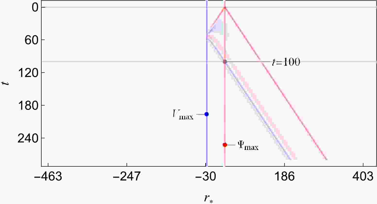
Before analyzing the influence of various parameters on QNMs, we first analyze the evolution characteristics of initial scalar perturbations in the
$ (t,r_*) $ spacetime diagram, as shown in the figure below.In this spacetime diagram of the perturbed scalar field Ψ, the chosen parameters are
$ \left\{ M \rightarrow \frac{1}{2}, a \rightarrow \frac{1}{5}, q \rightarrow \frac{1}{5}, \lambda \rightarrow \frac{1}{500}\right\}\{l \rightarrow 2\}. $

The initial perturbations are selected as
$ C_A=10; \quad C_a=1/8;\quad C_b=r_*(V_{\max})+50. $

We use this initial perturbation for all subsequent calculations.
As shown in Fig. 1, on the left side of the effective potential maximum
$V_{\max}$ , the evolution of the scalar field has only two stages: the QNM stage transmitted from the barrier, and the tail stage after some time. On the right side of the effective potential maximum$V_{\max}$ , as mentioned in the introduction, the evolution of the scalar field is divided into three stages (i.e., the initial burst, quasinormal ringing, and tail). For example, at$\Psi_{\max}$ , because the wave speed of the perturbation is 1 and$r_*(\Psi_{\max})-r_*(V_{\max})=50$ , we can infer that the arrival time of quasinormal ringing is$ t=100 $ . Hence, at$\Psi_{\max}$ , the time intervals corresponding to the three stages of scalar field evolution are shown in the figure: initial burst$ (0<t<100) $ and quasinormal ringing and tail$ (t>100) $ .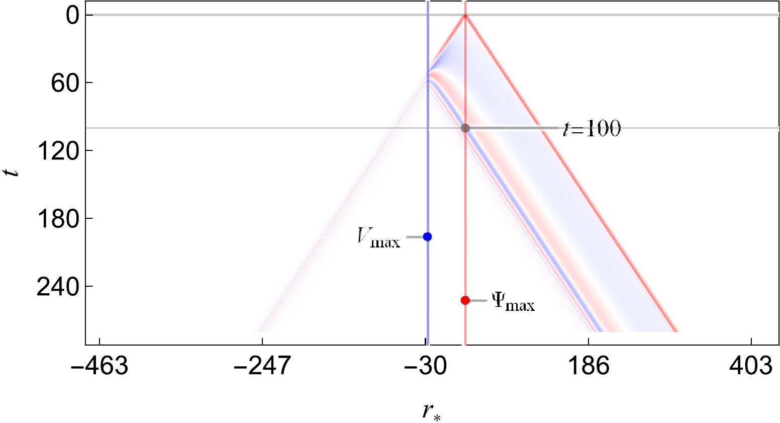
Figure 1. (color online) Evolution of the perturbed scalar field Ψ over time.
-
In this section, we analyze the influence of parameter a on QNMs. First, we fix all parameters except for a, which are set to
$ \left\{ M \rightarrow \frac{1}{2}, q \rightarrow \frac{1}{5}, \lambda \rightarrow \frac{2}{1000}\right\}\{l \rightarrow 2\}, $

while a takes four different values,
$ a= $ 0, 0.2, 0.4, and 0.6.Figure 2 shows the effective potential V outside the event horizon for different values of a.
Figure 2. (color online) Effective potential V for different values of a.
The curvature of the effective potential curve can be defined as
$ {\cal{X}}=V_2/\sqrt{(1+V_1)^3} $ in mathematics. At the peak of the effective potential, where$ V_1=0 $ ,$ {\cal{X}}_0= |V_2| $ . In general, we can directly observe the bend of the curve to compare the magnitude of$ {\cal{X}}_0 $ .We can directly see that both the peak of the effective potential and
$ {\cal{X}}_0 $ decrease as a increases.Generally, the larger the peak of the effective potential, the larger the peak of the scalar field scattered by the effective potential. In the previous analysis, it is estimated that the reflected scalar field perturbation reaches its peak at
$ t=100 $ . Figure 3 shows that at$ t=100 $ , as a increases and the peak of the effective potential gradually decreases, the peak of$ |\Psi| $ indeed decreases correspondingly.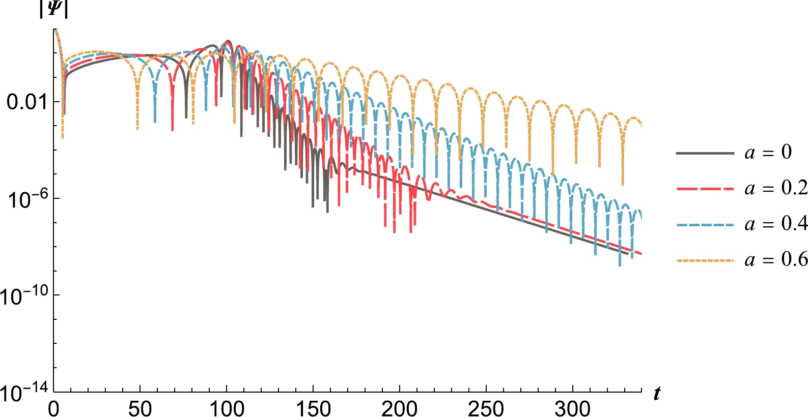
Figure 3. (color online) Evolution diagram of the scalar field perturbation Ψ for different values of a.
Similarly, the smaller the
$ {\cal{X}}_0 $ , the lower the fundamental frequency of the QNMs of the scalar field scattered by the effective potential. Figure 3 shows that as a increases and$ {\cal{X}}_0 $ at the peak of the effective potential decreases, the oscillation frequency of$ |\Psi| $ at$ t>100 $ also decreases significantly.Figure 3 shows that the string parameter a has a dramatic impact on the frequency and decay rate of the waveforms. The decay rate becomes slower as a increases.
To further verify our findings, the QNMs obtained using the WKB approximation are given in Table 1. We can see that as a increases, the real part of the fundamental frequency of the QNMs decreases, and the absolute value of the imaginary part also decreases.
This means that as a increases, the oscillation frequency in the quasinormal ringing decreases and the decay rate decreases. This is consistent with the results shown in Fig. 3. Finally, we present the corresponding greybody factors in Fig. 4. As a increases, the transmittance of the black hole horizon gradually increases, which is consistent with the decrease in the peak of the effective potential.
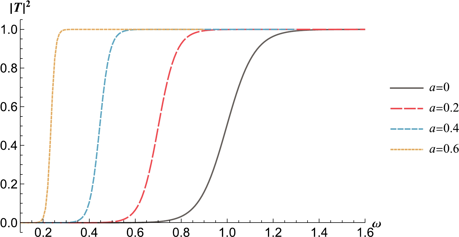
Figure 4. (color online) Greybody factor
$ |T|^2 $ for various a. -
In this section, we analyze the influence of q on QNMs. Similar to the analysis of the parameter a, we first fix all other parameters except for q as follows:
$ \left\{ M \rightarrow \frac{1}{2}, a \rightarrow \frac{1}{5}, \lambda \rightarrow \frac{2}{1000}\right\}\{l \rightarrow 2\}. $

Figure 5 shows the variation in the effective potential V for
$ q = $ 0, 0.2, and 0.4 outside the event horizon. Similarly, between the event and cosmological horizons, the effective potential is always greater than zero. The figure shows that the maximum value of the effective potential V increases with increasing magnetic charge q. However, this change is very small. The effect of q is only significant near the event horizon. When r is sufficiently large, q has a very weak effect on the effective potential V. Therefore, near the cosmological horizon, the effective potentials are almost identical in Fig. 5.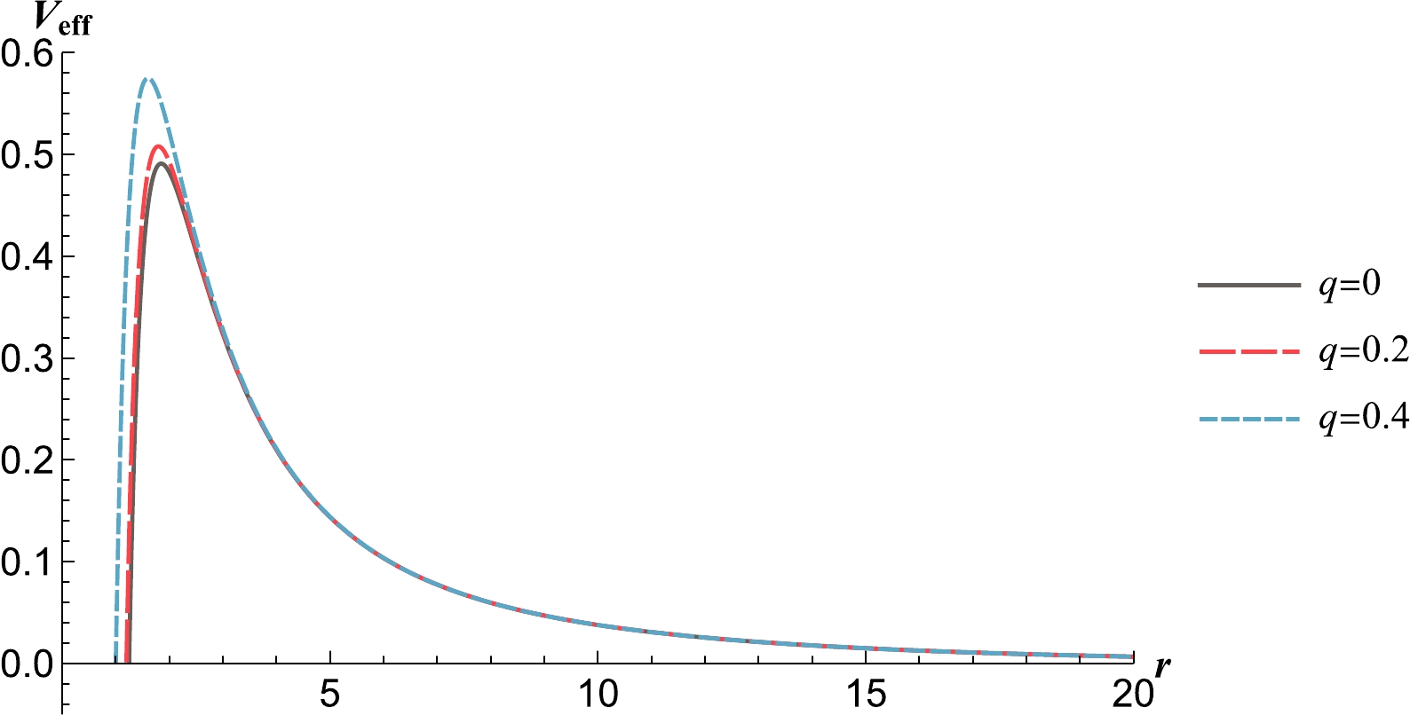
Figure 5. (color online) Effective potential V for different values of q.
The insignificant change, especially near the cosmological horizon, in the effective potential leads to an unremarkable change in the evolution of the scalar field. As shown in Fig. 6, the evolutions of the scalar field almost overlap.
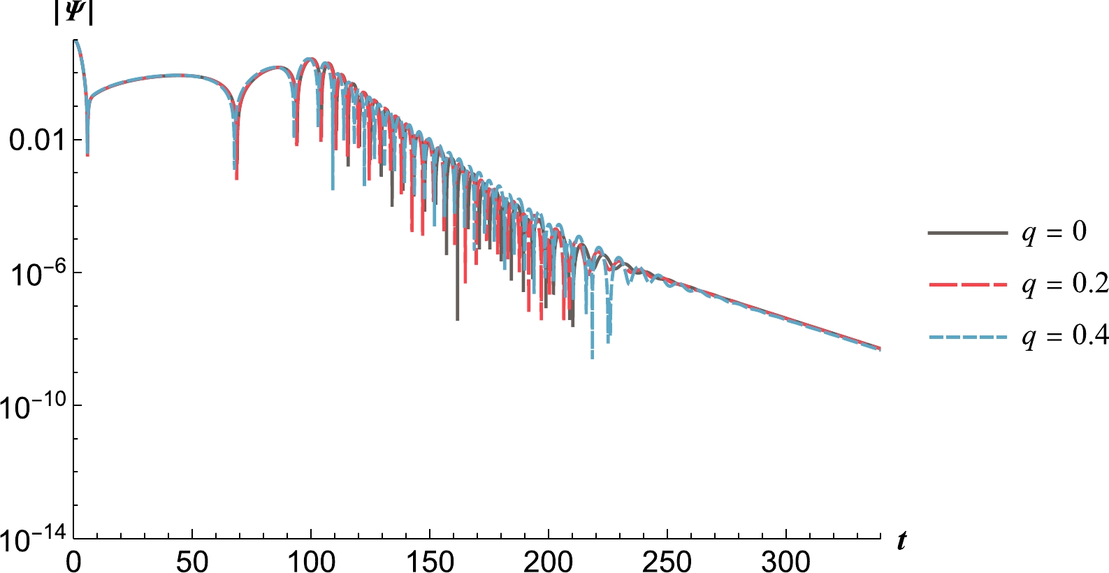
Figure 6. (color online) Evolution diagram of the scalar field perturbation Ψ for different values of q.
Similarly, we can analyze the QNMs in more detail using the WKB approximation. Table 2 shows the variation in QNMs with q. A larger q causes a higher value of the fundamental frequency
${\rm Re}(\omega)$ of QNMs, whereas the opposite trend can be observed for the value of$|{\rm Im} (\omega)|$ . This means that in quasinormal ringing, as q increases, the oscillation frequency increases, and the decay rate decreases correspondingly in Fig. 6.q n Quasinormal frequency Error estimation 0 0 0.68542516-0.12323891 i $ 3.089469 \times 10^{-7} $ 

1 0.66268336-0.37512830 i $ 6.171675 \times 10^{-7} $ 

0.2 0 0.69804982-0.12162303 i $ 3.549236 \times 10^{-7} $ 

1 0.67703312-0.36984175 i $ 9.113941 \times 10^{-6} $ 

0.4 0 0.74594502-0.11285594 i $ 5.491912 \times 10^{-7} $ 

1 0.72949588-0.34154418 i $ 8.846580 \times 10^{-6} $ 

Table 2. QNMs for different values of q in the SBBH.
Finally, in Fig. 7, we give the corresponding greybody factor, which reveals that when the frequency ω is fixed, as the parameter q increases, the greybody factor
$ |T|^2 $ decreases synchronously.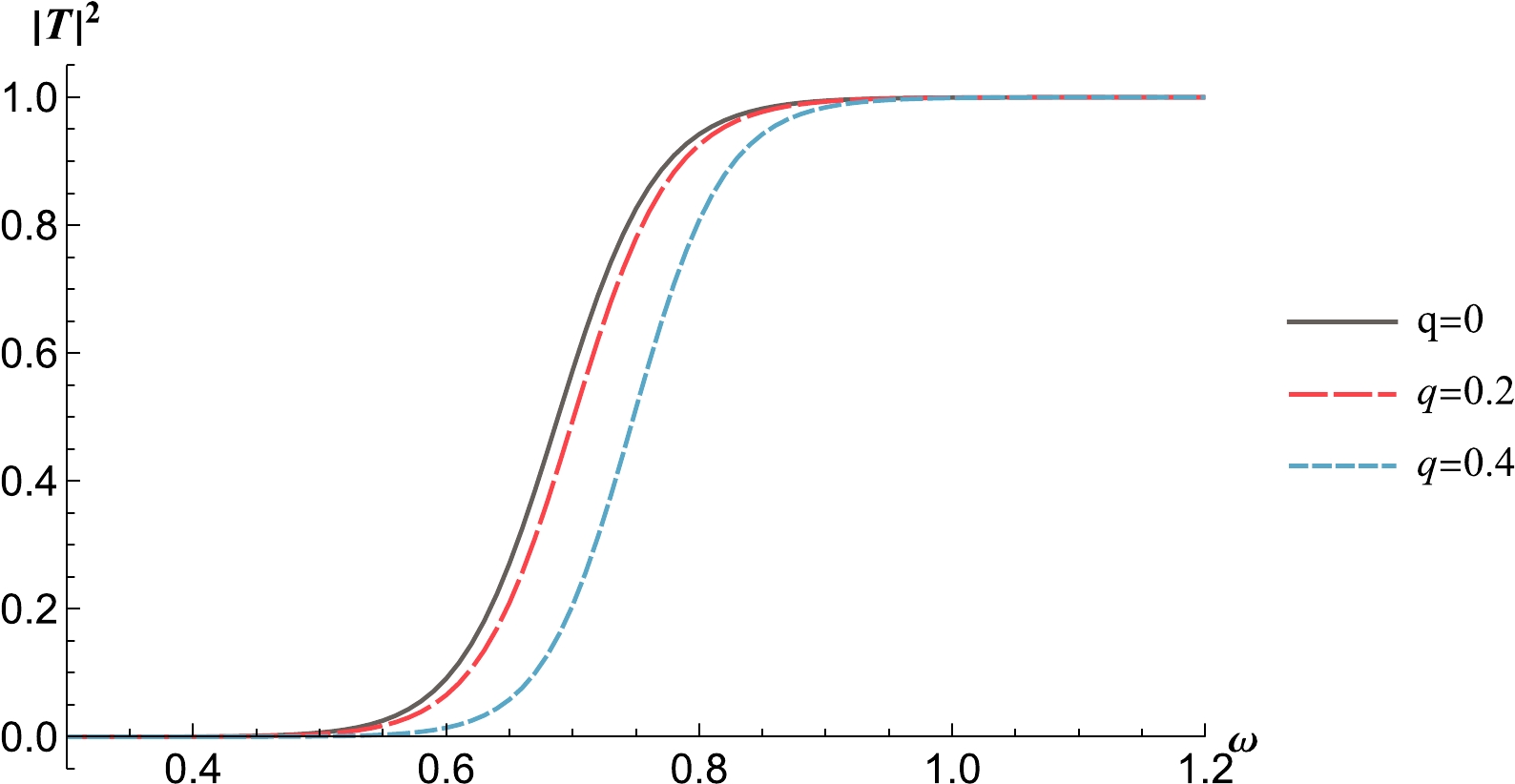
Figure 7. (color online) Greybody factor
$ |T|^2 $ for various q. -
The influence of the cosmological constant λ on QNMs is analyzed in this section. Similarly, we first determine the values of the parameters (M, a, q, l) as follows:
$ \left\{ M \rightarrow \frac{1}{2}, a \rightarrow \frac{1}{5}, q \rightarrow \frac{1}{5} \right\}\{l \rightarrow 2\}. $

In Fig. 8, we show how the effective potential V outside the event horizon changes as the parameter λ varies. We can see that as the cosmological constant λ increases, the peak value of the effective potential decreases correspondingly.
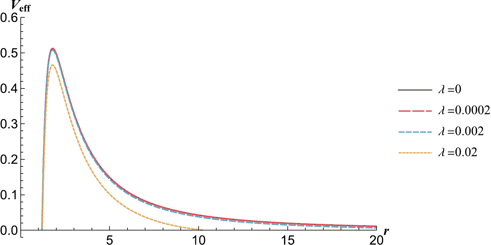
Figure 8. (color online) Effective potential V for different values of λ.
In addition, unlike q, which primarily affects the behavior of V near the event horizon, λ mainly affects V near the cosmological horizon (while at infinity for
$ \lambda=0 $ ). Meanwhile, the tail part of Ψ is mainly determined by the behavior of the effective potential near the cosmological horizon [26].As shown in Fig. 9, with the increase in the parameter λ, the tail of
$ |\Psi| $ undergoes significant changes. Compared to the almost unchanged tail caused by the parameter q, this proves the argument in [26].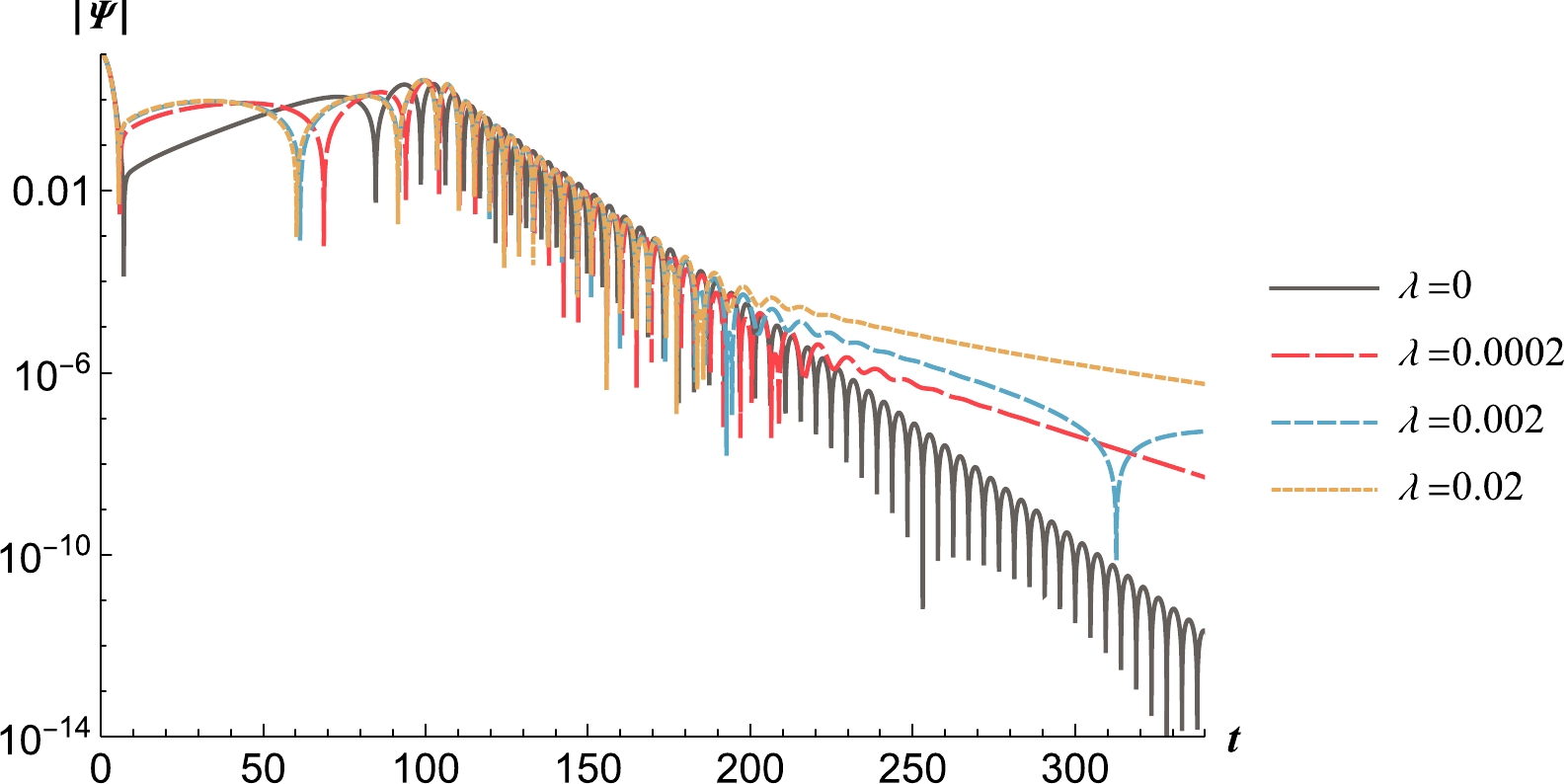
Figure 9. (color online) Evolution diagram of the scalar field perturbation Ψ for different values of λ.
Table 3 shows the QNMs obtained using the WKB approximation for different values of λ. In Table 3, the absolute values of the real and imaginary parts of the fundamental frequency of the QNMs decrease as λ increases.
λ n Quasinormal frequency Error estimation 0 0 0.70122581-0.12208316 i $ 4.601346 \times 10^{-7} $ 

1 0.67987976-0.37136248 i $ 9.182041 \times 10^{-6} $ 

0.0002 0 0.70090873-0.12203731 i $ 4.464850 \times 10^{-7} $ 

1 0.67959576-0.37121074 i $ 9.178675 \times 10^{-6} $ 

0.002 0 0.69804982-0.12162303 i $ 3.549236 \times 10^{-7} $ 

1 0.67703312-0.36984175 i $ 9.113941 \times 10^{-6} $ 

0.02 0 0.66892071-0.11731892 i $ 3.007880 \times 10^{-7} $ 

1 0.65073136-0.35581359 i $ 7.112285 \times 10^{-6} $ 

Table 3. QNMs for different values of λ in the SBBH.
Finally, in Fig. 10, the greybody factor
$ |T|^2 $ decreases as the cosmological parameter increases for a fixed frequency ω. This corresponds to the change in the peak of V with λ.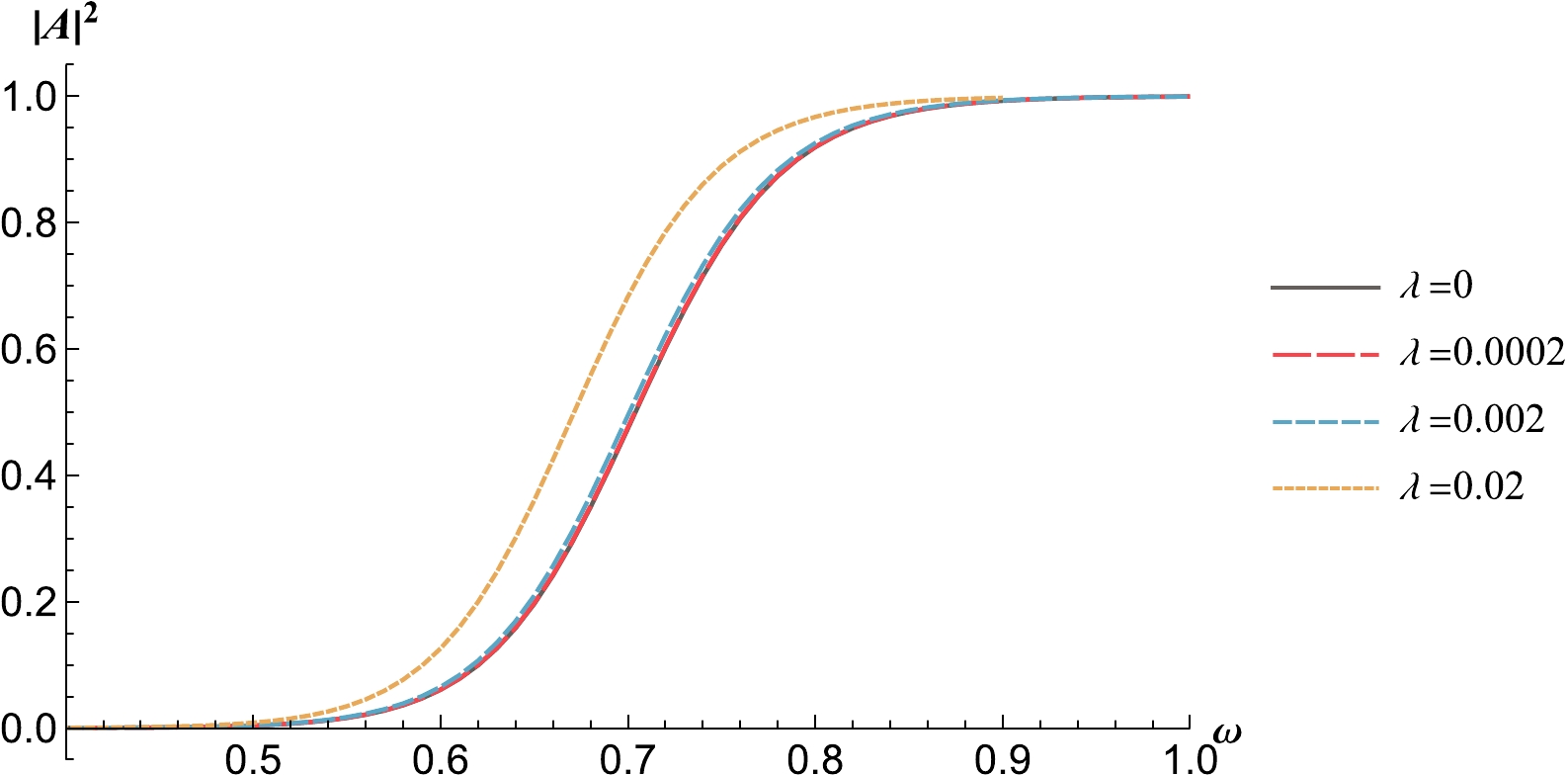
Figure 10. (color online) Greybody factor
$ |T|^2 $ for various λ. -
In this section, we analyze the influence of the parameter l on the QNMs. We first fix the parameters that are not under consideration as follows:
$ \left\{ M \rightarrow \frac{1}{2} , a \rightarrow \frac{1}{5}, q \rightarrow \frac{1}{5}, \lambda \rightarrow \frac{2}{1000}\right\}. $

In Fig. 11, we demonstrate the variation in the effective potential V outside the event horizon with respect to l. As l increases, the peak value of the effective potential increases accordingly, and
$ {\cal{X}}_0 $ also increases. This behavior is similar to that of a. Correspondingly, during the quasinormal ringing phase$ 100<t<t_t $ (where$ t_t $ denotes the start of the tail phase) shown in Fig. 12, we observe that the oscillation frequency of Ψ increases with l, and the amplitude of Ψ slightly increases around$ t=100 $ with increasing l.
Figure 11. (color online) Effective potential V for
$ l=0, 1, 2, 3 $ .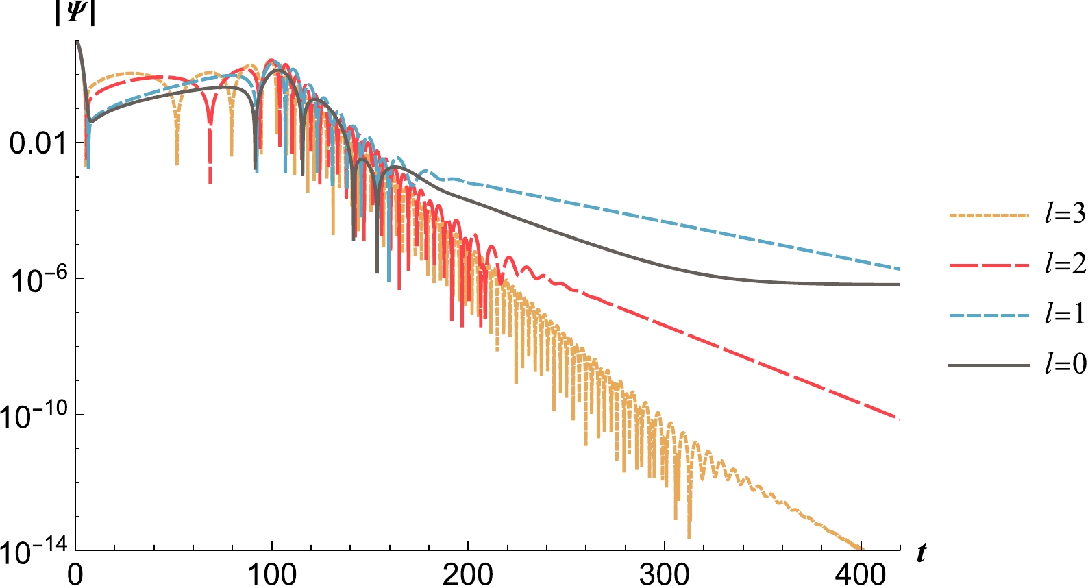
Figure 12. (color online) Evolution diagram of the scalar field perturbation Ψ for
$ l=0, 1, 2, 3 $ .Interestingly,on the black solid line in Fig. 12, when
$ l=0 $ , a nearly flat tail appears around$ t\approx 320 $ , which corresponds to the de Sitter phase, as described in Refs. [29, 42, 43].It is worth noting that when
$ l>0 $ , the effective potential remains greater than zero between the event horizon and the cosmological horizon. However, when$ l=0 $ , the effective potential no longer represents a mere potential barrier but rather a potential well. For example,$V_{\rm eff}(20)= -0.000584$ . This implies that the physical system may harbor bound states.Next, we present detailed results on the QNMs obtained using the WKB approximation in Table 4 for
$ l=0, 1, 2, 3 $ . From Table 4, we observe that as l increases, the real part of the fundamental frequency of QNMs gradually increases, whereas the absolute value of the imaginary part decreases. Thus, during the quasinormal ringing phase, the oscillation frequency increases and the decay rate decreases with increasing l, as shown in Fig. 12.In Fig. 13, we plot the greybody factor
$ |T|^2 $ for various l. The decrease in the greybody factor with increasing l correlates with the increase in the peak value of the effective potential.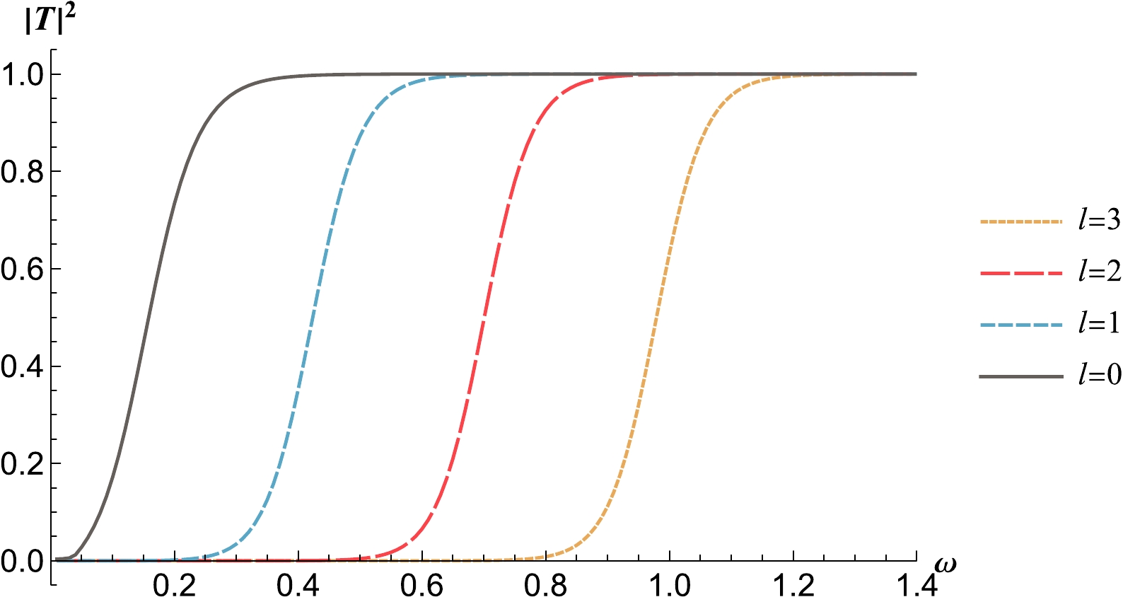
Figure 13. (color online) Greybody factor
$ |T|^2 $ for various l. -
Finally, we use the Prony method [41] to further confirm the connection between our numerical calculations and the WKB approximation. In this section, the parameters are chosen as
$ \left\{ M \rightarrow \frac{1}{2} , a \rightarrow \frac{1}{5}, q \rightarrow \frac{1}{5}, \lambda \rightarrow \frac{2}{1000}\right\}\{l \rightarrow 2\}. $

We extract the data at
$V_{\max}$ in the interval$ 100<t< 150 $ , as shown in Fig. 14, and obtain the real and imaginary parts of the corresponding QNMs through the Prony method:$\omega_{\rm Prony}=0.698097-0.121650{\rm{i}}$ . Correspondingly, the result obtained through the WKB approximation is$\omega_{\rm WKB}=0.6980498152-0.1216230302{\rm{i}}$ .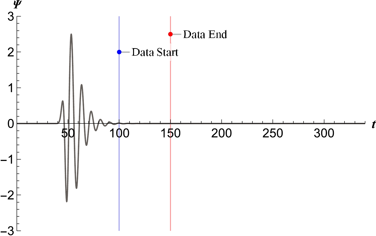
Figure 14. (color online) Time domain solution of Ψ over time at
$V_{\max}$ .Combined with Eq. (16), the fitting function can be written as
$ \Psi_{\rm Prony} = C_a \exp(-0.121650 t) \sin(0.698097 t + C_o), $

(22) where
$ C_a = 2344.25 $ and$ C_o = -2.16557 $ . In Fig. 15, the red dashed line is the fitted curve of Eq. (22), and the black solid line is the data obtained using the numerical method.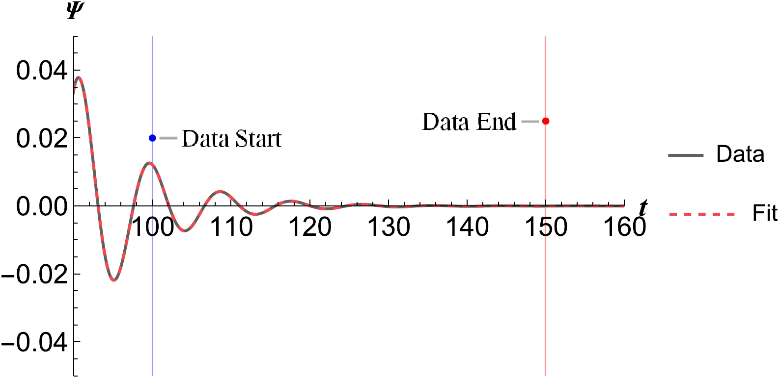
Figure 15. (color online) Fitted graph of the evolution of Ψ.
Finally, we can use the following error estimate method:
$ \delta=\frac{\left|\omega_{\rm WKB}-\omega_{\rm Prony}\right|}{\left|\omega_{\rm WKB}\right|}.$

(23) We obtain the corresponding error as
$ \delta=7.67\times 10^{-5} $ . This result, in turn, ensures the accuracy of our numerical calculations. -
In this paper, we investigate scalar perturbations in the SBBH using the FEM and WKB approximation, unlike in [15], We directly use the integral method to deal with the problem of the turtle coordinates having no analytic solution in Bardeen space-time. Then, using the numerical method, we obtain the slices of time evolution corresponding to QNMs of the scalar perturbation. We also calculate the corresponding QNMs and greybody factors using the WKB approximation. The results of the WKB scheme, the time domain diagram of the perturbation evolution, and the effective potential are all related. Finally, we further verify the accuracy of our calculations through the Prony method.
The conclusions can be summarized as follows:
1. In the time domain, the evolution of a scalar field does not increase with time. Correspondingly, in the WKB approximation, the imaginary part of the QNM frequency is always negative. This implies that the space-time under scalar perturbations is stable.
2. As the parameter a increases, the QNM frequency and decay rate decrease. This is because a larger parameter a results in a smoother effective potential with lower peaks owing to the presence of string clouds weakening the effect of the original Bardeen background spacetime, which makes it flatter.
3. Simultaneously, with an increase in the parameter a, the greybody factor also increases proportionally. The presence of string clouds weakens the relative change in the effective potential, resulting in lower peak values and facilitating scalar field penetration through the potential barrier, thereby increasing the greybody factor.
4. Conversely, an increase in the parameter q leads to an increase in QNM frequency, a slight reduction in decay rate, and a smaller greybody factor. It has almost no effect on the tail because q only affects the effective potential near the event horizon and can be ignored near the cosmological horizon.
5. Increasing the cosmological constant λ from zero results in a slight decrease in both the QNM frequency and decay rate. However, there is a significant modification in the tail behavior, which is consistent with the notable impact of the cosmological constant λ at large
$ r_* $ values.6. With an increase in angular quantum number l, the QNM frequency increases, whereas the decay rate slightly decreases. Additionally, the greybody factor decreases correspondingly.
It is worth noting that when
$ l=0 $ , a de Sitter phase occurs at$ t\approx 320 $ [29]. We posit that this occurrence relates to the negative potential well that appears at$ l=0 $ . At this point, bound states may exist, which produce a residual scalar field$ \Psi_0 $ in the tail. A simple analysis is available in Appendix B.This study only investigated scalar perturbations in SBBH spacetime. It will be interesting and straightforward to extend this work to vector and gravitational perturbations, especially for QNMs under gravitational perturbations, which reflect the fundamental characteristics of gravitational waves during the ringdown stage. These topics merit further exploration in the future.
-
First, before numerical computation of turtle coordinates, we can divide the background spacetime into two categories and discuss them separately.
The first category is when the cosmological constant
$ \lambda=0 $ . In this case, only the event horizon$ r_h $ exists in the background spacetime, and there is no cosmological horizon. This means that when$ r\rightarrow r_h $ ,$ r_{*}\rightarrow -\infty $ and when$ r\rightarrow +\infty $ ,$ r_{*}\rightarrow +\infty $ .The second category is when the cosmological constant
$ \lambda \neq 0 $ . In this case, both the event horizon$ r_h $ and cosmological horizon$ r_c $ exist in the background spacetime. This means that when$ r\rightarrow r_h $ ,$ r_{*}\rightarrow -\infty $ and when$ r\rightarrow r_c $ ,$ r_{*}\rightarrow +\infty $ .From the definition of turtle coordinates, we can obtain the integral function of
$ r_{*}(r) $ :$ r_{*}(r) = \int_{r_0}^{r} \frac{1}{f(\bar{r})} {\rm d}\bar{r}, \tag{A1} $

where
$ r_0 $ is an artificial selected integration parameter. In our calculation, when$ \lambda=0 $ , we choose$ r_0=2 r_h $ . When$ \lambda \neq 0 $ , we choose$ r_0=(r_h + r_c)/2 $ . Note that the different choices of$ r_0 $ only cause a change in the integration constant$ C_0 $ and do not change the definition of the turtle coordinates.In the integration, we encounter two problems. First, the integral Eq. (A1) is a singular integral, and when
$ r_{*}(r) $ is close to the event and cosmological horizons, it can usually be approximated by a logarithmic relationship:$r_* = C_h {\rm Log}(r-r_h)+C_{h0}$ when$ r\rightarrow r_h $ ;$r_* = - C_c {\rm Log}(r_c-r)+C_{c0}$ when$ r\rightarrow r_c $ .For example, if we need to compute the integral to
$ r_*(r)=-800 $ , let$ r=r_h+\epsilon $ , and we can obtain$ \begin{aligned}[b] -800 =& C_h \ln(r_h+\epsilon-C_{h0})+C_h \\ =& C_1 \ln(\epsilon)+C_{h0}\Leftrightarrow \epsilon={\rm e}^{{-(800+C_{h0})}/{C_h}}. \end{aligned}\tag{A2} $

When the spacetime background parameters are selected as
$ a=1/5,M_1=0,M=1/2,q=2/5,\lambda=1/50 $ , we obtain the fitting parameters$ C_h=2.202 $ and$ C_{h0}=-3.710 $ . At this point, the working accuracy requirement reaches${\rm e}^{{-(800-3.710)}/{2.202}}={\rm e}^{-361.621} \sim 10^{-158}$ . The numerical integration precision requirement for Eq. (A1) is very high. Therefore, we must pay attention to ensuring the working precision is sufficiently large. At the same time, if the working precision is too high, it will lead to a sharp increase in computing resources. Therefore, we must choose an appropriate working precision for numerical integration according to the calculation demand.In addition, we only use the relationship between
$ r_* $ and r in the time evolution equation. Furthermore, we usually require$ r_* $ to be selected as a series of equidistant points. Obtaining the corresponding r values for this series of equidistant turtle coordinates is not easy. Generally, we know the analytical relationship between$ r_* $ and r and then obtain the r values corresponding to a series of equidistant turtle coordinates.In this paper, because the analytical solution is unknown, and the working accuracy requirement is very high, the computational cost is substantial. Therefore, we adopt an interpolation method to obtain the r values corresponding to a series of equidistant turtle coordinate points. The steps are as follows:
1. Select a series of appropriate r values and integrate to obtain the corresponding
$ r_* $ values. For example, when the cosmological constant is non-zero, we divide the r series values into two segments:$ (r_h+\epsilon_h,r_0) $ and$ (r_0,r_c-\epsilon_c) $ . In the segment$ (r_h+\epsilon_h,r_0) $ , we choose the r series values as$ r_h+\epsilon_h+(r_0-r_h-\epsilon_h)/\epsilon_h^{(m-k)/m} $ . In the segment$ (r_0,r_c-\epsilon_c) $ , we choose the r series values as$ r_c-\epsilon_c+(r_c-r_0-\epsilon_c)/\epsilon_c^{(m-k-1)/m} $ . Here, n is the number of points, and$ k=1,2,...,m $ is the series value.2. Perform integration for each r value to obtain the corresponding
$ r_* $ .3. Select a series of equidistant
$ r_* $ values within the range of the integrated$ r_* $ values and use interpolation to obtain the corresponding r values.When m is sufficiently large, the error caused by interpolation becomes small enough to be negligible. Here, for different background spacetime parameters, we choose the appropriate parameters
$ +\epsilon_h $ and$ \epsilon_c $ such that$ r_h+\epsilon_h $ and$ r_c-\epsilon_c $ correspond to$r_{*\min}\sim -800$ and$r_{*\max}\sim 800$ and set$ m=40000 $ . -
We assume that after a substantial period of time, the evolution of the scalar field reaches a steady state, where Ψ is fixed at constant values. This implies that Ψ no longer varies with time, i.e.,
$ \Psi_{j}^{k+1}=\Psi_{j}^{k}=\Psi_{j} $ . Under this assumption, the difference Eq. (13) simplifies to$ \begin{aligned}[b] \Psi_{j}=& -\Psi_{j} +\left(2-2 \frac{\Delta t^{2}}{\Delta r_{*}^{2}}-\Delta t^{2} V_{j}\right) \Psi_{j} \\ & +\frac{\Delta t^{2}}{\Delta r_{*}^{2}}\left(\Psi_{j-1}+\Psi_{j+1}\right) . \end{aligned}\tag{B1} $

Further simplification yields the expression
$ \Psi_{j} = \frac{1}{\left(2 +\Delta r_{*}^{2} V_{j}\right)}\left(\Psi_{j-1}+\Psi_{j+1}\right). \tag{B2}$

When
$V_{\rm eff}$ is always greater than zero,$ \Psi_{j} <\left(\Psi_{j-1}+ \Psi_{j+1}\right)/2 $ forms a concave function. As$ j\rightarrow \infty $ ,$ \Psi_{j}\rightarrow \infty $ , leading to instability. Therefore, if there is a constant non-zero residual$ \Psi_0 $ [42, 43], the effective potential must have negative values (i.e., a potential well).
Quasinormal modes of Bardeen black holes with a cloud of strings
- Received Date: 2023-07-27
- Available Online: 2023-12-15
Abstract: We investigate the quasinormal mode and greybody factor of Bardeen black holes with a cloud of strings via the WKB approximation and verify them using the Prony algorithm. We find that the imaginary part of the quasinormal mode spectra is always negative, and the perturbation does not increase with time, indicating that the system is stable under scalar field perturbation. Moreover, the string parameter a has a dramatic impact on the frequency and decay rate of the waveforms. In addition, the greybody factor increases when a and λ increase and when q and l decrease. The parameters λ and l have a significant effect on the tails. In particular, when


 DownLoad: