


 Abstract
 HTML
HTML Reference
 Related
 PDF
PDF


-
Fission fragment mass and charge yields have a wide range of applications in various fields, ranging from understanding the r-process of nucleosynthesis in astrophysical physics to reactor operations. However, fission is a complicated dynamical process of quantum many body systems, and for such a large-scale collective motion and production of hundreds of isotopes characterized by different charge and mass yields and kinetic energies [1−5], many challenges regarding its mechanism are yet to be fully understood [5−10].
The experimental distributions of fission yields are rather complex. The yield distribution of nuclear fission has been observed to have the structure of single, double, and triple peaks [5, 11−14]. Inspired by the abundant experimental data, many approaches have been developed to analyze the observed data and understand the fission mechanism [15−24]. There are two main methods of calculating the fission yield distribution: the dynamical approach [25−29] and statistical approach [30−33]. These two approaches require the potential energy surface as the input.
The macroscopic-microscopic model [3, 4, 24, 34] and microscopic model [13, 35] have been widely used to calculate the potential energy surface of the fission process. However, the calculation of the multidimensional potential energy surface for a heavy nuclear system is a complicated physical problem that has not yet been fully solved because choosing the appropriate common degrees of freedom is an important and difficult task. The number of degrees of freedom should not be too large to allow for the numerical analysis of the corresponding dynamical equations. Therefore, the calculated potential energy surface is the upper limit of the optimum potential that the nucleus can adopt [24].
It is important to note the strong dependence of microscopic effects on the temperature (or excitation energy) of the nucleus. At higher energies, temperature effects should be included not only in the potential energy surface [36−40] but also in the friction and mass tensors in the dynamical equations. However, this is rarely done. In addition, to describe the yields of a compound nucleus at higher excitation energies, it is necessary to consider multi-chance fission [41]. However, estimating the percentages of multi-chance fission contributions is difficult and has considerable uncertainties [41, 42]. Therefore, it is both experimentally and theoretically challenging to obtain accurate and complete energy dependent distributions of fission yields for any fissile nucleus (
$ ^{A}_{Z}X $ ).An alternative class of approaches being actively explored is based on machine learning techniques. Although machine learning methods have been increasingly applied to the many body problem in condensed matter, quantum chemistry, and quantum information over the past few years, there are significantly more machine learning applications in low-energy nuclear physics, such as neutron induced fission yield distributions [43−48], nuclear masses [49−51], and various nuclear reactions and structural properties [52−57]. The main objective of this study is to evaluate energy dependent neutron induced fission yields based on the Bayesian neural network (BNN) approach.
-
The principle of Bayes' rule is to establish a posterior distribution from all unknown parameters trained by a given data sample [58]. A detailed description of the origins and development of BNNs goes beyond the scope of this study; hence, we limit ourselves to highlighting the main features of the approach.
The BNN approach to statistical inference is based on Bayes's theorem, which provides a connection between a given hypothesis (in terms of problem-specific beliefs for a set of parameters ω) and a set of data
$ (x,t) $ to a posterior probability$ p(\omega\mid x,t) $ that is used to make predictions on new inputs. In this context, Bayes's theorem may be written as [59]$ \begin{equation} p(\omega\mid x,t)=\frac{p(x,t\mid\omega) p(\omega)}{p(x,t)}, \end{equation} $

(1) where p(ω) is the prior distribution of the model parameters ω, and
$ p(x,t\mid \omega) $ is the “likelihood” that a given model ω describes the new evidence$ t(x) $ . The product of the prior and likelihood form the posterior distribution$ p(\omega \mid x,t) $ , which encodes the probability that a given model describes the data$ t(x) $ .$ p(x,t) $ is a normalization factor, which ensures that the integral of the posterior distribution is 1. In essence, the posterior represents the improvement to$ p(\omega) $ as a result of the new evidence$ p(x,t\mid \omega) $ .In this study, the inputs of the network are given by
$ x_{i}= \{Z_{i},N_{i},A_{i},E_{i}\} $ , which includes$ Z_{i} $ (the number of charges of the fission nucleus),$ N_{i} $ (the number of neutrons in the fission nucleus),$ A_{i} $ (the mass number of fission fragments), and$ E_{i}=e_{i}+S_{i} $ (neutron incident energy plus neutron separation energy).The neural network function
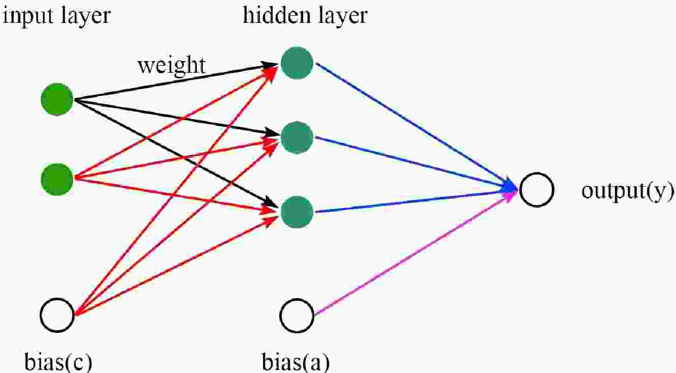
$ f(x,\omega) $ adopted here has the following “sigmoid” form [60−62]:$ \begin{equation} f(x,\omega)=a+\sum\limits_{j=1}^{H} b_{j} \tanh \left(c_{j}+\sum\limits_{i=1}^{l} d_{i j} x_{i}\right), \end{equation} $

(2) where the model parameters are collectively given by
$ \omega=\{a,b_{j},c_{j},d_{ij}\} $ . H is the number of neurons in the hidden layer, I is the number of inputs, a is the bias of the output layers,$ b_{j } $ is the weights of output layers,$ c_{j} $ is the bias of the hidden layers, and$ d_{j i} $ is the weights of the hidden layers. The tanh is a common form of the sigmoid activation function that controls the firing of artificial neurons. A schematic diagram of a neural network with a single hidden layer, three hidden neurons$(H=3) $ , and two input variables$(I=2) $ is shown in Fig. 1.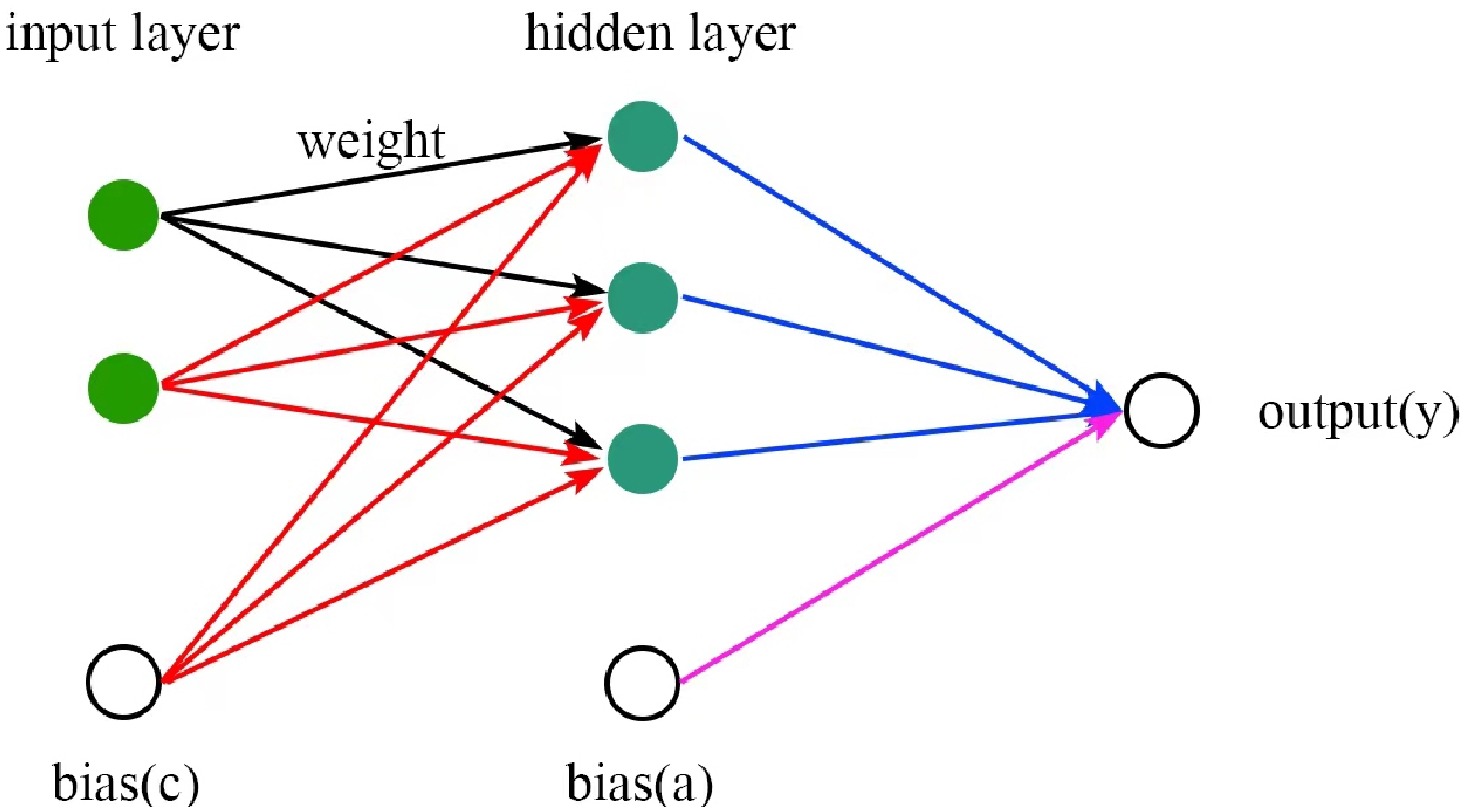
Figure 1. (color online) Schematic diagram of a neural network with a single hidden layer, three hidden neurons (H = 3), and two input variables (I = 2).
To determine the optimal number of hidden layers and neurons in a neural network, we employ the technique of cross-validation. First, we estimate a rough range for the model based on prior research papers. Subsequently, we randomly partition our dataset into two parts, one for training and the other for testing. We repeat this process, swapping the roles of the training and testing sets each time. We then compute the average prediction errors obtained from training the model twice with each set to estimate the performance of our BNN model. Based on our analysis, we determine that the optimal configuration has double hidden layers, each consisting of 16 neurons.
Bayesian inference for neural networks calculates the posterior distribution of the weights given the training data,
$ p(\omega\mid x,t) $ . This distribution answers predictive queries about unseen data using expectations. Each possible configuration of the weights, weighted according to the posterior distribution, makes a prediction about the unknown label given the test data item x [63].In this study, we adopt a variational approximation to the Bayesian posterior distribution on the weights. To obtain an estimate of the maximum a posteriori of ω, we use variational learning to find a probability
$ {q}\left(\omega \mid \theta_{\omega }\right) $ to approximate the posterior probability of ω. To do this, we use Kullback-Leibler divergence to minimize the distance between the probabilities$ {q}\left(\omega \mid \theta_{\omega }\right) $ and$ {p}(\omega \mid \mathrm{\mathit{x,t} }) $ [64−67],$ \begin{aligned} \theta^{*} &=\arg \min _{\theta_{\omega }} \mathrm{KL}\left[ {q}\left(\omega \mid \theta_{\omega}\right) \| {p}(\omega \mid {\mathit{x,t} })\right] \\ &=\arg \min _{\theta_{\omega}} \int {q}\left(\omega \mid \theta_{\omega}\right) \ln \frac{ {q}\left(\omega \mid \theta_{\omega}\right)}{ {p}( {\mathit{x,t} } \mid \omega) {p}(\omega)} \mathrm{d} \omega \\ &=\arg \min _{\theta_{\omega}} \mathrm{KL}\left[ {q}\left(\omega \mid \theta_{\omega}\right) \| {p}(\omega)\right]- {E}_{ {q}\left(\omega \mid \theta_{\omega}\right)}[\ln {p}( {\mathit{x,t} } \mid \omega)]. \end{aligned} $

Then, the loss function of the BNN can be written in the following form:
$ \mathrm{F}\left( {\mathit{x,t} }, \theta_{\omega }\right)=\mathrm{KL}\left[ {q}\left(\omega \mid \theta_{\omega }\right) \| {p}(\omega )\right]- {E}_{ {q}\left(\omega \mid \theta_{\omega }\right)}[\ln {p}( {\mathit{x,t} } \mid \omega )]. $

Finally, using the Monte Carlo method, we can obtain an approximate result.
-
In the process of running the program, we find that the function is often trapped in a local minimum point. Therefore, the results obtained by each program are always different. In particular, when there is no experimental data for extrapolation, we have no way of judging which results are correct. Therefore, we use a method similar to the annealing evolution algorithm. At each iteration, the program has a certain probability of accepting a solution that is worse than the current one; hence, it is likely to jump out of the local optimal solution and reach the global optimal solution. After adding this mechanism, the effect is significant, and the difference between the results after each program execution is within an acceptable range.
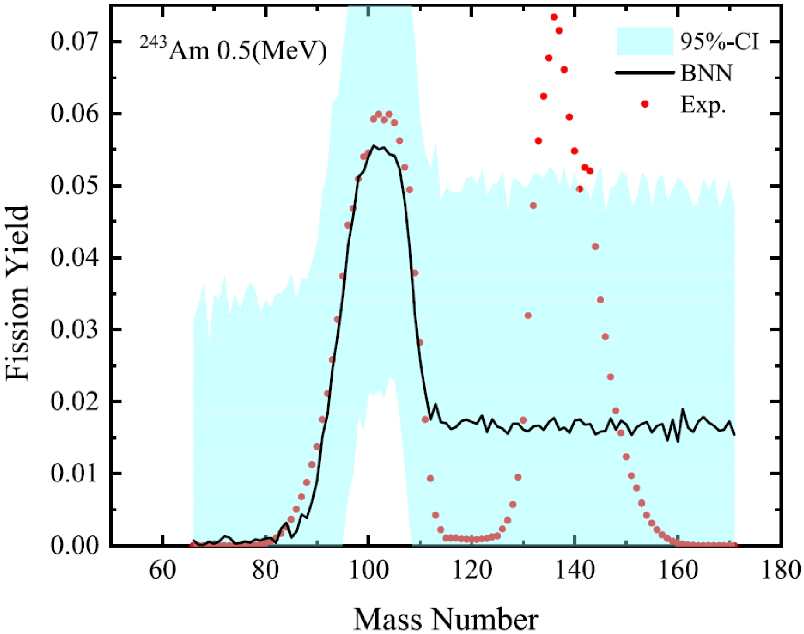
In the absence of simulated annealing, iterative processes may lead to outcomes characterized by local optima, as shown in Fig. 2. This occurrence can be attributed to the iterative nature of the algorithm becoming trapped in suboptimal solutions. Conversely, the utilization of simulated annealing in neural networks mitigates this concern by effectively navigating the search space and avoiding convergence to suboptimal solutions.
To test the performance of the BNN approach, the independent mass distributions of the neutron induced fission of n+
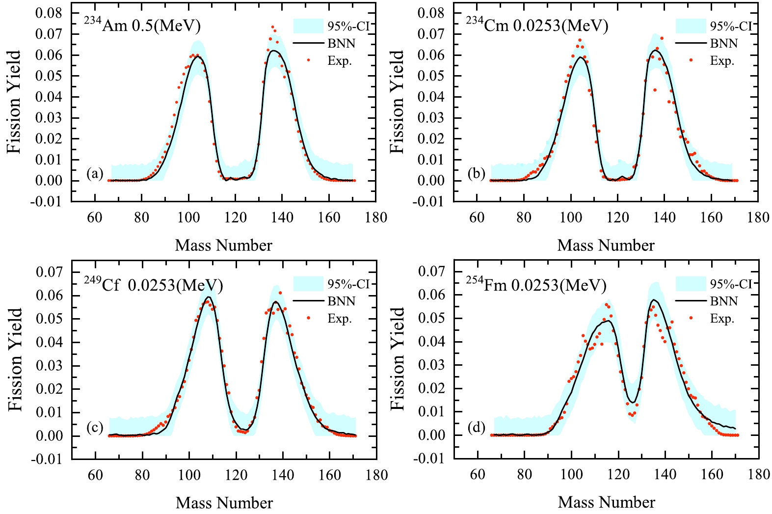
$ ^{A}_{Z}X $ with a neutron incident energy are studied. The training dataset$ ^{227} $ Th(0.0253),$ ^{229} $ Th(0.0253),$ ^{232} $ Th(0.5),$ ^{232} $ Th(14),$ ^{232} $ Th(22.5),$ ^{231} $ Pa(0.5),$ ^{232} $ U(0.0253),$ ^{233} $ U(0.0253),$ ^{233} $ U(0.5),$ ^{233} $ U(14),$ ^{234} $ U(0.5),$ ^{234} $ U(14),$ ^{235} $ U(0.0253),$ ^{235} $ U(0.5),$ ^{235} $ U(5.04),$ ^{235} $ U(14),$ ^{235} $ U(15.5),$ ^{236} $ U(0.5),$ ^{236} $ U(14),$ ^{236} $ U(20),$ ^{237} $ U(0.5),$ ^{238} $ U(0.5),$ ^{238} $ U(1.6),$ ^{238} $ U(2),$ ^{238} $ U(3),$ ^{238} $ U(4.5),$ ^{238} $ U(5.5),$ ^{238} $ U(5.8),$ ^{238} $ U(10),$ ^{238} $ U(10.05),$ ^{238} $ U(13),$ ^{238} $ U(14),$ ^{238} $ U(16.5),$ ^{238} $ U(20),$ ^{238} $ U(22.5),$ ^{237} $ Np(0.0253),$ ^{237} $ Np(0.5),$ ^{237} $ Np(1),$ ^{237} $ Np(2),$ ^{237} $ Np(4),$ ^{237} $ Np(5.5),$ ^{237} $ Np(14),$ ^{238} $ Np(0.5),$ ^{238} $ Pu(0.5),$ ^{240} $ Pu(0.0253),$ ^{240} $ Pu(0.5),$ ^{232} $ Pu(14),$ ^{241} $ Pu(0.0253),$ ^{241} $ Pu(0.5),$ ^{242} $ Pu(0.0253),$ ^{242} $ Pu(0.5),$ ^{242} $ Pu(14),$ ^{241} $ Am(0.0253),$ ^{241} $ Am(0.5),$ ^{243} $ Am(0.5),$ ^{242} $ Cm(0.5),$ ^{243} $ Cm(0.0253),$ ^{243} $ Cm(0.5),$ ^{244} $ Cm(0.5),$ ^{245} $ Cm(0.0253),$ ^{246} $ Cm(0.5),$ ^{248} $ Cm(0.5),$ ^{251} $ Cf(0.0253),$ ^{254} $ Es(0.0253),$ ^{254} $ Fm(0.0253),$ ^{255} $ Fm(0.0253) is taken from Refs. [24, 68−70]. The neutron energy is in parentheses.We apply the BNN to learn the existing evaluated distributions of mass yields, which includes 6996 data points of the neutron induced fissions of 66 nuclei. To examine the validity of the BNN approach, we separate the entire dataset into learning and validation sets with a combination of 65+1. The learning set is constructed by randomly selecting 65 nuclei from the entire set, and the remaining 1 nucleus composes the validation set. The evaluation results of the randomly selected validation set (eight nuclei) are shown in Figs. 3 and 4. As shown in Figs. 3 and 4, the evaluation of the BNN is satisfactory, and the distribution positions can be well described using the BNN approach. Note that the evaluation is less satisfactory around
$ ^{254} $ Fm, where neighboring nuclei in the learning set are not sufficient. This indicates that the BNN approach is effective for existing evaluated distributions of mass yields, and there is no overfitting, even with only the learning set data.
Next, we analyze the results with the data of
$ ^{255} $ Fm(0.0253) excluded in the learning set. In this case, with 6890 points, the total$ \chi^{2}_{N}=\sum _{i}[t_{i}- f(x_{i})]^{2}/N $ is$ 2.24\times10^{-5} $ . Figures 5 and 6 show the calculated results of the mass distributions of$ ^{238} $ U(n, f) at different neutron energies, which are compared with experimental data. We can see that the training results are in good agreement with experimental data in the neutron energy range from 0.50 to 22.50 MeV; the peak-to-valley ratio decreases with increasing energy. The BNN can remarkably reproduce the overall evaluated fission yields.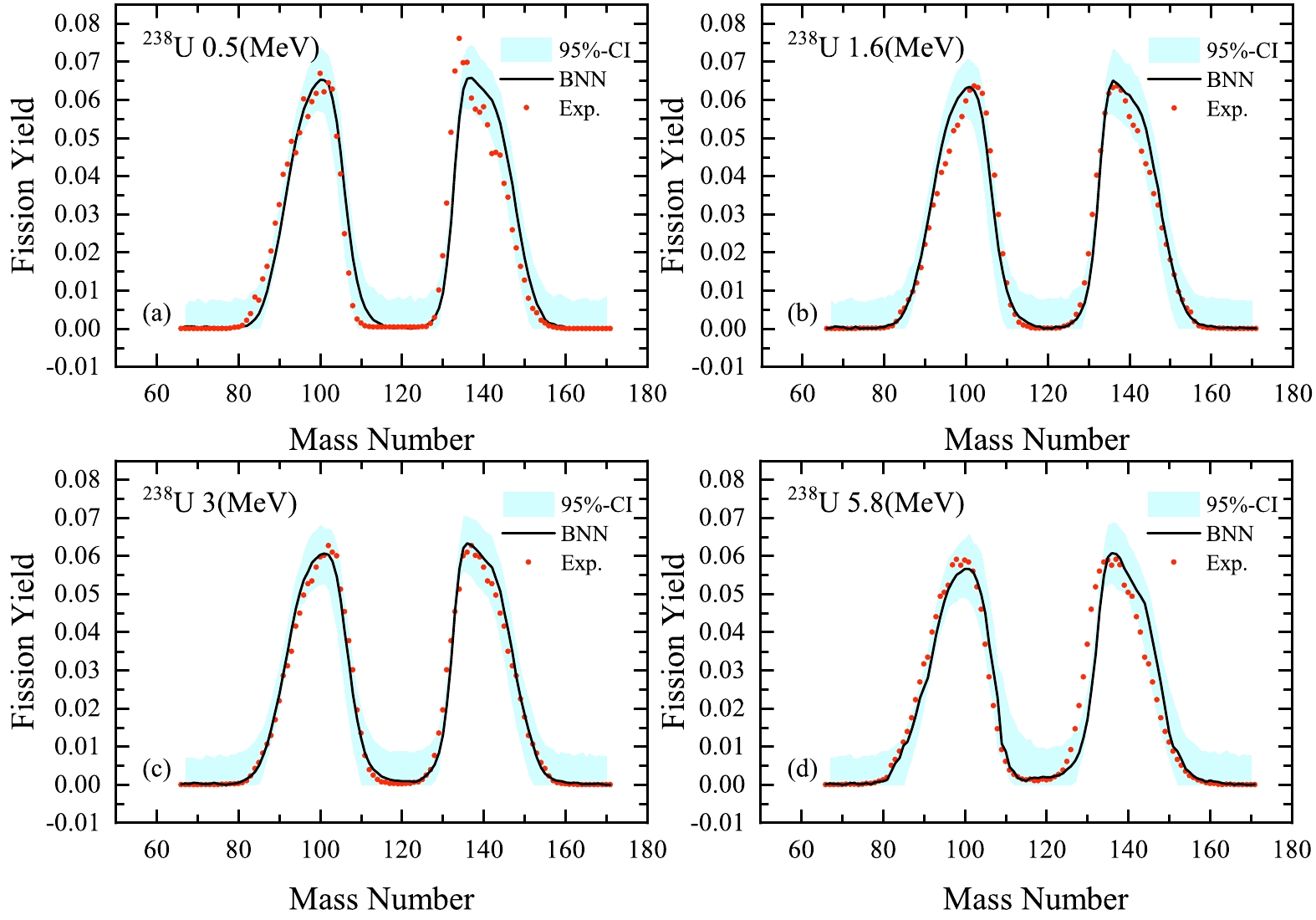

To study the influence of excitation energy on the shape of the mass distribution, we calculate
$ ^{238} $ U at incident neutron energies of 1.6, 5.8, 16.5, and 22.5 MeV, as shown in Fig. 7. There are obvious changes such as the increase in valley height and the decrease in peak height in the mass distributions with increasing incident neutron energy. It is known that the symmetric fission mode plays a role as excitation energies increase. Our training results demonstrate that the features of energy-dependent fission yields can be successfully described by the BNN evaluation.
Figure 7. (color online) Calculated mass distributions for the
$^{238}$ U(n, f) reaction at different incident-neutron-energies.The main motivation of our BNN approach is to estimate incomplete experimental distributions of fission yields based on the information learned from completed evaluations of other nuclei. It is well known that only a few experimental data points are available for some nuclei. Figure 8(a)−(c) show the calculated results using the BNN for the fission yields of n+
$ ^{238} $ U at energies of 3.60, 4.49, and 14.8 MeV. The calculated mass distributions of the fragments are denoted by solid lines. From a comparison of the experimental data with the results evaluated using the BNN, taking into account the experimental data, we find that the BNN predictions without learning the experimental data are satisfactory. Our BNN method is found to be reliable in predicting the fission fragment mass distributions for interpolation.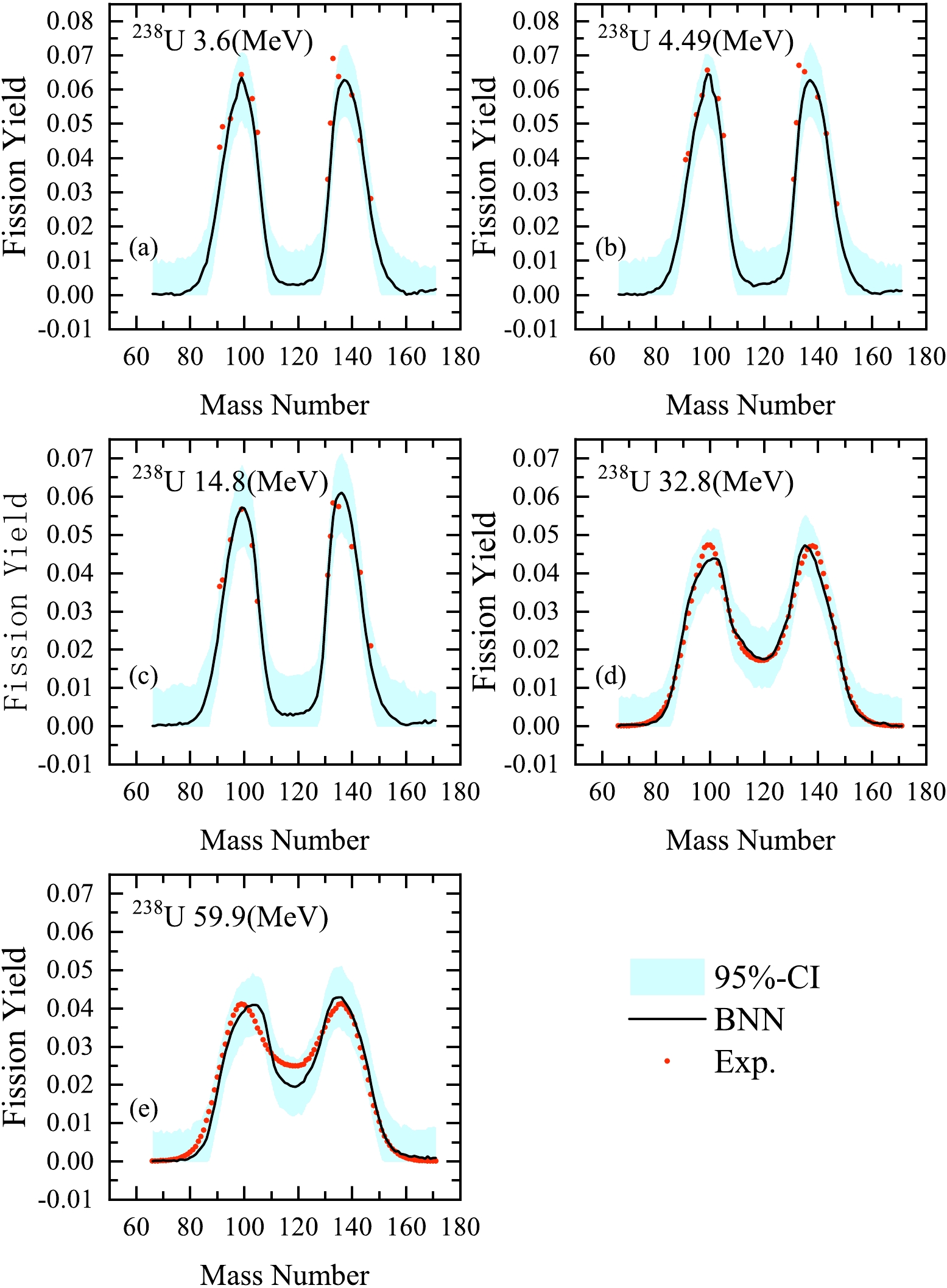
As described above, the neutron energy ranges from 0.053 to 22.5 MeV in the training and test sets. To explore the estimation ability of our BNN at higher excitation energies, the evaluation of
$ ^{238} $ U (n, f) at energies of 32.8 and 59.9 MeV is also shown in Fig. 8(d)−(e). The calculated mass distributions of the fragments are denoted by solid lines. From a comparison of the experimental data with the results evaluated using the BNN, we find that the BNN can give a reasonable evaluation of fission yields at an energy of 32.8 MeV. However, the predictions of fission yields are less satisfactory at 59.9 MeV.We find that the evaluation of the fission fragment mass distributions for
$ ^{238} $ U (n, f) are in good agreement with experimental data at the neutron energy range from 0.50 to 32.8 MeV, perhaps benefiting from the rich$ ^{238} $ U (n, f) data contained in the training set. Although our method can give reasonable results at a higher excitation energy (32.8 MeV) for$ ^{238} $ U (n, f), we still cannot judge the extrapolation ability of the present BNN method. The accumulation of more experimental data in the future will help test the predictive power of this BNN method. In addition, from both the experimental measurements and results of the BNN, it is clear that the asymmetry of distributions persists even at very high excitation energies (approximately 50−60 MeV) of fissioning nuclei.We believe it would be desirable to show some predictions of the dependence of the mass distribution shape on neutron energy. Therefore, predictions are made for the dependence of the shape of the mass distribution for the
$ ^{227,229} $ Th(n, f) and$ ^{238,240} $ Pu(n, f) reactions at different incident-neutron-energies, as shown in Fig. 9. It should be noted that asymmetry of the distributions is predicted even at very high excitation energies (approximately 40 MeV) of fissioning nuclei, presuming that this may be useful for future experiments.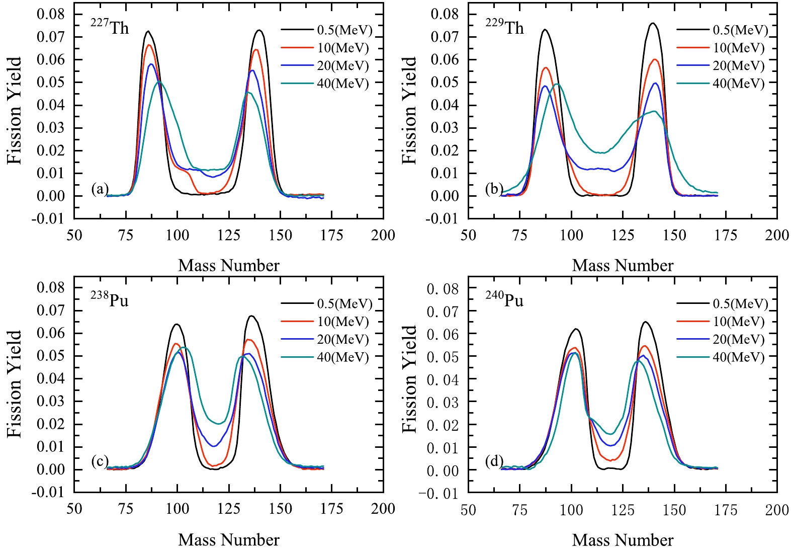
Figure 9. (color online) Calculated mass distributions for the
$^{227,229}$ Th(n, f) and$^{238,240}$ Pu(n, f) reactions at different incident-neutron-energies. -
The BNN method is applied to estimate the fission fragment mass distributions in neutron induced fission with incident energies from 0.0253 to 32.8 MeV. The input for the BNN includes the incident neutron energy, the neutron and charge numbers of the fission nucleus, and the mass numbers of the fragment. From a comparison with the experimental data, it may be concluded that the BNN method is satisfactory for the distribution positions and energy dependencies of fission yields. The fragment mass distributions of several actinides are predicted, presuming that this might help discriminate between all possible future experiments.
Bayesian evaluation of energy dependent neutron induced fission yields
- Received Date: 2023-06-16
- Available Online: 2023-12-15
Abstract: From both the fundamental and applied perspectives, fragment mass distributions are important observables of fission. We apply the Bayesian neural network (BNN) approach to learn the existing neutron induced fission yields and predict unknowns with uncertainty quantification. Comparing the predicted results with experimental data, the BNN evaluation results are found to be satisfactory for the distribution positions and energy dependencies of fission yields. Predictions are made for the fragment mass distributions of several actinides, which may be useful for future experiments.


 DownLoad: