


 Abstract
 HTML
HTML Reference
 Related
 PDF
PDF


-
In 2012, the ATLAS and CMS collaborations reported that a new boson at approximately 125 GeV was discovered at the LHC [1, 2]. It was proved to be the Standard Model (SM)-like Higgs boson, according to its spin,
$ CP $ property, production, and decay performances in Run I and Run II data globally [3–5]. The Higgs boson is related to the electroweak symmetry-breaking mechanism and hierarchy problem and represents an interesting phenomenology in many new physics models. The question of whether there are additional Higgs bosons is natural, important, and remains unsolved. Ten years after the 125-GeV Higgs boson was discovered, experimentalists are still making efforts to search for additional Higgs scalars, even if in the low-mass region.In 2018, the CMS collaboration reported a di-photon excess at approximately 95.3 GeV with a local significance of 2.8 σ [6] and a signal strength of
$ R_{\gamma\gamma}^{\rm{ex}} = \frac{\sigma^{\rm{ex}}(gg \to \phi \to \gamma\gamma)}{\sigma^{\rm{SM}}(gg \to h \to \gamma\gamma)} = 0.6 \pm 0.2 \;. $

(1) Interestingly, the CMS collaboration recently also reported a di-tau excess at
$95- 100$ GeV with a local significance of$2.6- 3.1 \; \sigma$ [7] and a signal strength of$ R_{\tau\tau}^{\rm{ex}} = \frac{\sigma^{\rm{ex}}(gg \to \phi \to \tau^+\tau^-)}{\sigma^{\rm{SM}}(gg \to h \to \tau^+\tau^-)} = 1.2 \pm 0.5 \;. $

(2) Besides, a
$ b\bar{b} $ excess at approximately 98 GeV with a local significance of 2.3 σ was reported from the LEP data approximately twenty years ago [8], whose signal strength is$ R_{bb}^{\rm{ex}} = \frac{\sigma^{\rm{ex}}(e^+e^- \to Z\phi \to Zb\overline b)}{\sigma^{\rm{SM}}(e^+e^- \to Zh \to Zb\overline b)} = 0.117 \pm 0.057 \;. $

(3) Given that the three excesses are close to each other in mass regions and comparable in signal strengths with a SM Higgs boson of the same mass, a series of studies were conducted to interpret them as one additional Higgs-like scalar in new physics models, with [9–12] and without [13–32] di-tau excess.
Supersymmetry (SUSY) [33–35] is a popular theory beyond the SM. The next-to-minimal supersymmetric standard model (NMSSM) [36] includes two Higgs doublets and one singlet, which implies more freedom than the minimal supersymmetric standard model (MSSM) in the Higgs sector [37]. It can naturally accommodate a SM-like Higgs boson at 125 GeV with signal strengths properly fitting the experimental data [38–47]. It can also predict a type of Higgs exotic decay to a pair of additional Higgs scalars lighter than the half mass [48–51]. At the moment, we have three possible excesses in different channels in the
$ 95- 100 $ GeV region. Thus, it is interesting to analyze whether it is possible to interpret all three excesses together in the NMSSM. In this study, we imposed the three excesses from one$ 95- 100 $ GeV Higgs scalar in NMSSM, investigating its status by confronting the excesses. In our calculations, we considered other related constraints including Higgs data, SUSY searches, dark matter relic density, and direct detection.The rest of this paper is organized as follows. In Sec. II, we introduce the Higgs sector in NMSSM and present the relevant analytic equations. In Sec. III, we report and discuss numerical-calculation results. Finally, we draw the main conclusions in Sec. IV.
-
SUSY models are mainly determined by their superpotential and soft-breaking terms. In the NMSSM, they can be written as
$ W = W_{{\rm{MSSM}}}^{\mu\to \lambda \hat{S}} +\kappa \hat{S}^3 /3, $

(4) $ \begin{aligned}[b] V_{\rm{soft}} =& \tilde m_{H_u}^2|H_u|^2 + \tilde m_{H_d}^2|H_d|^2 +\tilde m_S^2|S|^2 \\ & +( \lambda A_{\lambda} SH_u\cdot H_d +\kappa A_{\kappa} S^3 /3 + {\rm h.c.}) \,, \end{aligned}$

(5) where
$ W_{{\rm{MSSM}}}^{\mu\to \lambda \hat{S}} $ is the MSSM superpotential with the μ-term generated effectively by the Vacuum Expectation Value (VEV) of singlet field, and$ \tilde{m}_{H_u} $ ,$ \tilde{m}_{H_d} $ ,$ \tilde{m}_{S} $ ,$ A_\lambda $ , and$ A_\kappa $ are soft-breaking parameters.$ \hat{H_u} $ ,$ \hat{H_d} $ are the SU(2) doublet and$ \hat{S} $ is the singlet Higgs superfields; after obtaining VEVs, the scalar fields can be expressed as$ \begin{aligned}[b] & H_{u}=\left( \begin{array}{c} H^+_{\rm{u}} \\ v_{u}+ \dfrac{\phi_{u}+ {\rm i}\varphi_{u}}{\sqrt{2}} \\ \end{array} \right) , \\& H_{d}=\left( \begin{array}{c} v_{d}+ \dfrac{\phi_{d}+ {\rm i} \varphi_{d}}{\sqrt{2}} \\ H^-_{\rm{d}} \\ \end{array} \right) , \quad S=v_{s}+ \dfrac{\phi_{s}+{\rm i}\varphi_{s}}{\sqrt{2}} \,,\end{aligned} $

(6) and
$ \tan\beta \equiv v_u/v_d $ .The three gauge-eigenstate scalars
$ \{\phi_u, \phi_d, \phi_s\} $ mix to form three CP-even mass-eigenstate Higgs scalars$ \{h_1, h_2, h_3\} $ , with mass order$ m_{h_1}<m_{h_2}<m_{h_3} $ and mixing matrix$ \{S_{ij}\}_{3\times 3} $ :$\left( {\begin{array}{*{20}{c}} {{h_1}}\\ {{h_2}}\\ {{h_3}} \end{array}} \right) = \left( {\begin{array}{*{20}{c}} {{S_{11}}}&{{S_{12}}}&{{S_{13}}}\\ {{S_{21}}}&{{S_{22}}}&{{S_{23}}}\\ {{S_{31}}}&{{S_{32}}}&{{S_{33}}} \end{array}} \right)\left( {\begin{array}{*{20}{c}} {{\phi _u}}\\ {{\phi _d}}\\ {{\phi _s}} \end{array}} \right). $

(7) The reduced couplings of
$ h_1 $ to up- and down-type fermions, and massive gauge bosons, are given by$ \begin{aligned}[b]& c_t=S_{11}/\sin\beta \,, \\& c_b=S_{12}/\cos\beta \,, \\& c_V=S_{11}\sin\beta +S_{12}\cos\beta \,.\end{aligned} $

(8) The loop-induced coupling to gluons
$ c_g $ is mainly determined by$ c_t $ and light colored SUSY particles, and that of photon$ c_\gamma $ is mainly determined by$ c_t $ ,$ c_V $ , and light charged SUSY particles. -
In the conducted calculations, we first scanned the parameter space of NMSSM with the public code
$ \mathsf{NMSSMTools\_5.6.1} $ [52–54] under a series of experimental and theoretical constraints1 . The parameter space we considered is defined as follows:$\begin{aligned}[b]& 0.1 < \lambda< 0.7, \; \; \; |\kappa| < 0.7,\; \; \; 1<\tan\beta < 60, \\& M_{0},|M_{3}|,|A_{0}|,|A_{\lambda}|,|A_{\kappa}|< 10 {\rm \; TeV} \,,\\& \mu_{\rm{eff}}, |M_{1}|, |M_{2}|< 1 {\rm \; TeV} \,. \end{aligned} $

(9) Note that the NMSSM considered in this study is GUT-scale constrained, where both Higgs and gaugino masses are considered non-universal. Thus,
$ M_0 $ and$ A_0 $ are the unified sfermion masses and trilinear couplings in the sfermion sector, and$ M_{1,2,3} $ are the gaugino masses at the GUT scale. The three non-universal Higgs masses at the GUT scale were calculated from the minimization equations, with λ, κ, and$ \mu_{\rm{eff}}\equiv \lambda v_S $ at the SUSY scale as the input parameters. The parameter$ \mu_{\rm{eff}} $ was chosen to be positive to interpret the muon$ g-2 $ anomaly. One sign in three of$ M_{1,2,3} $ can be absorbed in a field redefinition [35]. The sign of$ M_3 $ can have other effects (see Ref. [55]).The constraints we imposed include (i) A SM-like Higgs boson
2 with mass at approximately 125 GeV (i.e., 123 − 127 GeV) and signal strengths in agreement with the latest data in$\mathsf{HiggsSignals}-\mathsf{2.2.3beta}$ [56, 57]; (ii) exclusion limits in the search for additional Higgs bosons at the LEP, Tevatron, and LHC, collected from$\mathsf{HiggsBounds}- \mathsf{5.10.1}$ [58–60]; (iii) upper limit of dark matter relic density with uncertainty ($ \Omega h^2 \leq 0.131 $ ) [61–63] and direct detections [64], where the quantities were calculated using$\mathsf{micrOMEGAs}$ in$\mathsf{NMSSMTools}$ ; (iv) exclusion limits in SUSY searches imposed in$\mathsf{SModelS}- \mathsf{v2.1.1}$ [65–68], such as electroweakinos in multilepton channels [69, 70] and gluino and first-two-generation squarks [71]; and (v) theoretical constraints of vacuum stability and no Landau pole below GUT scale [54].To interpret the CMS di-photon and di-tau, and LEP
$ b\bar{b} $ excesses together, we also require a light Higgs boson of$95-100\;{\rm{GeV}}$ . For the surviving samples, we defined a chi-square quantity$ \chi^2_{\gamma\gamma+\tau\tau+bb} $ to describe its ability to interpret the three excesses globally:$ \chi^2_{\gamma\gamma+\tau\tau+bb} = \chi_{\gamma\gamma}^2 + \chi_{\tau\tau}^2 + \chi_{bb}^2 \, , $

(10) where
$ \chi_{i}^2 = \left( \frac{R_{i}-\bar{R}_{i}^{\rm{ex}}} {\delta R_{i}^{\rm{ex}}} \right)^2 \,, $

where
$ i=\gamma\gamma,\tau\tau,bb $ ,$ R_{i} $ denotes the corresponding theoretical signal strength of our samples, and$ \bar{R}_{i}^{\rm{ex}} $ and$ \delta R_{i}^{\rm{ex}} $ denote the corresponding experimental mean and error values, respectively. For$ \chi^2_{\gamma\gamma+\tau\tau+bb}\le 8.03 $ , the surviving samples can interpret the three excesses globally at$ 2\sigma $ level. They will be called 'global$ 2\sigma $ samples' or alternatively '$ 2\sigma $ samples' hereafter. Note that for surviving samples, the minimum value of$ \chi^2_{\gamma\gamma+\tau\tau+bb} $ is 5.37; therefore, there are no samples satisfying the three excesses at$ 1\sigma $ level globally ($ \chi^2_{\gamma\gamma+\tau\tau+bb} < 3.53 $ ). Table 1 lists the parameter regions for the$ 2\sigma $ and all surviving samples.$ 2\sigma $ samples

all surviving samples λ 0.11−0.58 0.10−0.69 κ −0.60− 0.55 −0.56−0.61 tanβ 6.4−45.2 2.6−50.6 $ \mu_{\rm{eff}} $ /GeV

139−487 102−978 $ M_0 $ /TeV

0−9.5 0−10.0 $ A_0 $ /TeV

−5.0−6.5 −8.3−9.3 $ M_1 $ /GeV

−805−199 −1000−993 $ M_2 $ /TeV

−6.7−1.0 −10.0−2.4 $ M_3 $ /TeV

−3.4−6.4 −4.8−9.8 $ A_\lambda $ /TeV

1.4−10.0 0.1−10.0 $ A_\kappa $ /TeV

−2.0−2.4 −2.7−2.7 Table 1. Parameter regions for
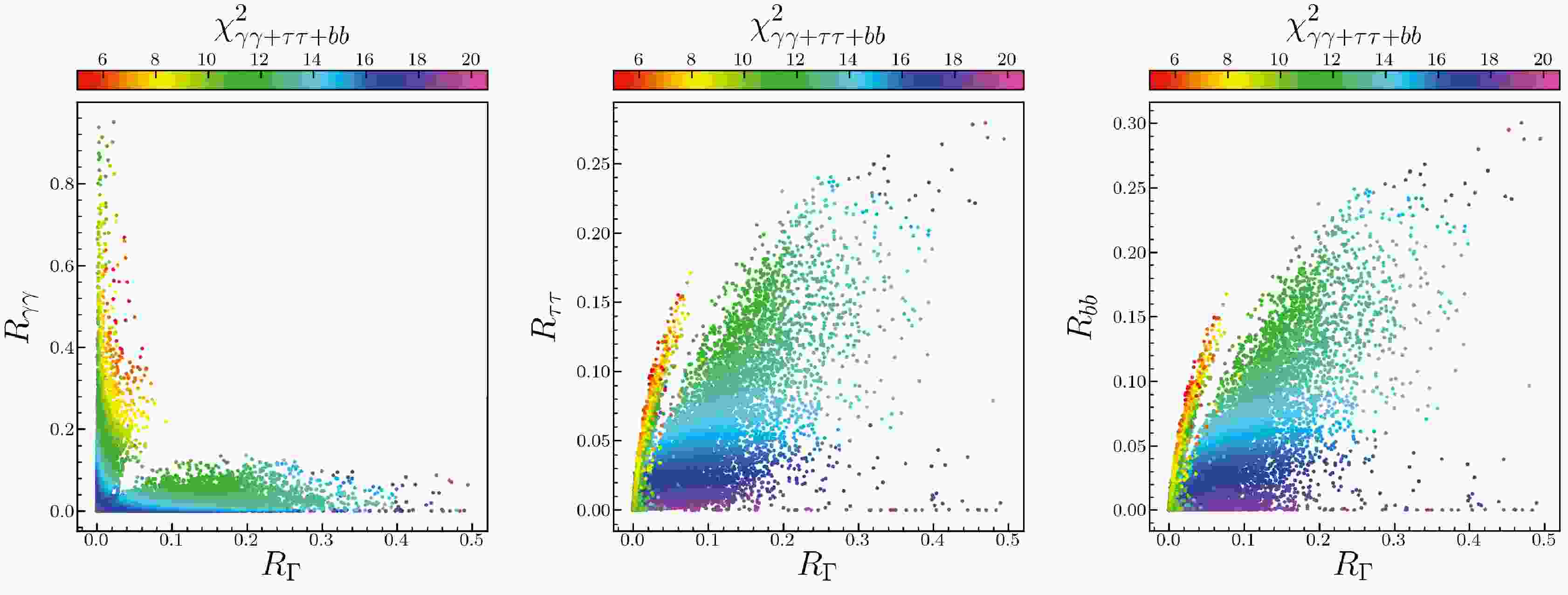
$ 2\sigma $ ($ \chi^2_{\gamma\gamma+\tau\tau+bb}\le 8.03 $ ) and all surviving samples.Figure 1 shows the surviving samples on the signal strengths
$ R_{\gamma \gamma} $ ($ gg \to h_1 \to \gamma\gamma $ ),$ R_{\tau \tau} $ ($ gg \to h_1 \to \tau\bar{\tau} $ ), and$ R_{bb} $ ($ e^{+}e^{-} \to Zh_1 \to Zb\bar{b} $ ) versus width ratio$ R_{\Gamma} $ (total decay width of$ h_1 $ divided by that of a SM Higgs of the same mass) planes, with colors denoting$ \chi^2_{\gamma\gamma+\tau\tau+bb} $ . This figure shows that the low-mass excess data are powerful in distinguishing the surviving samples. For the$ 2\sigma $ samples,$ R_{\Gamma}\lesssim 0.1 $ ,$ 0.2\lesssim R_{\gamma\gamma}\lesssim 0.8 $ , and$ R_{\tau\tau}, R_{b b} \lesssim0.2 $ . The surviving samples can be clearly sorted into two regions:$ R_{\Gamma}\lesssim 0.1 $ and$ R_{\gamma\gamma}\lesssim 0.2 $ . Note that the$ 2\sigma $ samples can be only located in the former. Hereafter, to compare with the$ 2\sigma $ samples in the former region, we consider the$ 3\sigma $ samples, or samples with$ 8.03\lesssim \chi^2_{\gamma\gamma+\tau\tau+bb}\lesssim 14.16 $ in the latter region, called small-$ R_{\gamma\gamma} $ samples. Note from the middle and right planes that for the$ 2\sigma $ samples,$0.04\lesssim R_{\tau\tau},\; R_{bb}\lesssim 0.16$ , while for the small-$ R_{\gamma\gamma} $ samples,$0.05\lesssim R_{\tau\tau}, \;R_{bb}\lesssim 0.25$ . In combination with experimental data, it can be observed that the$ 2\sigma $ samples mainly fit well with the CMS di-photon excess, and small-$ R_{\gamma\gamma} $ samples mainly fit well with the LEP$ Zb\bar{b} $ excess. The CMS di-tau excess has so large uncertainty that it cannot be dominant in our samples.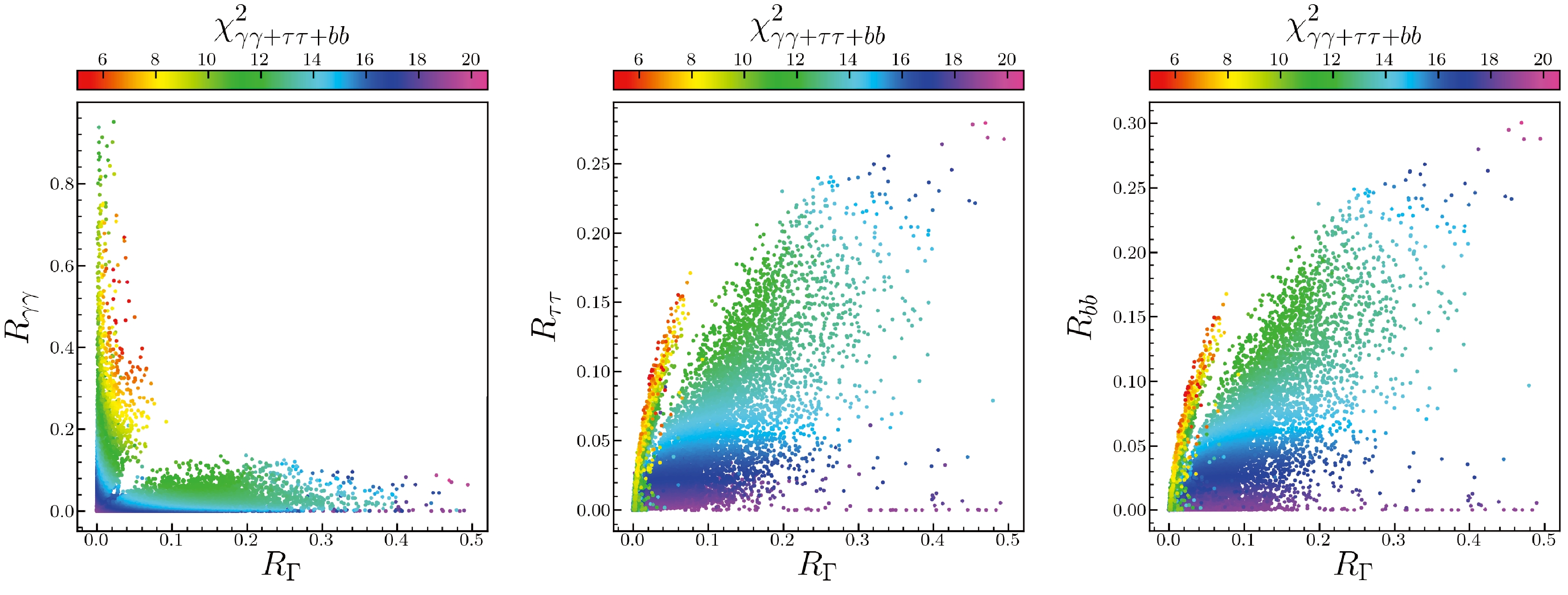
Figure 1. (color online) Surviving samples on the planes of signal strength
$ R_{\gamma \gamma} $ ($ gg \to h_1 \to \gamma\gamma $ ) (left),$ R_{\tau\tau} $ ($ gg \to h_1\to \tau \bar{\tau} $ ) (middle),$ R_{bb} $ ($ e^{+}e^{-}\to Zh_1\to Zb\bar{b} $ ) (right) versus width ratio$ R_{\Gamma} $ , respectively; the colours indicate$ \chi^2_{\gamma\gamma+\tau\tau+bb} $ .The signal strengths are related to the reduced couplings by
$ R_{\gamma \gamma} = c_g^2c_{\gamma}^2/R_{\Gamma} \,, \;\; R_{\tau\tau} = c_g^2c_{\tau}^2/R_{\Gamma} \,,\;\; R_{bb} = c_V^2 c_b^2/R_{\Gamma} \,. $

(11) Figure 2 shows the surviving samples on the signal strengths versus reduced coupling planes, with colors denoting again
$ \chi^2_{\gamma\gamma+\tau\tau+bb} $ . Note that the reduced couplings can be sorted into two classes:$ |c_{\gamma}| \approx |c_g| \approx |c_t| \approx |c_V| $ and$ c_b \approx c_{\tau} $ . Note also that the width ratio is determined by$ c_b^2 $ , and the dominant branching ratio of the light scalar is that of$ b\bar{b} $ . The signal strengths can be approximately rewritten as
Figure 2. (color online) Same as in Fig. 1, but on the planes of signal strength versus reduced coupling:
$ R_{\gamma\gamma} $ versus$ c_{\gamma} $ (upper left),$ R_{\gamma\gamma} $ versus$ c_{g} $ (lower left),$ R_{\tau\tau} $ versus$ c_{\tau} $ (upper middle),$ R_{\tau\tau} $ versus$ c_{t} $ (lower middle),$ R_{bb} $ versus$ c_{b} $ (upper right),$ R_{bb} $ versus$ c_{V} $ (lower right).$ R_{\gamma \gamma} \approx c_t^4 / c_b^2 \,, \;\;\;\;R_{\tau\tau} \approx c_t^2 \,, \;\;\;\; R_{bb} \approx c_t^2 \,, $

(12) where the small width ratio
$ R_{\Gamma} $ , or approximate$ c_b^2 $ , can increase the di-photon rate but cannot increase the$ b\bar{b} $ and di-tau rates. Thus,$ \chi^2_{\gamma\gamma+\tau\tau+bb} $ can be approximately expressed as$ \begin{aligned}[b] \chi^2_{\gamma\gamma+\tau\tau+bb} \approx & \left[25\left(\frac{c_t}{c_b}\right)^4 + 311.8 \right] c_t^4 \\ & - \left[30\left(\frac{c_t}{c_b}\right)^2 + 81.6 \right] c_t^2 + 19.0 \,. \end{aligned} $

(13) According to Fig. 2, for
$ 2\sigma $ samples, the light scalar has negative reduced couplings to fermions and W/Z bosons, with$ 0.3\lesssim -c_t \lesssim 0.4 $ and$0.05 \lesssim -c_b \lesssim 0.3$ ; for small-$ R_{\gamma\gamma} $ samples, the reduced couplings are positive, with$ 0.25\lesssim c_t \lesssim 0.45 $ and$ 0.25 \lesssim c_b \lesssim 1 $ . Note also from Eq. (13) that when$ c_t=0 $ or$ c_t=0.5 $ with$ c_b=1 $ ,$ \chi^2_{\gamma\gamma+\tau\tau+bb} \approx 19 $ ; when$ |c_t|=2|c_b|=\sqrt{0.1} $ ,$ \chi^2_{\gamma\gamma+\tau\tau+bb} \approx 6 $ .Figure 3 shows the surviving samples on the
$ S_{12} $ -$ S_{11} $ ,$ \tan\beta $ -$ S_{12} $ and$ c_t $ -$ c_b $ planes. According to Fig. 3, when$ c_t, c_b \lesssim 0 $ , or the couplings to quarks are flipped in sign,$ |c_t/c_b| \gtrsim 1 $ , which defines the region where most$ 2\sigma $ samples are located in; otherwise$ |c_t/c_b| \lesssim 1 $ , and$ R_{\gamma\gamma} $ will be smaller. Combining Fig. 3 and Eq. (8), and given that$ \tan\beta\gg 1 $ and$ |S_{12}|\ll 1 $ , we can safely state that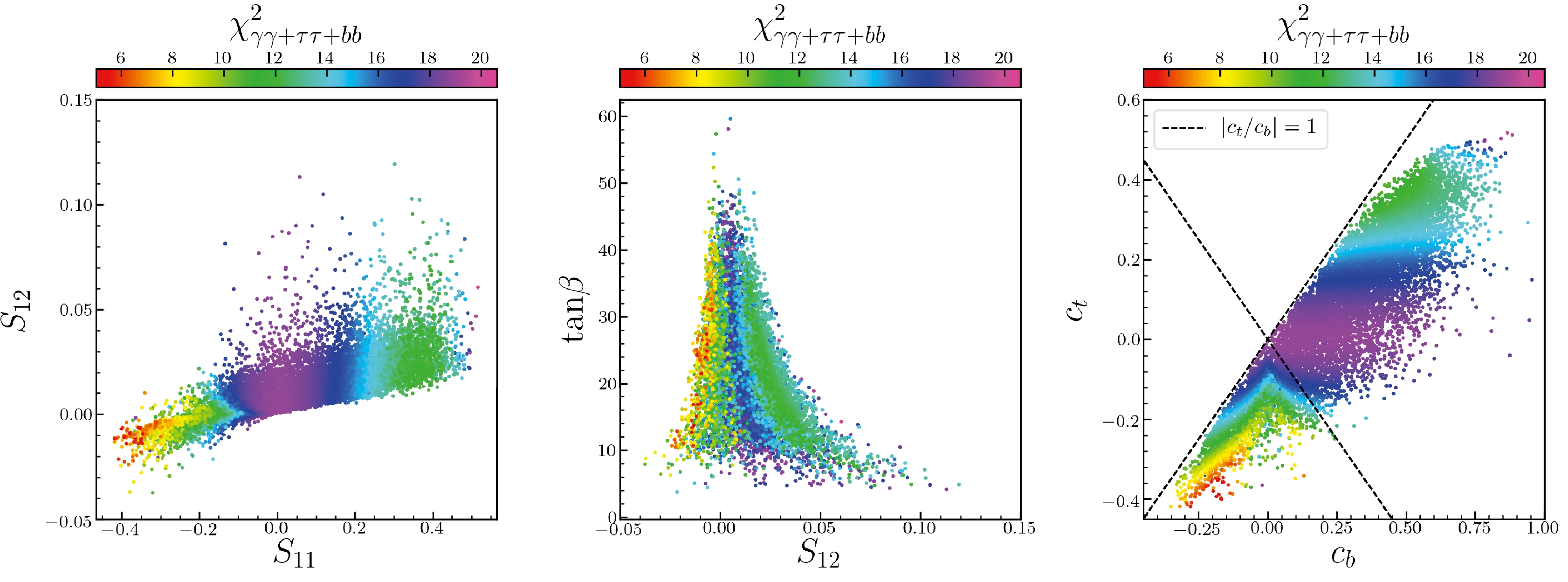
Figure 3. (color online) Same as in Fig. 1, but on
$ S_{12} $ versus$ S_{11} $ (left),$ \tan\beta $ versus$ S_{12} $ (middle), and$ c_t $ versus$ c_b $ (right) planes, respectively.$ c_V \approx c_t \approx S_{11} \,, \quad c_b \approx S_{12}\tan\beta \,. $

(14) It can also be observed from Fig. 3 that for the
$ 2\sigma $ samples,$ |S_{11}| \gg |S_{12}| $ , which means that the lightest Higgs boson is mainly mixed by the singlet and up-type doublet fields. Departing from this, in the wrong sign limit [72, 73] of the type-II two Higgs doublet model, the lighter Higgs boson is mixed by the up- and down-type doublets fields. We also checked that the absence of the case$ c_t \gtrsim c_b $ in Fig. 3 results from choosing a positive$ \mu_{\rm{eff}} $ , which is favored by the muon$ g-2 $ constraint. Given that the down-type doublet-like Higgs boson in NMSSM needs to be much heavier than the other two Higgs bosons to escape the constraints,$ S_{12} $ , or the mixing between singlet and down-type doublet, should be very small compared with$ S_{11} $ ; thus, the cases of$ c_t \lesssim 0 $ and$ c_b \gtrsim 0 $ are not favored.Considering that the mass region of excesses is close to the Z boson mass, we consider the scalar production associated with a top quark pair to reduce the backgrounds, with the signal strengths expressed as follows:
$ R_{t\overline t\gamma\gamma} = c_t^2c_{\gamma}^2/R_{\Gamma} \,, \;\; R_{t\overline t\tau \overline\tau} = c_t^2c_{\tau}^2/R_{\Gamma} \,,\;\; R_{t\overline tb\overline b} = c_t^2 c_b^2/R_{\Gamma} \,. $

(15) Figure 4 shows the surviving samples on the planes of signal strengths of top-quark-pair associated channels versus the three excess channels. Note that
$ R_{t\bar{t}\gamma\gamma}\approx R_{\gamma\gamma} $ ,$ R_{t\bar{t}\tau\bar{\tau}}\approx R_{\tau\tau} $ ,$R_{t\bar{t}b\bar{b}}\approx R_{bb}$ . There is a small difference, especially between top-pair-associated and gluon-gluon-fusion channels. For$ 2\sigma $ samples, the latter is slightly larger than the former; while for the small-$ R_{\gamma\gamma} $ samples, the former is slightly larger than the latter. The difference comes from the contributions of squarks, and they are positive or negative depending on$ c_t $ , that is, the reduced couplings to the top quark. The difference is small because of the high mass bounds of squarks [74] according to SUSY search results. As a comparison, new light colored particles can contribute significantly to the gluon-gluon-fusion channel [75].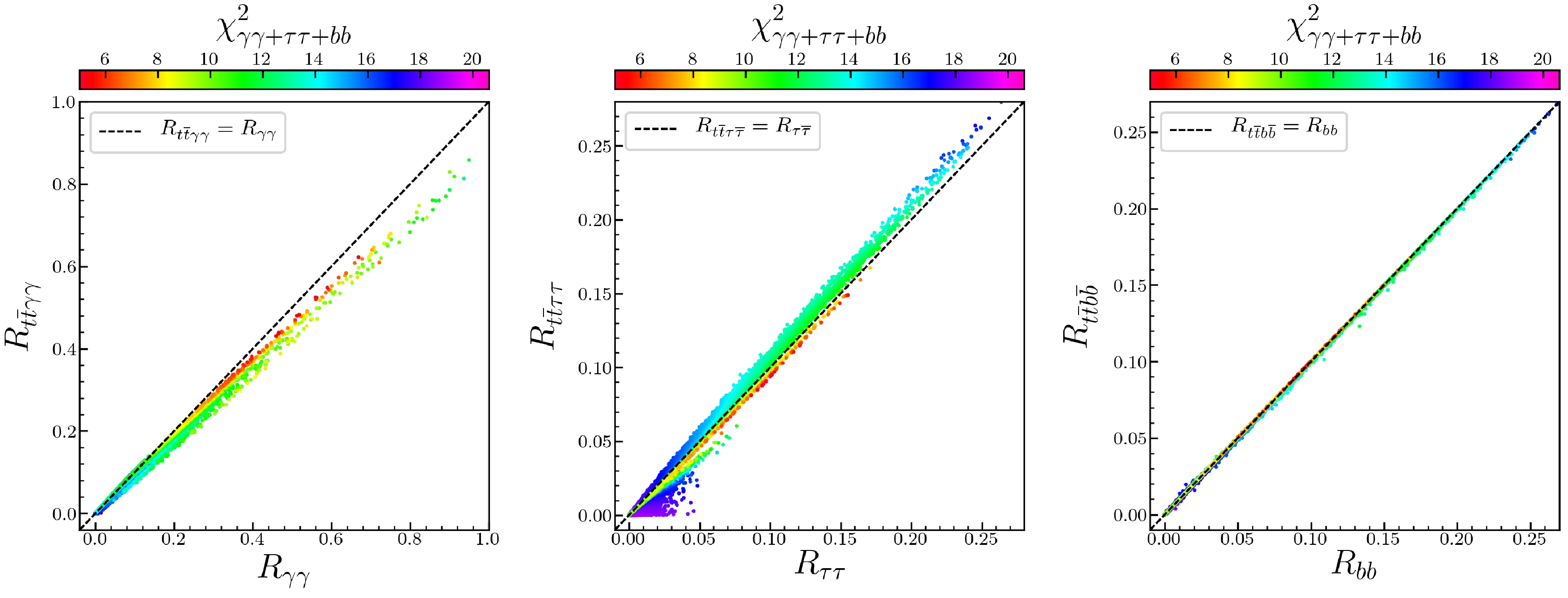
Figure 4. (color online) Same as in Fig. 1, but on the planes of signal strengths in top-quark-pair associated channels versus those of existing excess channels:
$ R_{t\bar{t}\gamma\gamma} $ versus$ R_{\gamma\gamma} $ (left),$ R_{t\bar{t}\tau\tau} $ versus$ R_{\tau\tau} $ (middle) and$ R_{t\bar{t}b\bar{b}} $ versus$ R_{bb} $ (right) planes.Table 2 lists detailed information of eight representative benchmark points for further study, where
$ \chi^2_{125} $ and$ P_{125} $ are the chi-square and P value from 125 GeV Higgs data of 111 groups (the number of degrees of freedom is 111). Note that for a SM Higgs of 125.09 GeV,$ \chi^2_{125}=89.7 $ and$ P_{125}=0.932 $ . This table shows that it is difficult to satisfy the 125 GeV Higgs data and$ 95-100\;{\rm{GeV}} $ excesses simultaneously at the$ 2\sigma $ level. For instance, concerning Point P4, for the$ 95-100\;{\rm{GeV}} $ excesses globally satisfied at the$ 2\sigma $ level, the 125 GeV Higgs data can be at 78.4%, which is worse than that of a SM Higgs boson at$ 125\;{\rm{GeV}} $ .P1 P2 P3 P4 P5 P6 P7 P8 λ 0.315 0.348 0.335 0.271 0.297 0.165 0.116 0.339 κ 0.128 0.138 0.102 0.052 −0.121 −0.051 0.044 0.544 tanβ 30.8 30.5 31.8 25.1 21.2 6.4 11.1 14.7 $ \mu_{\rm{eff}} $ /GeV

272 284 308 263 288 391 214 232 $ M_0 $ /GeV

1503 1824 2342 1954 3415 303 790 335 $ A_0 $ /GeV

1804 1947 867 1081 949 −1717 1653 1617 $ M_1 $ /GeV

−49.6 −50.1 −19.7 −18.1 −83.9 −75.4 −63.7 −622 $ M_2 $ /GeV

−2061 −2363 −3892 −2862 −302 249 −84 742 $ M_3 $ /GeV

2877 3037 4948 4920 2992 1439 2004 2574 $ A_\lambda $ /GeV

7881 8510 8077 4474 6395 2212 2807 2745 $ A_\kappa $ /GeV

1610 2224 2111 837 1797 572 −107 −3538 $ m_{h_1} $ /GeV

96.5 95.0 95.2 95.6 98.3 96.9 98.8 96.4 $ m_{h_2} $ /GeV

124.9 125.2 126.0 125.7 125.9 125.7 126.1 126.0 $ S_{11} $ 

−0.343 −0.340 −0.287 −0.255 −0.220 0.383 0.399 0.336 $ S_{12} $ 

−0.0050 −0.0046 −0.0033 −0.0033 −0.0023 0.0695 0.0438 0.0405 $ c_t $ 

−0.344 −0.341 −0.287 −0.256 −0.220 0.388 0.400 0.337 $ c_V $ 

−0.343 −0.340 −0.287 −0.255 −0.220 0.390 0.401 0.338 $ c_b $ 

−0.153 −0.139 −0.104 −0.082 −0.050 0.451 0.489 0.597 $ c_\tau $ 

−0.153 −0.139 −0.104 −0.082 −0.050 0.451 0.489 0.597 $ |c_g| $ 

0.356 0.354 0.299 0.268 0.232 0.385 0.395 0.324 $ |c_\gamma| $ 

0.382 0.381 0.324 0.291 0.255 0.377 0.376 0.288 $ R_\Gamma $ 

0.0200 0.0172 0.0107 0.0074 0.0046 0.1178 0.1396 0.1953 $ R_{\gamma\gamma} $ 

0.548 0.618 0.510 0.472 0.455 0.106 0.096 0.026 $ R_{\tau\tau} $ 

0.088 0.082 0.053 0.037 0.017 0.152 0.162 0.113 $ R_{bb} $ 

0.083 0.077 0.049 0.035 0.016 0.156 0.167 0.123 $ R_{t\bar{t}\gamma\gamma} $ 

0.509 0.571 0.469 0.431 0.410 0.108 0.098 0.029 $ R_{t\bar{t}\tau\bar{\tau}} $ 

0.082 0.076 0.049 0.034 0.016 0.155 0.166 0.123 $ R_{t\bar{t}b\bar{b}} $ 

0.083 0.077 0.050 0.035 0.016 0.154 0.166 0.122 $ \chi^2_{\gamma\gamma+\tau\tau+bb} $ 

5.37 5.50 6.87 7.91 9.26 10.95 11.42 12.96 $ \chi_{125}^2 $ 

116.4 116.7 103.8 99.1 95.7 99.2 99.4 90.9 $ P_{125} $ 

0.344 0.337 0.673 0.784 0.850 0.782 0.777 0.919 $ m_{\tilde{\chi}^0_1} $ 

44.53 46.01 43.15 43.00 60.38 43.92 44.98 227.96 $ \Omega h^2 $ 

0.0213 0.0719 0.0566 0.0187 0.0524 0.0862 0.0086 0.0065 $ Br(h_2 \to \tilde{\chi}^0_1 \tilde{\chi}^0_1) $ 

0.0027% 0.0016% 0.022% 0.085% 0.15% 1.03% 0.028% 0.00% Table 2. Eight benchmark points for the surviving samples.
Finally, we elaborate on dark matter, invisible Higgs decay, and electroweakino searches:
● For benchmark points P1-P7, the dark matter is bino-like, and the main annihilation mechanism is
$ Z/h_2 $ funnel. The mass of dark matter is different from$ M_1 $ because the parameters$ M_{1,2,3} $ are defined at the GUT scale. There are correlations between parameters at GUT and SUSY scales, similar to those presented in Appendix A of a previous study of ours [55].● We considered the constraint of invisible Higgs decay with the code
$\mathsf{HiggsBounds}$ ; the corresponding experimental data are provided in Refs. [76, 77]. For benchmark points P1-P7, the invisible Higgs decay$ Br(h_2\to\tilde{\chi}^0_1 \tilde{\chi}^0_1) $ is approximately below 1%, because the large invisible ratios are not favored by both 125 and$95-100\;{\rm{GeV}}$ Higgs data.● We also imposed constraints from SUSY searches with the code
$\mathsf{SModelS}$ . For benchmark point P8, the dark matter is Higgsino-like and the main annihilation mechanism is$ W^\pm/Z $ exchanges. This point can escape the constraints from searches for electroweakinos in Ref. [78] because of its compressed mass spectrum and multiple decay modes. In the low mass region, it has SUSY particles such as Higgsino-like charginos and neutralinos of approximately$ 230\;{\rm{GeV}} $ , bino-like neutralino of$ 390\;{\rm{GeV}} $ , wino-like charginos and neutralinos of approximately$ 590\;{\rm{GeV}} $ ,$ \tilde{\tau}_1 $ of$ 246\;{\rm{GeV}} $ ,$ \tilde{\nu}_{\tau} $ of$ 353\;{\rm{GeV}} $ ,$ \tilde{\mu}_1 $ of$ 478\;{\rm{GeV}} $ , and$ \tilde{\nu}_{\mu} $ of$ 472\;{\rm{GeV}} $ . -
In this study, we considered a light Higgs boson in the NMSSM to interpret the CMS di-photon and di-tau excesses, as well as the LEP
$ b\bar{b} $ excess, in the$95-100\;{\rm{GeV}}$ mass region. We first scanned the parameter space and considered a series of constraints, including Higgs, dark matter, and SUSY searches. Then for each surviving sample, we calculated a chi-square considering its global fit to the three excess data. We focused on two respective types of samples:$ 2\sigma $ and small-$ R_{\gamma\gamma} $ . Finally, we drew the following conclusions:● In NMSSM, it is difficult to satisfy the
$ 95\sim 100\;{\rm{GeV}} $ excesses simultaneously (not possible globally at$ 1\sigma $ level, or simultaneously at$ 2\sigma $ level).● The global fit of the light Higgs boson to the three excesses is mainly determined by its couplings to up- and down-type fermions, which can be approximately expressed as in Eq. (13).
● The global
$ 2\sigma $ samples have negative reduced couplings to fermions and massive vector bosons, while they are positive for the small-$ R_{\gamma\gamma} $ ones.● The global
$ 2\sigma $ samples have a decay width smaller than one-tenth of the corresponding SM value, which can increase its di-photon rate but cannot increase its di-tau rate.● The small-
$ R_{\gamma\gamma} $ samples can have$ Zb\bar{b} $ signal right fit to the LEP$ b\bar{b} $ excess, but have smaller di-photon and di-tau rates.● The top-quark-pair associated signal strengths are nearly equal to those of the three exciting excesses, respectively.
-
Fig. A1 shows the error level between the approximated chi-square and complete ones in Eq. (13). Note that
$ c_V\approx c_t $ is a very good approximation. For most samples, given that the charged Higgs bosons and most SUSY particles are heavy, their contributions to the loop-induced couplings$ c_g $ ($ c_\gamma $ ) are much smaller than those of the SM particles top quark (and W boson). Thus,$ c_g $ ($ c_\gamma $ ) are mainly determined by the coupling of the top quark,$ c_t $ (and that of the W boson,$ c_V $ ). Given that$ c_V\approx c_t $ , for most samples we have$ c_\gamma \approx c_V\approx c_t \approx c_g $ . According to Fig. A1, the error level between the approximate chi-square and complete ones in Eq. (13) are below 5% for most samples and approximately 15% at most for all. Therefore, Eqs. (12) and (13) are good approximations for most samples, with only two variable quantities.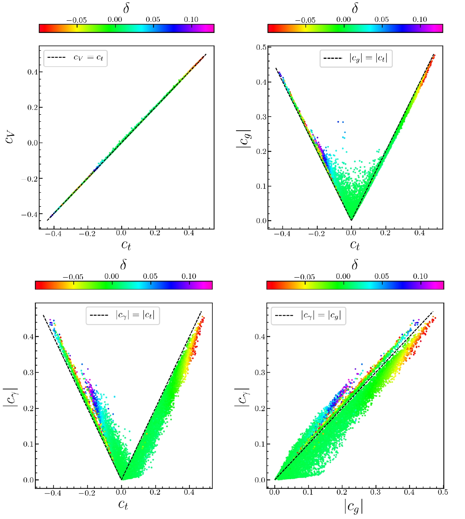
Figure A1. (color online) Surviving samples on the planes of
$ c_V $ (upper left),$ |c_g| $ (upper right) and$ |c_{\gamma}| $ (lower left) versus$ c_t $ , and$ |c_\gamma| $ versus$ |c_g| $ (lower right), with colors indicating the error ratio δ between the approximated and complete ones in Eq. (13).
Light Higgs boson in the NMSSM confronted with the CMS di-photon and di-tau excesses
- Received Date: 2023-07-14
- Available Online: 2023-12-15
Abstract: In 2018, the CMS collaboration reported a di-photon excess at approximately 95.3 GeV with a local significance of 2.8 σ. Interestingly, the CMS collaboration also recently reported a di-tau excess at


 DownLoad: