


 Abstract
 HTML
HTML Reference
 Related
 PDF
PDF


-
Black holes (BHs) are one of the most remarkable phenomena in our Universe. First, we discuss BHs as an essential part of the classical theory of physics. The classical theory of gravity is Einstein's theory of general relativity (GR), which defines both time and space. BHs were first assumed to only exist in theory, and despite the fact that their models were thoroughly studied, many scientists, including Einstein, had doubts about whether they actually existed. In this instance, it was only logical to investigate whether Einstein's theory of gravity explains the idea of time and space surrounding a massive object such as a star. Schwarzschild found a solution to this issue that essentially considers the mass of all stationary round objects. However, unexpected things occur when the entire mass of an object is contained within a certain radius, known as the Schwarzschild radius. When an event horizon occurs at the Schwarzschild radius, the term "BH" is used.
It has been established that BHs and other astronomical objects acquire mass through a procedure called accretion. As a key concept in astrophysics, the accretion phenomenon that encompasses tremendous gravitating objects is essential for understanding a variety of astrophysical behaviors and assumptions, including the formation of super-massive BHs (SMBHs), star formation, emitted radiation of X-rays through the luminosity of quasars, and compact star binaries [1−3]. Because it involves various significant problems of general relativistic magnetohydrodynamics, including radiation, turbulence, and nuclear burning, the accretion of matter is a reliable yet immensely complex astrophysical method. To properly explain the general accretion processes, it is useful to characterize the problem using particular presumptions or by assuming some fundamental requirements.
The basic accretion phenomenon has been illustrated by Bondi [4] for a spherically symmetric object, which implies that an infinitely massive homogeneous gas cloud continuously accretes onto a compact object such as a BH. The Bondi approach is founded on the Newtonian theory of gravity. The steady-state spherically symmetric flow of test fluids into a Schwarzschild BH was then investigated in the framework of GR by Michel [5]. Subsequently, the concept of relativistic accretion on compact objects was further investigated by Shapiro and Teukolsky [6]. Furthermore, Babichev et al. [7] observed that if phantom energy is allowed to accrete onto a BH during the accretion process, the mass of the BH may decrease. The significant reduction in the BH mass by phantom accretion transforms it into a naked singularity, as illustrated by Jamil et al. [8]. Debnath [9] extended Babichev et al.'s [7] idea of static accretion onto a general class of spherically symmetric BHs by investigating how the cosmological constant would affect the rate of accretion. Ficek [10] investigated the Bondi-type accretion in the Reissner-Nordstrom-(anti) de-Sitter spacetime (RN-AdS). Using the methods outlined in Ficek [10], the process of accretion onto the RN-AdS BH with a global monopole was investigated by Ahmed et al. [11]. They extended their previous research to accretion onto BHs [12, 13] in the
$ f (R) $ and$ f (T) $ modified theories of gravity. Azreg-Ainou [14] discovered general relativistic dust accretion for stationary rotating BHs. The relativistic dust accretion of charged particles onto Kerr-Newman BHs has been thoroughly studied by Schroven [15]. There have been several studies devoted to exploring accretion phenomena for various space-times, including the work of Giddings and Mangano [16], Sharif and Abbas [17], John et al. [18], Ganguly et al. [19], Bahamonde and Jamil [20], and Yang [21].The transonic accretion process and the existence of the sonic point (or critical point) have a significant impact on spherical accretion onto BHs. The accretion flow changes at the sonic point from subsonic to supersonic. The sonic points in specific BH space-times tend to be close to the horizon. It is important and exciting to study the small region close to the sonic point because it is inextricably connected to current research on gravitational and electromagnetic wave spectra. Therefore, study of the spherical accretion problem can not only help improve our understanding of the accretion process in various BHs but also, more importantly, provide a unique viewpoint on how to obtain the nature of BH space-time in the presence of strong gravity.
In this study, we investigate astrophysical accretion in the vicinity of a static and spherically symmetric hairy BH within the framework of gravitational decoupling (GD). In GR, the minimal geometric deformation (MGD) technique has been extensively used to achieve GD, in which the primary objective is to obtain exact solutions from a perfect fluid source. This technique was recently implemented to extract exact solutions from the Schwarzschild vacuum metric in addition to obtaining solutions from Einstein-scalar theory. The current method was first introduced in the Randall-Sundrum braneworld approach [22, 23], which has subsequently been extensively used in brane-world theory to obtain exact solutions [24, 25] using the ideal fluid seed solutions in the setting of GR. The applications of GD in GR are given in Ref. [26−32]. GD has been further studied in modified theories of gravity, including f(R, T) [33, 34], Gauss-Bonnet [35], f (G) [36], and the Rastall theory of gravity [37]. The MGD method was additionally utilized to explore the exact solutions in Einstein-scalar gravity [38]. The considered BH was a hairy BH that included a general matter sector using the GD approach [39, 40]. Naturally, GD has been used in the construction of hairy BHs, as demonstrated in Ref. [41], where the researchers constructed BHs supported by a generic source through the use of GD along with MGD. To develop a BH solution with scalar hair, it was necessary to use the equation of state (EOS), which fulfilled some additional constraints, as noted in Ref. . Additionally, a hairy BH solution that satisfies the strong and dominating energy criterion anywhere beyond the horizon was found in [42]. The thermodynamics of the BH constructed in [42] were thoroughly examined in Ref. [43], and a novel solution of the hairy BH in asymptotically AdS space-time is presented in Ref. [44]. A BH solution was recently found in [45]. Furthermore, periastron advancements and gravitational lensing, impact parameters, inner stable circular orbits, marginally bound orbits, and quasi-normal modes are discussed in [45]. The main goal of this research is to use a Hamiltonian approach to answer the unavoidable query of whether a static, spherically symmetric hairy BH within the framework of GD could have an impact on astrophysical accretion procedures. We study the transonic phenomena for different types of fluids, such as isothermal fluids (such as ultra-stiff, ultra-relativistic, radiation, and sub-relativistic fluids) and polytropic fluids, with a focus on perfect fluid accretion onto the static and spherically symmetric hairy BH in the framework of GD.
The structure of our paper is as follows. In Sec. II, a brief overview of the static and spherically symmetric hairy BH in the framework of GD is presented. In Sec. III, we present some helpful quantities for constructing the basic equations for the subsequent examination of the spherical accretion of various fluids. In Sec. IV, the accretion process is examined as a dynamical system, and critical points are identified. In Sec. V, we comprehensively investigate the transonic phenomena of accretion for a variety of well-known fluids onto the static and spherically symmetric hairy BH in the framework of GD. In Sec. VI, we calculate the BH mass accretion rate. Finally, in Sec. VII, we present our concluding remarks.
-
In the following section, we present a review of the hairy BH solution formulated in [45] within the framework of GD. The corresponding Einstein field equations are provided by [45],
$ G_{\mu \nu} \equiv k^{2}\tilde{T}_{\mu \nu}=R_{\mu \nu}-\frac{1}{2}Rg_{\mu \nu}, $

(1) where
$ k^{2}=\dfrac{8\pi G}{c^{4}} $ , and the energy momentum tensor$ \tilde{T}_{\mu \nu} $ has the following form:$ \tilde{T}_{\mu \nu}= T_{\mu \nu}+\theta_{\mu \nu}, $

(2) where
$ T_{\mu \nu} $ corresponds to some known solution that will be utilized as a seed, and$ \theta_{\mu \nu} $ is the gravitational sector. The Einstein tensor satisfies the Bianchi identity, implying that the source must be preserved,$ \nabla_{\mu}\tilde{T}^{\mu \nu}=0. $

(3) Spherically symmetric and static space-time is
$ {\rm d}s^{2}= -{\rm e}^{u_{1}(r)}{\rm d}t^{2}+ {\rm e}^{\nu_{1}(r)}{\rm d}r^{2}+ r^{2}{\rm d}\Omega^{2}, $

(4) where
${\rm d}\Omega^{2}=({\rm d}\theta^{2}+\sin^{2}\theta {\rm d}\phi^{2})$ . From Eq. (1), we have$ k^{2}(T^{1}_{1}+\theta^{1}_{1})=\frac{1}{r^{2}}-{\rm e}^{-\nu_{1}}\Big(\frac{1}{r^{2}}-\frac{\nu_{1}'}{r}\Big), $

(5) $ k^{2}(T^{2}_{2}+\theta^{1}_{1})=\frac{1}{r^{2}}-{\rm e}^{-\nu_{1}}\Big(\frac{1}{r^{2}}+\frac{u_{1}'}{r}\Big), $

(6) $ k^{2}(T^{3}_{3}+\theta^{1}_{1})=-\frac{{\rm e}^{-\nu_{1}}}{4}\Big(2u_{1}''+u_{1}'^{2}-u_{1}'\nu_{1}'+2\frac{u_{1}'-\nu_{1}'}{r}\Big), $

(7) and because of spherical symmetry,
$ \tilde{T}^{3}_{3}=\tilde{T}^{4}_{4} $ . Using Eqs. (5)−(7), we can establish effective matter components defined by$ \tilde{\rho}=T^{1}_{1}+\theta^{1}_{1}. $

(8) Also,
$ \tilde{p_{r}}=-T^{2}_{2}-\theta^{2}_{2}, $

(9) where
$ \tilde{p_{r}} $ is the effective radial pressure$ \tilde{p_{t}}=-T^{3}_{3}-\theta^{3}_{3}, $

(10) where
$ \tilde{p_{t}} $ is the effective tangential pressure. Here, we investigate a solution to Eq. (1) for the seed source$ T_{\mu\nu} $ , which excludes the term$ \theta_{\mu\nu} $ . Therefore, the line element is given by$ {\rm d}s^{2}= -{\rm e}^{\xi(r)}{\rm d}t^{2}+ {\rm e}^{\mu(r)}{\rm d}r^{2}+ r^{2}{\rm d}\Omega^{2}, $

(11) with the form of the metric function [45] given by
$ {\rm e}^{-\mu(r)}\equiv 1-\frac{k^{2}}{r}\int^{r}_{0}y^{2}T^{1}_{1}(y){\rm d}y=1-\frac{2m}{r}. $

(12) By utilizing [45],
$ \xi\rightarrow u_{1}= \xi+g, $

(13) and
$ {\rm e}^{-u_{1}}\rightarrow {\rm e}^{-\nu_{1}} = {\rm e}^{-\mu}+f. $

(14) The geometric deformations are represented by g and f. Eqs. (13) and (14) are employed to divide the Einstein Eqs. (5)−(7) into two sets. The first is derived from
$ T_{\mu\nu} $ and can be used as a seed. It has the following form:$ k^{2}(T^{1}_{1})=\frac{1}{r^{2}}-{\rm e}^{-\mu}\Big(\frac{1}{r^{2}}-\frac{\mu'}{r}\Big), $

(15) $ k^{2}(T^{2}_{2})=-{\rm e}^{-\mu}\Big(\frac{1}{r^{2}}+\frac{\xi'}{r}\Big)+\frac{1}{r^{2}}, $

(16) $ k^{2}(T^{3}_{3})=-\Big(2\xi''+2\frac{\xi'-\mu'}{r}+\xi'^{2}-\mu'\xi'\Big)\frac{{\rm e}^{-\mu}}{4}. $

(17) The source can be identified in terms of the second set as
$ \theta_{\mu\nu} $ components, which have the following forms:$ k^{2}(\theta^{1}_{1})=-\frac{f}{r^{2}}-\frac{f'}{r}, $

(18) $ k^{2}(\theta^{2}_{2})=-X_{1}-f\Big(\frac{1}{r^{2}}+\frac{u_{1}'}{r}\Big), $

(19) $ k^{2}(T^{3}_{3})=-X_{2}-\frac{f}{4}\Big(u_{1}'+\frac{2}{r}\Big)-\frac{f}{4}\Big(2u_{1}''+u_{1}'^{2}+2\frac{u_{1}'}{r}\Big), $

(20) where
$ X_{1}=\frac{{\rm e}^{-\mu}g'}{r}, $

(21) $ X_{2}=\frac{{\rm e}^{-\mu}}{r}\Big(2g''+g'^{2}+2\frac{g'}{r}+2g'\xi'-\mu'g'\Big). $

(22) Moreover, to determine the hairy BH, we can deform the Schwarzschild metric (the seed), which is provided by
$ {\rm e}^{-\mu}={\rm e}^{\xi}=1-\frac{2 M}{r}, $

(23) by assuming suitably specified deformation functions
$ {f} $ and$ {g} $ . First, we consider that the deformed solution has a horizon, which can satisfy the relation$ {\rm e}^{u_{1}(r_{H})}={\rm e}^{-\nu_{1}(r_{H})}=0. $

(24) Here,
$ r_H $ is the horizon radius. The Schwarzschild solution must trivially satisfy the condition$ {\rm e}^{u_{1}}={\rm e}^{-\nu_{1}}, $

(25) $ \tilde{p_{r}}=-\tilde{\rho}. $

(26) The geometric formation function f can be written as [45]
$ f=\Big(1-\frac{2 M}{r}\Big)({\rm e}^{g}-1). $

(27) Finally, the subsequent metric takes the form
$ {\rm d}s^{2}= -\Big(1-\frac{2 M}{r}\Big)w(r){\rm d}t^{2}+ \Big(1-\frac{2 M}{r}\Big)^{-1}w(r)^{-1}{\rm d}r^{2}+ r^{2}{\rm d}\Omega^{2}, $

(28) and thus, we can specify
$w(r)={\rm e}^{g(r)}$ for simplicity throughout the discussion. Now, we require that the weak energy condition (WEC) is satisfied by our proposed solution [46]; hence, it must fulfill$ \begin{aligned}[b]& \tilde{\rho}\geq 0, \\ &\tilde{p_{r}}+\tilde{\rho} \geq 0, \\& \tilde{p_{t}}+\tilde{\rho} \geq 0, \end{aligned} $

(29) Hence, after using Eq. (26), the above constraints take the form
$ \theta^{1}_{1}\geq 0, $

(30) $ \theta^{1}_{1}\geq \theta^{3}_{3}, $

(31) Utilizing Eqs. (18) and (20), we obtain the following inequalities:
$ 1-w-w'(-2M+r) \geq0, $

(32) $ 2-2w+4Mw'+rw''(-2M+r) \geq0. $

(33) It is worth noting that we are able to find some h satisfying (32) whenever
$ 1-w-w'(-2M+r)=H(r). $

(34) This applies for certain
$ G>0 $ . The general solution to the equation under consideration is$ w(r)=\frac{r-c}{r-2M}-\frac{1}{-2M+r}\int H(x){\rm d}x, $

(35) where c represents the constant of integration. There are additional constraints on
$ H(r) $ as$ 2H-rH'\geq 0, $

(36) where H is an arbitrary positive function that fulfills Eq. (36). In this study, we take
$ H=\alpha \frac{M}{r^{2}}{\rm ln}\Big(\frac{r}{\beta}\Big). $

(37) Thus, from Eq. (34), we have
$ 1-w-(-2M+r)w'=H(r)=\alpha \frac{M}{r^{2}}{\rm ln}\Big(\frac{r}{\beta}\Big), $

(38) where α and β are constants with
$ \alpha\geq0 $ . From Eq. (38), we obtain$ w(r)=\frac{-c+r}{-2M+r}+\frac{\alpha M}{r(-2M+r)} \Big( 1+{\rm ln}\Big(\frac{r}{\beta}\Big)\Big), $

(39) where
$ c=2M $ . Eqs. (39) and (28) lead to the following metric:$ {\rm d}s^{2}= -N(r){\rm d}t^{2}+ \Big(N(r)\Big)^{-1}{\rm d}r^{2}+ r^{2}{\rm d}\Omega^{2}, $

(40) where
$ N(r)=1-\frac{2 M}{r}+\frac{\alpha M}{r^2}-\frac{r^2 \Lambda}{3}+\frac{\alpha M}{r^2}\ln \left(\frac{r}{\beta }\right). $

(41) -
In this section, we construct basic accretion formulas in the vicinity of the static and spherically symmetric hairy BH in the framework of GD. We examine this using the following fundamental laws: the laws of energy and particle number conservation. We suppose that the perfect fluid flows around the BH. For the sake of a perfect fluid, the energy-momentum tensor is provided by
$ T^{\mu\nu}=(e+p)u^{\mu}u^{\nu}+pg^{\mu\nu}, $

(42) where p and e denote the pressure and energy density, respectively. If n is the proper number density, the flux density is determined by
$ J^{\mu}=nu^{\mu} $ , where$u^{\mu}={{\rm d}x^{\mu}}/{{\rm d}\tau}$ is the four-velocity of the particles. We assume that particles are neither created nor destroyed throughout the accretion procedure, which implies that the total number of particles is preserved. As a result, the particle and energy conservation laws are presented as follows:$ \nabla_{\mu}J^{\mu}= \nabla_{\mu}(nu^{\mu})=0, $

(43) $ \nabla_{\mu}T^{\mu\nu}=0. $

(44) In the equatorial plane
$ (\theta=\dfrac{\pi}{2}) $ , Eq. (43) simplifies to$ r^{2}nu=C_{1}, $

(45) where
$ C_{1} $ is the integration constant. We presume that the fluid is moving in the radial direction; hence, the only non-zero components of velocity are$ u^{t} $ and$ u^{r}=u $ . Moreover, using the normalization condition, we have$ (u^{t})^{2}=\frac{1-\dfrac{2 M}{r}+\dfrac{\alpha M}{r^2}+\dfrac{(\alpha M)\ln\Big(\dfrac{r}{\beta }\Big)}{r^2}+u^{2}}{\Bigg(1-\dfrac{2 M}{r}+\dfrac{\alpha M}{r^2}+\dfrac{(\alpha M) \ln\Big(\dfrac{r}{\beta }\Big)}{r^2}\Bigg)^{2}}, $

(46) and
$ u_{t} $ is given by$ u_{t}=\sqrt{1-\frac{2 M}{r}+\frac{\alpha M}{r^2}+\frac{(\alpha M)\ln\Big(\dfrac{r}{\beta }\Big)}{r^2}+u^{2}}. $

(47) Furthermore, for the perfect fluid, the first law of thermodynamics [47] gives
$ {\rm d}p=n({\rm d}h-T{\rm d}s), \,\,\,\,\,\,\,\ {\rm d}e=h{\rm d}n+nT{\rm d}s, $

(48) where s is the entropy, T is the temperature, and h is the specific enthalpy, given by
$ h=\frac{e+p}{n}. $

(49) According to relativistic hydrodynamics, the scalar
$ hu_{\mu}\xi^{\mu} $ is preserved throughout the fluid flow [47], and we have$ u^{\nu}\nabla_{\nu} (hu_{\mu}\xi^{\mu})=0, $

(50) where the space and time Killing vector is represented by
$ \xi^{\mu} $ . If$ \xi^{\mu}=(1,0,0,0) $ , we obtain [48]$ \partial_{r}(hu_{t})=0, $

(51) and by integrating the above equation, we obtain
$ h\sqrt{1-\frac{2 M}{r}+\frac{\alpha M}{r^2}+\frac{(\alpha M)\ln\Big(\dfrac{r}{\beta }\Big)}{r^2}+u^{2}}=C_{2}, $

(52) where
$ C_{2} $ is the integration constant. It is straightforward to show that the fluid's specific entropy remains unaltered over the fluid flow lines; hence,$ u^{\mu}\nabla_{\mu}s=0 $ . By rewriting$ T^{\mu\nu} $ as$ nhu^{\mu}u^{\nu}+(nh-e)g^{\mu\nu} $ and then applying the conservation of$ T^{\mu\nu} $ onto$ u^{\mu} $ , we obtain$ \begin{aligned}[b] u_{\mu}\nabla_{\mu}T^{\mu\nu}&=u_{\mu}\nabla_{\mu}(nhu^{\mu}u^{\nu}+(nh-e)g^{\mu\nu}) \\ &=u^{\mu}(h\nabla_{\mu}n-\nabla_{\mu}e)=-nTu^{\mu}\nabla_{\mu}s=0. \end{aligned} $

(53) Here, we suppose that the fluid moves in the radial direction, which conserves the spherical symmetry of the BH. Therefore, the preceding expression simplifies to
$ \partial_{r} s = 0 $ , which indicates that s is constant throughout the fluid flow. As a consequence, the motion of the fluid becomes isentropic, and Eq. (48) reduces to$ {\rm d}p=n{\rm d}h, \,\,\,\,\,\,\,\ {\rm d}e=h{\rm d}n, $

(54) We investigate the fluid flow by utilizing Eqs. (45), (52), and (54). The fluid EOS,
$ e = e (n, s) $ , modifies from its canonical form to its baroscopic form because s is constant. Hence, we have$ e=F(n), $

(55) and from the second Eq. (54), we have
$h=\dfrac{{\rm d}e}{{\rm d}n}$ , which provides$ h=F'(n), $

(56) where the derivative with respect to n is indicated by
$ ' $ . Moreover,$ p' = nh' $ is obtained using the first Eq. (54). When$ h = F'(n) $ , we may have$ p'=nF''(n), $

(57) and by solving Eq. (57), we obtain
$ p=nF'(n)-F(n). $

(58) We are aware that the EOS with the form
$ p = G(n) $ cannot exist without the EOS with the form$ e=F(n) $ . The relationship between F and G can be established as$ G(n)=nF'(n)-F(n), $

(59) and with the use of the formula
$ a^{2}=(\dfrac{\partial p}{\partial e})_{s} $ from [49], we can calculate the speed of sound in a local inertial frame. This can be reduced to$ a^{2} = {\rm d}p/{\rm d}e $ because entropy s is a constant, and from Eq. (54), we have$ a^{2}=\frac{{\rm d}p}{{\rm d}e}=\frac{n{\rm d}h}{h{\rm d}n}\Rightarrow \frac{{\rm d}h}{h}=a^{2}\frac{{\rm d}n}{n}. $

(60) Eq. (54) is substituted into Eq. (60) to produce
$ a^{2}=\frac{n{\rm d}h}{h{\rm d}n}= \frac{n}{F'}F''=n (\ln F')'. $

(61) Another relevant quantity is the three-dimensional fluid element ν, which can be identified by a local static observer. Because motion in the equatorial plane is radial,
${\rm d}\theta = {\rm d}\phi= 0$ ; therefore, Eq. (1) decomposes via [50]$ \begin{aligned}[b] {\rm d}s^{2}=& -\left(\sqrt{1-\frac{2 M}{r}+\frac{\alpha M}{r^2}+\frac{(\alpha M)\ln\Big(\dfrac{r}{\beta }\Big)}{r^2}} {\rm d}t\right)^{2}\\&+\left(\frac{{\rm d}r}{\sqrt{1-\dfrac{2 M}{r}+\dfrac{\alpha M}{r^2}+\dfrac{(\alpha M)\ln\Big(\dfrac{r}{\beta }\Big)}{r^2}}}\right)^{2}, \end{aligned} $

(62) and the typical three-dimensional velocity ν can be determined using the standard relativistic approach [51, 52] as viewed by a local, stationary observer. Thus, we have
$ \nu=\dfrac{\dfrac{{\rm d}r}{\sqrt{1-\dfrac{2 M}{r}+\dfrac{\alpha M}{r^2}+\dfrac{(\alpha M)\ln\Big(\dfrac{r}{\beta }\Big)}{r^2}}}}{\left(\sqrt{1-\dfrac{2 M}{r}+\dfrac{\alpha M}{r^2}+\dfrac{(\alpha M)\ln\Big(\dfrac{r}{\beta }\Big)}{r^2}} {\rm d}t\right)}, $

(63) and by simplifying the above equation, we have
$ \nu=\frac{1}{\left(1-\dfrac{2 M}{r}+\dfrac{\alpha M}{r^2}+\dfrac{(\alpha M)\ln\Big(\dfrac{r}{\beta }\Big)}{r^2}\right)}\frac{{\rm d}r}{{\rm d}t}. $

(64) By assuming
$u^{r}=u=\dfrac{{\rm d}r}{{\rm d}\tau}$ and$u^{t}=u=\dfrac{{\rm d}t}{{\rm d}\tau}$ , where τ is the proper time, we can determine$ \nu^{2}=\frac{u^{2}}{1-\dfrac{2 M}{r}+\dfrac{\alpha M}{r^2}+\dfrac{(\alpha M)\ln\Big(\dfrac{r}{\beta }\Big)}{r^2}+u^{2}}. $

(65) We can compute
$ u^{2} $ and$ u^{2}_{t} $ in terms of$ \nu^{2} $ $ u^{2}=\frac{\nu^{2}}{1-\nu^{2}}\left(1-\frac{2 M}{r}+\frac{\alpha M}{r^2}+\frac{(\alpha M)\ln\Big(\dfrac{r}{\beta }\Big)}{r^2}\right), $

(66) and
$ u_{t}^{2}=\frac{\left(1-\dfrac{2 M}{r}+\dfrac{\alpha M}{r^2}+\dfrac{(\alpha M)\ln\Big(\dfrac{r}{\beta }\Big)}{r^2}\right)}{1-\nu^{2}}, $

(67) and by utilizing Eq. (45), we get
$ \frac{n^{2}r^{4} \left(1-\dfrac{2 M}{r}+\dfrac{\alpha M}{r^2}+\dfrac{(\alpha M)\ln\Big(\dfrac{r}{\beta }\Big)}{r^2}\right)}{(1-\nu^{2})}=C_{1}^{2}. $

(68) These findings are useful for the subsequent Hamiltonian analysis.
-
In accordance with the fundamental Eqs. (45) and (52), there are constants of integration,
$ C_{1} $ and$ C_{2} $ . Additionally, the square of the L.H.S of Eq. (52) is interpreted as the Hamiltonian$ {\cal{H}} $ and defined as$ {\cal{H}}=h^{2}\left(1-\frac{2 M}{r}+\frac{\alpha M}{r^2}+\frac{(\alpha M)\ln\Big(\dfrac{r}{\beta }\Big)}{r^2}+u^{2}\right). $

(69) Here, to investigate the Michal flow, the Hamiltonian dynamical system is established as a function of
$ (r, \nu) $ [11−13, 53, 54], and written in the specific form$ {\cal{H}}(r,\nu)=h^{2}(r,\nu)\frac{\left(1-\dfrac{2 M}{r}+\dfrac{\alpha M}{r^2}+\dfrac{(\alpha M)\ln\Big(\dfrac{r}{\beta }\Big)}{r^2}\right)}{1-\nu^{2}}. $

(70) The dynamical system that corresponds to the Hamiltonian is also written in the following manner:
$ \dot{r}={\cal{H}}_{,\nu}, \,\,\,\,\, \dot{\nu}=-{\cal{H}}_{,r} $

(71) where the dot denotes the
$ \bar{t} $ -derivative. If r is considered constant,$ {\cal{H}}_{,\nu} $ represents the partial derivative of$ {\cal{H}} $ with respect to ν, and$ {\cal{H}}_{,r} $ indicates the partial derivative of$ {\cal{H}} $ with respect to r, when ν is presumed to be constant. The system (71) eventually exhibits$ \dot{r}=\frac{2\nu h^{2}}{(1-\nu^{2})^{2}}(\nu^{2}-a^{2})\left(1-\frac{2 M}{r}+\frac{\alpha M}{r^2}+\frac{(\alpha M)\ln\Big(\dfrac{r}{\beta }\Big)}{r^2}\right), $

(72) $ \dot{\nu}=\frac{h^2(-2(a^2+1) \alpha M \ln(\dfrac{r}{\beta }+(3 a^2+1) M (2 r-\alpha )-4 a^2 r^2)}{(\nu ^2-1) r^3}. $

(73) The critical points can be found by setting Eqs. (72), and (73) to zero and solving them simultaneously. Thus, the critical values are
$ \nu_{c}^{2}=a_{c}^{2}\,\,\,\ {\rm{and}} \,\ a_{c}^{2}=\frac{M(\alpha +2 \alpha \ln\Big(\dfrac{r_c}{\beta }\Big)-2 r_c)}{6 M r_c-\alpha M(2 \ln\Big(\dfrac{r_c}{\beta }\Big)+3)-4 r_c^2}, $

(74) where the speed of sound, distance, and three velocity of the fluid at the critical points are
$ \nu_{c} $ ,$ r_{c} $ , and$ a^{2}_{c} $ , respectively. Additionally, by utilizing Eq. (68), we may determine the constant$ C^{2}_{1} $ in terms of the critical points as follows:$ C_{1}^{2}=-\frac{1}{4} M n_c^2 r_c^2\Big(\alpha +2 \alpha \ln\Big(\frac{r_c}{\beta }\Big)-2 r_c\Big). $

(75) From Eqs. (68) and (74), we obtain
$ \Big(\frac{n}{n_{c}}\Big)^{2}=\frac{(\nu ^2-1) M r_c^2(\alpha +2 \alpha \ln\Big(\dfrac{r_c}{\beta }\Big)-2 r_c)}{4 \nu ^2 r^2 \Big(\alpha M \ln\Big(\dfrac{r}{\beta }\Big)+M (\alpha -2 r)+r^2\Big)}. $

(76) If Eqs. (72) and (73) do not have a solution at the sonic point, we can identify the point of reference
$ (r_{0}, \nu_{0}) $ across phase space to achieve$ \Big(\frac{n}{n_{0}}\Big)^{2}=\frac{(\nu ^2-1) \nu ^2{}_0 r_0^2\Big(\alpha M(\ln \Big(\dfrac{r_0}{\beta }\Big)+1)-2 M r_0+r_0^2\Big)}{\nu ^2(\nu ^2{}_0-1) r^2\Big(\alpha M \ln \Big(\dfrac{r}{\beta }\Big)+M (\alpha -2 r)+r^2\Big)}, $

(77) Investigation of the spherical accretion of various fluids may be conducted using the earlier formulae.
-
The results from the previous section are used to analyze various fluids that flow around the static and spherically symmetric hairy BH in the framework of GD.
-
Isothermal flow describes the movement of a fluid at a constant temperature. Simply, the speed of sound remains constant during the accretion process. This ensures that at any radius, at the critical point, the speed of accretion flow is the same as the speed of sound. Therefore, our system is operating adiabatically under these circumstances, and it is more likely that our fluid is flowing isothermally. Therefore, using Eqs. (55) and (59), we also establish the general solution of the isothermal EOS with the form
$ p = ke $ . From the EOS, we obtain the following outcomes:$ p = kF(n) $ and$ G (n) = kF $ . However,$ 0<k\leq 1 $ [55], and k indicates the EOS parameter. Usually,$a = {\rm d}p/{\rm d}e$ is used to define the adiabatic speed of sound. As a result, we have$ a^{2} = k $ to relate the adiabatic speed of sound to the EoS. Eq. (59) provides us with$ nF'(n)-F(n)=kF(n), $

(78) which produces
$ e=F=\frac{e_{c}}{n_{c}^{k+1}}n^{k+1}, $

(79) and from Eqs. (50) and (79) and
$ p=ke $ , the outcome is$ h=\frac{(k+1)e_{c}}{n_{c}}\Big(\frac{n}{n_{c}}\Big)^{k}. $

(80) Using Eqs. (76) and (80), we obtain the following results:
$ h^{2}\propto \left(\frac{1-\nu^{2}}{\nu^{2}r^{4}\left(1-\dfrac{2 m}{r}+\dfrac{\alpha M}{r^2}+\dfrac{(\alpha M)\ln\Big(\dfrac{r}{\beta }\Big)}{r^2}\right)}\right)^{k}, $

(81) and
$ {\cal{H}}(r,\nu)=\frac{\left((1-\dfrac{2 m}{r}+\dfrac{\alpha M}{r^2}+\dfrac{(\alpha M)\ln\Big(\dfrac{r}{\beta }\Big)}{r^2}\right)^{1-k}}{(1-\nu^{2})^{1-k}\nu^{2k}r^{4k}}, $

(82) whereas all constant components are integrated into the definition of time
$ \bar{t} $ and Hamiltonian$ {\cal{H}} $ , where t is the time variable for the dynamical system and is any variable on which$ {\cal{H}} $ (82) cannot explicitly rely, ensuring the dynamical system is autonomous. Using different values of the state parameter k, we investigate the fluid flow behavior. -
Now, we consider the EOS for an ultra-stiff fluid produced by assigning
$ k=1 $ and$ p=ke $ . The energy density and isotropic pressure of this fluid are the same. The Hamiltonian (82) can be transformed into$ {\cal{H}}=\frac{1}{r^4\nu^2}. $

(83) The above equation reveals that the behavior of the fluid flow is physical if
$ \mid \nu \mid < 1 $ . Therefore, the minimum value of the Hamiltonian (83) for ultra-stiff fluid is${\cal{H}}_{\rm min}=\dfrac{1}{r^2(\nu +r)^2}$ . By differentiating Eq. (83) with respect to ν and r, the following system is obtained:$ \dot{\nu}=\frac{4}{\nu ^2 r^5}, $

(84) $ \dot{r}=-\frac{2}{\nu ^3 r^4}. $

(85) Eqs. (84) and (85) show that the dynamical system for ultra-stiff fluid has no critical point. The minimum value of
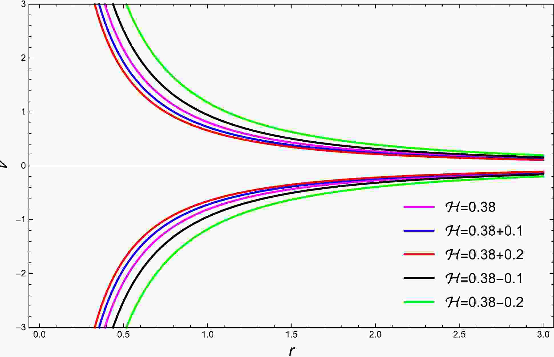
$ {\cal{H}} $ is${\cal{H}}_{\rm min}=r^{-2} (\nu +r)^{-2}$ . Physical flows are represented by the curves that lie between the two green curves in Fig. 1. Furthermore, the curves on the bottom half-plane with$ \nu < 0 $ represent the fluid accretion, and the curves on the top half-plane with$ \nu > 0 $ depict the outer flow of the fluid or the emission of particles.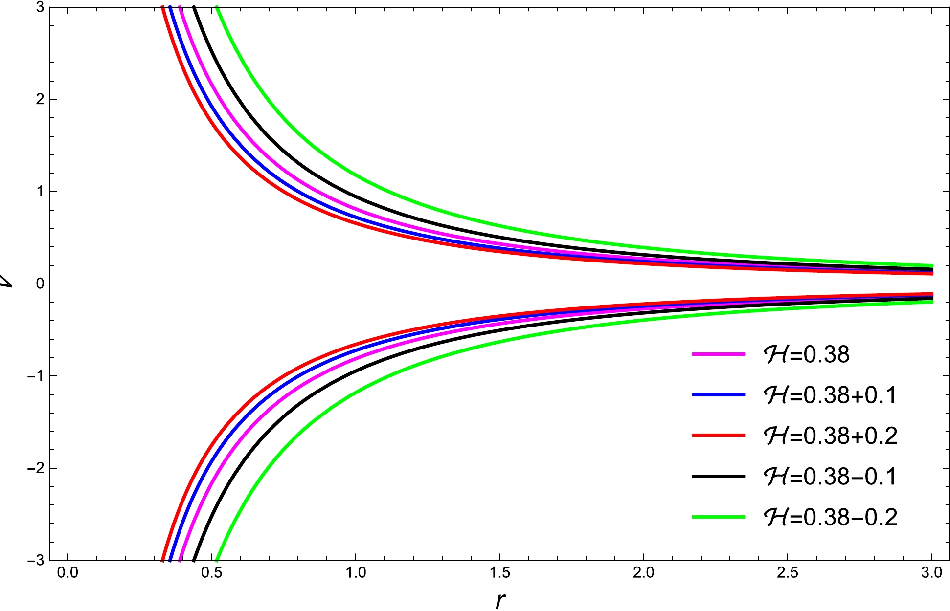
Figure 1. (color online) Profile of
$ {\cal{H}} $ (83) for the ultra-stiff fluid with BH parameters$ M=1 $ ,$ \alpha=0.1 $ , and$ \beta=0.16 $ . The magenta curve represents${\cal{H}}= {\cal{H}}_{\rm min}\simeq$ 0.38. The green and black curves refer to${\cal{H}} > {\cal{H}}_{\rm min}$ , whereas the blue and red curves represent the behavior for${\cal{H}} < {\cal{H}}_{\rm min}$ .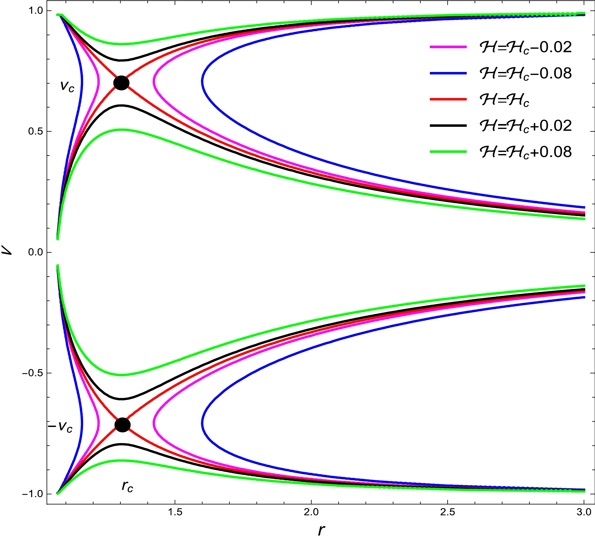
Figure 2. (color online) Plot of
$ {\cal{H}} $ (86) for ultra-relativistic fluid with the BH parameters$ M = 1 $ ,$ \alpha = 1.5 $ , and$ \beta = 1.5 $ . The critical points$ (r_{c},\nu_{c}) $ are shown by black dots. In Fig. 2, five plots are provided, with red, black, green, magenta, and blue corresponding to the specified Hamiltonian values${\cal{H}}={\cal{H}}_{c}\simeq $ $ 0.557752$ ,$ {\cal{H}}={\cal{H}}_{c}+0.02 $ ,$ {\cal{H}}={\cal{H}}_{c}+0.08 $ ,$ {\cal{H}}={\cal{H}}_{c}-0.08 $ , and$ {\cal{H}}={\cal{H}}_{c}- 0.02 $ , respectively. -
Now, using the EOS parameter
$k = 1/2$ , or$p = e /2$ , we study the ultra-relativistic fluid for which the isotropic pressure of the fluid exceeds its energy density. Ultimately, we achieve the Hamiltonian (82) for$k=\dfrac{1}{2}$ in the following form:$ {\cal{H}}(r,\nu)=\frac{\left(1-\dfrac{2 M}{r}+\dfrac{\alpha M}{r^2}+\dfrac{(\alpha M)\ln\Big(\dfrac{r}{\beta }\Big)}{r^2}\right)^{\frac{1}{2}}}{(1-\nu^{2})^{\frac{1}{2}}\nu r^{2}}, $

(86) and the system expressed via (72) and (73) has the subsequent structure:
$\begin{aligned}[b] \dot{r}=&\frac{\sqrt{\dfrac{\alpha M+\alpha M \ln\Big(\dfrac{r}{\beta }\Big)-2 M r+r^2}{r^2}}}{(1-\nu ^2)^{3/2} r^2}\\&-\frac{\sqrt{\dfrac{\alpha M+\alpha M \ln\Big(\dfrac{r}{\beta }\Big)-2 M r+r^2}{r^2}}}{\nu ^2 \sqrt{1-\nu ^2} r^2}, \end{aligned}$

(87) $\begin{aligned}[b] \dot{\nu}=&-\left(\frac{\dfrac{\dfrac{\alpha M}{r}-2 M+2 r}{r^2}-\dfrac{2(\alpha M+\alpha M \ln\Big(\dfrac{r}{\beta }\Big)-2 M r+r^2)}{r^3}}{2 \nu \sqrt{1-\nu ^2} r^2 \sqrt{\dfrac{\alpha M+\alpha M \ln\Big(\dfrac{r}{\beta }\Big)-2 M r+r^2}{r^2}}}\right.\\&\left.-\dfrac{2 \sqrt{\dfrac{\alpha M+\alpha M \ln\Big(\dfrac{r}{\beta }\Big)-2 M r+r^2}{r^2}}}{\nu \sqrt{1-\nu ^2} r^3}\right).\end{aligned} $

(88) Furthermore, using Eqs. (87) and (88), we find the critical points of the dynamical system for ultra-relativistic fluid. By assuming the BH parameters
$ M = 1 $ ,$ \alpha = 1.5 $ , and$ \beta = 1.5 $ , we determine that the physical critical points$ (r_{c}, \pm\nu_{c}) $ are$ (1.303808, -0.7071067) $ and$(1.303808, 0.7071067)$ , which represent the outer flow and accretion of the fluid, respectively. This critical Hamiltonian,$ {\cal{H}}_{c}=0.557752 $ , is obtained by inserting these critical points into Eq. (86). Table 1 contains a list of the critical points$ r_c $ ,$ \nu_c $ , and$ {\cal{H}}_{c} $ for different values of the BH parameter. Several curves depict the behavior of the ultra-relativistic fluid with the BH parameters$ M = 1 $ ,$ \alpha = 1.5 $ , and$ \beta= 1.5 $ in Fig. 2. In the dynamics of ultra-relativistic fluid, the saddle points$ (r_{c}, \pm\nu_{c}) $ are indicated in Fig. 2. As shown in Fig. 2, the green (with$ {\cal{H}}={\cal{H}}_{c}+0.08 $ branches) and black curves (with$ {\cal{H}}= {\cal{H}}_{c}+0.02 $ branches) represent purely supersonic outer flow ($ \nu>\nu_{c} $ branches), supersonic accretion$ (\nu<-\nu_{c}) $ , or purely subsonic accretion followed by subsonic outer flow$ (-\nu_{c}<\nu<\nu_{c}) $ . The magenta (with$ {\cal{H}}={\cal{H}}_{c} $ -0.08 branches) and blue curves (with$ {\cal{H}}={\cal{H}}_{c}-0.02 $ branches) indicate no physical behavior.$\alpha=1.5$ 

$ \beta=1.5$ 

β $ r_{c}$ 

$ \nu_{c}$ 

$ {\cal{H}}_{c}$ 

α $ r_{c}$ 

$ \nu_{c}$ 

$ {\cal{H}}_{c}$ 

1.1 0.90919 0.7071 1.25519 1.1 1.57581 0.7071 0.356241 1.2 1.02015 0.7071 0.95472 1.2 1.5 0.7071 0.397523 1.3 1.12339 0.7071 0.767776 1.3 1.429009 0.7071 0.444709 1.4 1.2179 0.7071 0.644097 1.4 1.36349 0.7071 0.498093 1.5 1.303808 0.7071 0.557752 1.5 1.303808 0.7071 0.557752 Table 1. Values of
$\nu_{c}$ ,$r_{c}$ , and$ {\cal{H}}_{c}$ at critical points with several values of BH parameters for ultra-relativistic fluid.The red arcs in Fig. 2 depict an interesting solution and demonstrate transonic behavior outward to the BH horizon. There are curves for
$ \nu<0 $ that intersect the sonic point$ (r_{c}, \nu_{c}) $ . One solution originates at spatial infinity with subsonic flow and proceeds to supersonic flow after exceeding the sonic point. This solution is related to the standard non-relativistic Bondi accretion, as described in . It is difficult to identify such behavior because according to Ref. , the alternative solution that tends to spatial infinity with supersonic flow but changes to subsonic after reaching the sonic point is unstable. There are two possibilities: if$ \nu> 0 $ or$ \nu<0 $ . If$ \nu> 0 $ , the transonic solution of the stellar wind, starting at the horizon with supersonic flow and transferring to subsonic flow after crossing the sonic point, is one solution for non-relativistic accretion that is described in. The other solution corresponds to the case$ \nu<0 $ , which is unstable and difficult to achieve. In general, different Hamiltonian values correlate with distinct dynamical system initial states. At the sonic point, the Hamiltonian of the transonic solution of the ultra-relativistic fluid can be evaluated. Because its values are different from those of the transonic one, the Hamiltonian is unable to present any transonic solutions to the flow. The magenta curve, for instance, shows fluid subcritical flow because it cannot reach the critical point. The nearest point this type of fluid is able to reach before rebounding or turning around infinity is the turning point, which exists physically for the solutions. Similar reasoning applies to the blue curves. Supercritical flows are shown by the green and black curves. Fluids move faster than the permitted critical value, even when they do not reach the critical points. Eventually, these particles reach the BH horizon. It is also important to note that other fluids, including radiation, sub-relativistic, and polytropic fluids, are subject to the same examination. -
Here, the state parameter value for radiation fluid is
$ k = \dfrac{1}{3} $ , and we obtain the Hamiltonian in the following form:$ {\cal{H}}(r,\nu)=\dfrac{\left(\dfrac{\alpha M+\alpha M \ln\Big(\dfrac{r}{\beta }\Big)-2 M r+r^2}{r^2}\right)^{2/3}}{\nu ^{2/3}(1-\nu ^2)^{2/3} r^{4/3}}, $

(89) The previous system of Eqs. (72) and (73) minimizes to
$ \begin{aligned}[b]\dot{\nu}=&- \left( \frac{2\left( \dfrac{\dfrac{\alpha M}{r}-2 M+2 r}{r^2}-\dfrac{2(\alpha M+\alpha M \ln (\dfrac{r}{\beta })-2 M r+r^2)}{r^3} \right)}{3 \nu ^{2/3}(1-\nu ^2)^{2/3} r^{4/3} \sqrt[3]{\dfrac{\alpha M+\alpha M \ln(\dfrac{r}{\beta })-2 M r+r^2}{r^2}}}\right. \end{aligned}$

$ \begin{aligned}[b]\left.-\dfrac{4\left(\dfrac{\alpha M+\alpha M \ln\Big(\dfrac{r}{\beta }\Big)-2 M r+r^2}{r^2}\right)^{2/3}}{3 \nu ^{2/3}(1-\nu ^2)^{2/3} r^{7/3}}\right), \end{aligned}$

(90) $ \begin{aligned}[b]\dot{r}=&\frac{4 \sqrt[3]{\nu }\left(\dfrac{\alpha M+\alpha M \ln\Big(\dfrac{r}{\beta }\Big)-2 M r+r^2}{r^2}\right)^{2/3}}{3(1-\nu ^2)^{5/3} r^{4/3}}\\&-\dfrac{2\left(\dfrac{\alpha M+\alpha M \ln \Big(\dfrac{r}{\beta }\Big)-2 M r+r^2}{r^2}\right)^{2/3}}{3 \nu ^{5/3}(1-\nu ^2)^{2/3} r^{4/3}}, \end{aligned}$

(91) From Eqs. (90) and (91), we can determine the critical points (
$ r_{c} $ ,$ \nu_{c} $ ), and then by inserting these points into Eq. (89), we obtain the critical Hamiltonian for radiation fluid. The critical values$ r_{c} $ ,$ \nu_{c} $ , and$ {\cal{H}}_{c} $ are given in Table 2.$\alpha=1.5$ 

$ \beta=1.5$ 

β $ r_{c}$ 

$ \nu_{c}$ 

$ {\cal{H}}_{c}$ 

α $ r_{c}$ 

$ \nu_{c}$ 

$ {\cal{H}}_{c}$ 

1.1 1.01804 0.57735027 0.952249 1.1 1.8585 0.57735027 0.379317 1.2 1.1527138 0.57735027 0.774299 1.2 1.75934 0.57735027 0.40996 1.3 1.27901 0.57735027 0.660915 1.3 1.66576 0.57735027 0.44493 1.4 1.39485 0.57735027 0.58408 1.4 1.57902 0.57735027 0.484581 1.5 1.5 0.57735027 0.529134 1.5 1.5 0.57735027 0.557752 Table 2. Values of
$\nu_{c}$ ,$r_{c}$ , and$ {\cal{H}}_{c}$ at critical points with various values of BH parameters for the radiation fluid.In Fig. 3, several curves illustrate the physical behavior of radiation fluid with the BH parameters
$ M = 1 $ ,$ \alpha = 1 $ ,$ \alpha = 1.5 $ , and$ \beta = 1.5 $ . The red curve corresponds to$ {\cal{H}}={\cal{H}}_{c} $ . The green and black curves correspond to$ {\cal{H}}>{\cal{H}}_{c} $ , whereas the blue and magenta curves correspond to$ {\cal{H}}<{\cal{H}}_{c} $ . Figure 3 shows the three primary types of fluid motion. For$ \nu > \nu_{c} $ , the red and green curves demonstrate supersonic outflows. These curves represent supersonic accretion for$ \nu <-\nu_{c} $ . The curves displayed for$ -\nu <\nu_{c}< \nu $ exhibit only subsonic accretion along with subsonic flow out with vanishing speed near the horizon. Non-physical behavior is illustrated by the magenta and black curves.
Figure 3. (color online) Contour plot
$ {\cal{H}} $ (89) of radiation fluid with the BH parameters$ M = 1 $ ,$ \alpha = 1.5 $ , and$ \beta = 1.5 $ . The critical points$ (r_{c},\pm\nu_{c}) $ are indicated by black dots. In Fig. 3, five plots are provided, with red, black, green, magenta, and blue corresponding to the specified Hamiltonian values${\cal{H}}={\cal{H}}_{c}\simeq $ $ 0.5291336$ ,$ {\cal{H}}={\cal{H}}_{c}+0.02 $ ,$ {\cal{H}}={\cal{H}}_{c}+0.08 $ ,$ {\cal{H}}={\cal{H}}_{c}-0.02 $ , and$ {\cal{H}}={\cal{H}}_{c}- 0.08 $ -
The energy density is greater than the isotropic pressure, and according to the EOS for a sub-relativistic fluid, we have
$ p = e/4 $ . The Hamiltonian (82) in this scenario is$ {\cal{H}}(r,\nu)=\frac{\left(\dfrac{\alpha M+\alpha M \ln\Big(\dfrac{r}{\beta }\Big)-2 M r+r^2}{r^2}\right)^{3/4}}{\sqrt{\nu }(1-\nu ^2)^{3/4} r}, $

(92) and the two-dimensional dynamical system expressed via (72) and (73) becomes
$\begin{aligned}[b] \dot{\nu}=&- \left( \frac{3\left( \dfrac{\dfrac{\alpha M}{r}-2 M+2 r}{r^2}-\dfrac{2(\alpha M+\alpha M \ln (\dfrac{r}{\beta })-2 M r+r^2)}{r^3} \right)}{4 \sqrt{\nu }(1-\nu ^2)^{3/4} r \sqrt[4]{\dfrac{\alpha M+\alpha M \ln\Big(\dfrac{r}{\beta }\Big)-2 M r+r^2}{r^2}}}\right.\\&\left.-\dfrac{\left(\dfrac{\alpha M+\alpha M \ln\Big(\dfrac{r}{\beta }\Big)-2 M r+r^2}{r^2}\right)^{3/4}}{\sqrt{\nu }(1-\nu ^2)^{3/4} r^2}\right).\\[-20pt]\end{aligned} $

(93) $ \begin{aligned}[b]\dot{r}=&\frac{3 \sqrt{\nu }\left(\dfrac{\alpha M+\alpha M \ln\Big(\dfrac{r}{\beta }\Big)-2 M r+r^2}{r^2}\right)^{3/4}}{2(1-\nu ^2)^{7/4} r}\\&-\dfrac{\left(\dfrac{\alpha M+\alpha M \ln\Big(\dfrac{r}{\beta }\Big)-2 M r+r^2}{r^2}\right)^{3/4}}{2 \nu ^{3/2}(1-\nu ^2)^{3/4} r},\end{aligned} $

(94) Table 3 displays the critical values
$ r_{c} $ ,$ \omega_{c} $ , and$ {\cal{H}}_{c} $ for the sub-relativistic fluid, and Fig. 4 displays the sub-relativistic fluid phase space characteristics. The motion of the sub-relativistic fluid with$ (k =\dfrac{1}{4}) $ is equivalent to that of the radiation fluid with$ (k=\dfrac{1}{3}) $ and the ultra-relativistic fluid with$ (k=\dfrac{1}{2}) $ , as observed in Fig. 4. For$ \nu > \nu_{c} $ , the black and green curves show supersonic accretion, whereas for$ \nu<- \nu_{c} $ , they exhibit only supersonic outer flows. Additionally, when$ -\nu_{c}< \nu <\nu_{c} $ , these curves show subsonic flows. In Fig. 4, the red curves show the transonic outer flow solution for$ \nu > 0 $ and the spherical accretion for$ \nu< 0 $ , which are incredibly interesting. The magenta and blue curves, similar to the case of the radiation fluid, reveal that the ultra-relativistic fluid exhibits non-physical behavior in this case.$\alpha=1.5$ 

$ \beta=1.5$ 

β $ r_{c}$ 

$ \nu_{c}$ 

$ {\cal{H}}_{c}$ 

α $ r_{c}$ 

$ \nu_{c}$ 

$ {\cal{H}}_{c}$ 

1.1 1.10713 0.5 0.834557 1.1 2.14397 0.5 0.405427 1.2 1.26724 0.5 0.705269 1.2 2.01837 0.5 0.429966 1.3 1.41874 0.5 0.622867 1.3 1.89838 0.5 0.458071 1.4 1.55782 0.5 0.566852 1.4 1.7862 0.5 0.455547 1.5 1.683639 0.5 0.526559 1.5 1.683639 0.5 0.526559 Table 3. Values of
$\nu_{c}$ ,$r_{c}$ , and$ {\cal{H}}_{c}$ at critical points with different values of BH parameters for ultra-relativistic fluid.
Figure 4. (color online) Contour plot of
$ {\cal{H}} $ (89) for sub-relativistic fluid with the BH parameters$ M = 1 $ ,$ \alpha = 1.5 $ , and$ \beta = 1.5 $ . The critical points$ (r_{c},\pm\nu_{c}) $ are indicated by black dots. In Fig. 4, five plots are provided, with red, black, green, magenta, and blue corresponding to the following Hamiltonian values:$ {\cal{H}}={\cal{H}}_{c}\simeq 0.526558 $ ,$ {\cal{H}}={\cal{H}}_{c}+0.2 $ ,$ {\cal{H}}={\cal{H}}_{c}+0.4 $ ,$ {\cal{H}}={\cal{H}}_{c}-0.04 $ , and$ {\cal{H}}={\cal{H}}_{c}- 0.08 $ . -
For polytropic test fluid, the EOS is
$ p=G(n)=Kn^{\gamma}, $

(95) where K and γ are assumed to be constants. To work with ordinary objects, the constraint
$ \gamma>1 $ is often utilized. For the specific enthalpy [12], we obtain the following equation:$ h=M_{1}+\frac{K\gamma n^{\gamma-1}}{\gamma-1}, $

(96) where the baryonic mass
$ M_{1} $ is the integration constant. The speed of sound is$ a^{2}=\frac{(\gamma-1)Y}{M_{1}(\gamma-1)+Y}\,\,\,\,\,\,\ Y=K\gamma n^{\gamma-1}. $

(97) Eqs. (76) and (97) give us
$\begin{aligned}[b]\\[-15pt] h=M_{1}\left(1+Z\left(\frac{1-\nu^{2}}{r ^{4}\nu^{2}\left(1-\dfrac{2 M}{r}+\dfrac{\alpha M}{r^2}+\dfrac{(\alpha M)\ln\Big(\dfrac{r}{\beta }\Big)}{r^2}+u^{2}\right)}\right)^{\textstyle\frac{\gamma-1}{2}}\right) ,\end{aligned} $ 
(98) where
$\begin{aligned}[b] Z=\frac{K\gamma n^{\gamma-1}_{c}}{M_{1}(\gamma-1)}\Big(-\frac{1}{4} M r_c^2\Big(\alpha +2 \alpha \ln\Big(\frac{r_c}{\beta }\Big)-2 r_c\Big)\Big)^{\textstyle\frac{\gamma-1}{2}}= {\rm constant} >0,\end{aligned} $

(99) where Z is a positive constant. Utilizing Eqs. (98) and (70), we determine
$\begin{aligned}[b] {\cal{H}}=\frac{\left(1-\dfrac{2 M}{r}+\dfrac{\alpha M}{r^2}+\dfrac{(\alpha M)\ln\Big(\dfrac{r}{\beta }\Big)}{r^2}\right)}{1-\nu^{2}}\left[1+Z\left(\frac{1-\nu^{2}}{r ^{4}\nu^{2}\left(1-\dfrac{2 M}{r}+\dfrac{\alpha M}{r^2}+\dfrac{(\alpha M)\ln\Big(\dfrac{r}{\beta }\Big)}{r^2}\right)}\right)^{\textstyle\frac{\gamma-1}{2}}\right]^{2},\end{aligned} $

(100) where
$ M^{2} $ disappears within the re-definition of$ \bar{t}, {\cal{H}} $ . Because the Hamiltonian is constant on the solution curve, no global solutions are possible. Considering the procedure given in [12, 56], we can obtain$ a_{c}^{2}= Z(\gamma-1-\omega_{c}^{2})\left(\frac{1-\nu _c^2}{\nu _c^2 r_c^2(\alpha M(\ln (\dfrac{r_c}{\beta } )+1)-2 M r_c+r_c^2)}\right)^{\frac{\gamma-1}{2}}, $

(101) $ \omega_{c}^{2}=-\frac{M(\alpha +2 \alpha \ln\Big(\dfrac{r_c}{\beta }\Big)-2 r_c)}{\alpha M(2 \ln \Big(\dfrac{r_c}{\beta }\Big)+3)-6 M r_c+4 r_c^2}. $

(102) As observed from Fig. 5, the solution curve does not cross the r-axis at point
$ (r_{h},0) $ because the Hamiltonian (100) diverges there. Moreover, the numerical solution of the Hamiltonian (100) is shown, which demonstrates that the motion of a polytropic fluid has similarities to those of isothermal, radiation, and sub-relativistic fluids, which are given in the previous sub-sections.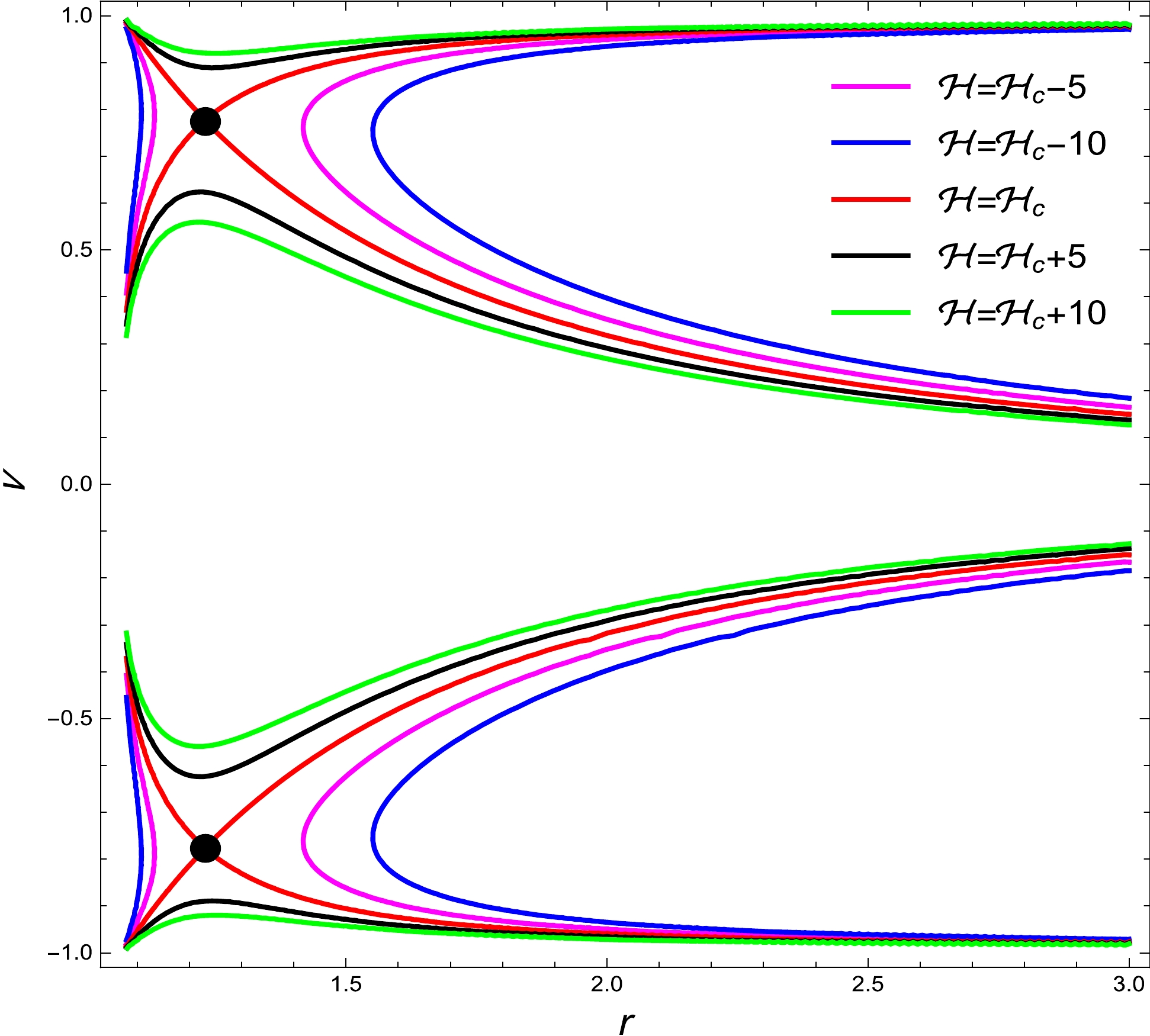
Figure 5. (color online) Contour plot
$ {\cal{H}} $ (100) for the polytropic fluid with the BH parameters$ M = 1 $ ,$ \alpha = 1.5 $ , and$ \beta = 1.5 $ . The sonic critical points$ (r_{c},\pm\nu_{c}) $ are indicated by black dots. In Fig. 5, five plots are provided, with red, black, green, magenta, and blue corresponding to the Hamiltonian values$ {\cal{H}}={\cal{H}}_{c}=69.28 $ ,$ {\cal{H}}={\cal{H}}_{c}+5 $ ,$ {\cal{H}}={\cal{H}}_{c}+10 $ ,$ {\cal{H}}={\cal{H}}_{c}-10 $ , and$ {\cal{H}}={\cal{H}}_{c}- 5 $ , respectively. -
In this section, we obtain the mass accretion rate of fluid onto the static and spherically symmetric hairy BH using the GD framework. We know that as matter accretes in the vicinity of a compact object, its mass varies over time. As matter accumulates around the compact object, its mass varies gradually. The provided relationship,
$\dot{M}=-\int T^{1}_{0}{\rm d}S$ , where${\rm d}S=\sqrt{-g}{\rm d}\theta {\rm d}\phi$ , can be employed to determine the BH mass rate change over time. We can utilize the typical formula provided in [9] to compute the mass accretion rate as follows:$ \dot{M}=4\pi LM_{2}^{2}(e+p) , $

(103) and from Eqs. (43) and (44), we have
$ r^{2}uh \sqrt{1-\frac{2 M}{r}+\frac{\alpha M}{r^2}+\frac{(\alpha M)\ln\Big(\dfrac{r}{\beta }\Big)}{r^2}+u^{2}}=K_{0}. $

(104) The specified expression can be calculated using the relativistic flux equation under
$ r^{2}u^{r} {\rm e}^{\textstyle\int^{e}_{e_{\infty}}\frac{{\rm d}e^{'}}{e^{'}+p(e^{'})}}=-K_{1}, $

(105) where
$ K_{1} $ indicates the constant of integration. By substituting$ p=ke $ into Eq. (105), we acquire$ e=\Big(\frac{K_{1}}{r^{2}u}\Big)^{k+1}. $

(106) From Eqs. (80), (106) and (104), we get
$ u^{2} - \frac{K_{0}^{2}K_{1}^{-2(k+1)}}{(k+1)^{2}}r^{4k}(-u)^{2k} + \Big(1 - \frac{2 M}{r} + \frac{\alpha M}{r^2} + \frac{(\alpha M)\ln\Big(\dfrac{r}{\beta }\Big)}{r^2}\Big) = 0. $

(107) We can analytically compute
$ u^{r} $ to consider various values of k by evaluating the above expression. For$ k=1 $ , Eq. (107) gives us$ u=\pm 2K_{1}\sqrt{\frac{1-\dfrac{2 M}{r}+\dfrac{\alpha M}{r^2}+\dfrac{(\alpha M)\ln\Big(\dfrac{r}{\beta }\Big)}{r^2}}{K_{0}^{2}r^{4}-4K_{1}^{4}}}, $

(108) and using Eqs. (108), (106), and (103), it yields
$ \dot{M}=2\pi \frac{K_{0}^{2}r^{4}-4K_{1}^{4}}{r^{4}K_{1}\left(1-\dfrac{2 M}{r}+\dfrac{\alpha M}{r^2}+\dfrac{(\alpha M)\ln\Big(\dfrac{r}{\beta }\Big)}{r^2}\right)} , $

(109) where
$ \dot{M} $ is the mass accretion rate for the static and spherically symmetric hairy BH in the framework of GD with constants$ K_{0} $ and$ K_{1} $ . Furthermore, if we set$ k=1/2 $ , we can acquire the mass accretion rate for ultra-relativistic fluid presented below.$ \dot{M_{\rm acc}}=162 \pi\left(\frac{K_1^4}{r^2 \left(K_1^3 \sqrt{\dfrac{4 K^4 r^4}{K_1^6}-\dfrac{81 \left(\alpha M+\alpha M \ln \left(\dfrac{r}{\beta }\right)-2 M r+r^2\right)}{r^2}}-2 K^2 r^2\right)}\right)^{3/2}. $ 
(110) The graph of the mass accretion rate is depicted in Fig. 6. From Fig. 6, we find that, as the values of the BH parameters increase, the mass accretion rate decreases.
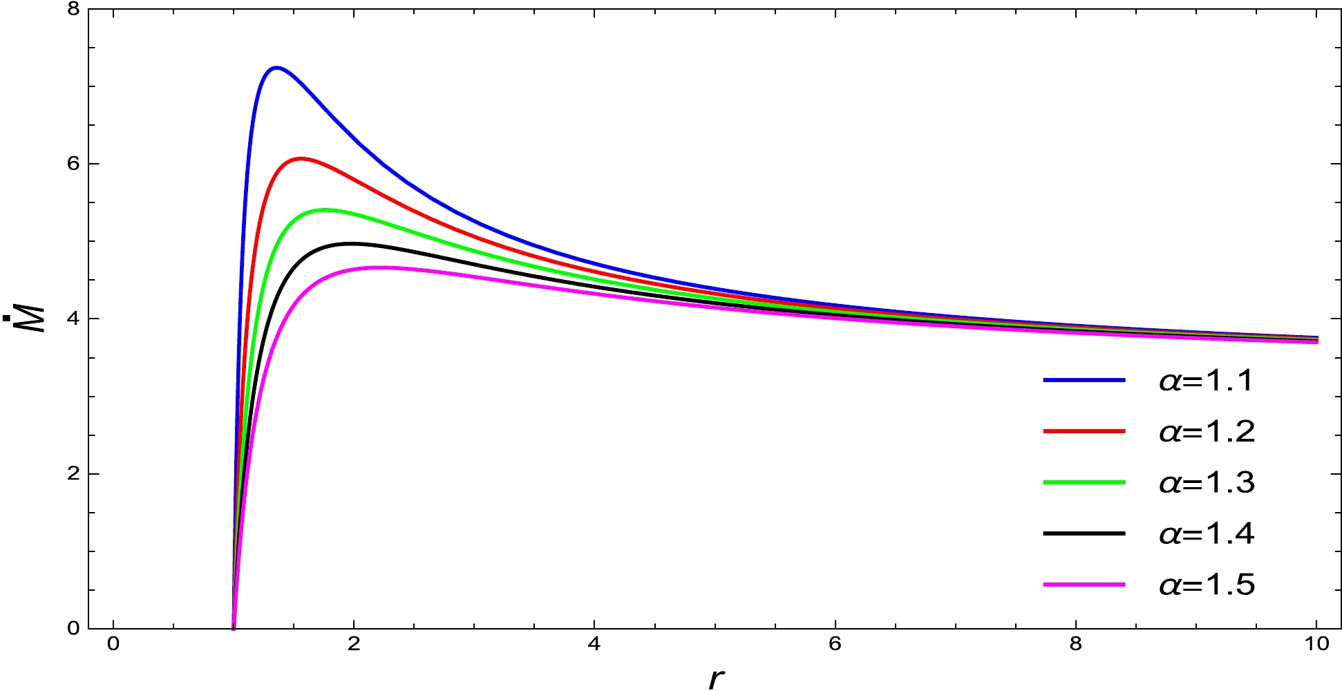
Figure 6. (color online)
$\dot{M}_{\rm acc}$ versus r for$ M = 1 $ ,$ \beta = 1.5 $ , and various values of α. As α increases, the mass accretion rate decreases. -
This study investigates the spherical accretion flow of a perfect fluid around a static and spherically symmetric hairy BH in the framework of GD. Applying energy and particle conservation equations, we provide two fundamental expressions for analyzing accretion phenomena. Then, using these basic formulations, we investigate the accretion flow of various perfect fluids, such as ultra-stiff, ultra-relativistic, radiation, sub-relativistic, and perfect isothermal fluids. Figures 1, 2, 3, 4, and 5 depict the motion of a variety of fluids around the static and spherically symmetric hairy BH in the framework of GD. It is important to note that the sonic point does not exist for ultra-stiff fluids. We determine the critical values for ultra-relativistic, radiation, and sub-relativistic fluids, which are listed in Tables 1, 2, and 3. We examine the physical characteristics of matter, including ultra-stiff, ultra-relativistic, radiation, and sub-relativistic fluids, with the EOS, which permits us to determine the nature of BHs. We discover that the various forms of accreting fluid exhibit distinct accretion behavior, such as subsonic, supersonic, and transonic flow, according to the EOS and model parameters. We observe that supersonic accretion followed by subsonic accretion ends within the horizon of the BH. This means that the fluid flow throughout the accretion of matter onto hairy BHs within the framework of GD is neither supersonic nor transonic within the vicinity of the horizon. The outer flow is unstable as it follows a subsonic path that passes through the critical point
$ (r_{c},\nu_{c}) $ and then becomes subsonic.Moreover, the mass accretion rate of BHs is found for ultra-stiff fluid (
$ k = 1 $ ) and ultra-relativistic fluid ($ k = 1/2 $ ). The effect of the BH parameters on the spherical mass accretion rate of perfect fluid onto massive objects is also graphically examined. It is obvious from Fig. 6 that the mass accretion rate would attain its highest value for a BH with a small radius and then decline to a constant value for BHs with larger radii. Moreover, we observe an inverse relationship between mass accretion and the BH parameters. The results described in the preceding section indicate that the mass accretion rate is dependent on the EOS parameter, and this dependence is only discernible when the EOS parameter value is small. Because Eq. (107) becomes highly non-linear with respect to u, it is impossible to identify an explicit form of$ \dot{M} $ for further values of the state parameter.
Accretion around a hairy black hole in the framework of gravitational decoupling theory
- Received Date: 2023-08-22
- Available Online: 2023-12-15
Abstract: We investigate astrophysical accretion onto a static and spherically symmetric hairy black hole within the framework of gravitational decoupling. To achieve this goal, we examine the accretion procedure for several types of perfect fluids, including polytropic fluid and ultra-stiff, ultra-relativistic, radiation, and sub-relativistic isothermal fluids. Moreover, we determine the critical or sonic points for numerous fluid forms that are accreting onto the black hole by utilizing the Hamiltonian dynamical approach. Additionally, the closed form of the solutions are presented for a number of fluids, which are represented in phase diagram curves. We estimate the mass accretion rate of a static and spherically symmetric hairy black hole within the framework of gravitational decoupling. These findings are helpful in constraining the parameters of black holes while physical matter accretes onto the black holes.


 DownLoad: