Nuclear mass predictions based on a deep neural network and finite-range droplet model (2012)

Nuclear mass is one of the most fundamental nuclear properties [1, 2]. It not only represents the static properties of nuclei but also determines the reaction energies in different nuclear processes, such as β decay, neutron capture, and fission [3]. All these processes play important roles in the origin of elements and the abundance of elements in the universe [3−5].

Currently, there are approximately 2500 nuclei with experimental masses. These nuclei are estimated to be only 27.8% of around 9000 theoretically estimated bounded nuclei [2, 6]. To gain a better understanding of nuclear mass for all nuclei, theoretical mass models are required. There are several theoretical models for mass prediction. Some of them are microscopic models, such as Hartree–Fock–Bogoliubov (HFB) [7, 8] and relativistic mean-field (RMF) mass models [9], whereas others are macroscopic-microscopic models, such as the finite-range droplet [6] and Weizsäcker–Skyrme (WS) models [10]. These theoretical models give a root-mean-square (RMS) deviation of 0.3 to 2.3 MeV between the theoretical and experimental masses [11]. To reduce RMS deviation, which is critical for a better description of final element abundance [3, 4], a machine learning model can be developed.

Neural networks, a type of algorithm in machine learning, have been widely used in different research fields [12−14]. Several recent studies have proven that neural networks are able to improve the accuracy of models for several different nuclear properties, such as the β-decay half-lives [15, 16], neutron capture rate [17], nuclear charge radii [18], and ground-state and excited energies [19].

Neural networks have also been used in nuclear mass prediction in several previous studies [11,20−22]. For example, artificial neural networks (ANNs) [21], support vector machines (SVMs) [23], Bayesian neural networks (BNNs) [11], Bayesian machine learning (BML) [22], Gaussian process [24], light gradient-boosting machine (LightGBM) [25], the radial basis function (RBF/RBF-oe) [26], kernel ridge regression (KRR/KRR-oe) [27], and naive Bayesian probability classifier (NBP) [28] have been used in mass prediction. The ANN algorithm [21] was used to determine the effects of different numbers of hidden layers. The effects of different numbers of inputs were investigated using ANNs [21] and BNNs [11]. An SVM [23] was used to investigate the effects of the training, validation, and test set ratio. The BML model [22] was used with nine different BNNs in total to predict the nuclear mass. The Gaussian process [24] was found to reduce the RMS deviation of the nuclear mass to less than $ 200 $ keV and help flatten out the discrepancies of nuclear mass in exotic regions. The LightGBM model [25] including $ 10 $ input features was used to show the effects of different ratios of training and test sets. The RBF/RBF-oe approach [26] showed the correlation between the target nuclei and their surrounding nuclei, the KRR/KRR-oe approach [27] has been used on the odd-even effects of the nuclei, and the NBP model [28] was used to calculate the nuclear mass after classifying the residuals of the nuclei into different groups.

The machine learning methods listed above have different advantages. The Bayesian methods, including BNNs [11], BML [22], and the NBP [28], include probability distributions in the parameters; thus, they can avoid the over-fitting problem and provide a probability distribution for the mass prediction in unknown regions. The Gaussian process [24] is similar to the previous methods; however, it includes probability distributions over the sample functions and also gives a probability distribution for the mass prediction. SVMs [23] can determine the number of hidden units automatically so that the number of hyperparameters can be reduced. The LightGBM [25] can accelerate the training process, reduce the computational time, and allow us to check the importance of different inputs of the model toward the outputs. The RBF/RBF-oe approach [26] can predict the mass based on the distance from the target nuclei to the training set. The KRR/KRR-oe approach [27] can identify the limit of the extrapolation distance of the model automatically so that the worst nuclear mass predictions far from the experimental results can be avoided.

Meanwhile, each neural network in these studies included several types of hyperparameters, such as the number of hidden units, choice of activation functions, initializers, and learning rates [16, 29]. These hyperparameters play very important roles in both the training process and final performance of the neural network. In other words, it is essential to investigate such hyperparameters in an explicit and systematic way.

In this study, a deep neural network (DNN) is used to construct a mass model that improves upon the current finite-range droplet model [6]. Different hyperparameters are particularly investigated to achieve a better neural network model. Moreover, several different sets of hyperparameters are used together to predict the nuclear masses and provide the uncertainty of the result.

The details of the neural network used in this study are given in Sec. II. The results of the nuclear mass neural network model and its performance are discussed in Sec. III. Finally, a summary is presented in Sec. IV. All the hyperparameters adjusted in this study are given in Appendices A, B, C, and D.

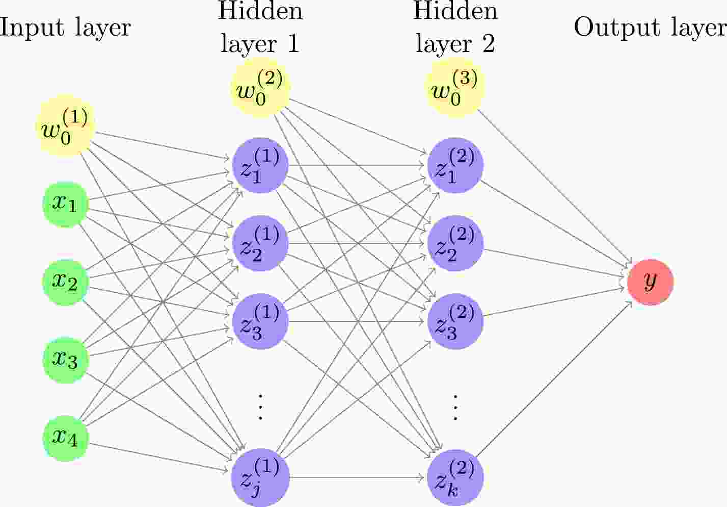
In this study, a DNN consisting of an input layer, two hidden layers, and an output layer is used, as shown in Fig. 1. The relationships between the input, hidden, and output layers are as follows:

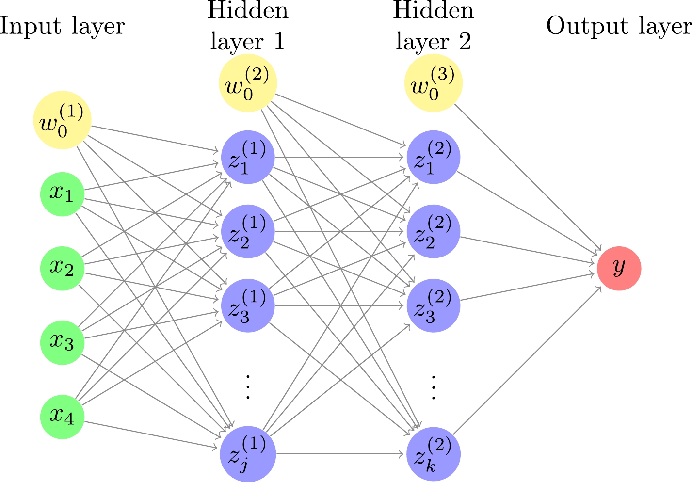
Figure 1.  (color online) Deep neural network with four inputs, two hidden layers, and one output. The number of hidden units is j and k for the first and second hidden layers, respectively. For each of the input and hidden layers, there is a bias term shown by a yellow circle.

where $ x_i $, $ z^{(1)}_j $, $ z^{(2)}_k $, and $ y_l $ are the inputs, the hidden units in the first hidden layer, the hidden units in the second hidden layer, and the output of the model, respectively. Here, $ {\boldsymbol{w}}=\{w^{(1)}_{ji},w^{(2)}_{kj},w^{(3)}_{lk},w^{(1)}_{j0},w^{(2)}_{k0}, w^{(3)}_{l0}\} $ are the parameters of the model, S is the sigmoid function [30]

and σ is the softmax function [30]

which makes the sum of $ z^{(2)}_k $ in the second hidden layer equal to $ 1 $. The hyperbolic tangent [30] has also been used as the activation function for the model,

The key reasons for choosing the sigmoid and softmax functions as the activation functions can be found in Appendix A.

The inputs of the neural network are given by $ {\boldsymbol{x}}=\{Z,N,\delta,P\} $, that is, including the neutron number N and proton number Z, together with information about the nuclear pairing δ and shell effect P. In particular, the information about nuclear pairing is characterized by

and hence, $ \delta=1 $ for even-even nuclei, $ \delta=0 $ for odd-A nuclei, and $ \delta=-1 $ for odd-odd nuclei. The information about the shell effect is characterized by

where $ v_p,v_n $ are the difference between Z, N and the closest magic number ($ 2 $, $ 8 $, $ 20 $, $ 28 $, $ 50 $, $ 82 $, $ 126 $, or $ 184 $), respectively [31].

In this study, the finite-range droplet model (FRDM12) is used as the theoretical mass model [6]. FRDM12 is a macroscopic–microscopic model, which includes the finite-range liquid-drop model in Eq. (9) as the macroscopic model,

and the folded-Yukawa single-particle potential as the microscopic corrections [6]. FRDM12 has a relatively small RMS deviation between the experimental and theoretical masses when compared with other theoretical mass models. Its overall RMS deviation is 0.603 MeV, whereas the RMS deviation of the nuclear mass for the RMF model is 2.269 MeV [11]. Furthermore, the FRDM model has been used to develop different models for β-decay properties, such as the FRDM+QRPA model [3]. Therefore, the improved FRDM12 with the neural network model can be used to improve these β-decay models.

The aim of this study is to obtain the mass residuals between the theoretical FRDM12 mass $ M_{l,\rm{FRDM12}} $ [6] and the experimental mass $ M_{l,\rm{exp}} $ [2],

To achieve the target mass residuals from the neural network, different hyperparameters of the model must be adjusted. The mean-square-error,

is used as the loss function, with $ y_l $ and $ t_l $ obtained from Eqs. (3) and (10), respectively. The Adam algorithm [32] with a learning rate of 0.01 is used to adjust the parameters $ {\boldsymbol{w}} $to achieve a smaller loss function. The corresponding key reasons are shown in Appendix B. Each of the hidden layers consists of 22 hidden units and a bias (the key reasons are presented in Appendix C). Therefore, there are $ 639 $ parameters in $ {\boldsymbol{w}} $ for the model.

For the initial parameter $ {\boldsymbol{w}} $ before training, we use three different initializers: the standard normal initializer, Glorot normal initializer, and zeros initializer [33]. The standard normal initializer distributes the initial parameters from a standard normal distribution with a mean of $ 0 $ and a standard deviation of $ 1 $. The Glorot normal initializer distributes the initial parameters from a normal distribution with a mean of $ 0 $ and a standard deviation equaling $ \sqrt{{2}/(f_{\rm{in}}+f_{\rm{out}})} $. In the above equation, $ f_{\rm in} $ and $ f_{\rm out} $ are the numbers of input and output units of that layer, respectively [33]. The zeros initializer sets the initial parameters to zero [33]. In this study, the initial parameters $ {\boldsymbol{w}} $ before training are generated from the standard normal distribution for $ \{w^{(1)}_{ji}, w^{(2)}_{kj}\} $ and the Glorot normal distribution for $ \{w^{(1)}_{j0}, w^{(2)}_{k0}\} $ (the key reasons are presented in Appendix D).

The experimental data of this study are taken from the atomic mass evaluation of 2020 (AME2020) [2]. There are 2457 nuclei in total with $ Z,N \geq 8 $. They are randomly separated into a training set and validation set. 1966 nuclei (80%) are randomly selected for the training set, and the remaining 491 nuclei (20%) are in the validation set.

To achieve a neural network with less variance in the prediction of mass, $ 33 $ sets of hyperparameters with different regularizers and seed numbers are used for training. There are three different types of regularizers used in this study. The first type is without using any regularizer. The second type is the L2 regularizer, which includes an additional term in the loss function [34],

where λ is a hyperparameter controlling the rate of regularization. The third type is the orthogonal regularizer, which encourages the basis of the output space of the layer to be orthogonal to each other [34]. The hyperparameter λ is used to control the rate of regularization.

In the following calculations, 20000 epochs are run for each training, and the smallest RMS deviation between $ t_l $ and $ y_l $ of the validation set in different epochs is used to determine the performance of the set of hyperparameters. Only the sets of hyperparameters giving an RMS deviation smaller than 0.228 MeV for the validation set (a reduction in RMS deviation of over 60% compared with the FRDM12 prediction) are selected. The average prediction from the selected sets of hyperparameters is the model output y. Summing the model output y and theoretical FRDM12 mass $ M_{k,\rm{FRDM12}} $ will give us the model mass prediction for the nuclei.

Of the 33 sets of hyperparameters, seven sets have an RMS deviation reduction greater than 60%, as shown in Fig. 2. Different regularizers speed up or slow down the training of the model, compared with the model without a regularizer (panel (a)). Note that from the 33 sets of hyperparameters, three are without regularizers and only one of them has an RMS deviation reduction over 60%. For the 12 sets of hyperparameters using the orthogonal regularizers, four have an RMS deviation reduction over 60%. For the nine sets of hyperparameters using L1 or L2 regularizers, none and two have an RMS deviation reduction over 60%, respectively. This shows that the regularizers still have an effect on the model. Moreover, because the seed number will affect the random numbers generated during training and the initial values of the parameters, different seed numbers are tried for the model. As shown in Table 1, the RMS deviations have average reductions from 0.603 to 0.200 MeV and 0.232 MeV, having improvements of 66.8% and 61.5% for the training and validation sets, respectively. This shows that the neural network can improve the accuracy of the FRDM12 model after adjusting the hyperparameters.

Figure 2.  (color online) RMS deviations of the training and validation sets with different sets of hyperparameters. Only the seven sets of hyperparameters with a reduction in RMS deviation larger than 60% are selected as follows: (a) No regularizer, seed=3, (b) L2 regularizer, $ \lambda=0.00001 $, seed $ =1 $, (c) L2 regularizer, $ \lambda=0.00001 $, seed $ =2 $, (d) orthogonal regularizer, $ \lambda =0.1 $, seed $ =2 $, (e) orthogonal regularizer, $ \lambda=0.01 $, seed $ =1 $, (f) orthogonal regularizer, $ \lambda=0.001 $, seed $ =1 $, and (g) orthogonal regularizer, $ \lambda=0.001 $, seed $ =2 $. The blue and orange curves represent the RMS deviations of the training and validation sets, respectively. The arrow points to the lowest RMS deviation of the validation set within the 20000 epochs.

Hyperparameters	$ \sigma_{\rm training} $/MeV	$ \sigma_{\rm validation} $/MeV	$ \Delta\sigma_{\rm training} $ (%)	$ \Delta\sigma_{\rm validation} $ (%)
No regularizer, seed $ =3 $	$ 0.175 $	$ 0.228 $	$ 71.0 $	$ 62.2 $
L2 regularizer, $ \lambda=0.00001 $, seed $ =1 $	$ 0.204 $	$ 0.226 $	$ 66.2 $	$ 62.5 $
L2 regularizer, $ \lambda=0.00001 $, seed $ =2 $	$ 0.216 $	$ 0.235 $	$ 64.2 $	$ 61.0 $
Orthogonal regularizer, $ \lambda=0.1 $, seed $ =2 $	$ 0.212 $	$ 0.218 $	$ 64.8 $	$ 63.8 $
Orthogonal regularizer, $ \lambda=0.01 $, seed $ =1 $	$ 0.176 $	$ 0.238 $	$ 70.8 $	$ 60.5 $
Orthogonal regularizer, $ \lambda=0.001 $, seed $ =1 $	$ 0.219 $	$ 0.238 $	$ 63.7 $	$ 60.5 $
Orthogonal regularizer, $ \lambda=0.001 $, seed $ =2 $	$ 0.201 $	$ 0.238 $	$ 66.7 $	$ 60.5 $
Average of the above sets	$ 0.200 $	$ 0.232 $	$ 66.8 $	$ 61.5 $

Table 1.  RMS deviations of nuclear mass between the experimental data from AME2020 [2] and the model predictions. The original RMS deviation between experimental data and FRDM12 [6] is $ 0.603 $ MeV. For each set of hyperparameters, the RMS deviations for the training and validation sets are denoted by $ \sigma_{\rm training} $ and $ \sigma_{\rm validation} $, respectively. The last two columns show the reduction in RMS deviations from the original deviation $ 0.603 $ MeV to $ \sigma_{\rm training} $ and $ \sigma_{\rm validation} $, respectively.

For most of the isotopes and isotones, the neural network model can give good performance in mass prediction. For example, as shown in Fig. 3, the average of the seven selected sets of hyperparameters has a considerably better overall performance in the mass difference compared to the FRDM12 model for the Nd isotopes and $ N=66 $ isotones. These two isotopes and isotones are selected because they have enough nuclei that are not included in the training set, where the data in the training set are represented by the gray-hatched regions in Fig. 3. In general, the mass prediction in the training set is better than that in the validation set. For the regions far from the training set, such as $ N<68 $ for Nd isotopes and $ Z>59 $ for $ N=66 $ isotones, the mass difference is still within the mass uncertainty shown in the yellow-hatched regions; therefore, the neural network model still exhibits good performance in these regions. However, the error bar for the neural network model is larger in regions far from the training set, which indicates that the mass predictions for different sets of hyperparameters in these regions have large variations. Therefore, multiple sets of hyperparameters are selected, and averaging the prediction of the seven sets of hyperparameters can provide the uncertainty of nuclear mass prediction for different nuclei. The larger the error bar for the nuclei, the less confidence we have in the mass prediction.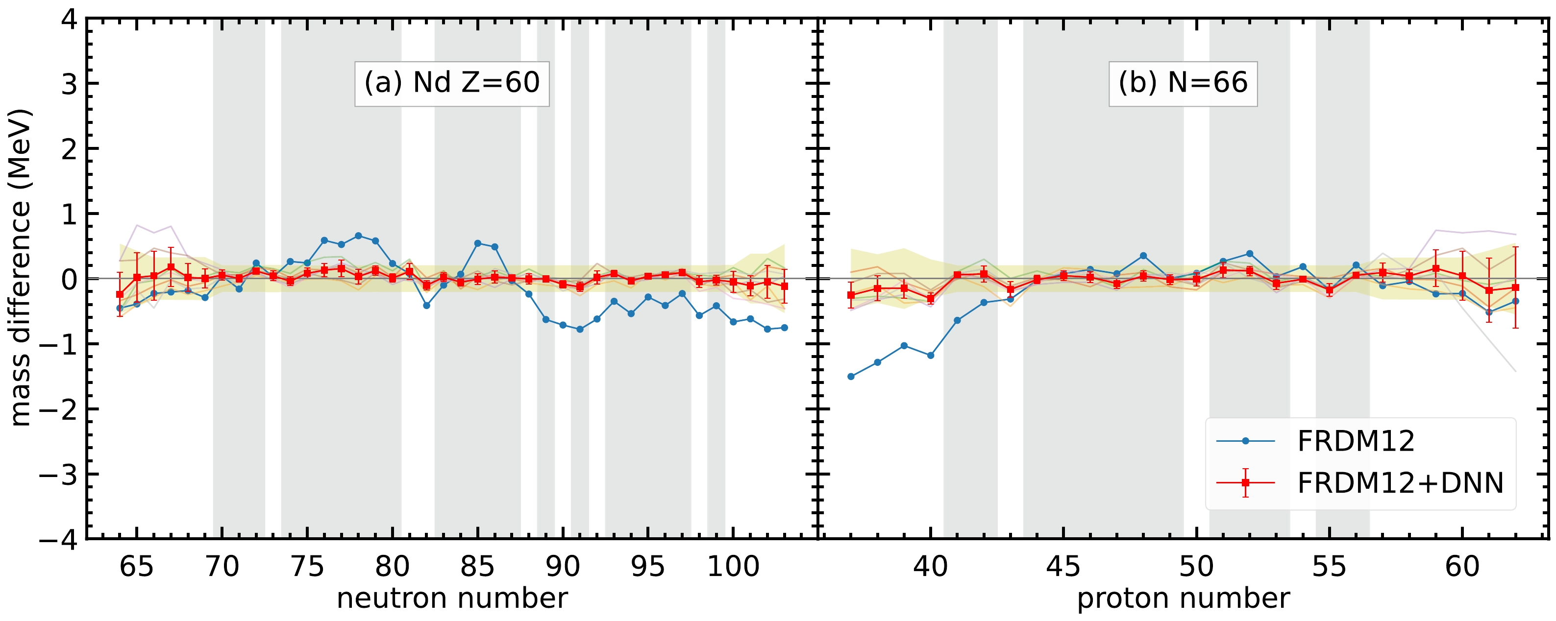

Figure 3.  (color online) Mass difference between the DNN mass data and experimental data, $t_k=M_{k,\rm DNN} - M_{k,\rm exp}$, for (a) Nd isotopes and (b) $ N=66 $ isotones. The blue curves represent the mass difference between the FRDM12 model and experimental data. The semi-transparent curves in the background represent the mass difference between the FRDM12+DNN mass model and experimental data with the seven sets of hyperparameters. The red curves with uncertainties represent the mass difference for the average of the FRDM12+DNN mass model. The error bars are calculated from the standard deviation of the mass difference from the $ 7 $ sets of hyperparameters. The gray-hatched regions represent the training set. The yellow-hatched regions represent the mass uncertainties by including the average RMS deviations of seven sets of hyperparameters together with the experimental uncertainties.

Furthermore, there are several nuclei whose the masses from the FRDM12 model are significantly different from the experimental data. For example, the mass difference can be up to $ 2.5 $ MeV. It is interesting to observe whether the neural network can significantly improve the mass predictions for these specific nuclei.

For Cr isotopes, shown in Fig. 4, FRDM12 cannot give a good mass prediction for the region $ N<22 $. In this region, the neural network model can still provide a better mass prediction compared with the FRDM12 model. Note that, the mass difference of the two nuclei $ N=17 $ and $ 18 $ is not within the yellow-hatched region. Although the mass prediction for the nucleus $ N=18 $ is not as good as that for other nuclei, the neural network model can improve the mass difference from $ -2.1 $ to $ -0.6 $ MeV. For the nucleus $ N=17 $, an improvement in mass difference from $ -2.5 $ to $ -2 $ MeV is obtained, although the error bar for this nucleus is too large to reach a solid conclusion. The above discussion shows that the neural network model can improve mass prediction, even though the original theoretical model cannot provide an accurate prediction.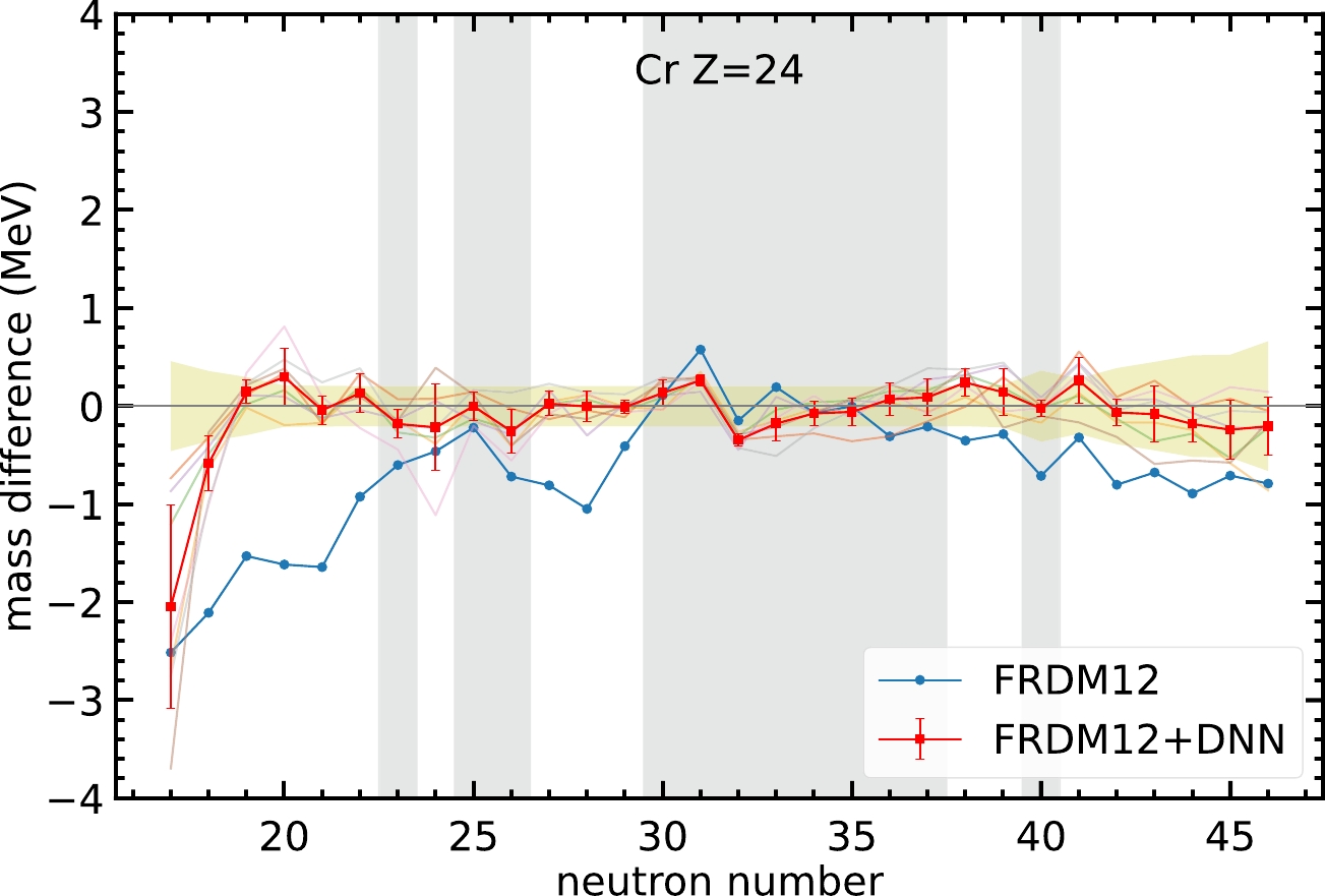

Figure 4.  (color online) Same as Fig. 3, but for Cr isotopes.

Finally, we must find whether there are any nuclei for which the mass prediction becomes worse after applying the neural network model. Out of the $ 3456 $ nuclei, there are $ 101 $ nuclei for which the DNN predictions are outside the yellow-hatched area and with a larger mass difference compared with the original FRDM12 model. Among these $ 101 $ nuclei, $ 92 $ have proton numbers less than $ 60 $, $ 63 $ occur in neutron-rich and proton-rich nuclei, and for the remaining cases, $ 16 $ might have a worse prediction because of odd-even staggering. For example, the Ba isotopes in Fig. 5 show good agreement in the mass prediction for the training set and large-neutron-number regions. However, for $ N=60 $ and $ 62 $, the neural network gives worse predictions compared to the FRDM12 model. This may occur because of two reasons. First, the nuclei $ N=60 $ and $ 62 $ are in the validation set and are not involved in the training of the model. Therefore, the overall performance of the nuclei in the validation set is not as good as that of the nuclei in the training set. Second, this neural network model still cannot tackle the odd-even staggering in light nuclei. Therefore, these two even-even nuclei do not exhibit better mass prediction after using the neural network, whereas the nearby even-odd nuclei in the training set exhibit better performance.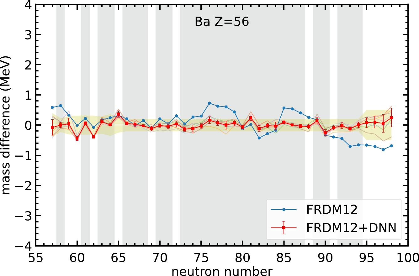

Figure 5.  (color online) Same as Fig. 3, but for Ba isotopes.

A DNN is applied to study the nuclear mass based on the FRDM12 model. Different hyperparameters, including activation functions, the learning rate, the number of hidden units, and initializers, are adjusted in a systematic way to achieve better model performance, as shown in Appendices A, B, C, and D. Finally, seven sets of hyperparameters with different regularizers and seed numbers have been selected. It is important that averaging the predictions given by several different sets of hyperparameters can provide not only the average values of mass predictions but also reliable estimations in the mass prediction uncertainties.

With the neural network, the RMS deviations between the experimental and theoretical masses are reduced from $ 0.603 $ to $ 0.200 $ MeV and $ 0.232 $ MeV for the training and validation sets, respectively. For most of the nuclei, this DNN model can give a better mass prediction compared with the FRDM12 model. Even for nuclei that have a poor mass prediction in the FRDM12 model, such as $ ^{41} $Cr and $ ^{42} $Cr, the DNN model can still reduce the RMS deviation and achieve a better mass prediction. However, there are still several nuclei with a worse mass prediction compared with the FRDM12 model, which may occur in the validation set with unsolved odd-even staggering problems. Further studies on these nuclei are required to improve the model, such as to provide a better description of the odd-even staggering in nuclei.

In the future, the same technique can be applied to other physics quantities related to nuclei. With the nuclear mass predicted in this study and by adjusting different hyperparameters, DNN models for different physics quantities, such as β-decay half-life and β-delayed neutron emission probability, can be generated and their performance can be compared with other current theoretical models to investigate whether this algorithm can improve the current predictions.

In this appendix, we explicitly investigate the impact of activation functions on the training performance.

The neural network model is able to approximate non-linear relations between inputs and outputs via the activation functions. Without using an activation function, the model is just a linear regression that cannot approximate non-linear relations. Figure A1 shows that without the activation function, the RMS deviation of the model will remain at approximately $ 0.6 $ MeV and no improvement can be made.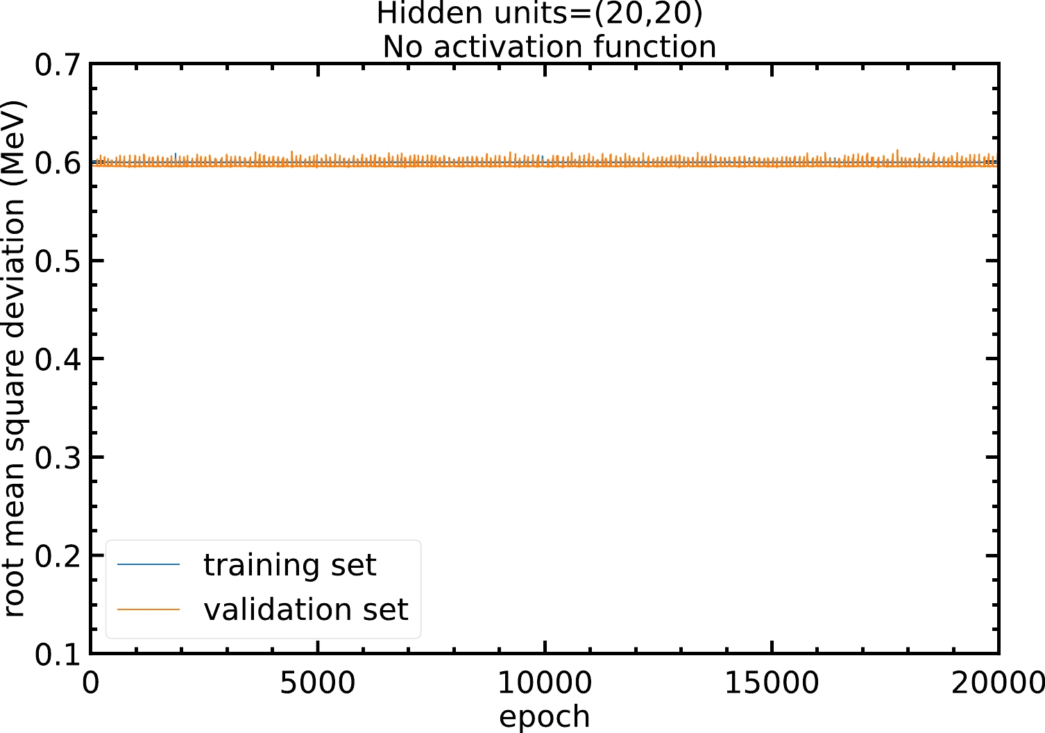

Figure A1.  (color online) RMS deviations of the training and validation sets in $ 20000 $ epochs with $ 20 $ hidden units in both hidden layers and no activation function. The blue and orange curves represent the RMS deviations of the training and validation sets, respectively.

Therefore, models with different activation functions are trained in this study. As shown in Fig. A2, with $ 20 $ hidden units, the RMS deviations of panels (a), (c), (h), and (i) are highly oscillating, and thus the corresponding activation functions are not recommended. In contrast, panels (b), (d), (e), (f), and (g) show a steady RMS deviation without large oscillations.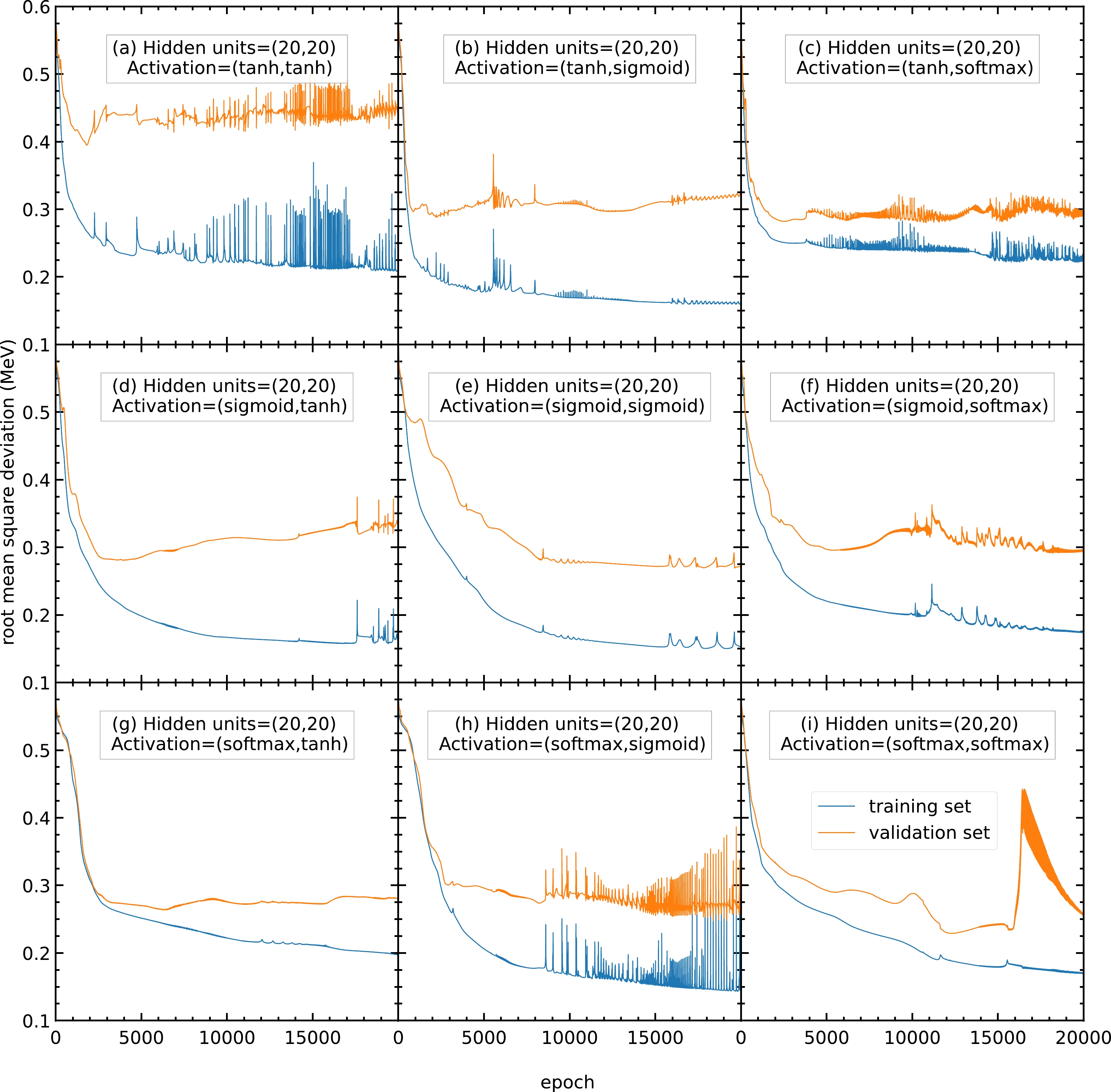

Figure A2.  (color online) RMS deviations of the training and validation sets in $ 20000 $ epochs with $ 20 $ hidden units in both hidden layers. The activation functions for the two hidden layers are selected as (a) (tanh, tanh), (b) (tanh, sigmoid), (c) (tanh, softmax), (d) (sigmoid, tanh), (e) (sigmoid, sigmoid), (f) (sigmoid, softmax), (g) (softmax, tanh), (h) (softmax, sigmoid), and (i) (softmax, softmax). The blue and orange curves represent the RMS deviations of the training and validation sets, respectively.

To find the best activation functions for the present mass models, the results from Fig. A3 with 22 hidden units are examined. Panel (b) is oscillating and not recommended. Panels (e) and (g) show RMS deviations larger than $ 0.3 $ MeV, which is larger than the RMS deviations of panels (d) and (f); therefore, panels (e) and (g) are not recommended. Panels (d) and (f) show small RMS deviations and less oscillation; hence, they are recommended for this mass model. In this study, the activation functions for the two hidden layers are chosen as (f) sigmoid and softmax functions for all the following calculations. If there are any future studies, the activation functions can be chosen as (d) sigmoid and tanh functions.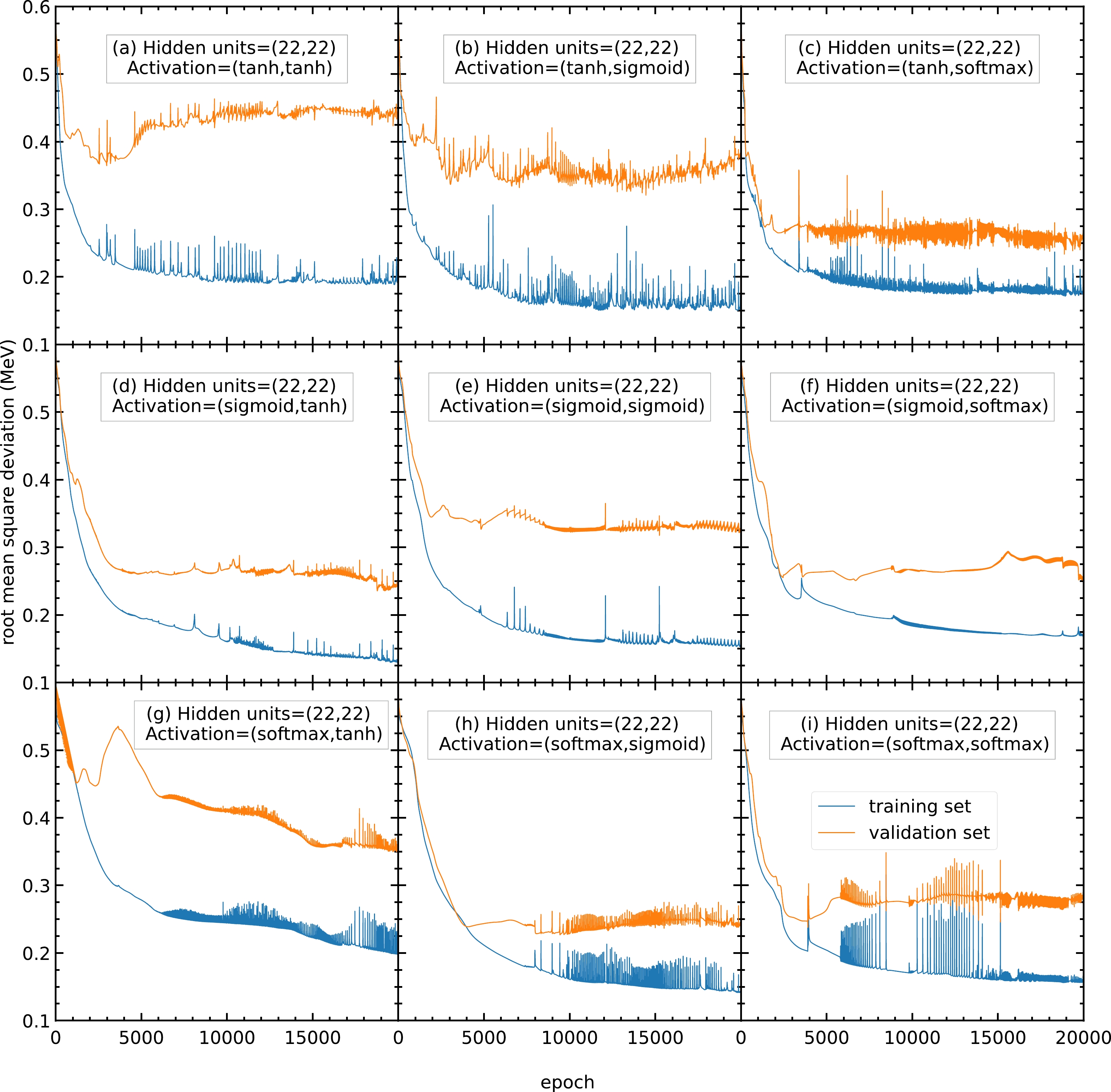

Figure A3.  (color online) Same as Fig. A2, but the number of hidden units in both hidden layers is $ 22 $.

In this appendix, we explicitly investigate the impact of the learning rate in the model algorithm on the training performance.

Fig. B1 shows the RMS deviations of the training and validation sets using the Adam algorithm with learning rates of $ 0.1 $, $ 0.01 $, $ 0.001 $, and $ 0.0001 $. As shown in Fig. B1(a), a model with a large learning rate causes the model parameters to oscillate and is unable to achieve the minimum; hence, its RMS deviations are highly oscillating with large values. A model with a smaller learning rate results in a larger number of epochs used to reach the lowest RMS deviation and is more time-consuming. Using a learning rate of $ 0.01 $, the RMS deviation for the validation set reaches approximately $ 0.27 $ MeV after $ 20000 $ epochs, as shown in Fig. B1(b). In contrast, using learning rates of $ 0.001 $ and $ 0.0001 $, the RMS deviations for the validation set are still approximately $ 0.43 $ and $ 0.54 $ MeV after $ 20000 $ epochs, as shown in Figs. B1(c) and B1(d), respectively. Therefore, the learning rate is selected as $ 0.01 $ for all the following calculations in this study.

Figure B1.  (color online) RMS deviations of the training and validation sets in $ 20000 $ epochs using the Adam algorithm as the optimizer with a learning rate of (a) $ 0.1 $, (b) $ 0.01 $, (c) $ 0.001 $, and (d) $ 0.0001 $. The blue and orange curves represent the RMS deviations of the training and validation sets, respectively.

In this appendix, we explicitly investigate the impact of the number of hidden units on the training performance.

Fig. C1 shows the RMS deviations of the training and validation sets with different numbers of hidden units per hidden layer, where the numbers of hidden units per hidden layer are varied from $ 10 $ to $ 70 $. Generally, a model with a small number of hidden units may result in an insufficient number of parameters for the model and be unable to achieve a small RMS deviation. It is confirmed by Fig. C1(a) that the RMS deviation for the validation set for $ 10 $ hidden units per hidden layer remains around $ 0.37 $ MeV after $ 10000 $ epochs.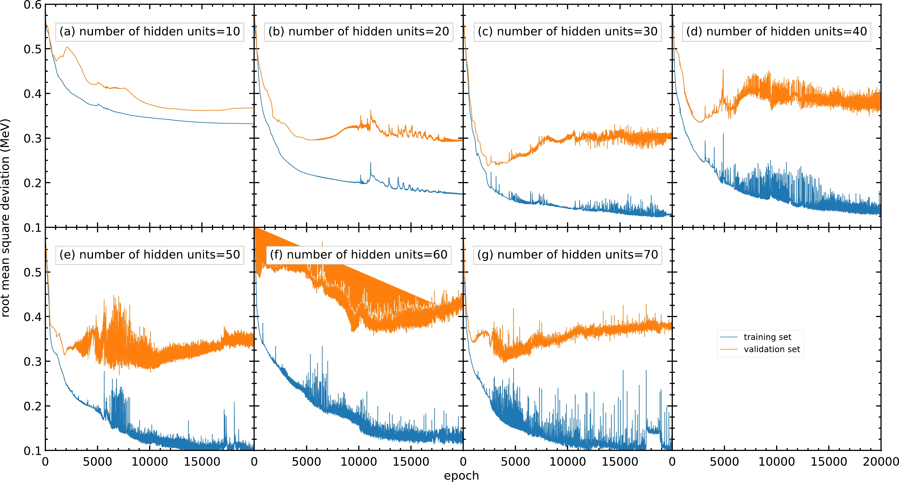

Figure C1.  (color online) RMS deviations of the training and validation sets in $ 20000 $ epochs with different numbers of hidden units per hidden layer within $ 10 $–$ 70 $: (a) $ 10 $, (b) $ 20 $, (c) $ 30 $, (d) $ 40 $, (e) $ 50 $, (f) $ 60 $, and (g) $ 70 $. The blue and orange curves represent the RMS deviations of the training and validation sets, respectively.

For a model with a larger number of hidden units, the number of parameters and the time used for training increase. Moreover, because the data in the training set generally include several types of noise, a large number of hidden units may lead to the overfitting problem and cause poor prediction outside the training set. As shown in panels (e), (f), and (g), although the RMS deviations for the training set are still decreasing after $ 10000 $ epochs, the RMS deviations for the validation set are increasing in this region, resulting in a poor mass prediction.

However, panel (b) shows less oscillation in the RMS deviation compared to panels (c) and (d). Meanwhile, $ 30 $ or more hidden units show no improvement in RMS deviation compared with $ 20 $ hidden units. For the above reasons, a number of hidden units of approximately $ 20 $ is selected.

To obtain a more precise number of hidden units, models with different numbers of hidden units from 16 to $ 24 $ are trained, and their performance is shown in Fig. C2. The performance of the models with different numbers of hidden units is similar, with approximately $ 0.25 $ MeV as the RMS deviation of the validation set. However, for models with 23 and 24 hidden units per hidden layer, the RMS deviations are oscillating; hence, these models are not recommended. For the remaining models with similar performance, the number of hidden units per hidden layer is chosen as 22 because this can provide more parameters without large oscillations or overfitting.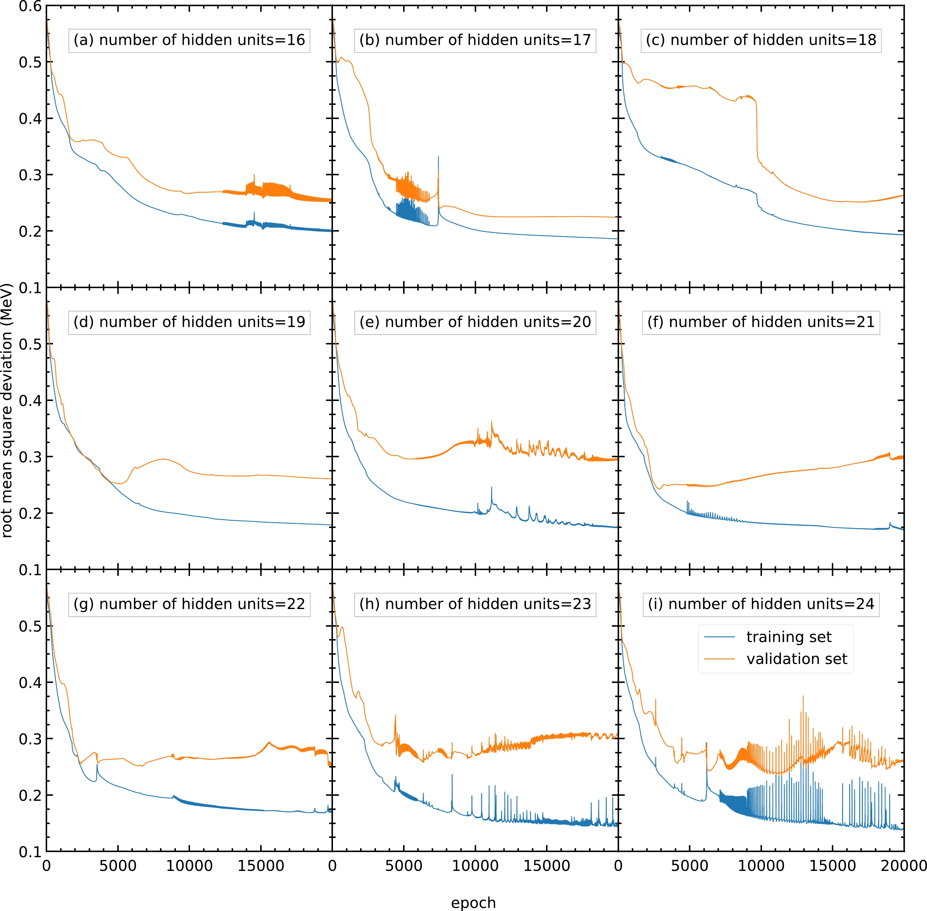

Figure C2.  (color online) RMS deviation of the training and validation sets in $ 20000 $ epochs with different numbers of hidden units per hidden layer within $ 16 $–$ 24 $: (a) $ 16 $, (b) $ 17 $, (c) $ 18 $, (d) $ 19 $, (e) $ 20 $, (f) $ 21 $, (g) $ 22 $, (h) $ 23 $, and (i) $ 24 $. The blue and orange curves represent the RMS deviations of the training and validation sets, respectively.

In this appendix, we explicitly investigate the impact of the initializers on the training performance.

The initial values of the parameters also affect the performance of the model. For example, when all the parameters are initialized with the same value, all the hidden units in the same hidden layer will be identical. Such a model is equivalent to a model with one hidden unit in each hidden layer. A model with a small number of hidden units has poor performance and cannot predict the output. As shown in Fig. C3(i), the RMS deviations remain at approximately $ 0.575 $ MeV during training.

Figure C3.  (color online) RMS deviations of the training and validation sets in $ 20000 $ epochs with different initializers for the parameters $ \{w^{(1)}_{ji},w^{(2)}_{kj}\} $ and bias $ \{w^{(1)}_{j0},w^{(2)}_{k0}\} $. The initializers adopted here include the standard normal, glorot normal, and zeros distributions [33]. The blue and orange curves represent the RMS deviations of the training and validation sets, respectively.

Therefore, we train the models with different sets of initial parameters ($ \{w^{(1)}_{ji}, w^{(2)}_{kj}\} $, $ \{w^{(1)}_{j0}, w^{(2)}_{k0}\} $). For the different sets of initial parameters trained, panels (a), (b), (c), (f), (g), and (h) exhibit RMS deviations of the validation set of around $ 0.23 $MeV. Among these six sets of initial parameters, panels (a), (b), and (f) give a steady RMS deviation curve during the entire training. Therefore, these three sets of initial parameters are recommended. In this study, initial parameters from panel (b) are selected for all the following calculations. Panels (a) and (f) can be used as the initial parameters for any future studies.