


 Abstract
 HTML
HTML Reference
 Related
 PDF
PDF


-
The deuteron, primarily comprising a bound state of a proton and neutron, is the simplest nontrivial nucleus in nature. It serves as an ideal system to study the structure of cold nuclear matter and nucleon-nucleon interactions. The deuteron has been a subject of experimental and theoretical scrutiny for over 80 years since its discovery and continues to be a vital area of research in nuclear and particle physics. Given the more comprehensive understanding of electromagnetic interactions, electron and photon scatterings from the deuteron, both with and without disintegration, have become principal methods for probing the deuteron structure [1−5]. The near-threshold production of
$ J/\psi $ from a deuteron target received great interest in recent years because of its sensitivity to the gluonic field and the nucleon-nucleon short-range correlations (SRCs). Furthermore, the final-state interaction in the incoherent scattering allows to investigate the$ J/\psi\,N $ scattering cross section at low energies [6−11]. As$ J/\psi $ in the final state is usually reconstructed from its decay channels to$ e^+e^- $ and$ \mu^+\mu^- $ , the lepton pair production is one of the dominant background reactions for the precise measurement of$ J/\psi $ production cross section, especially near the threshold.In addition to its role in studying nuclear structures, the deuteron is often used as a practical substitute for a neutron target, given the absence of stable, free neutron targets in researching nucleon structures. Electron deep inelastic scattering (DIS) from the deuteron is pivotal for the flavor separation in parton distribution functions. At the same time, it offers crucial insights into how nuclear matter modifies the partonic structure of a nucleon [12, 13]. Beyond parton distribution functions that describe the longitudinal momentum distribution of quarks and gluons in the nucleon, a primary objective of contemporary and future nuclear experiments is to precisely measure the three-dimensional partonic structures of the nucleon. Generalized parton distribution (GPD), encapsulating the transverse coordinate distribution of partons, represents a key physical quantity under investigation at Jefferson Lab and forthcoming electron-ion colliders [14−16]. A golden channel to access GPDs is the deeply virtual Compton scattering (DVCS), in which one can practically extract GPDs from the interference term between the DVCS amplitude and Bethe-Heitler (BH) amplitude [17−21]. Some light nuclei target DVCS experiments have been conducted at JLab [22,23]. Theoretical research related to these experiments focuses on extracting neutron GPDs and analyzing the nuclear effects on the GPDs of bound nucleons [24−28]. New processes with unique sensitivities to the x-dependence of GPDs are recently suggested [29, 30], and several other processes extended from the DVCS, such as the timelike Compton scattering (TCS) [31−37] and deeply virtual exclusive meson production (DVMP) [38−40], are also proposed as complementary channels to measure GPDs via the similar mechanism. These exclusive processes with deuteron target or beam supply an additional way to access neutron GPDs. Furthermore, due to the simpler nuclear structure of deuteron in comparison with other nuclei, it can serve as a promising beginning to study how the three dimensional image of nucleon is modified in the nuclear medium when the free nucleon GPDs are compared with those extracted from the process involved deuteron. In these types of measurements, the Bethe-Heitler process is a dominant background channel, which should be well understood.
The dilepton production in the deuteron breakup reaction through the BH mechanism shares the same final state particles as those in the TCS process, and the
$ J/\psi $ production with subsequent decay to a lepton pair from the deuteron. The BH contribution dominates the total cross section over the typical TCS region by more than one order of magnitude [31, 32]. Consequently, it acts as a major source of background noise, hindering the precise measurement of GPDs. For$ J/\psi $ production, the cross section is small and changes rapidly when the beam energy is near the threshold, and hence the yield from the BH channel is one of the key sources of systematic uncertainties in the analysis of$ J/\psi $ production. Furthermore, the final state interaction (FSI) also plays an important role in certain kinematic regions where the missing momentum of the undetected nucleon is not small [41−45], and thereby, it can shed light on the extraction of$ J/\psi\, N $ scattering cross section. All of the above necessitates a thorough investigation of BH lepton pair production from deuteron breakup reactions, with a particular emphasis on including the effects of FSIs.In this paper, we perform a complete calculation of the differential cross section of the dilepton production process in the deuteron breakup reaction via the BH mechanism. The lepton mass is kept finite not only to differentiate the results of
$ e^+e^- $ and$ \mu^+\mu^- $ production but also to physically regularize the collinear singularities. A relativistic covariant spectator theory [46−49] is utilized to describe the deuteron in terms of the proton and neutron, which has been proven successful in describing the elastic and inelastic electron deuteron scatterings [45, 50, 51] and the deuteron magnetic moment and electromagnetic form factors [52, 53]. The FSI is considered via the nucleon-nucleon scattering, which is parametrized in a Lorentz covariant form including all spin-dependent contributions following the formalism in [45]. However, other approaches, such as the Glauber approximation or the generalized eikonal approximation, are also commonly used in previous studies [41, 42, 44, 54−57]. With numerical results, we further analyze the impact of the FSI in comparison with the calculation using the plane wave impulse approximation (PWIA) and its kinematic dependence.The structure of this paper is outlined as follows. Sec. II introduces the theoretical framework for our calculations. This includes the kinematics of the process, covariant deuteron-nucleon vertex, and nucleon-nucleon rescattering in the final state. We derive the PWIA and FSI amplitudes, with comprehensive details provided in the appendix. In Sec. III, we present and discuss the numerical results for the differential cross section, focusing on the nearly singular behavior in certain kinematic regions and the impact of FSI, which is further dissected into on-shell and off-shell terms to elucidate their kinematic dependencies. The paper concludes with a summary and conclusions in Sec. IV.
-
We consider the process,
$ \begin{array}{*{20}{l}} \gamma(k) + d(P) \rightarrow p(p_1) + n(p_2) + l^-(p_3) + l^+(p_4), \end{array} $

(1) where the variables in parentheses denote the four momenta of the corresponding particles. Furthermore,
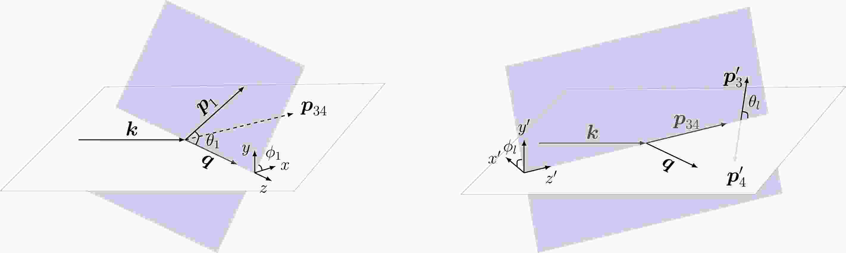
$ l^- $ and$ l^+ $ are a pair of charged leptons, such as$ e^-e^+ $ or$ \mu^- \mu^+ $ . The total four-momentum of the lepton pair in the final state is$ p_{34} = p_3 + p_4 $ , and the four-momentum transferred to the hadronic system is$ q = k - p_{34} = p_1 + p_2 - P $ . To describe the angular distribution of final state particles, it is convenient to specify a reference frame. Hence, we choose the deuteron rest frame, or sometimes referred to as the target rest frame, where$ \begin{array}{*{20}{l}} P &= (m_d, {{0{\boldsymbol{}}}}), \quad k = (E_\gamma, {{{\boldsymbol{k}}}}), \quad q = (\nu, {{{\boldsymbol{q}}}}). \end{array} $

(2) As illustrated in Fig. 1, we choose the photon momentum
$ {{{\boldsymbol{k}}}} $ and transferred momentum$ {{{\boldsymbol{q}}}} $ in the$ x-z $ plane. The direction of the proton momentum$ {{{\boldsymbol{p}}}}_1 $ is labeled by polar angle$ \theta_1 $ and azimuthal angle$ \phi_1 $ with respect to$ {{{\boldsymbol{q}}}} $ . The neutron momentum$ {{{\boldsymbol{p}}}}_2 $ , which is not shown in Fig. 1, is fixed by the momentum conservation$ {{{\boldsymbol{p}}}}_2 = {{{\boldsymbol{q}}}} - {{{\boldsymbol{p}}}}_1 $ , and we denote$ |{{{\boldsymbol{p}}}}_2| = p_m $ as the so-called missing momentum. The direction of the final-state lepton momentum$ {{{\boldsymbol{p}}}}_3 $ (or$ {{{\boldsymbol{p}}}}_4 $ ) can be easily defined in the center-of-mass frame of the lepton pair, where we label the polar angle and azimuthal angle of$ l^- $ as$ \theta_l $ and$ \phi_l $ , respectively, with respect to the direction of$ {{{\boldsymbol{p}}}}_{34} $ , which is nonzero in the target rest frame.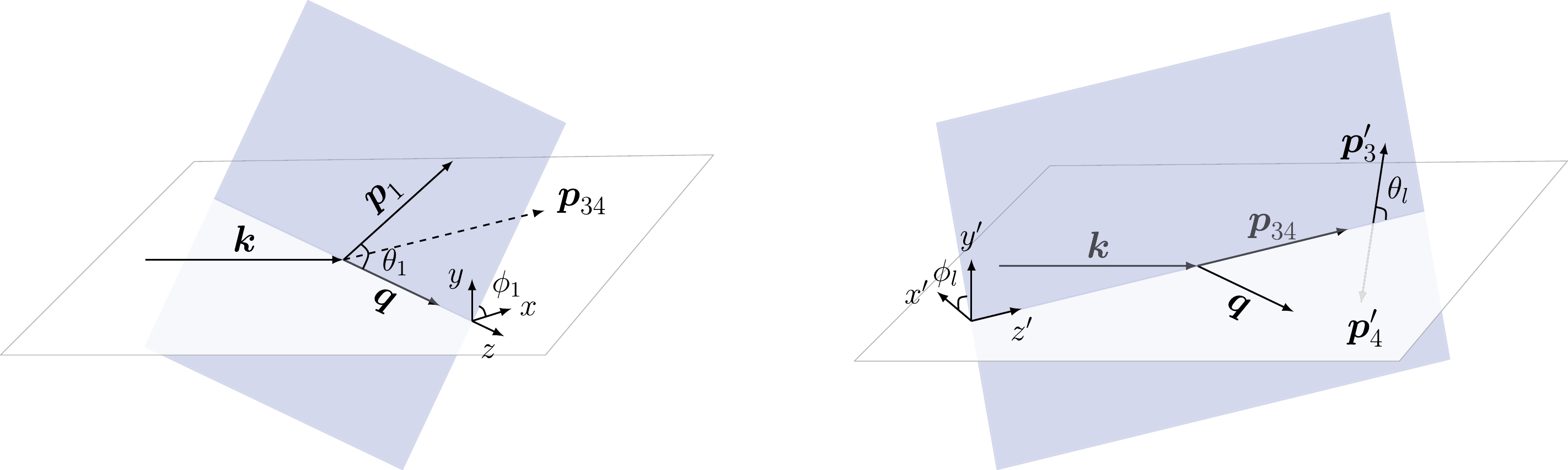
Figure 1. (color online) Kinematics for the dilepton photoproduction on the deuteron target. The lepton (anti-lepton) momentum in the center-of-mass frame of the lepton pair is labeled by
$p_3(p_4) $. With the kinematic variables defined above, we can express the differential cross section in the target rest frame as
$ \begin{aligned}[b] {{{\rm{d}}}} \sigma =& (2\pi)^4 \delta^{(4)}(k+P-p_1-p_2-p_3-p_4) \frac{1}{4E_\gamma m_d}\overline{\sum\limits_{\rm if}}|\mathcal{M}|^2 \\ & \times \frac{{{\rm{d}}^3} {\boldsymbol{p}}_1}{(2\pi)^3 2 E_1} \frac{{{\rm{d}}^3} {\boldsymbol{p}}_2}{(2\pi)^3 2 E_2} \frac{{{\rm{d}}^3} {\boldsymbol{p}}_3}{(2\pi)^3 2 E_3} \frac{{{\rm{d}}^3} {\boldsymbol{p}}_4}{(2\pi)^3 2 E_4}\; , \end{aligned} $

(3) where
$ E_i=\sqrt{m_i^2+{\boldsymbol{p}}_i^2} $ denotes the energy of corresponding particles,$ m_1 = m_2 =m $ denotes the nucleon mass, and$ m_3 = m_4 = m_l $ is the lepton mass. Symbol$ {\overline{\sum}_{\rm if}} $ represents the average over spin states in the initial state and the sum over spin states in the final state.In this study, we consider the lepton pair production via the Bethe-Heitler mechanism. With one-photon-exchange approximation, we can express the invariant amplitude square as
$ \overline{\sum\limits_{\rm if}}|\mathcal{M}|^2 = \frac{e^6}{t^2}L^{\mu\nu}W_{\mu\nu}\; , $

(4) where
$ t=q^2 $ denotes the transferred momentum square. The unpolarized leptonic tensor$ L^{\mu\nu} $ is as follows:$ \begin{aligned}[b] L^{\mu \nu}=&-\frac{1}{2} \operatorname{Tr}\left\{\left(\not p_{3}+m_l\right) \Bigg[\gamma^{\alpha} \frac{\not {p}_{3}-\not {k}+m_l}{\left(p_{3}-k\right)^{2}-m_l^{2}} \gamma^{\mu}\right.\\&+\gamma^{\mu} \frac{\not {k}-\not {p}_{4}+m_l}{\left(k-p_{4}\right)^{2}-m_l^{2}} \gamma^{\alpha}\Bigg] \\ & \times \left(\not {p}_{4}-m_l\right) \Bigg[\gamma^{\nu} \frac{\not {p}_{3}-\not {k}+m_l}{\left(p_{3}-k\right)^{2}-m_l^{2}} \gamma_{\alpha}\\&\left. + \gamma_{\alpha} \frac{\not {k}-\not {p}_{4}+m_l}{\left(k-p_{4}\right)^{2}-m_l^{2}} \gamma^{\nu}\Bigg]\right\}\; , \end{aligned} $

(5) which is the same as the one for the Bethe-Heitler process [58]. The information on nuclear structure is contained in the hadronic tensor,
$ W_{\mu\nu}=(2m)^2\overline{\sum\limits_{{\rm{if}}}}J_\mu(q) J_\nu^{\dagger}(q)\; , $

(6) where
$ J_\mu(q)=\langle{\boldsymbol{p}}_{1} s_{1}; {\boldsymbol{p}}_{2} s_{2}\left|\hat{J}_{\mu}(0)\right| {\boldsymbol{P}} \lambda_{d}\rangle $ is the nuclear electromagnetic current matrix element in the momentum space, and$ \lambda_d $ ,$ s_1 $ , and$ s_2 $ denote the spin states of the initial deuteron, final proton, and final neutron, respectively. A factor of$ \sqrt{2m} $ is inserted for each nucleon spinor to be consistent with the normalization convention in following calculations, where the nucleon spinors are normalized as$ u^{\dagger}({{{\boldsymbol{p}}}},s) u({{{\boldsymbol{p}}}},s') = E_{\boldsymbol{p}}/m $ . The current conservation requires the following:$ \begin{array}{*{20}{l}} q^\mu J_\mu(q) = \nu J^0(q) - {\boldsymbol{q}} \cdot {\boldsymbol{J}}(q)=0\; . \end{array} $

(7) However, it is not an exact identity in the model calculation. We consider
$ {\boldsymbol{q}} $ along the z-direction and replace explicit$ J_z(q) $ dependence by$ \left(\nu/|{\boldsymbol{q}}|\right) J^0(q) $ in the numerical calculation to restore the current conservation law explicitly [59−62].After integrating the four-momentum conservation δ-function and a global azimuthal angle of final-state particles with respect to the photon axis, we obtain a seven-fold differential cross section. For convenience, we adopt the invariant mass square of the proton and neutron
$ s_{pn}=(p_1+p_2)^2 $ and the invariant mass square of the lepton pair$ s_{ll}=(p_3+p_4)^2 $ as variables. Then, the differential cross section can be expressed as$ \begin{aligned}[b] {{{\rm{d}}}} \sigma =&\frac{\alpha^3}{8(4\pi)^4}\frac{|{\boldsymbol{p}}_1|^2\beta}{m_d^2 E_\gamma^2 t^2}\frac{L^{\mu\nu}W_{\mu\nu}}{||{\boldsymbol{p}}_1|(m_d+\nu)-E_1|{\boldsymbol{q}}|\cos \theta_1|}\\&\times{{\rm{d}}} \Omega_p {{\rm{d}}} \Omega_{ll}{{\rm{d}}}s_{ll}{{\rm{d}}}s_{pn}{{\rm{d}}}t\; , \end{aligned}$

(8) where
$ \Omega_p $ denotes the solid angle of the proton with$ {{{\rm{d}}}}\Omega_p = {{{\rm{d}}}}\cos\theta_1 {{{\rm{d}}}}\phi_1 $ ,$ \Omega_{ll} $ denotes the solid angle of$ l^- $ in the lepton pair center-of-mass frame with$ {{{\rm{d}}}}\Omega_{ll} = {{{\rm{d}}}}\cos\theta_l {{{\rm{d}}}}\phi_l $ , and β denotes the lepton velocity given by$ \beta=\sqrt{1-\frac{4m_l^2}{s_{ll}}}\; , $

(9) and
$ \alpha = e^2/(4\pi) $ corresponds to the electromagnetic fine structure constant. The derivation from Eq. (3) to Eq. (8) is provided in Appendix A. -
Firstly, we consider the impulse approximation (IA), in which the reaction is viewed as the Bethe-Heitler process from a quasi-free nucleon in the deuteron. The mechanism of this plane wave (PW) contribution is depicted by the Feynman amplitudes in Fig. 2. In this case, electromagnetic current matrix element can be expressed as
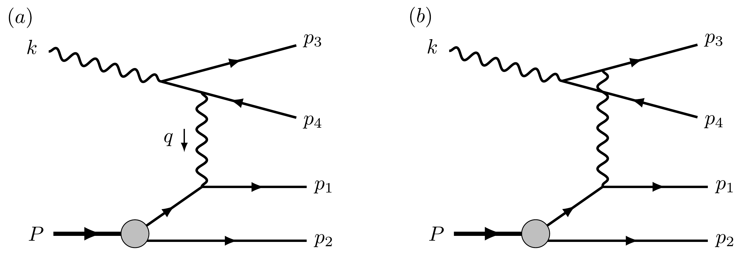
Figure 2. Feynman diagrams for the PWIA in the one-photon-exchange approximation.
$ \begin{aligned}[b] J_{{\rm{PW}}}^\mu(q) =& \langle{\boldsymbol{p}}_{1} s_{1} ; {\boldsymbol{p}}_{2} s_{2}\left|\hat{J}^{\mu}\right| {\boldsymbol{P}} \lambda_{d}\rangle_{{\rm{PW}}}\\ =&\bar{u}\left({\boldsymbol{p}}_{1}, s_{1}\right) \Gamma_N^{\mu}(q) G_{0}\left(P-p_{2}\right) \\&\times\Gamma_{\lambda_{d}}\left(p_{2}, P\right)C \bar{u}^{T}\left({\boldsymbol{p}}_{2}, s_{2}\right)\; , \end{aligned} $

(10) where
$C=-{\rm i}\gamma^0\gamma^2$ denotes the charge conjugation operator, and$ G_0 $ denotes the bare nucleon propagator expressed as follows:$ G_0(p)=\frac{\not {p}+m}{m^2-p^2-{\rm i}\epsilon}\; , $

(11) where
$ \epsilon $ denotes a positive infinitesimal number. The nucleon electromagnetic current vertex$ \Gamma_N^\mu (q) $ is parametrized as$ \Gamma_N^\mu(q)=F_1(Q^2)\gamma^\mu+\frac{F_2(Q^2)}{2m}{\rm i}\sigma^{\mu\nu} q_\nu\; , $

(12) where
$ Q^2 = -t $ and$ F_1(Q^2) $ and$ F_2(Q^2) $ denote nucleon's Dirac and Pauli form factors. In numerical calculations, we use the fit of nucleon electromagnetic form factors in Ref. [63]. The deuteron-proton-neutron vertex can be expressed as$ \begin{array}{*{20}{l}} \Gamma_{\lambda_d}(p_2,P) = \Gamma_D^\mu(p_2,P)\; \xi^{\lambda_d}_{\mu}(P), \end{array} $

(13) where
$ \xi_\mu^{\lambda_d}(P) $ denotes the deuteron polarization vector and$ \Gamma_D^\mu(p_2,P) $ denotes the covariant vertex function with P and$ p_2 $ on-shell. According to the Lorentz structure, the vertex function can be expressed as [46, 48, 49]:$ \Gamma_{D}^\mu(k_2,P)\equiv F \gamma^\mu+\frac{G}{m} k^\mu-\frac{m-\not {k}_1}{m}\left(H \gamma^\mu+\frac{I}{m} k^\mu\right)\; , $

(14) where
$ k = (k_2 - k_1)/2 $ denotes the relative four-momentum of the two nucleons and$ k_1 = P - k_2 $ denotes the momentum of the off-shell nucleon. The scalar functions F, G, H, and I encode the nucleonic structure of the deuteron and can be evaluated from the deuteron wave functions. Explicit expressions of these functions are provided in Appendix B and more details can be found in Refs. [47, 52].Substituting Eq. (10) into Eq. (6), we obtain the hadronic tensor in the plane wave impulse approximation (PWIA) as
$ \begin{aligned}[b] W^{\mu\nu}_{\rm PW}=& (2m)^2\overline{\sum\limits_{{\rm{if}}}}J_{{\rm{PW}}}^\mu(q) J^{\nu\,\dagger}_{{\rm{PW}}}(q) \\ &={{\rm{Tr}}}\Bigg[\Gamma_N^{\mu}(q) \frac{\not {P}-\not {p}_2+m}{m^2-(P-p_2)^2} \Gamma_D^\alpha\left(p_{2}, P\right)\left(\not {p}_2-m\right)\\&\times\widetilde{\Gamma}_D^\beta\frac{\not {P}-\not {p}_2+m}{m^2-(P-p_2)^2}\widetilde{\Gamma}_N^\nu \left(\not {p}_1+m\right)\Bigg]\\ &\times \frac{1}{3}\sum\limits_{\lambda_d=1}^3 \xi_\alpha^{\lambda_d}(P)\; \xi^{*\,\lambda_d}_\beta(P)\; , \end{aligned} $

(15) where
$ \widetilde{\Gamma}_N^\nu =\gamma^0 \Gamma_N^{\nu\,\dagger} \gamma^0=F_1(Q^2)\gamma^\nu-\frac{F_2(Q^2)}{2m}{\rm i}\sigma^{\nu\eta} q_\eta\; , $

(16) $ \widetilde{\Gamma}^\beta_{D}=\gamma^0 \Gamma^{\beta\,\dagger}_{D} \gamma^0=F \gamma^\beta+\frac{G}{m} p^\beta-\left(H \gamma^\beta+\frac{I}{m} p^\beta\right)\frac{m-\not {p}_1}{m}\; , $

(17) and
$ p=\dfrac{1}{2}(p_2-p_1+q) $ . The derivation of Eq. (15) is provided in Appendix C. -
In the PWIA, the spectator nucleon remains uninvolved in the reaction. Although this approximation is commonly employed in numerous Monte Carlo simulations, its accuracy requires quantitative assessment for precise measurements. Our approach accounts for scenarios where one nucleon, after being struck by the virtual photon, interacts with the other nucleon prior to exiting. This FSI mechanism is depicted in Fig. 3. In this case, the proton leg and neutron leg of the deuteron-proton-neutron vertex can be both off-shell, and this type of vertex function is explored in Ref. [52], in which the amplitude requires a four-dimensional integration over the internal momentum k. In this study, we simplify the calculation by applying the covariant spectator theory [46−49], in which the nucleon that is not directly struck by the virtual photon is set on-shell, and the four-dimensional integration is replaced by
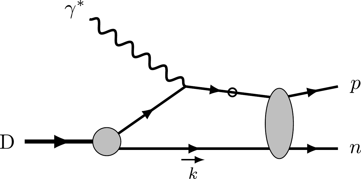
Figure 3. Contribution of final state interactions to the electromagnetic current matrix element. The fermion line with "
$ \circ $ " represents the particle that can be off-shell, and the propagator will be decomposed into positive energy contribution and negative energy contribution.$ \int \frac{ {{{\rm{d}}}}^3 {\boldsymbol{k}}}{(2\pi)^3}\frac{m}{E_{{\boldsymbol{k}}}}\; . $

(18) This method has been utilized in the study of the elastic electron-deuteron scattering [50] and electrodisintegration of the deuteron [45], and the results are in good agreement with experimental data.
To evaluate the FSI effect, we should calculate the rescattering between the knocked-out nucleon and recoil nucleon. According to the Dirac matrix structure, the nucleon-nucleon (NN) scattering matrix can be parametrized as [45, 64, 65]
$ \begin{aligned}[b] M=&F_S(s_N,t_N) {\boldsymbol{1}}_1 {\boldsymbol{1}}_2 + F_V(s_N,t_N) (\gamma^\mu)_1 (\gamma_\mu)_2 \\&+ F_T(s_N,t_N) (\sigma^{\mu\nu})_1(\sigma_{\mu\nu})_2\\ &+ F_P(s_N,t_N) (\gamma^5)_1 (\gamma^5)_2 \\&+ F_A(s_N,t_N) (\gamma^5 \gamma^\mu)_1 (\gamma^5 \gamma_\mu)_2\; , \end{aligned} $

(19) where subscripts "
$ 1 $ " and "$ 2 $ " of the γ-matrices indicate the spinor space of the corresponding nucleon.$ F_S $ ,$ F_V $ ,$ F_T $ ,$ F_P $ , and$ F_A $ denote scalar functions of$ s_N $ and$ t_N $ , which are the Mandelstam variables for the NN elastic scattering. Considering the spin states of the nucleons, the NN scattering matrix can be alternatively expanded as [64, 66]$ \begin{aligned}[b] M\left({\boldsymbol{k}}_{f}, {\boldsymbol{k}}_{i}\right)=&\frac{1}{2}[(a+b)+(a-b)\left({\boldsymbol{\sigma}}_{1}, {\boldsymbol{n}}\right)\left({\boldsymbol{\sigma}}_{2}, {\boldsymbol{n}}\right)\\&+(c+d)\left({\boldsymbol{\sigma}}_{1}, {\boldsymbol{m}}\right)\left({\boldsymbol{\sigma}}_{2}, {\boldsymbol{m}}\right)\\ &+(c-d)\left({\boldsymbol{\sigma}}_{1}, {\boldsymbol{l}}\right)\left({\boldsymbol{\sigma}}_{2}, {\boldsymbol{l}}\right)+e\left({\boldsymbol{\sigma}}_{1}+{\boldsymbol{\sigma}}_{2}, {\boldsymbol{n}}\right)]\; , \end{aligned} $

(20) where
$ {{{\boldsymbol{k}}}}_i $ and$ {{{\boldsymbol{k}}}}_f $ denote momenta of the nucleon before and after the scattering in the NN center-of-mass frame, in which the basis vectors can be constructed as follows:$ {\boldsymbol{l}}=\frac{{\boldsymbol{k}}_{f}+{\boldsymbol{k}}_{i}}{\left|{\boldsymbol{k}}_{f}+{\boldsymbol{k}}_{i}\right|}, \quad {\boldsymbol{m}}=\frac{{\boldsymbol{k}}_{f}-{\boldsymbol{k}}_{i}}{\left|{\boldsymbol{k}}_{f}-{\boldsymbol{k}}_{i}\right|}, \quad {\boldsymbol{n}}=\frac{{\boldsymbol{k}}_{i} \times {\boldsymbol{k}}_{f}}{\left|{\boldsymbol{k}}_{i} \times {\boldsymbol{k}}_{f}\right|}\; . $

(21) Furthermore,
$ ({\boldsymbol{\sigma}}_j,{\boldsymbol{v}}) $ represents the projection of the spin Pauli matrix$ {\boldsymbol{\sigma}} $ of the jth particle on direction$ {\boldsymbol{v}}={{{\boldsymbol{l}}}} $ ,$ {{{\boldsymbol{m}}}} $ , and$ {{{\boldsymbol{n}}}} $ . Amplitudes a, b, c, d, and e are complex functions of momentum$ |{\boldsymbol{k}}_i|=|{{{\boldsymbol{k}}}}_f| = \sqrt{s_N-4m^2}/2 $ and scattering angle θ, which can be expressed in terms of Mandelstem variables as$ \cos \theta=1 + \frac{2 t_N}{s_N-4m^2}\; . $

(22) These two parametrizations of the NN scattering matrix can be related through the helicity amplitudes as demonstrated in Appendix D. The partial wave expansion for amplitudes a, b, c, d, and e is presented in Ref. [67]. In numerical calculations, we use the phase shift analysis in Refs. [68, 69], and the phase shift data are available from the SAID program [70].
Although the recoil nucleon is set on-shell in the covariant spectator theory, the struck nucleon can be off-shell before the rescattering. In principle, additional terms in the NN scattering matrix can be included with one of the nucleon off-shell [71]. In this study, we follow the approach in Ref. [45] by introducing a form factor
$ F_N(p^2) $ to account for the off-shell effect and keep the NN scattering matrix parametrization in the same form as Eq. (19). Furthermore, scalar functions$ F_j(s_N,t_N) $ with$ j=S $ , V, T, P, and A are then replaced by$ \begin{array}{*{20}{l}} F_j(s_N,t_N) \rightarrow F_j(s_N,t_N,u_N) F_N(s_N+t_N+u_N-3m^2)\; , \end{array} $

(23) where
$ \begin{array}{*{20}{l}} F_N(p^2)=\dfrac{(\Lambda_N^2-m^2)^2}{(p^2-m^2)^2+(\Lambda_N^2-m^2)^2}\; , \end{array} $

(24) and p represents the four-momentum of the off-shell nucleon. If one of the incident nucleons is off-shell, the amplitude of three momentum of nucleons before scattering is
$ |{\boldsymbol{k}}_i|=\frac{\sqrt{(4m^2-t_N-u_N)^2-4m^2 s_N}}{2\sqrt{s_N}}\; . $

(25) In the final states, both nucleons are on-shell. Hence,
$ |{{{\boldsymbol{k}}}}_f| $ is still$ \sqrt{s_N-4m^2}/2 $ . Then, the scattering angle θ is expressed as$\cos \theta=\frac{t_N-u_N}{4|{\boldsymbol{k}}_i||{\boldsymbol{k}}_f|}= \frac{t_N-u_N}{\sqrt{1 - 4m^2/s_N}\sqrt{(4m^2 - t_N - u_N)^2-4m^2 s_N}}\; . $

(26) When
$ p^2=m^2 $ , the form factor$ F_N(m^2)=1 $ , and the scattering angle θ reduces back to the regular expression for the on-shell NN scattering. Furthermore,$ \Lambda_N $ denotes a phenomenological parameter, which we select to be$1.2~{\rm{GeV}}$ as suggested in Ref. [45].With Eqs. (18) and (19), the FSI contribution to the current matrix element can be expressed as
$ \begin{aligned}[b] J_{{\rm{FSI}}}^\mu(q)_{{\rm{if}}}=&\langle{\boldsymbol{p}}_{1} s_{1}; {\boldsymbol{p}}_{2} s_{2}\left|\hat{J}^{\mu}\right| {\boldsymbol{P}} \lambda_{d}\rangle_{{\rm{FSI}}} =\int \frac{{\rm d}^{3} {\boldsymbol{k}}}{(2 \pi)^{3}} \frac{m}{E_{k}} \bar{u}_{\alpha}\left({\boldsymbol{p}}_{1}, s_{1}\right) \bar{u}_{\beta}\left({\boldsymbol{p}}_{2}, s_{2}\right) M_{\alpha \alpha^\prime ; \beta \beta^\prime}\left(p_{1}, p_{2} ; k\right) \\ & \times G_{0\, \alpha^\prime \eta}\left(P+q-k\right) \Gamma_{N\,\eta \eta^\prime}^{\mu}(q) G_{0\, \eta^\prime \zeta} \left(P-k\right)( \Gamma_{\lambda_{d }}C)_{\zeta \zeta^\prime}\left(k, P\right)\Lambda_{\beta^\prime \zeta^\prime}^+\left({\boldsymbol{k}}\right)\; . \end{aligned} $ 
(27) Then, we decompose the bare nucleon propagator into the positive and the negative energy terms,
$ \begin{aligned}[b] G_{0}(p) =&-\frac{m}{E_{p}} \sum\limits_{s}\left[\frac{u(\boldsymbol{p}, s) \bar{u}(\boldsymbol{p}, s)}{p^{0}-E_{p}+{\rm i} \epsilon}+\frac{v(-\boldsymbol{p}, s) \bar{v}(-\boldsymbol{p}, s)}{p^{0}+E_{p}-{\rm i} \epsilon}\right] \\ =&-\frac{m}{E_{p}}\left[\frac{\Lambda_+(\boldsymbol{p})}{p^{0}-E_{p}+{\rm i} \epsilon}-\frac{\Lambda_-(-\boldsymbol{p})}{p^{0}+E_{p}-{\rm i} \epsilon}\right], \end{aligned} $

(28) where projection operators
$ \Lambda_{\pm} $ are defined as$ \Lambda_+({\boldsymbol{p}})=\frac{\not {\bar{p}}+m}{2m} = \sum\limits_s u({\boldsymbol{p}},s)\bar{u}({\boldsymbol{p}},s)\; , $

(29) $ \Lambda_-({\boldsymbol{p}})=-\frac{\not {\bar{p}}-m}{2m} = -\sum\limits_s v({\boldsymbol{p}},s)\bar{v}({\boldsymbol{p}},s)\; , $

(30) which correspond to the positive and the negative energy solutions, respectively, and
$ \bar{p} $ denotes the on-shell four-momentum. Furthermore, we use the relation$ \frac{1}{p^{0}-E_{p}+{\rm i} \epsilon}=-{\rm i} \pi \delta\left(p^{0}-E_{p}\right)+\frac{\mathcal{P.V.}}{p^{0}-E_{p}} $

(31) to express the positive energy term into two parts. Hence, Eq. (27) is decomposed into three parts,
$ \begin{array}{*{20}{l}} J_{{\rm{FSI}}}^\mu(q)_{{\rm{if}}}=J_{{\rm{FSI}}}^\mu(q)^{{\rm{A}}}_{{\rm{if}}}+J_{{\rm{FSI}}}^\mu(q)^{{\rm{B}}}_{{\rm{if}}}+J_{{\rm{FSI}}}^\mu(q)^{{\rm{C}}}_{{\rm{if}}}\; , \end{array} $

(32) where
$ \begin{aligned}[b]\\[-8pt] J_{{\rm{FSI}}}^\mu(q)^{{\rm{A}}}_{{\rm{if}}} =& \sum\limits_{s}\int \frac{{\rm d}^{3} {\boldsymbol{k}}}{(2 \pi)^{3}} ({\rm i}\pi)\frac{m}{E_{k}}\frac{m}{E_{P+q-k}}\delta(P^0+q^0-E_k-E_{P+q-k})\\ & \times \bar{u}_{\alpha}\left({\boldsymbol{p}}_{1}, s_{1}\right) \bar{u}_{\beta}\left({\boldsymbol{p}}_{2}, s_{2}\right) M_{\alpha \alpha^\prime ; \beta \beta^\prime}\left(p_{1}, p_{2} ; k\right) u_{\beta^\prime}\left({\boldsymbol{k}}, s\right)\\ & \times \Lambda^+_{ \alpha^\prime \eta}\left({\boldsymbol{P}}+{\boldsymbol{q}}-{\boldsymbol{k}}\right) \Gamma_{N\,\eta \eta^\prime}^{\mu}(q) G_{0\, \eta^\prime \zeta} \left(P-k\right)( \Gamma_{\lambda_{d }}C)_{\zeta \zeta^\prime}\left(k, P\right)\bar{u}^T_{\zeta^\prime}\left({\boldsymbol{k}}, s\right)\; \end{aligned} $ 
(33) is the on-shell positive energy contribution,
$ \begin{aligned}[b] J_{{\rm{FSI}}}^\mu(q)^{{\rm{B}}}_{{\rm{if}}} =& \sum\limits_{s}\int \frac{{\rm d}^{3} {\boldsymbol{k}}}{(2 \pi)^{3}} (-1)\frac{m}{E_{k}}\frac{m}{E_{P+q-k}}\frac{\mathcal{P.V.}}{P^0+q^0-E_k-E_{P+q-k}}\\ & \times \bar{u}_{\alpha}\left({\boldsymbol{p}}_{1}, s_{1}\right) \bar{u}_{\beta}\left({\boldsymbol{p}}_{2}, s_{2}\right) M_{\alpha \alpha^\prime ; \beta \beta^\prime}\left(p_{1}, p_{2} ; k\right) u_{\beta^\prime}\left({\boldsymbol{k}}, s\right)\\ & \times \Lambda^+_{ \alpha^\prime \eta}\left({\boldsymbol{P}}+{\boldsymbol{q}}-{\boldsymbol{k}}\right) \Gamma_{N\,\eta \eta^\prime}^{\mu}(q) G_{0\, \eta^\prime \zeta} \left(P-k\right)( \Gamma_{\lambda_{d }}C)_{\zeta \zeta^\prime}\left(k, P\right)\bar{u}^T_{\zeta^\prime}\left({\boldsymbol{k}}, s\right)\; \end{aligned} $

(34) is the principal value integral (off-shell) positive energy contribution, and
$ \begin{aligned}[b] J_{{\rm{FSI}}}^\mu(q)^{{\rm{C}}}_{{\rm{if}}}=& \sum\limits_{s}\int \frac{{\rm d}^{3} {\boldsymbol{k}}}{(2 \pi)^{3}} \frac{m}{E_{k}}\frac{m}{E_{P+q-k}}\frac{1}{P^0+q^0-E_k+E_{P+q-k}-{\rm i}\epsilon}\\ & \times \bar{u}_{\alpha}\left({\boldsymbol{p}}_{1}, s_{1}\right) \bar{u}_{\beta}\left({\boldsymbol{p}}_{2}, s_{2}\right) M_{\alpha \alpha^\prime ; \beta \beta^\prime}\left(p_{1}, p_{2} ; k\right) u_{\beta^\prime}\left({\boldsymbol{k}}, s\right)\\ & \times \Lambda^-_{ \alpha^\prime \eta}\left({\boldsymbol{k}}-{\boldsymbol{P}}-{\boldsymbol{q}}\right) \Gamma_{N\,\eta \eta^\prime}^{\mu}(q) G_{0\, \eta^\prime \zeta} \left(P-k\right)( \Gamma_{\lambda_{d }}C)_{\zeta \zeta^\prime}\left(k, P\right)\bar{u}^T_{\zeta^\prime}\left({\boldsymbol{k}}, s\right)\; \end{aligned} $

(35) is the negative energy contribution. Furthermore,
$ J_{{\rm{FSI}}}^\mu(q)^{{\rm{A}}}_{{\rm{if}}} + J_{{\rm{FSI}}}^\mu(q)^{{\rm{B}}}_{{\rm{if}}} $ is shown in Fig. 4(a), and$ J_{{\rm{FSI}}}^\mu(q)^{{\rm{C}}}_{{\rm{if}}} $ is shown in Fig. 4(b). Given that the negative energy part (anti-nucleon propagation) is much smaller than the positive energy part (nucleon propagation), we ignore the contribution from Eq. (35) in the calculation. This is the same approximation as adopted in Ref. [45].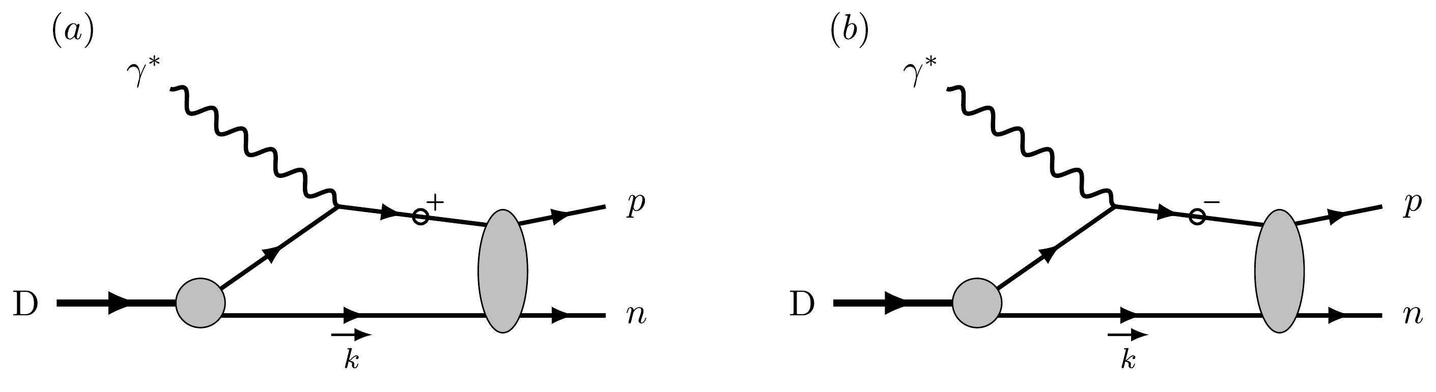
Figure 4. Decomposition of the FSI amplitude. The fermion line with "
$ \circ ^{+} $ " represents the positive energy contribution, including the on-shell term and off-shell principal value term, and the fermion line with "$ \circ ^{-} $ " represents the negative energy contribution. -
In this section, we present the numerical results for the unpolarized differential cross section. We first discuss the angular distribution of the differential cross section in the PWIA and singular feature of the cross section at some kinematics for the
$ e^+e^- $ production. Then, we discuss the FSI effect on the differential cross section and impact from the on-shell and off-shell contributions, respectively. Furthermore, we consider the effect arising from possible interference between the proton and neutron amplitudes. -
Given the lepton pair production via the BH process is a dominant background channel for the measurement of
$ J/\psi $ production near the threshold, we choose the photon energy at$ 8.5~\rm GeV $ , which is just above the$ J/\psi $ production threshold from free nucleons and is accessible at Jefferson Lab. With four particles in the final state, the complete differential cross section is seven-fold after eliminating an azimuthal symmetric angle for the scattering from unpolarized deuteron target.In Fig. 5, we plot the differential cross section as a function of the lepton azimuthal angle
$ \phi_l $ at several values of$ \theta_l = 10^\circ $ ,$ 90^\circ $ , and$ 170^\circ $ to show the polar angle dependence. Furthermore,$ s_{ll} = 9.6~\rm GeV^2 $ is set as the mass square of$ J/\psi $ ,$ s_{pn} = 5~\rm GeV^2 $ , and$ t = -1.5~\rm GeV^2 $ are chosen at some typical values, and$ p_1 = 1.4~\rm GeV $ and$ \phi_1 = 180^\circ $ are fixed for the struck proton. As observed from Fig. 5, the cross section is large when$ \theta_l $ is close to$ 0^\circ $ or$ 180^\circ $ . At this limit, the emitted lepton or antilepton is collinear to$ {{{\boldsymbol{p}}}}_{34} $ , the lepton pair momentum. Although the cross section does not exhibit singularities in this kinematics region, the polar angle of$ {{{\boldsymbol{p}}}}_{34} $ is small for the particular kinematic choice here. Hence, the enhancement around$ \phi_l = 180^\circ $ or$ 0^\circ $ is actually from the singularity when one of the lepton pair is collinear with the incident photon as will be discussed in the next subsection. Given that the electron is much lighter than the muon, the solid curves ($ e^+e^- $ ) show sharper peaks than the dashed curves ($ \mu^+\mu^- $ ). When the polar angle$ \theta_l $ is at intermediate values, e.g.$ 90^\circ $ as shown in the figure, the propagator is always away from the pole and consequently leads to a smooth distribution in$ \phi_l $ . In such regions, the lepton mass effect is marginal and cross sections for$ \mu^+\mu^- $ and$ e^+e^- $ productions are nearly the same.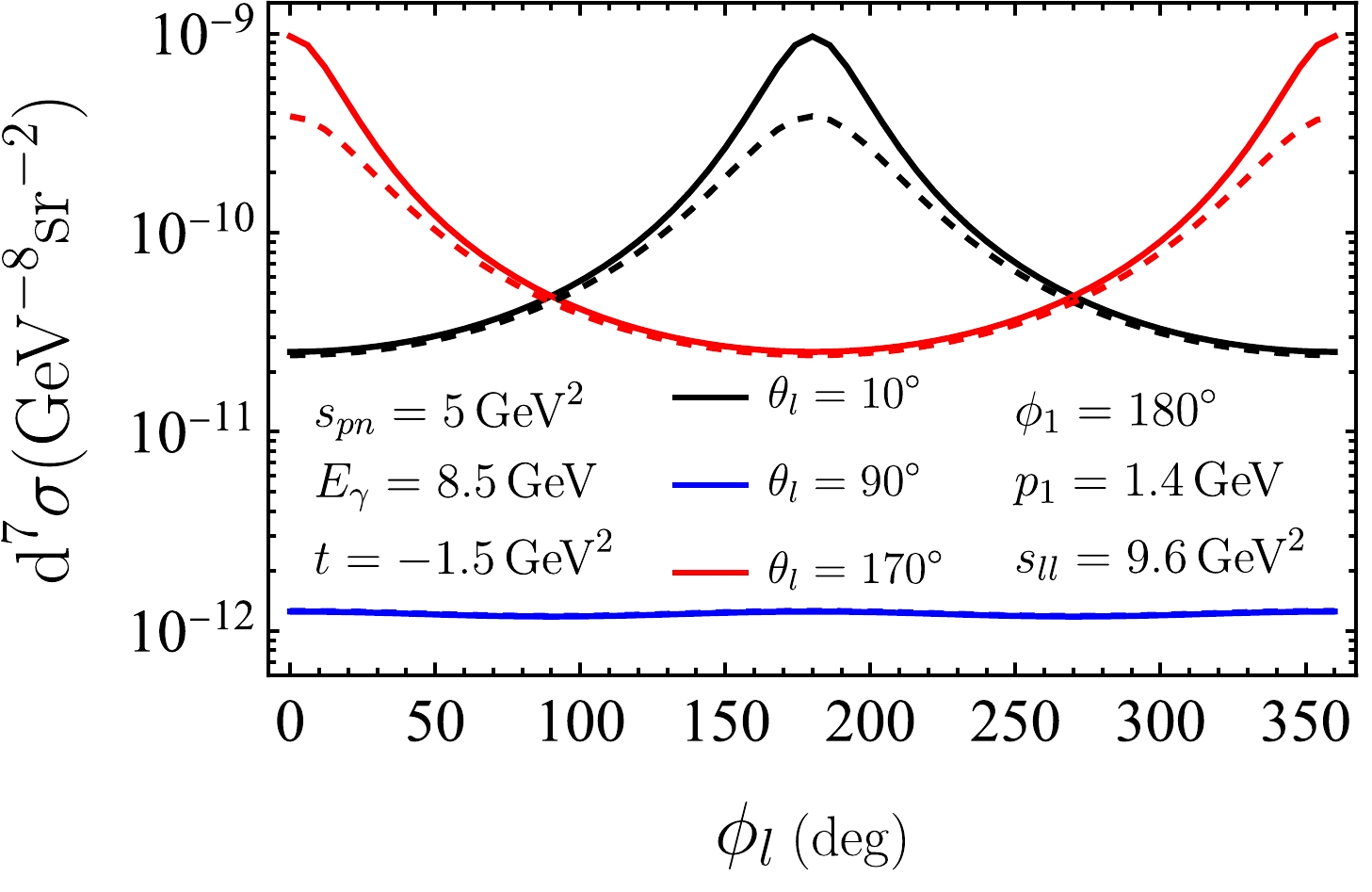
Figure 5. (color online) Differential cross sections of
$ e^+e^- $ production (solid curves) and$ \mu^+\mu^- $ production (dashed curves) in the PWIA as a function of$ \phi_l $ at$ E_\gamma=8.5\; {\rm{GeV}} $ ,$ s_{pn}=5\; {\rm{GeV}}^2 $ ,$ s_{ll}=9.6\; {\rm{GeV}}^2 $ ,$ t=-1.5\; {\rm{GeV}}^2 $ ,$ p_1=1.4\; {\rm{GeV}} $ ,$ \phi_1=180^\circ $ , and$ \theta_l=10^\circ,\,90^\circ,\,170^\circ $ , respectively. Label$ d^7 \sigma $ is a short-handed notation representing the seven-fold differential cross section$ {\rm d}^7\sigma / {{\rm{d}}} \Omega_p {{\rm{d}}} \Omega_{ll}{{\rm{d}}}s_{ll}{{\rm{d}}}s_{pn}{{\rm{d}}}t $ . The same notation is used in following figures.In Fig. 6, we plot the differential cross section as a function of
$ \phi_1 $ , the azimuthal angle of the proton. Furthermore,$ s_{ll} $ ,$ s_{pn} $ , and t are set at the same values as Fig. 5, and$ \theta_l=30^\circ $ and$ \phi_l = 180^\circ $ are fixed for the lepton angle. Given that the proton acquires the large momentum from the virtual photon, which has opposite transverse momentum to the lepton pair, the struck proton tends to be approximately$ \phi_1 = 180^\circ $ . In PWIA, the smearing is caused by the fermi motion, while FSI further broadens the distribution.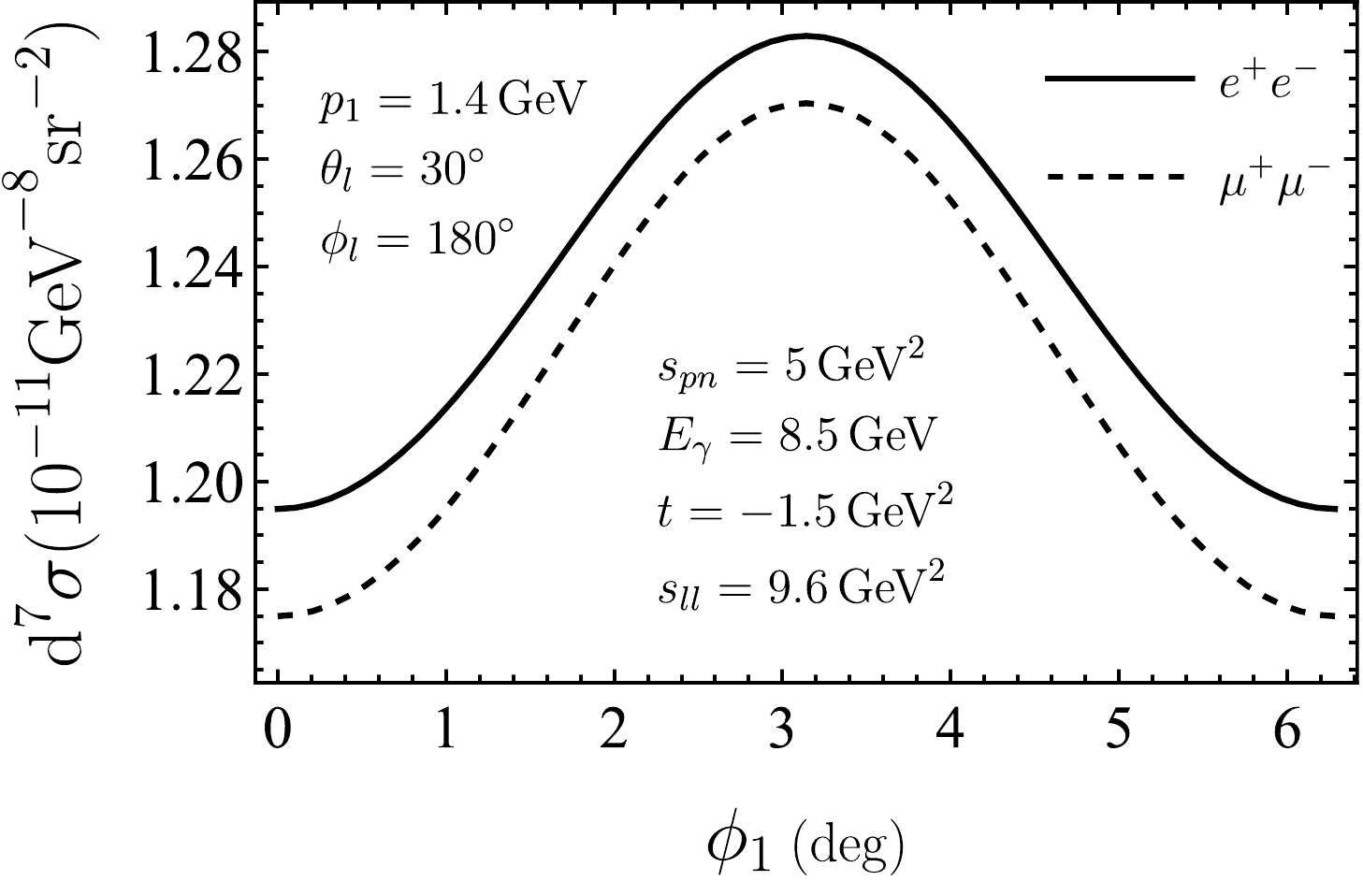
Figure 6. Differential cross sections of
$ e^+e^- $ production (solid curve) and$ \mu^+\mu^- $ production (dashed curve) in the PWIA as a function of$ \phi_1 $ at$ p_1=1.4\; {\rm{GeV}} $ ,$ \theta_l=30^\circ $ ,$ \phi_l=180^\circ $ , and the same$ E_\gamma $ ,$ s_{pn} $ ,$ s_{ll} $ , and t values as those in Fig. 5. -
For massless leptons, the differential cross section exhibits singularities if the lepton or the antilepton is collinear to the incident photon. This behavior is convenient to be understood from the BH amplitude. When the lepton is collinear to the photon, the lepton propagator in Fig. 2(a) approaches the pole. Similarly, the propagator in Fig. 2(b) reaches the pole when the antilepton is collinear to the photon. Such singularities are physically regularized by the lepton mass, which is maintained as nonzero in our calculation. However, a sharp peak is still observed for
$ e^+e^- $ production because of the tiny mass of the electron in comparison with typical scales of the reaction presented here.According to the physical origin of the singular behavior, it is straightforward to examine the differential cross section as a function of the lepton polar angle with respect to the incident photon. However, it is not a commonly used variable in describing the lepton pair production in deuteron breakup process. The singular behavior should be tracked from the dependence on other kinematic variables.
In Fig. 7, we plot the differential cross section as a function of
$ s_{ll} $ , with other kinematic variables set at$s_{pn} = 4.9~\rm GeV^2$ ,$t = -1.5~\rm GeV^2$ ,$p_1 = 1.3~\rm GeV$ ,$ \phi_1 = 180^\circ $ ,$ \theta_l = 15^\circ $ , and$ \phi_l = 180^\circ $ . One can observe that the cross section for$ e^+e^- $ production sharply peaks at approximately$ s_{ll}=9.15\,{\rm{GeV}}^2 $ , where the electron is collinear to the incident photon. To clearly observe this correspondence, we first examine the polar angle$ \theta_{34} $ of the lepton pair momentum$ {\boldsymbol{p}}_{34} $ . At fixed$ s_{pn} $ and t,$ \theta_{34} $ can be expressed as a function of$ s_{ll} $ . Their relation at the chosen kinematics is illustrated in Fig. 8. Then, we consider the direction of the electron in the lab frame. The lepton-photon collinear configuration occurs when$ \phi_e = 180^\circ $ and$ \theta_e^{\rm Lab} = \theta_{34} $ , where$ \theta_e^{\rm Lab} $ denotes the relative angle between the electron momentum$ {{{\boldsymbol{p}}}}_3 $ and lepton pair momentum$ {{{\boldsymbol{p}}}}_{34} $ in the laboratory frame. Based on the relation between$ \theta_e^{\rm Lab} $ and$ s_{ll} $ illustrated in Fig. 8, we can find the intersecting point, which indicates$ \theta_e^{\rm Lab} = \theta_{34} $ . The corresponding$ s_{ll} $ value is just at$ 9.15\,\rm GeV^2 $ . According to the definition of angles in Fig. 1, the positron-photon collinear configuration will occur at$ \phi_l = 0^\circ $ , and it can be analyzed via the same procedure. Given that muon is much heavier, the cross section of$ \mu^+\mu^- $ production does not show a sharp peak.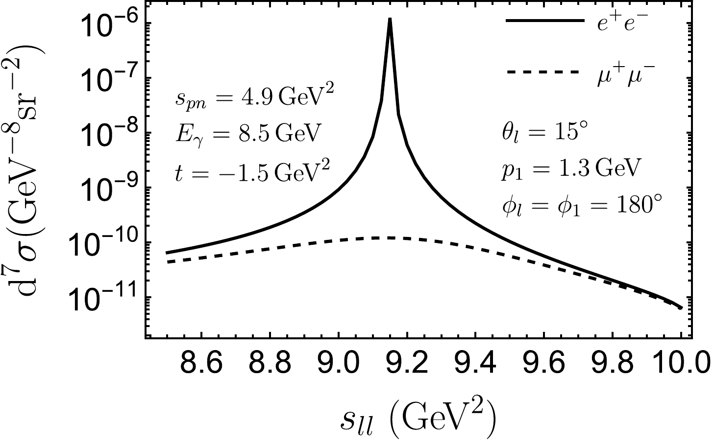
Figure 7. Differential cross sections for
$ e^+e^- $ production (solid line) and$ \mu^+\mu^- $ production (dashed line) in the PWIA as a function of$ s_{ll} $ at$ E_\gamma=8.5\; {\rm{GeV}} $ ,$ s_{pn}=4.9\; {\rm{GeV}}^2 $ ,$ t=-1.5\; {\rm{GeV}}^2 $ ,$ p_1=1.3\; {\rm{GeV}} $ ,$ \theta_l=15^\circ $ , and$ \phi_l=\phi_1=180^\circ $ .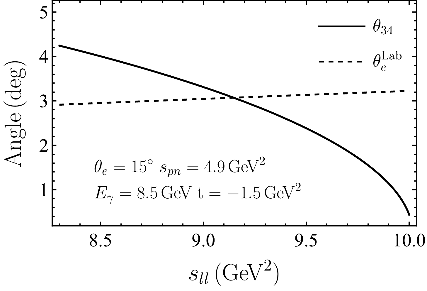
Figure 8.
$ \theta_{34} $ (solid line) and$ \theta_e^{{\rm{Lab}}} $ (dashed line) vary with$ s_{ll} $ at$ E_\gamma=8.5\; {\rm{GeV}} $ ,$ s_{pn}=4.9\; {\rm{GeV}}^2 $ , and$ t=-1.5\; {\rm{GeV}}^2 $ .Similarly, a sharp peak behavior can be observed in the dependence on other variables. In Fig. 9, we plot the differential cross section as a function of
$ s_{pn} $ , the invariant mass of the final proton-neutron system, while the other variables are set at$ s_{ll}=9~{\rm{GeV^2}} $ ,$ t=-2~{\rm{GeV}}^2 $ ,$ p_1=1.6~{\rm{GeV}} $ ,$ \theta_l=15^\circ $ ,$ \phi_l=180^\circ $ , and$ \phi_1=180^\circ $ . The cross section for$ e^+e^- $ productions peaks around$ s_{pn} = 5.7\,\rm GeV^2 $ .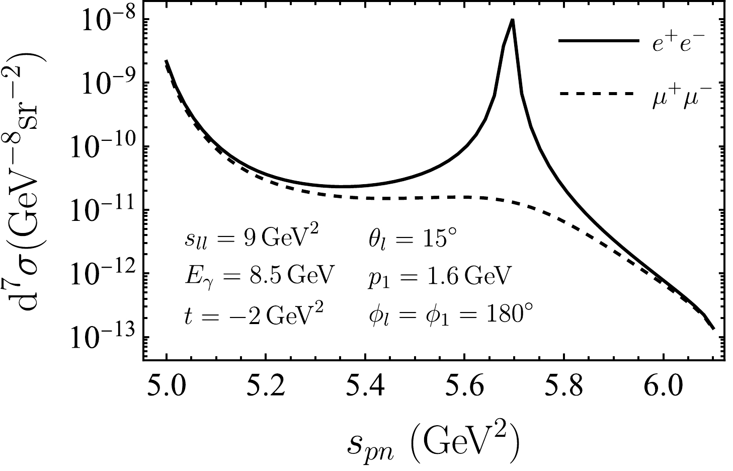
Figure 9. Differential cross sections for
$ e^+e^- $ production (dashed line) and$ \mu^+\mu^- $ production (dashed line) in the PWIA as a function of$ s_{pn} $ at$ E_\gamma=8.5\; {\rm{GeV}} $ ,$ s_{ll}=9\; {\rm{GeV^2}} $ ,$ t=-2\; {\rm{GeV}}^2 $ ,$ p_1=1.6\; {\rm{GeV}} $ ,$ \theta_l=15^\circ $ , and$ \phi_l=\phi_1=180^\circ $ .We note that the peak position in
$ s_{ll} $ or$ s_{pn} $ shifts to smaller values with increasing$ \theta_l $ . When$ \theta_l $ is sufficiently large, the momenta of the lepton and antilepton always diverge from the direction of the incident photon, and thus the differential cross section exhibits smooth behavior as a function of$ s_{pn} $ or$ s_{ll} $ as shown in Figs. 10 and 11.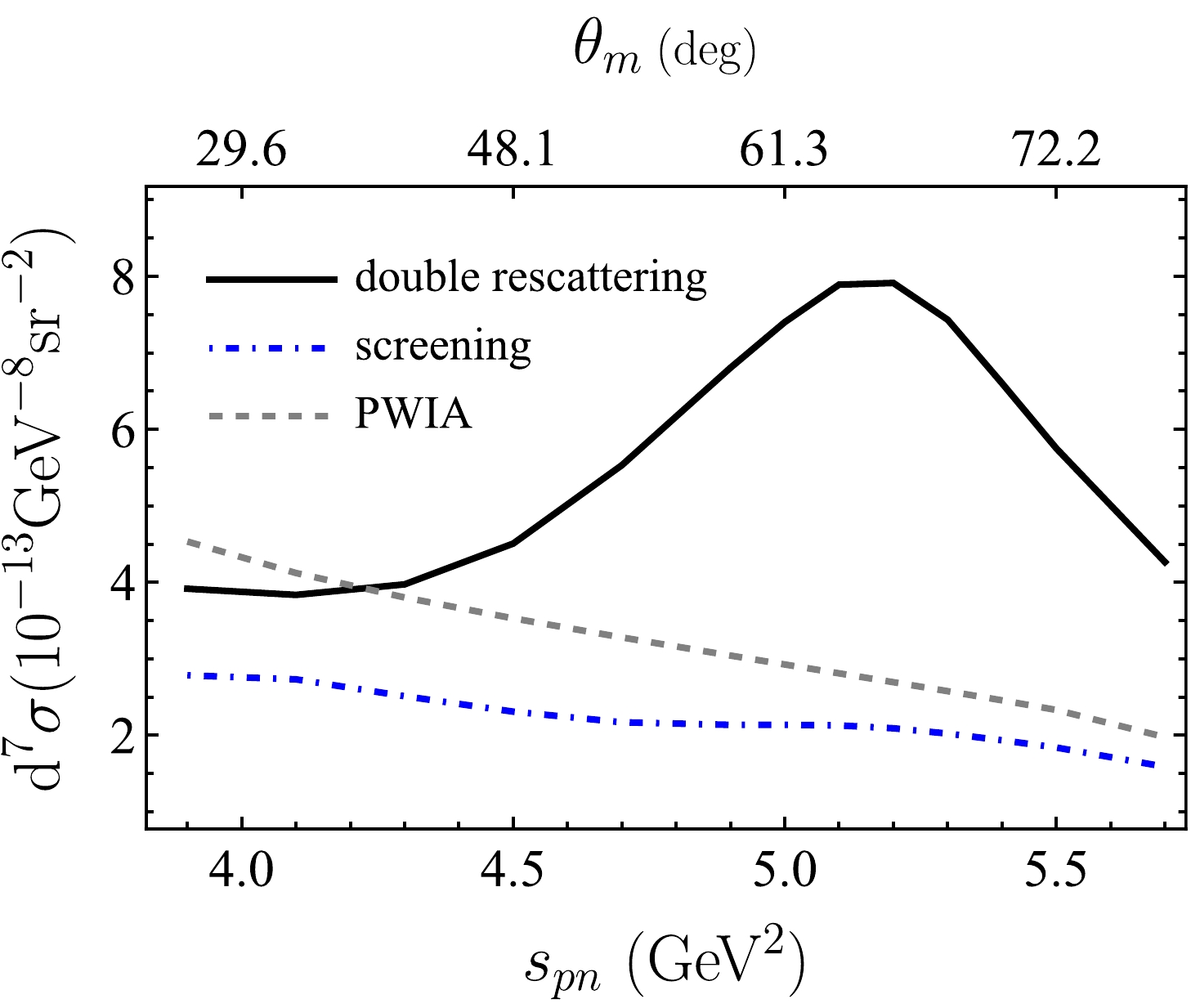
Figure 10. (color online) Differential cross sections for
$ e^+e^- $ production as a function of$ s_{pn} $ at$ E_\gamma=8.5\; {\rm{GeV}} $ ,$ t=-1.7\; {\rm{GeV}}^2 $ ,$ s_{ll}=9\; {\rm{GeV}}^2 $ ,$ p_m=0.45\; {\rm{GeV}} $ ,$ \phi_1=180^\circ $ ,$ \theta_e=60^\circ $ , and$ \phi_e=90^\circ $ in the PWIA (gray dashed curve), including the interference between the PWIA and FSI amplitudes (blue dot-dashed curve) and including both the interference term and the FSI amplitude square (black solid curve). Specifically,$ \theta_m $ axis is nonlinear.
Figure 11. (color online) Differential cross sections for
$ e^+e^- $ production as a function of$ s_{ll} $ at$ E_\gamma=8.5\; {\rm{GeV}} $ ,$ s_{pn}=4.9\; {\rm{GeV}}^2 $ ,$ t=-1.5\; {\rm{GeV}}^2 $ ,$ p_1=1.3\; {\rm{GeV}} $ ,$ \theta_e=40^\circ $ , and$ \phi_1=\phi_e=180^\circ $ . The gray dashed curve represents the result with PWIA, the black solid curve represents the result including the on-shell FSI, and the red dot-dashed curve represents the result including the on-shell and off-shell FSIs. -
In this subsection, we discuss the FSI contribution to the differential cross section. Given that the FSI effects on the
$ \mu^+\mu^- $ and$ e^+e^- $ productions are similar, we only present the results for$ e^+e^- $ production.In the PWIA, the reaction is approximated as the scattering from a quasi-free nucleon. As a general feature, the differential cross section decreases with increasing
$ |t| $ . To explore the deviation from the quasi-free picture, it is convenient to introduce the Bjorken variable$ x= Q^2/(2m\nu) $ , which approaches$ 1 $ for elastic scattering from a free nucleon. In Fig. 12, we show the phase space in$ s_{pn}-t $ plane together with lines indicating corresponding x values. With fixed$ s_{pn} $ , x becomes closer to$ 1 $ as$ |t| $ decreases, which implies that it is closer to the quasi-free kinematics.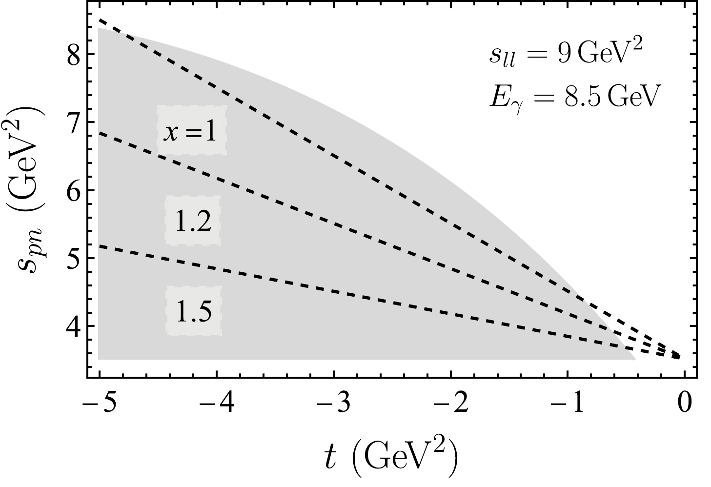
Figure 12.
$ s_{pn}-t $ phase space region at$ E_\gamma=8.5\; {\rm{GeV}} $ and$ s_{ll}=9\; {\rm{GeV}}^2 $ . The allowed kinematic range for t is larger than that plotted in the figure. Dashed lines show the Bjorken x at several fixed values.In Fig. 13, we plot the differential cross section as a function of t with other variables fixed at
$s_{pn}=5.1~{\rm{GeV}}^2$ ,$ s_{ll}=9~{\rm{GeV}}^2 $ ,$ p_1=1.45~{\rm{GeV}} $ ,$ \theta_e=60^\circ $ ,$ \phi_e=90^\circ $ , and$ \phi_1=180^\circ $ . Instead of showing the cross section in the full t region, we only present the result in the range of$ -3.5~{\rm GeV} < t < -1.5~{\rm GeV} $ . As described in Sec.II.B, we only consider the contribution from NN scattering in dealing with FSI. The meson exchange current (MEC) and isobar current (IC) contributions are neglected. As a conservative estimation, the MEC amplitude will have an overall additional$ \sim 1/(1+|t|/\Lambda^2)^2 $ dependence when compared to the IA amplitude where$ \Lambda^2 \sim 0.8-1\; \mathrm{GeV}^2 $ and IC amplitude will have at least an extra factor of$ 1/\sqrt{|t|} $ when compared with the elastic NN scattering amplitude [72]. Hence, both contributions are suppressed in large$ |t| $ kinematic region. Furthermore, for very large$ |t| $ , e.g.$ |t| > 5~\rm GeV^2 $ , the color coherence phenomena will complicate the situation [72−74]. Therefore we limit the value of t within a reasonable range for the current calculation. The dashed curve represents the result from PWIA, the solid curve represents the result including the on-shell FSI contribution, and the dot-dashed curve represents the result including the on-shell and off-shell FSI contributions. As observed in Fig. 13, the full FSI curve and on-shell FSI curve exhibit a slight difference when$ |t| $ is relatively small. This can be understood from Fig. 12, where it can be observed that the x becomes closer to$ 1 $ as$ |t| $ decreases with respect to fixed$ s_{pn} $ . At this limit, the kinematics is close to the quasi-free scattering and thus the off-shell FSI has little impact on the cross section.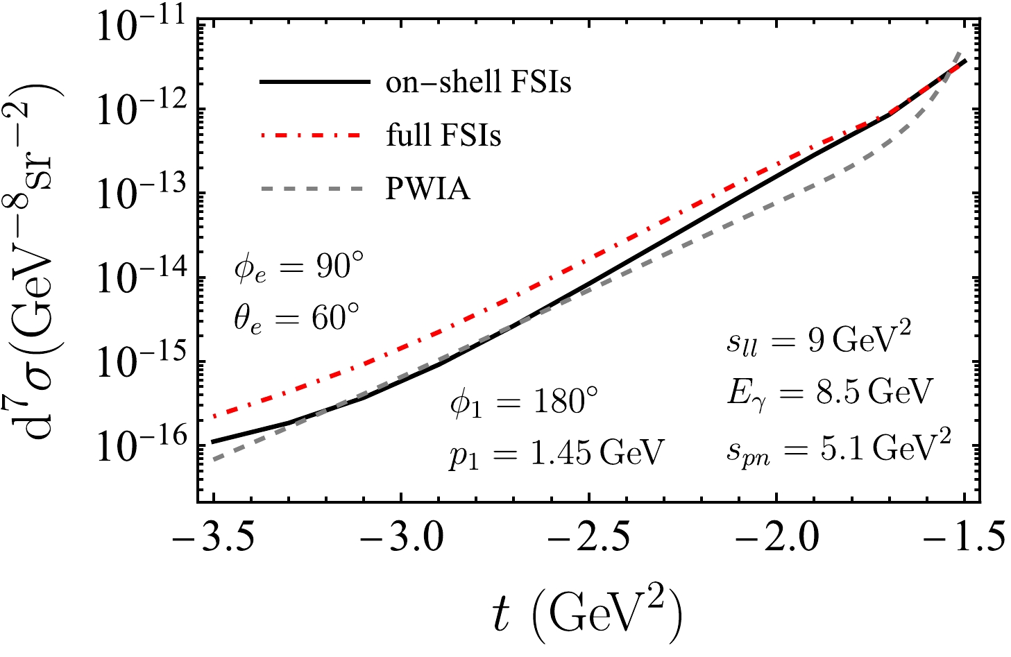
Figure 13. (color online) Differential cross sections for
$ e^+e^- $ production as a function of t at$ E_\gamma=8.5\; {\rm{GeV}} $ ,$ s_{pn}=5.1\; {\rm{GeV}}^2 $ ,$ s_{ll}=9\; {\rm{GeV}}^2 $ ,$ p_1=1.45\; {\rm{GeV}} $ ,$ \theta_e=60^\circ $ ,$ \phi_e=90^\circ $ , and$ \phi_1=180^\circ $ in three cases: in the PWIA (gray dashed curve), including the on-shell FSI (black solid curve), and including both the on-shell and off-shell FSIs (red dot-dashed curve).In Fig. 14, we plot the differential cross section as a function of the missing momentum
$ p_m $ , which is the amplitude of the momentum of the undetected nucleon. In the PWIA, the proton is knocked out by the virtual photon and acquires large momentum, while the spectator neutron carries relatively low momentum. Once the FSI is considered, the undetected neutron may receive momentum transfer via the NN scattering. Therefore, one may expect that the FSI effect is more significant in the region of relatively large$ p_m $ . This intuitive picture is confirmed by the numerical results in Fig. 14. The three curves are almost indistinguishable at small$ p_m $ , e.g., when$ p_m < 0.1\,\rm GeV $ . In this region, the FSI effect is a small quantity in comparison with the PWIA results. Hence, the PWIA is still a suitable approximation for the BH cross section. In contrast, in the large$ p_m $ region, e.g.,$ p_m > 0.4\,\rm GeV $ , a significant enhancement is caused by the FSI effects. It is also interesting to find that, in the medium$ p_m $ region,$ 0.1\,{\rm GeV} < p_m < 0.3\,\rm GeV $ , the cross section results including the FSI are less than the PWIA result, in which the suppression is from the interference between the PWIA amplitude and FSI amplitude. Furthermore, one may find that the full FSI curve and on-shell FSI curve exhibit slight difference in Fig. 14. This is attributed to the specific kinematics that result in x being close to 1, namely the quasi-free region, where the contribution from off-shell FSI is considerably small, as previously discussed.
Figure 14. (color online) Differential cross sections for
$ e^+e^- $ production as a function of the missing momentum$ p_m $ at$ E_\gamma=8.5\; {\rm{GeV}} $ ,$ s_{pn}=5.5\; {\rm{GeV}}^2 $ ,$ t=-2\; {\rm{GeV}}^2 $ ,$ s_{ll}=m_{J/\psi}^2 $ ,$ \theta_e=5^\circ $ , and$ \phi_e=\phi_1=180^\circ $ . The gray dashed curve represents the result with PWIA, the black solid curve represents the result including the on-shell FSI, and the red dot-dashed curve represents the result including both the on-shell and off-shell FSIs.In Fig. 15, we plot the differential cross section as a function of
$ \phi_1 $ with other variables fixed at$s_{pn}=5.5 {\rm{GeV}}^2$ ,$ t=-2\,{\rm GeV}^2 $ ,$ s_{ll}=m_{J/\psi}^2 $ ,$p_1=1.75~{\rm{GeV}}$ ,$ \phi_e=180^\circ $ , and$ \theta_e=45^\circ $ . The final-state proton momentum$ p_1=1.75 {\rm{GeV}} $ corresponds to the missing momentum$p_m = 0.152 {\rm{GeV}}$ , which is in the region where the FSI effects suppress the cross section. The on-shell FSI curve is slightly above the full FSI curve in the entire$ \phi_1 $ range.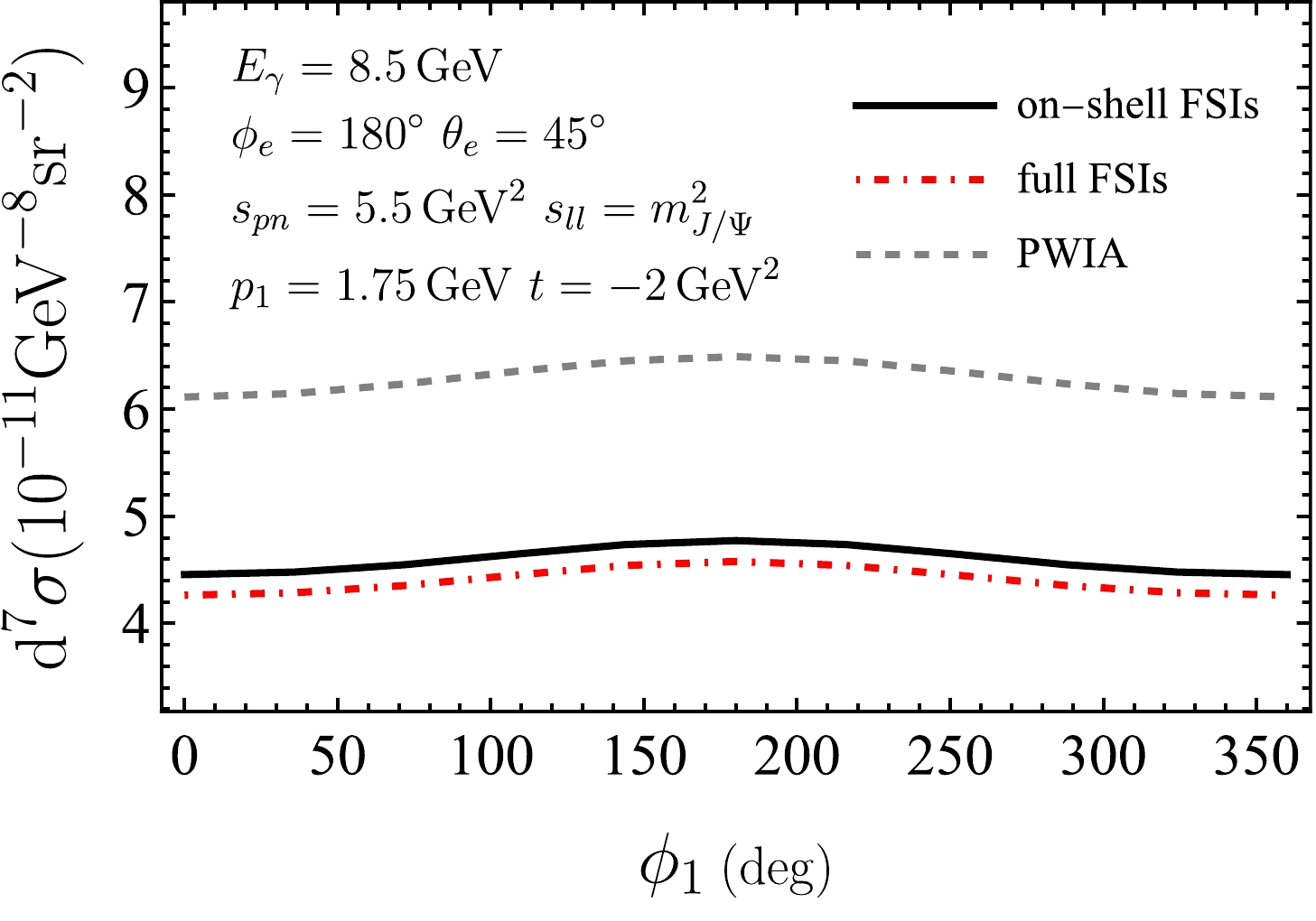
Figure 15. (color online) Differential cross sections for
$ e^+e^- $ production as a function of$ \phi_1 $ at$ E_\gamma=8.5\; {\rm{GeV}} $ ,$ s_{pn}=5.5\; {\rm{GeV}}^2 $ ,$ t=-2\; {\rm{GeV}}^2 $ ,$ s_{ll}=m_{J/\psi}^2 $ ,$ p_1=1.75\; {\rm{GeV}} $ ,$ \phi_e=180^\circ $ , and$ \theta_e=45^\circ $ . The gray dashed curve represents the result with PWIA, the black solid curve represents the result including the on-shell FSI, and the red dot-dashed curve represents the result including both the on-shell and off-shell FSIs.To clearly observe the contribution from the PWIA and FSI interference term and that from the FSI amplitude square term separately, we plot the differential cross section as a function of
$ s_{pn} $ with other variables fixed at$ t=-1.7\; {\rm{GeV}}^2 $ ,$ s_{ll}=9\; {\rm{GeV}}^2 $ ,$ \phi_1=180^\circ $ ,$ \theta_e=60^\circ $ , and$ \phi_e=90^\circ $ in Fig. 10, where the dashed curve represents the result with PWIA, the dot-dashed curve includes the interference term between PWIA and FSI amplitudes, and the solid curve includes both the interference term and FSI amplitude square term. For the numerical results in Fig. 10, FSI amplitude contains both on-shell and off-shell contributions. As observed, the interference term generally suppresses the cross section. For a chosen missing momentum, e.g.$ p_m=0.45\; {\rm{GeV}} $ , there exists a relation between the polar angle of the missing momentum with respect to the virtual photon,$ \theta_m $ , and$ s_{pn} $ , as marked on the top and bottom axes in Fig. 10. At forward angles of the missing momentum, the interference term dominates the FSI effects, leading to a suppression of the cross section compared with the PWIA result, even when both the interference term and the FSI amplitude square term are included. However, when$ \theta_m $ is large, which is more likely to be caused by the NN rescattering effects, the differential cross section is enhanced by the FSI and reaches a peak at approximately$ \theta_m \sim 65^\circ $ for the particular kinematic choice in Fig. 10. This is consistent with the typical FSI effects, as mentioned in Refs. [42, 45, 54, 72]. Specifically, the recoil nucleon receives transverse momentum via the rescattering while the knocked-out nucleon tends to eject away from the forward direction.In Fig. 11, we plot the cross section as a function of
$ s_{ll} $ with other variables fixed at$ s_{pn}=4.9\; {\rm{GeV}}^2 $ ,$ t=-1.5\; {\rm{GeV}}^2 $ ,$ p_1=1.3\; {\rm{GeV}} $ ,$ \theta_e=40^\circ $ , and$ \phi_1=\phi_e=180^\circ $ . As discussed in Sec. III.B, at large$ \theta_e $ , e.g.,$ \theta_e=40^\circ $ , the lepton momentum is away from the photon collinear direction. Hence, a sharp peak is absent in the$ s_{ll} $ dependence for this particular kinematic choice. Furthermore, FSI enhances the differential cross section but does not distort the trend of the curve in this case. -
For the reaction of deuteron disintegration, as shown in Fig. 4, the virtual photon can either couple to the proton or couple to the neutron. In principle, we should add the two possibilities at the amplitude level and then there is an interference term between the proton amplitude and neutron amplitude. However, this type of contribution is highly suppressed at certain kinematics as considered in this study.
In the PWIA, the nucleon struck by the virtual photon gains large momentum, while the spectator nucleon receives the Fermi motion momentum, which typically does not exceed several hundred MeV. When a high momentum nucleon, presumably the proton, is detected in the final state, it is likely the one that interacted with the virtual photon. However, once FSIs are considered, it is possible that the detected high momentum nucleon does not directly interact with the virtual photon but rather obtains its high momentum via nucleon-nucleon (NN) scattering. In such scenarios, we must assess whether the interference contribution remains negligible. Under the assumption of isospin symmetry, the matrix element of the electromagnetic current operator can be expressed as
$ J^\mu(q)_{{\rm{if}}}=\frac{1}{\sqrt{2}}\left(J_p^\mu(q)_{{\rm{if}}}-J_n^\mu(q)_{{\rm{if}}}\right) \; , $

(36) where subscript
$ N = p,n $ indicates the nucleon, which absorbs the virtual photon. Then, the interference term for the nuclear tensor is$ W_{{\rm{interf}}}^{\mu\nu}=-(2m)^2\overline{\sum\limits_{{\rm{if}}}}\frac{1}{2}\left(J_p^\mu(q)_{{\rm{if}}} J_n^{\nu\,\dagger}(q)_{{\rm{if}}}+J_n^\mu(q)_{{\rm{if}}} J_p^{\nu\,\dagger}(q)_{{\rm{if}}}\right)\; . $

(37) In Fig. 16, we compare the differential cross section with and without the interference term between the proton amplitude and neutron amplitude in the range of the missing momentum from
$ 0 $ to$ 0.8\,\rm GeV $ . The gray dashed and blue dotted curves represent the results with and without the interference term in the PWIA, respectively. The black solid and red dashed curves represent the results with and without the interference term including FSI effects, respectively. Furthermore, no visible difference is observed in either case.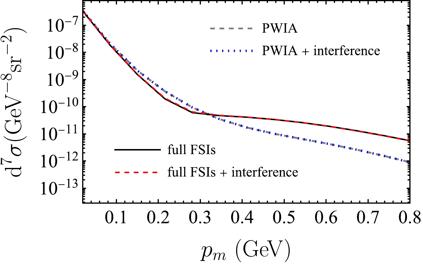
Figure 16. (color online) Differential cross sections with and without the interference term between the proton and neutron amplitudes. The results are drawn at
$ E_\gamma=8.5\; {\rm{GeV}} $ ,$ s_{pn}=5.5\; {\rm{GeV}}^2 $ ,$ t=-2\; {\rm{GeV}}^2 $ ,$ s_{ll}=m_{J/\psi}^2 $ ,$ \theta_e=5^\circ $ , and$\phi_e=\phi_1= $ $ 180^\circ$ . -
In this study, we investigate lepton pair production during the deuteron breakup reaction. Our analysis includes a calculation of the complete seven-fold differential cross section, focusing on lepton pairs generated via the Bethe-Heitler mechanism. The bound state of the deuteron is characterized using a relativistic covariant deuteron-nucleon vertex. Within this framework, the form factors are represented as linear combinations of deuteron wave functions, which are solutions to the Gross equation [49]. In addition to the PWIA calculations, we incorporate FSI, resulting from the rescattering between the knocked-out nucleon and spectator nucleon. The NN scattering amplitude is parameterized in a Lorentz covariant form, encompassing all spin-dependent contributions. The parameterization functions are derived from the partial wave expansion formalism.
Furthermore, we conduct numerical calculations. The differential cross section can vary by orders of magnitude in dependence on the lepton azimuthal angle
$ \phi_l $ when the polar angle$ \theta_l $ approaches$ 0^\circ $ or$ 180^\circ $ . However, for the middle polar angle, the azimuthal angle dependence is mild. In$ s_{ll} $ and$ s_{pn} $ dependence, sharp peaks are also observed. These nearly singular behaviors stem from the collinear singularity for massless leptons, occurring when the lepton or antilepton moves along the direction of the incident photon. In the specific kinematics examined in this study, the produced lepton pair moves at a forward angle, preventing the appearance of a sharp peak when the lepton's polar angle is near the vertical. This singularity is physically regularized in our calculations by considering the lepton mass. Numerically, we observe that the differential cross section for$ \mu^+\mu^- $ production is much smoother than that for$ e^+e^- $ due to the heavier mass.The FSI effects exhibit strong dependence on the missing momentum
$ p_m $ because the recoil nucleon can receive energy-momentum transfer in the rescattering. When the missing momentum is relatively small, the FSI contribution is negligible, and the PWIA provides a good approximation of the full result. While the missing momentum is large, the FSI leads to significant enhancement of the differential cross section. In the intermediate missing momentum region, we observe a suppression of the cross section due to the interference between the PWIA amplitude and FSI amplitude. By dividing the FSI contribution into on-shell and off-shell parts, we discover that the on-shell term predominates in a relatively small$ |t| $ region in which Bjorken x approaches 1, the quasi-elastic limit. When x is away from$ 1 $ , corresponding to large$ |t| $ region, the off-shell term dominates the FSI effect. Furthermore, we investigate the contribution from the interference between the proton amplitude and neutron amplitude. With explicit numerical calculation, we demonstrate that this contribution is negligible in the kinematics region considered in this study, even if the FSI effects are considered.The dilepton production in the deuteron breakup process serves as an important input in the analysis of
$ J/\psi $ production, DVMP, and TCS measurements using a deuteron target or beam. The interference term between TCS and BH amplitudes can be singled out from the experiment data via the so-called forward-backword (FB) asymmetry [31, 36]. It could act as an amplifier for the TCS process and provide access to the Compton form factors in a linear form. When FSI is included, both the real and imaginary parts of Compton form factors will contribute and couple with the scalar functions$ F_j(s_N,t_N) $ that describe NN scattering. Therefore, careful consideration of the FSI effect is essential when extracting GPDs from processes involving the deuteron. The treatment of FSIs is particularly important for the accurate subtraction of BH background in the photoproduction of$ J/\psi $ on the deuteron because the FSI effect will be dominant at the relatively large missing momentum. Consequently, this process holds significant relevance for the physics program at Jefferson Lab and future electron-ion colliders. -
We are grateful to Ron L. Workman and Igor I. Strakovsky for sending us the SAID manual that contains information on the nucleon-nucleon amplitudes. We thank Haiyan Gao, Gregory Matousek, Richard Tyson, and Zhiwen Zhao for helpful discussions.
-
The four body phase space can be expressed as
$ \begin{aligned}[b] \int \mathrm{d} \Pi=& \int (2\pi)^{4} \delta^{(4)}(k+P-p_1-p_2-p_3-p_4)\\& \times\frac{\mathrm{d}^3 {\boldsymbol{p}}_1}{(2\pi)^3 2 E_1} \frac{\mathrm{d}^3 {\boldsymbol{p}}_2}{(2\pi)^3 2 E_2} \frac{\mathrm{d}^3 {\boldsymbol{p}}_3}{(2\pi)^3 2 E_3} \frac{\mathrm{d}^3 {\boldsymbol{p}}_4}{(2\pi)^3 2 E_4}\; . \end{aligned}\tag{A1} $

To separate the phase space for the lepton pair part and nuclear part, the following delta function integration can be inserted as follows:
$ \begin{aligned}[b]& \int \frac{\mathrm{d}^4 p_{34}}{(2\pi)^4} \,(2\pi)^4 \,\delta^{(4)}(p_{34}-p_3-p_4) \int \frac{\mathrm{d}s_{ll}}{2\pi} \,2\pi\, \delta(s_{ll}-p_{34}^2)\\ =&\int\frac{\mathrm{d}s_{ll}}{2\pi}\int \frac{\mathrm{d}^3 {\boldsymbol{p}}_{34}}{(2\pi)^3 2E_{34}}\,(2\pi)^4\, \delta^{(4)}(p_{34}-p_3-p_4)\; . \end{aligned}\tag{A2} $

Where
$ p^0_{34}=E_{34}=\sqrt{|{\boldsymbol{p}}_{34}|^2+s_{ll}} $ . Then, the phase space can be expressed as follows:$ \begin{aligned}[b] \int \mathrm{d} \Pi =& \int\frac{\mathrm{d}s_{ll}}{2\pi} (2\pi)^4 \delta^{(4)}(k+P-p_1-p_2-p_{34})\\& \times\frac{\mathrm{d}^3 {\boldsymbol{p}}_1}{(2\pi)^3 2 E_1} \frac{\mathrm{d}^3 {\boldsymbol{p}}_2}{(2\pi)^3 2 E_2} \frac{\mathrm{d}^3 {\boldsymbol{p}}_{34}}{(2\pi)^3 2E_{34}} \\ &\times (2\pi)^4 \,\delta^{(4)}(p_{34}-p_3-p_4) \\& \times\frac{\mathrm{d}^3 {\boldsymbol{p}}_3}{(2\pi)^3 2 E_3} \frac{\mathrm{d}^3 {\boldsymbol{p}}_4}{(2\pi)^3 2 E_4}\; . \end{aligned}\tag{A3} $

The phase space for lepton pair is calculated in the lepton pair center of mass frame,
$ \begin{aligned}[b] \mathrm{d}\Pi_{ll}=&\int (2\pi)^4 \,\delta^{(4)}(p_{34}-p_3-p_4)\\& \times\frac{\mathrm{d}^3 {\boldsymbol{p}}_3}{(2\pi)^3 2 E_3} \frac{\mathrm{d}^3 {\boldsymbol{p}}_4}{(2\pi)^3 2 E_4}\\ =&\int \frac{|{\boldsymbol{p}}_c|}{\sqrt{s_{ll}}}\frac{\mathrm{d} \Omega_{ll}}{(4\pi)^2}\; , \end{aligned}\tag{A4} $

in which
$ {\boldsymbol{p}}_c $ denotes the momenta of the lepton in the center of mass frame. The phase space for the proton and neutron is calculated in the laboratory system, in which z axis is along$ {\boldsymbol{q}} $ direction as follows:$ \begin{aligned}[b] \mathrm{d} \Pi_{pn}=&\int (2\pi)^4 \delta^{(4)}(k+P-p_1-p_2-p_{34})\\& \times\frac{\mathrm{d}^3 {\boldsymbol{p}}_1}{(2\pi)^3 2 E_1} \frac{\mathrm{d}^3 {\boldsymbol{p}}_2}{(2\pi)^3 2 E_2} \frac{\mathrm{d}^3 {\boldsymbol{p}}_{34}}{(2\pi)^3 2E_{34}}\\ =&\int \frac{1}{(2\pi)^5}\frac{|{\boldsymbol{p}}_1|^2}{8E_{34}}\frac{\mathrm{d}^3 |{\boldsymbol{p}}_{34}|\mathrm{d} \Omega_1}{||{\boldsymbol{p}}_1|(m_d+\nu)-E_1|{\boldsymbol{q}}|\cos \theta_1|}\; . \end{aligned} \tag{A5}$

where
$ {\boldsymbol{p}}_1 $ is determined by the following equation:$ m_d+\nu=\sqrt{m^2+|{\boldsymbol{p}}_1|^2}+\sqrt{m^2+|{\boldsymbol{p}}_1|^2+|{\boldsymbol{q}}|^2-2|{\boldsymbol{q}}||{\boldsymbol{p}}_1|\cos \theta_1}\; . \tag{A6}$

Using the following relations,
$ \begin{aligned}[b] s_{pn}=&t+2m_d\nu+m_d^2\; ,\\ |{\boldsymbol{p}}_{34}|=&\sqrt{(E_\gamma-\nu)^2-s_{ll}}\; ,\\ \cos\theta_{34}=&\frac{E_\gamma^2+(E_\gamma-\nu)^2-s_{ll}-(\nu^2-t)}{2E_\gamma\sqrt{(E_\gamma-\nu)^2-s_{ll}}}\; , \end{aligned}\tag{A7} $

we can perform transformation of variables from
$ s_{ll} $ ,$ |{\boldsymbol{p}}_{34}| $ , and$ \theta_{34} $ to$ s_{ll} $ ,$ s_{pn} $ , and t. Based on Eqs. (3) and (4), the differential cross section can be expressed:$ \begin{aligned}[b] {{{\rm{d}}}} \sigma =&\frac{\alpha^3}{8(4\pi)^4}\frac{|{\boldsymbol{p}}_1|^2\beta}{m_d^2 E_\gamma^2 t^2}\frac{L^{\mu\nu}W_{\mu\nu}}{||{\boldsymbol{p}}_1|(m_d+\nu)-E_1|{\boldsymbol{q}}|\cos \theta_1|}\\& \times {{\rm{d}}} \Omega_p {{\rm{d}}} \Omega_{ll}{{\rm{d}}}s_{ll}{{\rm{d}}}s_{pn}{{\rm{d}}}t\; . \end{aligned}\tag{A8} $

-
Realtions between four scalar invariant functions and deuteron wave functions in the deuteron rest frame are as follows:
$ \begin{aligned}[b] F({\boldsymbol{p}})=&\pi \sqrt{2 m_{d}}\left(2 E_{p}-m_{d}\right)\\& \times \left[u({\boldsymbol{p}})-\frac{1}{\sqrt{2}} w({\boldsymbol{p}})+\sqrt{\frac{3}{2}}\frac{m}{|{\boldsymbol{p}}|} v_{t}({\boldsymbol{p}})\right]\; , \end{aligned}\tag{B1} $

$ \begin{aligned}[b] G({\boldsymbol{p}})=&\pi m\sqrt{2 m_{d}}\left(2 E_{p}-m_{d}\right)\\& \times\left[\frac{ u({\boldsymbol{p}})}{E_{p}+m}+ \frac{\left(2 E_{p}+m\right)}{\sqrt{2}|{\boldsymbol{p}}|^{2}}w({\boldsymbol{p}})+\sqrt{\frac{3}{2}}\frac{1}{|{\boldsymbol{p}}|} v_{t}({\boldsymbol{p}})\right]\; , \end{aligned}\tag{B2} $

$ H({\boldsymbol{p}})=\pi \sqrt{3m_{d}} \frac{E_{p} m}{|{\boldsymbol{p}}|} v_{t}({\boldsymbol{p}})\; , \tag{B3} $

$ \begin{aligned}[b] I({\boldsymbol{p}})=&-\pi \frac{\sqrt{2}m^{2}}{\sqrt{m_{d}}}\Bigg[\left(2 E_{p}-m_{d}\right)\\& \times \left(\frac{u({\boldsymbol{p}})}{E_{p}+m}- \frac{E_{p}+2 m}{\sqrt{2}|{\boldsymbol{p}}|^2}w({\boldsymbol{p}})\right)+\sqrt{3}\frac{m_{d}}{|{\boldsymbol{p}}|} v_{s}({\boldsymbol{p}})\Bigg]\; , \end{aligned}\tag{B4} $

where
$ |{\boldsymbol{p}}|=\sqrt{\dfrac{(P\cdot k_2)^2}{P^2}-k_2^2} $ , P denotes the four-momentum of the deuteron and$ k_2 $ denotes the four-momentum of the on-shell nucleon. The derivation details can be found in Refs. [47, 52], and the normalization of wave functions is as follows:$ \int_0^\infty \left[u^2({\boldsymbol{p}})+w^2({\boldsymbol{p}})+v_t^2({\boldsymbol{p}})+v_s^2({\boldsymbol{p}})\right] |{\boldsymbol{p}}|^2 {{{\rm{d}}}} |{\boldsymbol{p}}| = 1\; . \tag{B5} $

In our calculation, numerical solutions for the deuteron wave functions
$ u({\boldsymbol{p}}) $ ,$ w({\boldsymbol{p}}) $ ,$ v_t({\boldsymbol{p}}) $ and$ v_s({\boldsymbol{p}}) $ are from Ref. [49]. -
We show construction details for the Dirac trace in Eq. (15) in this appendix. With Eq. (10),
$ W^{\mu\nu} $ can be expressed in the following form:$ \begin{aligned}[b] W^{\mu\nu}=&\frac{(2m)^2}{3}\sum\limits_{\lambda_d,s_1,s_2}\langle{\boldsymbol{p}}_{1} s_{1} ; {\boldsymbol{p}}_{2} s_{2}\left|\hat{J}^{\mu}\right| {\boldsymbol{P}} \lambda_{d}\rangle_{{\rm{PW}}}\langle {\boldsymbol{P}} \lambda_{d}\left|\hat{J}^{\nu\,\dagger}\right|{\boldsymbol{p}}_{1} s_{1} ; {\boldsymbol{p}}_{2} s_{2}\rangle_{{\rm{PW}}}\\ =&\frac{(2m)^2}{3}\sum\limits_{\lambda_d,s_1,s_2}\bar{u}\left({\boldsymbol{p}}_{1}, s_{1}\right) \Gamma_N^{\mu}(q) \frac{\not {P}-\not {p}_2+m}{m^2-(P-p_2)^2} \Gamma_{\lambda_{d}}\left(p_{2}, P\right)C \gamma^0 u^{*} \left({\boldsymbol{p}}_{2}, s_{2}\right)\\ &\times \bar{u}^{*} \left({\boldsymbol{p}}_{2}, s_{2}\right)C^\dagger \gamma^0 \tilde{\Gamma}_{\lambda_d}\frac{\not {P}-\not {p}_2+m}{m^2-(P-p_2)^2}\tilde{\Gamma}_N^\nu u\left({\boldsymbol{p}}_{1}, s_{1}\right)\; . \end{aligned}\tag{C1} $ 
It should be noted that
$ \gamma^0 \gamma^{\mu\,\dagger} \gamma^0=\gamma^\mu $ ,$ \gamma^0 \gamma^{\mu\,*} \gamma^0=\gamma^{\mu\,T} $ ,$ \gamma^0 C^\dagger \gamma^0 = -C^{-1} $ , and$ C \gamma^\mu C^{-1}= - \gamma^{\mu\,T} $ ,$ \sum\limits_{s_2} C \gamma^0 u^{*} \left({\boldsymbol{p}}_{2}, s_{2}\right) \bar{u}^{*} \left({\boldsymbol{p}}_{2}, s_{2}\right)C^\dagger \gamma^0=\frac{\not {p}_2-m}{2m}\; . \tag{C2} $

Hence, it follows that
$ \begin{aligned}[b]\\ W^{\mu\nu} =&{{\rm{Tr}}}\Bigg[\Gamma_N^{\mu}(q) \frac{\not {P}-\not {p}_2+m}{m^2-(P-p_2)^2} \Gamma_D^\alpha\left(p_{2}, P\right)\left(\not {p}_2-m\right)\\& \times \widetilde{\Gamma}_D^\beta\frac{\not {P}-\not {p}_2+m}{m^2-(P-p_2)^2}\widetilde{\Gamma}_N^\nu \left(\not {p}_1+m\right)\Bigg]\\ &\times \frac{1}{3}\sum\limits_{\lambda_d=1}^3 \xi_\alpha^{\lambda_d}(P)\; \xi^{*\,\lambda_d}_\beta(P)\; . \end{aligned}\tag{C3} $

-
Two ways of parameterization in Eqs. (19) and (20) for the nucleon nucleon scattering matrix can be related by the helicity amplitudes. Helicity amplitudes are defined by scattering amplitudes in which initial states and final states have specific helicities of
$ \lambda_i $ and$ \lambda^\prime_i $ , respectively:$ \begin{aligned}[b] \mathcal{M}_{\lambda_{1}^{\prime} \lambda_{2}^{\prime} ; \lambda_{1} \lambda_{2}} =&\bar{u}_{\alpha^\prime}\left({\boldsymbol{p}}_{1}^{\prime},\lambda_{1}^{\prime}\right)\bar{u}_{\beta^\prime}\left({\boldsymbol{p}}_{2}^{\prime},\lambda_{2}^{\prime}\right)\\& \times M_{\alpha^\prime \alpha, \beta^\prime \beta}\,u_{\alpha}\left({\boldsymbol{p}}_{1},\lambda_{1}\right)u_{\beta}\left({\boldsymbol{p}}_{2},\lambda_{2}\right), \end{aligned}\tag{D1} $

where α,
$ \alpha^\prime $ and β,$ \beta^\prime $ denote the Dirac indexes for the first and second particles, respectively. Furthermore,$ u\left({\boldsymbol{p}}_{i},\lambda_{i}\right) $ denotes the Dirac spinor with momentum$ {\boldsymbol{p}}_i $ and helicity$ \lambda_i $ , and it is defined as follows:$ u({\boldsymbol{p}}_i, \lambda)=N\begin{pmatrix} 1 \\ 2 \lambda \tilde{p}_i \end{pmatrix} | \lambda\rangle_i\; , \tag{D2} $

where
$ \tilde{p}=\dfrac{|{\boldsymbol{p}}|}{E_p+m} $ ,$ N=\sqrt{\dfrac{E_p+m}{2m}} $ , and$ E_p=\sqrt{m^2+{\boldsymbol{p}}^2} $ . Furthermore,$ |\lambda\rangle_i $ in the center of mass frame is listed in Table D1. We use the convention in Refs. [48, 49, 75].Initial state Final state $ \lambda=\dfrac{1}{2} $ 

$ \lambda=-\dfrac{1}{2} $ 

$ \lambda=\dfrac{1}{2} $ 

$ \lambda=-\dfrac{1}{2} $ 

$ |\lambda\rangle_1 $ 

$ \begin{pmatrix} 1\\ 0\end{pmatrix} $ 

$ \begin{pmatrix} 0\\ 1\end{pmatrix} $ 

$ |\lambda\rangle_1 $ 

$\left(\begin{aligned} \cos (\dfrac{1}{2} \theta)\\ \sin( \dfrac{1}{2} \theta) \end{aligned}\right)$ 

$\left(\begin{aligned} -\sin (\dfrac{1}{2} \theta)\\ \cos (\dfrac{1}{2} \theta)\end{aligned}\right)$ 

$ |\lambda\rangle_2 $ 

$ \begin{pmatrix} 0\\ 1\end{pmatrix} $ 

$ \begin{pmatrix} 1\\ 0\end{pmatrix} $ 

$ |\lambda\rangle_2 $ 

$\left(\begin{aligned} -\sin (\dfrac{1}{2} \theta)\\ \cos (\dfrac{1}{2} \theta)\end{aligned}\right)$ 

$\left(\begin{aligned} \cos (\dfrac{1}{2} \theta)\\ \sin (\dfrac{1}{2} \theta)\end{aligned}\right)$ 

Table D1.
$ |\lambda\rangle_i $ in Eq. (D2).Considering parity conservation, time reversal invariance, and the Pauli principle, there are five independent helicity amplitudes [66] as follows:
$ \begin{aligned}[b] M_{1} \equiv& \mathcal{M}_{\textstyle\frac{1}{2}\frac{1}{2};\frac{1}{2}\frac{1}{2}}\; ,\\ M_{2} \equiv& \mathcal{M}_{\textstyle\frac{1}{2}\frac{1}{2};-\frac{1}{2}-\frac{1}{2}}\; , \\ M_{3} \equiv& \mathcal{M}_{\textstyle\frac{1}{2}-\frac{1}{2};\frac{1}{2}-\frac{1}{2}}\; ,\\ M_{4} \equiv& \mathcal{M}_{\textstyle\frac{1}{2}-\frac{1}{2};-\frac{1}{2}\frac{1}{2}}\; , \\ M_{5} \equiv& \mathcal{M}_{\textstyle\frac{1}{2}\frac{1}{2};\frac{1}{2}-\frac{1}{2}}\; . \end{aligned}\tag{D3} $

Substituting Dirac spinors with specific helicities from Eq. (D2) and the parameterization Eq. (19) of
$ M_{\alpha^\prime \alpha, \beta^\prime \beta} $ into Eq. (D3) to calculate independent helicity amplitudes, we obtain the relations of$ M_1 $ ,$ M_2 $ ,$ M_3 $ ,$ M_4 $ , and$ M_5 $ with$ F_{S}(s_N, t_N) $ ,$ F_{V}(s_N, t_N) $ ,$ F_{T}(s_N, t_N) $ ,$ F_{P}(s_N, t_N) $ , and$ F_{A}(s_N, t_N) $ ,$ \begin{aligned}[b] M_1=&\frac{1}{2m^2}\left(m^2(\cos \theta+1)F_{S}+ (m^2+m^2\cos \theta +4 {\boldsymbol{p}}^2)F_{V}\right.\\ &+ \left. 2m^2(\cos \theta -3) F_{T}+(-m^2\cos \theta+3m^2+4{\boldsymbol{p}}^2)F_{A}\right)\; ,\\ M_2=&\frac{1}{2m^2}\left((\cos\theta -1)E_p^2F_{S}+ m^2(\cos\theta-1)F_{V}\right.\\ &+2(\cos \theta +3)(m^2+2{\boldsymbol{p}}^2)F_{T}+ {\boldsymbol{p}}^2(\cos\theta-1)F_{P} \\&-m^2(\cos \theta+3)F_{A})\; ,\\ M_3=& \frac{1}{m^2}\left(m^2\cos^2 \frac{\theta}{2}F_{S} +(m^2+2{\boldsymbol{p}}^2)\cos^2\frac{\theta}{2}F_{V}\right.\\ &+\left.2m^2\cos^2 \frac{\theta}{2}F_{T}-(m^2+2{\boldsymbol{p}}^2)\cos^2 \frac{\theta}{2}F_{A}\right)\; ,\\ M_4=&\frac{1}{m^2}\left(\sin^2\frac{\theta}{2}E_p^2F_{S}+m^2\sin^2\frac{\theta}{2}F_{V}\right.\\ &+\left.2m^2\sin^2\frac{\theta}{2}F_{T}-{\boldsymbol{p}}^2\sin^2\frac{\theta}{2}F_{P}-m^2\sin^2\frac{\theta}{2}F_{A}\right)\; ,\\ M_5=&\frac{E_p}{2m}\left(-\sin\theta F_{S} -\sin\theta F_{V} -2\sin\theta F_{T}+ \sin\theta F_{A}\right)\; . \end{aligned}\tag{D4}$

Relations of a, b, c, d, and e with helicity amplitudes
$ M_i^{\rm SAID} $ are provided in Ref. [66] and listed here for convenience,$ \begin{aligned}[b] M^{\rm SAID}_{1}=&\frac{1}{2}(a \cos \theta+b-c+d+{\rm i} e \sin \theta)\; , \\ M^{\rm SAID}_{2}=&\frac{1}{2}(a \cos \theta-b+c+d+{\rm i} e \sin \theta)\; , \\ M^{\rm SAID}_{3}=&\frac{1}{2}(a \cos \theta+b+c-d+{\rm i} e \sin \theta)\; , \\ M^{\rm SAID}_{4}=&\frac{1}{2}(-a \cos \theta+b+c+d-{\rm i} e \sin \theta)\; , \\ M^{\rm SAID}_{5}=&\frac{1}{2}(-a \sin \theta+{\rm i} e \cos \theta)\; . \end{aligned}\tag{D5} $

The partial wave expansion for amplitudes a, b, c, d, and e is discussed in Ref. [67]. Using the phase shift analysis of Refs. [68, 69] and phase shift data available from SAID program [70], we obtain the value of amplitudes at the specific momentum
$ |{\boldsymbol{p}}| $ and scattering angle θ. The unpolarized differential cross section in our convention is as follows:$ \frac{ {{{\rm{d}}}} \sigma}{ {{{\rm{d}}}} \Omega} = \frac{1}{4} \sum\limits_{\lambda_1 \lambda_1^\prime \lambda_2 \lambda_2^\prime } |\mathcal{M}_{\lambda_{1}^{\prime} \lambda_{2}^{\prime} ; \lambda_{1} \lambda_{2}}|^2 \frac{(2m)^4}{(2\pi)^2}\frac{1}{16s_N}\; . \tag{D6} $

In SAID program's convention,
$ \frac{ {{{\rm{d}}}} \sigma}{ {{{\rm{d}}}} \Omega} = \frac{1}{4} \sum\limits_{\lambda_1 \lambda_1^\prime \lambda_2 \lambda_2^\prime } |\mathcal{M}^{\rm SAID}_{\lambda_{1}^{\prime} \lambda_{2}^{\prime} ; \lambda_{1} \lambda_{2}}|^2\; . \tag{D7} $

An additional factor is required as follows:
$ M_i=\frac{2\pi\sqrt{s_N}}{m^2}M^{\rm SAID}_i\; . \tag{D8} $

Bethe-Heitler lepton pair production in the deuteron breakup reaction
- Received Date: 2023-06-27
- Available Online: 2024-01-15
Abstract: We study the lepton pair production via the Bethe-Heitler mechanism in the deuteron breakup reaction. The complete seven-fold differential cross section is calculated with final state interactions taken into account. The deuteron bound state is described by a relativistic covariant deuteron-nucleon vertex. The numerical results indicate that the differential cross section is highly dependent on the lepton's azimuthal angle in regions of small polar angles and exhibits sharp peaks in the distribution over the invariant mass of the generated lepton pair or the two nucleons in the final state. We demonstrate that such a nearly singular feature originates from the collinearity between the produced lepton or antilepton and the incident photon, and it is physically regularized by the lepton mass in our calculation. The final state interaction between the knocked-out nucleon and recoil nucleon redistributes the differential cross section over the missing momentum, with a significant enhancement at a large missing momentum and a suppression in the intermediate region. With a further decomposition of the final state interaction contribution, It is found that the on-shell term dominates the near quasi-elastic region, while the off-shell term dominates the other end. Additionally, we examine the contribution from the interference between the proton amplitude and neutron amplitude, which, as expected, is found negligible even if the proton-neutron rescattering is included. The results of this study can serve as inputs for the analysis and background estimation of multiple exclusive measurements at Jefferson Lab and future electron-ion colliders.


 DownLoad: