


 Abstract
 HTML
HTML Reference
 Related
 PDF
PDF


-
In the vacuum of quantum electrodynamics (QED), virtual electron-positron pairs can materialize and become real particles in the presence of a strong electric-field. This phenomenon has been termed the Schwinger effect. The production rate Γ of electron-positron pairs for the case of weak-coupling and a weak-field was first studied by Schwinger in 1951 [1],
$ \Gamma\sim \exp\Big({\frac{-\pi m^2}{eE}}\Big), $

(1) where m, e, and E are the electron mass, elementary electric charge, and external electric field, respectively. We can see that there is no critical field in (1). Subsequently, the calculation of Γ for the case of arbitrary-coupling and a weak-field was considered in [2],
$ \Gamma\sim \exp\Big({\frac{-\pi m^2}{eE}+\frac{e^2}{4}}\Big), $

(2) There is a critical electric field at
$eE_c= (4\pi/e^2)m^2\simeq 137m^2$ in Eq. (2); however, this value does not meet the weak-field condition$ eE\ll m^2 $ . Therefore, the critical field cannot be obtained under the weak-field condition.The Schwinger effect is not limited to QED but ubiquitous for quantum field theory (QFT) coupled to a U(1) gauge field. However, it is difficult to deal with this issue using the standard method in QFT. An alternative is to employ the AdS/CFT correspondence [3−5]. Using AdS/CFT, Semenoff and Zarembo pioneered the holographic Schwinger effect in 2011 [6]. They pointed out that a supersymmetric Yang-Mills (SYM) coupled with a U(1) gauge field can be realized by breaking the gauge group from
$S U(N+1)$ to$S U(N)\times U(1)$ via the Higgs mechanism. In doing so, the Schwinger effect could be modeled in the higgsed$ \mathcal N=4 $ SYM. The production rate of the fundamental particles (W-boson supermultiplet or quarks) at large$ N_c $ (color number) and large λ ('t Hooft coupling) can be evaluated as [6]$ \Gamma\sim \exp\Big[-\frac{\sqrt{\lambda}}{2}\Big(\sqrt{\frac{E_c}{E}}-\sqrt{\frac{E}{E_c}}\Big)^2\Big], \qquad E_c=\frac{2\pi m^2}{\sqrt{\lambda}}, $

(3) and interestingly, the value of
$ E_c $ coincides with the DBI result [6]. Subsequently, there have been many studies on developing and extending this idea. For instance, the universal aspects of the holographic Schwinger effect for general backgrounds were discussed in [7]. The holographic Schwinger effect with constant electric and magnetic fields was studied in [8, 9]. Furthermore, the potential barrier for the holographic Schwinger effect was explored in various backgrounds [10−18]. Other related studies can be found in [19−28].In this study, we explore the holographic Schwinger effect in spinning black hole backgrounds using the AdS/CFT correspondence. Our motivations are as follows. First, the Schwinger effect may have a connection with heavy-ion collision experiments, where strong electro-magnetic fields and color fields may be induced owing to the collision of heavy ions. Second, it has been reported that noncentral collisions tend to deposit a high angular momentum in the quark gluon plasma (QGP) generated in heavy ion collisions, and such angular momentum may give rise to significant observable effects in QGP [29−33]. To date, various observables with respect to QGP have been studied under the influence of angular momentum from holography, such as the jet quenching parameter [34, 35], drag force [36−38], energy loss [39−41], confinement/deconfinement [42, 43], and running coupling constant [44]. Other related studies can be found in [45−51]. In previous literature, we investigated the holographic Schwinger effect in a soft wall model [25] by taking a local Lorentz transformation [52−54] to the static frame of a small segment of the rotating medium. However, this approach has its limitations: its metric can only describe a small neighborhood around
$ l=l_0 $ and a domain less than$ 2\pi $ wide of the rotating medium [55], where$ l_0 $ represents the radius to the rotating axis. Are there any other ways besides the local Lorentz transformation to mimic the rotating QGP? One possible approach is to utilize rotating black holes, for example, the Kerr-AdS$ _5 $ metric [56]. Recently, the shear viscosity to entropy density ratio$ \eta/s $ was calculated in five-dimensional Myers-Perry black holes. These black holes are a form of spinning five-dimensional AdS black holes and have been found as vacuum solutions within Einstein gravity [57]. In particular, for these solutions, the boundary is compact and the dual SYM is on$ S^3\times \mathbb{R} $ . Therefore, if we are interested in a dual to a spinning fluid, such as QGP, in flat space$ \mathbb{R}^{3,1} $ , we may consider large black holes. Furthermore, if we consider a regime of high temperature in order to obtain a dual field theory on a non-compact spacetime (this case may be more relevant for applications to heavy ion collisions), we may consider the planar limit black brane as a limit of large black holes. For these reasons, we reexamine the holographic Schwinger effect in five-dimensional Myers-Perry black holes. We aim to observe whether the results obtained from these spinning black hole backgrounds are in line with those from the local Lorentz transformation. Moreover, via a comparison with the results of [57], we aim to understand how the Schwinger effect changes with$ \eta/s $ at strong coupling under the influence of angular momentum.This paper is organized as follows. In the next section, we briefly recall the spinning Myers-Perry black holes given in [56, 58, 59]. In Section III, we perform the potential analysis for the holographic Schwinger effect in these backgrounds and analyze how angular momentum modifies the production rate. Finally, we give our conclusions and discussions in Section IV.
-
The most familiar metric of five-dimensional spinning black holes was written by Hawking et al. [56]
$ \begin{aligned}[b] {\rm d}s^{2}=&-\frac{\Delta }{\rho ^{2}}\Bigg({\rm d}t_{H}-\frac{a\sin^{2}\theta _{H}}{\Xi _{a}}{\rm d}\phi _{H}-\frac{b\cos^{2}\theta _{H}}{\Xi _{b}}{\rm d}\psi _{H}\Bigg)^{2}\\&+\frac{\Delta _{\theta _{H}}\sin^{2}\theta _{H}}{\rho ^{2}}\Bigg(a{\rm d}t_{H}-\frac{r_{H}^{2}+a^{2}}{\Xi _{a}}{\rm d}\phi _{H}\Bigg)^{2}\\&+\frac{\Delta _{\theta _{H}}\cos^{2}\theta _{H}}{\rho ^{2}}\Bigg(b{\rm d}t_{H}-\frac{r_{H}^{2}+b^{2}}{\Xi _{b}}{\rm d}\psi _{H}\Bigg)^{2}+\frac{\rho ^{2}}{\Delta }{\rm d}r_{H}^{2}\\&-\frac{\rho ^{2}}{\Delta _{\theta _{H}}}{\rm d}\theta _{H}^{2}+\frac{1+\frac{r_{H}^{2}}{L^{2}}}{r_{H}^{2}\rho ^{2}}\Bigg(ab{\rm d}t_{H}-\frac{b(r^{2}+a^{2})\sin^{2}\theta _{H} }{\Xi _{a}}{\rm d}\phi _{H}\\&-\frac{a(r^{2}+b^{2})\cos^{2}\theta _{H}}{\Xi _{b}}{\rm d}\psi _{H}\Bigg)^{2}, \end{aligned} $

(4) with
$ \begin{aligned}[b] \Delta =& \frac{1}{r_{H}^{2}}(r_{H}^{2}+a^{2})(r_{H}^{2}+b^{2})\Big(1+\frac{r_{H}^{2}}{L^{2}}\Big)-2M,\\ \Delta _{\theta _{H}} =& 1-\frac{a^{2}}{L^{2}}\cos^{2}\theta _{H}-\frac{b^{2}}{L^{2}}\sin^{2}\theta _{H},\\ \rho =&r_{H}^{2}+a^{2}\cos^{2}\theta _{H}+b^{2}\sin^{2}\theta _{H},\\ \Xi _{a}=&1-\frac{a^{2}}{L^{2}},\\ \Xi _{b}=&1-\frac{b^{2}}{L^{2}}, \end{aligned} $

(5) where
$ t_{H} $ is the time, L is the AdS radius,$ r_{H} $ represents the AdS radial coordinate,$ (\phi _{H},\psi _{H},\theta _{H}) $ are the angular Hopf coordinates, and$ {a,b} $ denote two independent angular momentum parameters, which can generate all possible rotations. Here, we focus on the case of$ a=b $ , which is referred to as simply spinning Myers-Perry black holes [58, 59].For convenient analysis, we can employ more convenient coordinates and reparameterize the mass following [60]
$ \begin{aligned}[b] t=&t_{H},\qquad r^{2}= \frac{a^{2}+r_{H}^{2}}{1-\dfrac{a^{2}}{L^{2}}},\\ \theta =& 2\theta _{H},\qquad \phi = \phi _{H}-\psi _{H},\\ \psi =& -\frac{2at_{H}}{L^{2}}+\phi _{H}+\psi _{H},\qquad b = a,\\ \mu =& \frac{M}{(L^{2}-a^{2})^{3}}.\\ \end{aligned} $

(6) Then, the metric (4) can be simplified to
$ \begin{aligned}[b] {\rm d} s^{2}=&-\left(1+\frac{r^{2}}{L^{2}}\right){\rm d}t^{2}+\frac{{\rm d}r^{2}}{G(r)}+\frac{r^{2}}{4}((\sigma ^{1})^{2}+(\sigma ^{2})^{2}\\&+(\sigma ^{3})^{2})+\frac{2\mu }{r^{2}}\left({\rm d}t+\frac{a}{2}\sigma ^{3}\right)^{2}, \end{aligned} $

(7) with
$ \begin{aligned}[b] G(r)=&1+\frac{r^{2}}{L^{2}}-\frac{2\mu (1-\frac{a^{2}}{L^{2}})}{r^{2}}+\frac{2\mu a^{2}}{r^{4}},\\ \mu =&\frac{r_{h}^{4}(L^{2}+r_{h}^{2})}{2L^{2}r_{h}^{2}-2a^{2}(L^{2}+r_{h}^{2})},\\ \sigma ^{1} =& -\sin\psi {\rm d}\theta +\cos\psi \sin\theta {\rm d}\phi ,\\ \sigma ^{2} =& \cos\psi {\rm d}\theta +\sin\psi \sin\theta {\rm d}\phi ,\\ \sigma ^{3} =& {\rm d}\psi +\cos\theta {\rm d}\phi. \end{aligned} $

(8) where the range of the coordinates is
$\begin{aligned}[b] &-\infty < t < \infty ,\\& r_{h} < r < \infty , \\& 0\leq \theta \leq \pi , \\ & 0\leq \phi\leq 2\pi ,\\& 0\leq \psi < 4\pi . \end{aligned} $

(9) Here,
$ r_h $ is the outer horizon, defined by$ G(r_h)=0 $ . It should be noted that the Myers-Perry black holes defined by (7) have two instabilities [60]. First, a superradient instability has been found, which occurs at large angular velocities$ |\Omega L|>1 $ . To avoid this, we consider$ |\Omega L|<1 $ here. The second instability (Gregory-Laflamme instability) was found at a small horizon radius$ r_h\sim L $ . This instability is not within the range of parameters that we consider,$ r_h\gg L $ .As suggested above, in this study, we are most interested in rotating QGP; hence, we consider the large black hole limit because this limit would be more relevant for applications to heavy ion collisions [57]. For this purpose, we adopt the following coordinate transformation:
$ \begin{aligned}[b] t=&\tau ,\\ \frac{L}{2}(\phi -\pi )=&x,\\ \frac{L}{2}\tan(\theta -\frac{\pi }{2} )=&y,\\ \frac{L}{2}(\psi -2\pi )=&z,\\ r=&\widetilde{r}, \end{aligned} $

(10) and then, the new
$ (\tau,\widetilde{r},x,y,z) $ coordinates become$ \begin{aligned}[b]& \tau \rightarrow \beta ^{-1}\tau ,\qquad x \rightarrow \beta ^{-1}x,\\& y \rightarrow \beta ^{-1}y,\qquad z \rightarrow \beta ^{-1}z,\\& \widetilde{r} \rightarrow \beta \widetilde{r},\qquad \widetilde{r_{h}} \rightarrow \beta \widetilde{r_{h}},\ (\beta \rightarrow \infty ) \end{aligned} $

(11) where β is an appropriate power of the scaling factor.
As a result, we obtain a Schwarzschild black brane metric that is boosted about the τ-z plane,
$ \begin{aligned}[b] {\rm d}s^{2}=&\frac{r^{2}}{L^{2}}\Bigg(-{\rm d}\tau ^{2}+{\rm d}x^{2}+{\rm d}y^{2}+{\rm d}z^{2}\\&+\frac{r_{h}^{4}}{r^{4}\Bigg(1-\dfrac{a^{2}}{L^{2}}\Bigg)}({\rm d}\tau +\frac{a}{L}{\rm d}z)^{2}\Bigg)+\frac{L^{2}r^{2}}{r^{4}-r_{h}^{4}}{\rm d}r^{2}, \end{aligned} $

(12) Note that, for
$ a=0 $ in (12), the Schwarzschild black brane is reproduced.The temperature of this boosted black brane reads as
$ T=\frac{r_{h}\sqrt{L^{2}-a^{2}}}{\pi L^{3}}. $

(13) Incidentally,
$ \eta/s $ in spinning Myers-Perry black holes is given by [57]$ \begin{aligned}[b] \frac{\eta_\perp}{s}=&\frac{1}{4\pi},\\ \frac{\eta_\parallel}{s}=&\frac{1}{4\pi}(1-a^2), \end{aligned} $

(14) and we can see that
$ \eta/s $ depends on the angle between the spatial direction of the measurement and the angular momentum. For more details about spinning Myers-Perry black holes, see [56, 58−60]. -
In this section, we investigate the behavior of the Schwinger effect for the background (12) following [10]. The Nambu-Goto action is
$ S=T_F\int {\rm d}\xi {\rm d}\eta\mathcal L=T_F\int {\rm d}\xi {\rm d}\eta \sqrt{g}, $

(15) where
$ T_F=\dfrac{1}{2\pi\alpha^\prime} $ is the fundamental string tension, with$ \alpha^\prime $ being related to λ via$ \dfrac{L^2}{\alpha^\prime}=\sqrt{\lambda} $ , and g denotes the determinant of the induced metric$ g_{\alpha\beta}=g_{\mu\nu}\frac{\partial X^\mu}{\partial\sigma^\alpha} \frac{\partial X^\nu}{\partial\sigma^\beta}, $

(16) with
$ g_{\mu\nu} $ and$ X^\mu $ being the metric and target space coordinate, respectively.As shown in (12), the boost exists in the τ-z plane, implying that the angular momentum can distinguish the different orientations of the particle pair, such as the
$ (Q\bar{Q}) $ axis, with respect to the direction of rotation (defined here as the z axis). Two extreme cases are worth noting: the transverse case (the pair's axis is on the$ x-y $ plane) and parallel case (the pair's axis is on the z axis). Next, we examine the two cases in turn. -
First, we consider the transverse case. Without loss of generality, we may assume that the pair's axis is along the x direction,
$ \begin{array}{*{20}{l}} \tau=\xi, \qquad x=\eta, \qquad y=0, \qquad z=0, \qquad r=r(\eta). \end{array} $

(17) Given this, the induced metric can be written as
$ \begin{aligned}[b] g_{00}=&-\frac{r^{2}}{L^{2}}+\frac{r_{h}^{4}}{r^{2}(L^{2}-a^{2})},\\ g_{01}=&g_{10}=0,\\ g_{11}=&\frac{r^{2}}{L^{2}}+\frac{L^{2}r^{2}}{r^{4}-r_{h}^{4}}\dot{r}^{2}, \end{aligned} $

(18) where
$\dot{r}=\dfrac{{\rm d}r}{{\rm d}\eta}$ .The Lagrangian density reads as
$ \begin{array}{*{20}{l}} \mathcal{L}=\sqrt{A(r)+B(r)\dot{r}^{2}}, \end{array} $

(19) with
$ \begin{aligned}[b] A(r)=&\frac{r^{4}}{L^{4}}-\frac{r_{h}^{4}}{L^{2}(L^{2}-a^{2})},\\ B(r)=&-\frac{L^{2}r_{h}^{4}}{(L^{2}-a^{2})(r^{4}-r_{h}^{4})}+\frac{r^{4}}{r^{4}-r_{h}^{4}}. \end{aligned} $

(20) We can see that
$ \mathcal L $ does not depend on η explicitly; hence, the Hamiltonian is conserved,$ \mathcal L-\frac{\partial\mathcal L}{\partial\dot{r}}\dot{r}=Constant. $

(21) Imposing the boundary condition at
$ \eta=0 $ $ \frac{{\rm d}r}{{\rm d}\eta}=0,\qquad r=r_c\qquad (r_h<r_c) , $

(22) we obtain
$ \frac{{\rm d}r}{{\rm d}\eta}=\sqrt{\frac{A^2(r)-A(r)A(r_c)}{A(r_c)B(r)}} , $

(23) where
$ A(r_c)=A(r)|_{r=r_c} $ .Integrating (23), the inter-distance between the particle pair is obtained as
$ x^\perp=2\int_{r_c}^{r_0}{\rm d}r\sqrt{\frac{A(r_c)B(r)}{A^2(r)-A(r)A(r_c)}} , $

(24) where we place the probe D3-brane at an intermediate position
$ r=r_0 $ rather than close to the boundary. Such operations may yield a finite mass, which then makes sense of the production rate [6].Substituting (19) and (23) into (15), the sum of the Coulomb potential and static energy is obtained as
$ V_{CP+E}=2T_F\int_{r_c}^{r_0}{\rm d}r\sqrt{\frac{A(r)B(r)}{A(r)-A(r_c)}}. $

(25) To proceed, we calculate the critical field. The DBI action is
$ \begin{array}{*{20}{l}} S_{\rm DBI}=-T_{D3}\int {\rm d}^4x\sqrt{-\det(G_{\mu\nu}+\mathcal{F}_{\mu\nu})} , \end{array} $

(26) with
$ \begin{aligned}[b] T_{D3}=&\frac{1}{g_s(2\pi)^3\alpha^{\prime^2}}, \\ \mathcal{F}_{\mu\nu}=&2\pi\alpha^\prime F_{\mu\nu},\end{aligned} $

(27) where
$ T_{D3} $ refers to the D3-brane tension.Assuming the electric field is turned on along the x direction [10], we obtain
$ \begin{aligned}[b]& G_{\mu\nu}+\mathcal{F}_{\mu\nu}=\\&\left( \begin{array}{cccc} -\dfrac{r^{2}}{L^{2}}+\dfrac{r_{h}^{4}}{r^{2}(L^{2}-a^{2})} & 2\pi\alpha^\prime E & 0 &\dfrac{ar_{h}^{4}}{r^{2}L(L^{2}-a^{2})}\\ -2\pi\alpha^\prime E & \dfrac{r^{2}}{L^{2}} & 0 & 0 \\ 0 & 0 & \dfrac{r^{2}}{L^{2}} & 0\\ \dfrac{ar_{h}^{4}}{r^{2}L(L^{2}-a^{2})} & 0 & 0 & \dfrac{r^{2}}{L^{2}}+\dfrac{r_{h}^{4}a^{2}}{r^{2}L^{2}(L^{2}-a^{2})} \end{array} \right), \end{aligned} $

(28) yielding
$ \begin{aligned}[b] \det(G_{\mu\nu}+\mathcal{F}_{\mu\nu})=\frac{r^{2}}{L^{2}}\Bigg[(2\pi {\alpha }'E)^{2}\Bigg(\frac{r^{2}}{L^{2}}+\frac{r_{h}^{4}a^{2}}{L^{2}r^{2}(L^{2}-a^{2})}\Bigg)+\frac{r^{2}r_{h}^{4}}{L^{4}(L^{2}-a^{2})} -\frac{r^{2}r_{h}^{4}a^{2}}{L^{6}(L^{2}-a^{2})}-\frac{r^{6}}{L^{6}}\Bigg]. \end{aligned} $

(29) Substituting (29) into (26) and setting the probe D3-brane at
$ r=r_0 $ , we obtain$ S_{\rm DBI}=-T_{D3}\frac{r_{0}}{L}\int {\rm d}^4x \sqrt{\frac{r_{0}^{2}r_{h}^{4}a^{2}}{L^{6}(L^{2}-a^{2})}+\frac{r_{0}^{6}}{L^{6}}-\frac{r_{0}^{2}r_{h}^{4}}{L^{4}(L^{2}-a^{2})}-(2\pi {\alpha }'E)^{2}\Bigg(\frac{r_{0}^{2}}{L^{2}}+\frac{r_{h}^{4}a^{2}}{L^{2}r_{0}^{2}(L^{2}-a^{2})}\Bigg)} . $

(30) To avoid the action (30) being ill-defined, we need
$\begin{aligned}[b]& \frac{r_{0}^{2}r_{h}^{4}a^{2}}{L^{6}(L^{2}-a^{2})}+\frac{r_{0}^{6}}{L^{6}}-\frac{r_{0}^{2}r_{h}^{4}}{L^{4}(L^{2}-a^{2})}\\&\quad-(2\pi {\alpha }'E)^{2}\Bigg(\frac{r_{0}^{2}}{L^{2}}+\frac{r_{h}^{4}a^{2}}{L^{2}r_{0}^{2}(L^{2}-a^{2})}\Bigg)\geq0, \end{aligned} $

(31) which leads to
$ E\leq T_{F}\sqrt{\frac{\dfrac{r_{0}^{6}}{L^{4}}+\dfrac{r_{0}^{2}r_{h}^{4}a^{2}}{L^{4}(L^{2}-a^{2})} -\dfrac{r_{0}^{2}r_{h}^{4}}{L^{2}(L^{2}-a^{2})}}{r_{0}^{2}+\dfrac{r_{h}^{4}a^{2}}{r_{0}^{2}(L^{2}-a^{2})}}}. $

(32) As a result, the critical field is
$ E_c^\perp=T_{F}\sqrt{\frac{\dfrac{r_{0}^{6}}{L^{4}}+\dfrac{r_{0}^{2}r_{h}^{4}a^{2}}{L^{4}(L^{2}-a^{2})}-\dfrac{r_{0}^{2}r_{h}^{4}}{L^{2}(L^{2}-a^{2})}}{r_{0}^{2} +\dfrac{r_{h}^{4}a^{2}}{r_{0}^{2}(L^{2}-a^{2})}}}, $

(33) where we can see that
$ E_c^\perp $ depends on T,$ r_0 $ , and a.Finally, the total potential for the transverse case can be written as
$ \begin{aligned}[b] V_{\rm tot}^\perp(x)=&V_{CP+E}-E x^\perp\\=&2pr_0T_F\int_1^{1/p} {\rm d} y\sqrt{\frac{A(y)B(y)}{A(y)-A(y_c)}}\\&- 2pr_0T_F\alpha\sqrt{\frac{\dfrac{r_{0}^{6}}{L^{4}}+\dfrac{r_{0}^{2}(qr_{0})^{4}a^{2}}{L^{4}(L^{2}-a^{2})}-\dfrac{r_{0}^{2}(qr_{0})^{4}}{L^{2}(L^{2} -a^{2})}}{r_{0}^{2}+\dfrac{(qr_{0})^{4}a^{2}}{r_{0}^{2}(L^{2}-a^{2})}}}\\& \times\int_1^{1/p} {\rm d} y\sqrt{\frac{A(y_c)B(y)}{A^2(y)-A(y)A(y_c)}}, \end{aligned} $

(34) where
$ \alpha\equiv\frac{E}{E_c^\perp}, \qquad y\equiv\frac{r}{r_c},\qquad p\equiv\frac{r_c}{r_0},\qquad q\equiv\frac{r_h}{r_0}, $

(35) $ \begin{aligned}[b]\\[-5pt] A(y)=&\frac{(pr_{0}y)^{4}}{L^{4}}-\frac{(qr_{0})^{4}}{L^{2}(L^{2}-a^{2})},\\ B(y)=&-\frac{L^{2}(qr_{0})^{4}}{(L^{2}-a^{2})((pr_{0}y)^{4}-(qr_{0})^{4})}+\frac{(pr_{0}y)^{4}}{(pr_{0}y)^{4}-(qr_{0})^{4}},\\ A(y_c)=&\frac{(pr_{0})^{4}}{L^{4}}-\frac{(qr_{0})^{4}}{L^{2}(L^{2}-a^{2})}. \end{aligned} $

(36) The analysis of (34) is provided together with the parallel case later.
-
Now, let us move on to the parallel case. Assuming that the particle pair's axis is aligned in the z direction,
$ \begin{array}{*{20}{l}} \tau=\xi, \qquad x=0, \qquad y=0,\qquad z=\eta,\qquad r=r(\eta). \end{array} $

(37) Through similar calculations, the inter-distance, critical electric field, and total potential are obtained as
$ x^\parallel=2pr_{0}\int_{1}^{{1}/{p}}{\rm d}y\sqrt{\frac{A_1(y_c)B_1(y)}{A_1^2(y)-A_1(y)A_1(y_c)}}, $

(38) $ E_{c}^\parallel=T_{F}\sqrt{\frac{r_{0}^{4}}{L^{4}}+\frac{(qr_{0})^{4}a^{2}}{L^{4}(L^{2}-a^{2})}-\frac{(qr_{0})^{4}}{L^{2}(L^{2}-a^{2})}}, $

(39) $ \begin{aligned}[b] V_{\rm tot}^\parallel(x)=&2pr_0T_F\int_1^{1/p} {\rm d} y\sqrt{\frac{A_1(y)B_1(y)}{A_1(y)-A_1(y_c)}}\\&- 2pr_0T_F\alpha\sqrt{\frac{r_{0}^{4}}{L^{4}}+\frac{(qr_{0})^{4}a^{2}}{L^{4}(L^{2}-a^{2})}-\frac{(qr_{0})^{4}}{L^{2}(L^{2}-a^{2})}}\\&\times\int_1^{1/p}{\rm d} y \sqrt{\frac{A_1(y_c)B_1(y)}{A_1^2(y)-A_1(y)A_1(y_c)}}, \end{aligned} $

(40) with
$ \begin{aligned}[b] A_1(y)=&\frac{(pr_{0}y)^{4}}{L^{4}}-\frac{(qr_{0})^{4}}{L^{2}(L^{2}-a^{2})}+\frac{a^{2}(qr_{0})^{4}}{L^{4}(L^{2}-a^{2})},\\ B_1(y)=&\frac{(pr_{0}y)^{4}}{(pr_{0}y)^{4}-(qr_{0})^{4}}-\frac{L^{2}(qr_{0})^{4}}{(L^{2}-a^{2})((pr_{0}y)^{4}-(qr_{0})^{4})},\\ A_1(y_{c})=&\frac{(pr_{0})^{4}}{L^{4}}-\frac{(qr_{0})^{4}}{L^{2}(L^{2}-a^{2})}+\frac{a^{2}(qr_{0})^{4}}{L^{4}(L^{2}-a^{2})},\\ \end{aligned} $

(41) where
$ y,p,q $ are the same as in (35), and$ \alpha\equiv E/E_c^\parallel $ . We check that by substituting$ a=0 $ into (34) or (41), the results of SYM (without rotation) [10] can be reproduced.Before moving on, we determine the values of several parameters. First, we take
$ T_F=L=1 $ , similar to [10]. Moreover, we choose a large (fixed) temperature of$ T=100/\pi $ and perform a planar limit on the geometry yielding a black brane, following [57]. In addition, it has been suggested [57] that the spinning black brane (12) would be unstable at sufficiently large angular momentum$ a\approx 0.75L $ . To alleviate this, we consider$ a<0.75L $ in calculations.Let us discuss the results. In Fig. 1, we plot
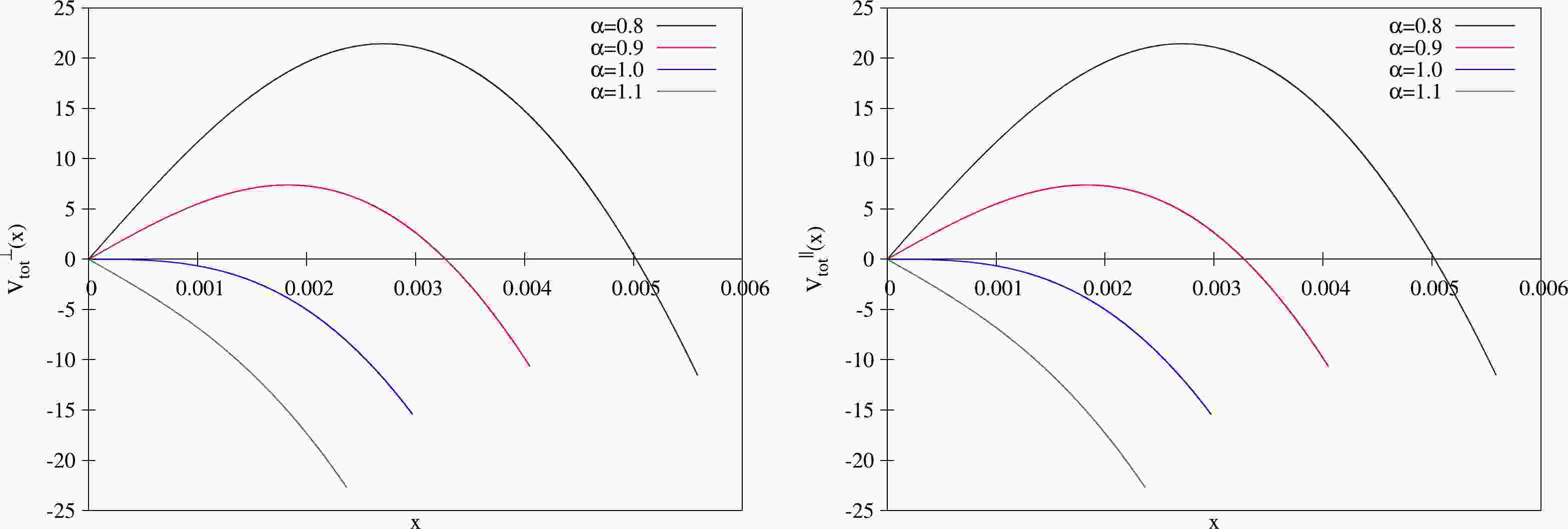
$V_{\rm tot}(x)$ as a function of x for different values of α with fixed$ a=0.2 $ (other cases with different a have a similar picture), where the left panel is for the transverse case, and the right is for the parallel case. As shown in both panels, for$ \alpha<1 $ (or$ E<E_c $ ), the potential barrier is present and the Schwinger effect can occur as a tunneling process. With the increase in E, the potential barrier decreases and finally vanishes at$ \alpha=1 $ (or$ E=E_c $ ). For$ \alpha>1 $ ($ E>E_c $ ), the vacuum becomes catastrophically unstable. These results are in line with those in [10].
Figure 1. (color online)
$V_{\rm tot}(x)$ versus x with$ a=0.2 $ . Left: Transverse case. Right: Parallel case. In both panels from top to bottom,$ \alpha= $ 0.8, 0.9, 1, and 1.1, respectively.To understand how angular momentum modifies the Schwinger effect, we plot
$V_{\rm tot}(x)$ against x for different values of a with fixed$ \alpha=0.9 $ in Fig. 2, where the left panel is for the transverse case, and the right is for the parallel case. In both panels from top to bottom,$ a= $ 0, 0.3, and 0.7, respectively. From these figures, it is clear that as a increases, the height and width of the potential barrier both decrease. As we know, the higher (or the wider) the potential barrier, the harder the produced pairs escape to infinity. Therefore, we can conclude that the inclusion of angular momentum decreases the potential barrier, thus enhancing the Schwinger effect. In other words, the presence of angular momentum enhances the production rate. These results are consistent with previous findings obtained from a soft wall model [25]. Moreover, by comparing the two panels, we find that angular momentum has an important effect in the transverse case compared with the parallel case.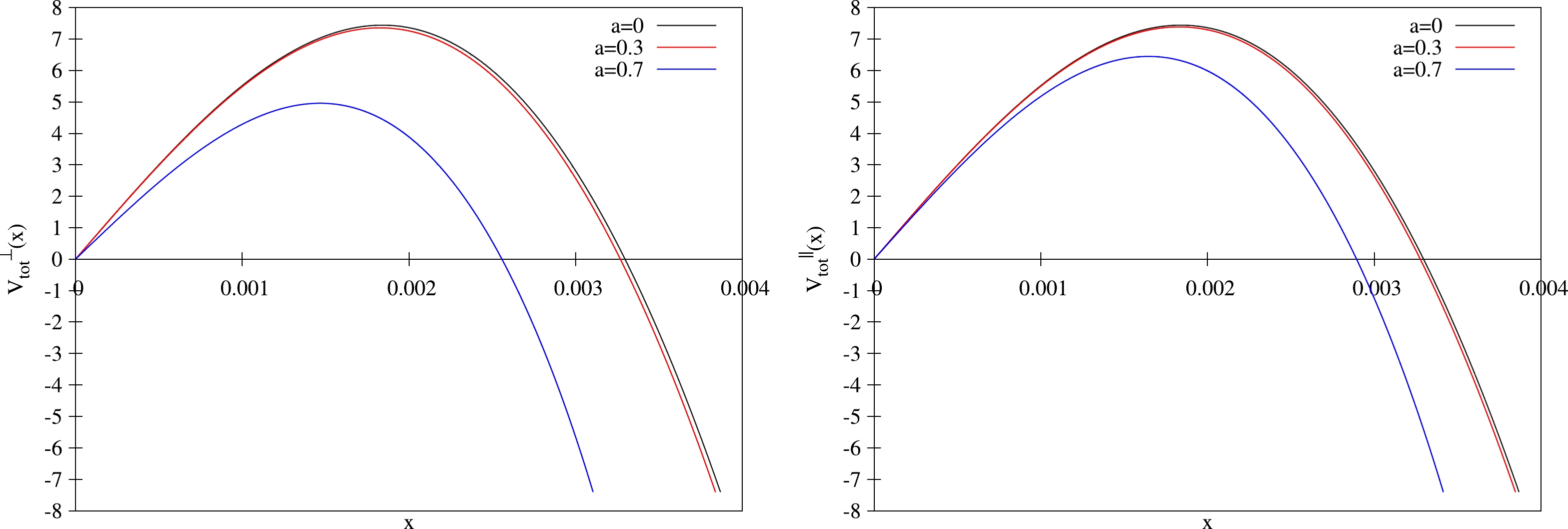
Figure 2. (color online)
$ V_{\rm tot}(x) $ versus x with$ \alpha=0.9 $ for different values of a. Left: Transverse case. Right: Parallel case. In both panels from top to bottom,$ a= $ 0, 0.3, and 0.7, respectively.Furthermore, we can examine how angular momentum affects the critical electric field. To this end, we plot
$ E_c/E_{c0} $ versus a in Fig. 3, where the left panel is for the transverse case, the right is for the parallel case, and$ E_{c0} $ represents the critical electric field at$ a=0 $ . We find that$ E_c/E_{c0} $ decreases as a increases. In particular, when$ a=0.7 $ , the ratio decreased by approximately 8% for the transverse case and 4% for the parallel case. It is known that the smaller the critical electric field, the easier the tunneling process. This is in agreement with the previous potential analysis.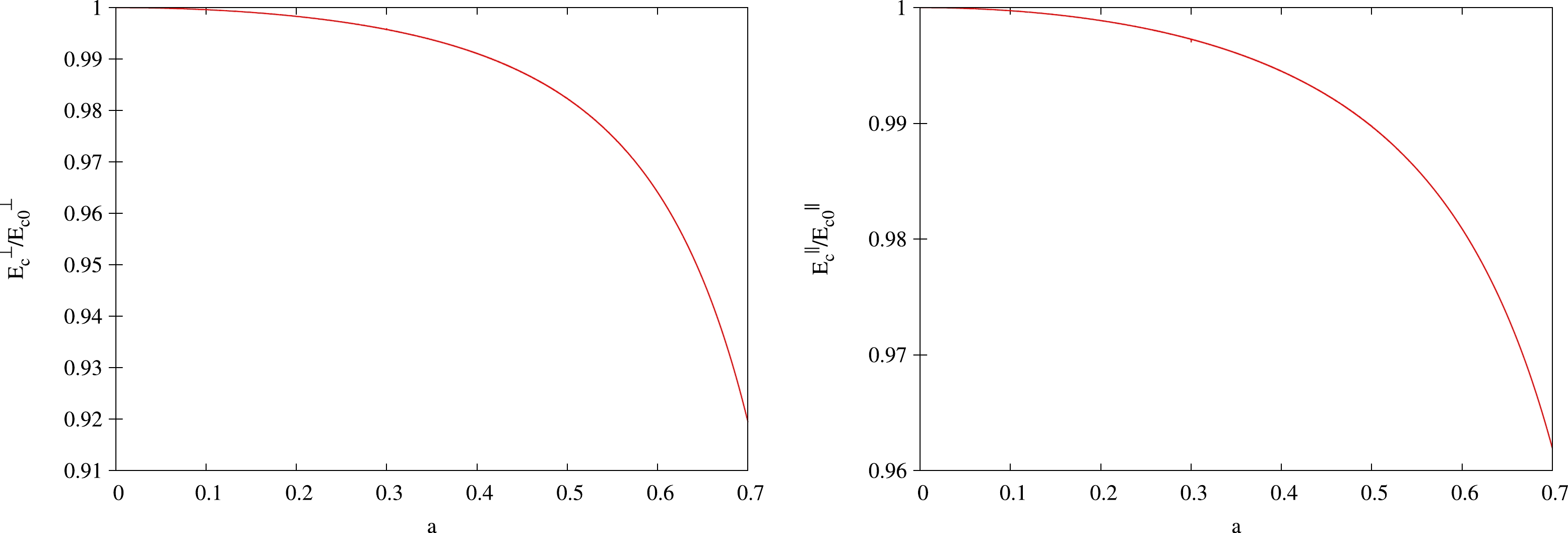
Figure 3. (color online)
$ E_c/E_{c0} $ versus a. Left: Transverse case. Right: Parallel case. -
In this study, we investigate the effect of angular momentum on the holographic Schwinger effect in spinning Myers-Perry black holes. Following the prescription in [10], we calculate the potential between the produced pair by evaluating the classical action of a string attached on a probe D3-brane at an intermediate position in the AdS bulk. It is shown that the inclusion of angular momentum reduces the potential barrier, thus enhancing the Schwinger effect. Therefore, particle pair production would be easier in a rotating medium, in accordance with previous findings obtained from the local Lorentz transformation [25]. Furthermore, the results show that angular momentum has an important effect on the particle pair lying in the transversal plane compared with that along the longitudinal orientation.
Moreover, the results may provide an estimate of how the Schwinger effect changes with
$ \eta/s $ at strong coupling. As shown in (14),$ \eta_\perp/s $ is not affected by a; however,$ \eta_\parallel/s $ decreases as a increases. Here, we do not comment on why only one of the shear viscosities saturates the bound, while the other may violate the bound (a similar situation appeared in several anisotropic backgrounds [61−63]). We then discuss$ \eta_\parallel/s $ . From the above analysis, we find that an increasing a leads to a decreasing$ \eta_\parallel/s $ , and thus the fluid becomes more "perfect". On the other hand, increasing a leads to an enhanced Schwinger effect. Taken together, we may conclude that at strong coupling, as$ \eta/s $ decreases, the Schwinger effect is enhanced.However, there are several problems worthy of further study. First, in this study, we only consider spinning Myers-Perry black holes (
$ a=b $ ). However, what will occur for a general situation ($ a\neq b $ )? Moreover, the potential analysis for the Schwinger effect considered here is essentially within the Coulomb branch associated with the leading exponent corresponding to the on-shell action of the instanton. If possible, the full decay rate may be studied.
Holographic Schwinger effect in spinning black hole backgrounds
- Received Date: 2023-09-04
- Available Online: 2024-01-15
Abstract: We perform a potential analysis for the holographic Schwinger effect in spinning Myers-Perry black holes. We compute the potential between the produced pair by evaluating the classical action of a string attached on a probe D3-brane at an intermediate position in the AdS bulk. We find that increasing the angular momentum reduces the potential barrier, thus enhancing the Schwinger effect, consistent with previous findings obtained via the local Lorentz transformation. In particular, these effects are more visible for the particle pair lying in the transversal plane compared with that along the longitudinal orientation. In addition, we discuss how the Schwinger effect changes with the shear viscosity to entropy density ratio at strong coupling under the influence of angular momentum.


 DownLoad: