


 Abstract
 HTML
HTML Reference
 Related
 PDF
PDF


-
In 2HDM,
$ H^{\pm} $ is allowed to decay freely in fermions and gauge bosons. In Type-I,$ H^{\pm} \longrightarrow AW^{\pm} $ (decay to a neutral Higgs "A" and "W-boson") is a dominant channel. The decay mode into$ \tau^{+}\nu_\tau $ reaches branching ratios of more than 90$ \% $ below the$ t\bar{b} $ threshold, and the muonic one ranges within a few$ 10^{-4} $ [1]. All other leptonic decay channels of the charged Higgs bosons are not important to be considered. There is a fermiophobic charged Higgs decay for large$\tan\beta$ values that follows$ H^{\pm}\rightarrow W^{\pm}\phi $ ($ \phi=h, H, A $ ) if kinematically allowed; it would be the dominant decay even for virtual$ W^{\pm} $ . Thus, it is the most interesting mode of decay for larger$\tan\beta$ values. In Type-I 2HDM, the bosonic decays of light$ H^{\pm} $ were recently studied at the LHC [3]. For decay processes$ H^{\pm}\rightarrow W^{\pm}A $ and$ H^{\pm}\rightarrow W^{\pm}h $ , the branching ratios were calculated in [3]. The decay process$ H^{\pm}\rightarrow W^{\pm}h $ reaches a BR of 10% below the top-bottom threshold at$\tan\beta$ values in the interval 2−3 and$ m_{H^{\pm}} $ = 160 GeV.For production process
$ pp \rightarrow tb H^{\pm} $ , which is generally the dominant mode for$ H^{+} $ , SM inclusive processes with top-quark pairs inevitably constitute an important background regardless of how ϕ decays [4]. Hence, for more conventional 2HDM scenarios, the signal process from$ \phi \rightarrow \tau\tau $ and$ \phi \rightarrow bb $ constitutes a promising research line near the alignment limit [5, 6]. Moreover, in 2HDM, for BR($ \phi \rightarrow \tau\tau $ ) and BR($ \phi \rightarrow bb $ ) with the relative size predicted under additional model assumptions, the search results from the two signatures may be combined to improve the sensitivity coverage of the 2HDM parameter space. Note that${\rm 2HDMC-1.7.0}$ [7] is used to apply theoretical constraints and set experimental bounds. For this purpose, the HiggsBounds [8] and HiggsSignals [9] libraries are interfaced with 2HDMC. In addition, ScannerS [10] is used to establish the most recent experimental bound on selected parameters and determine whether it is allowed experimentally. -
The scalar potential of 2HDM [11] has 14 parameters, including the charge and CP violations. The general term for this scalar potential is
$ \begin{aligned}[b] V=&m^2_{11} \Phi^{\dagger}_1 \Phi_1 + m^2_{22} \Phi^{\dagger}_2 \Phi_2 - m^2_{12} \biggl\{ \Phi^{\dagger}_1 \Phi_2 + h.c. \} + \frac{\lambda_1}{2} (\Phi^{\dagger}_1 \Phi_1)^2 \\&+ \frac{\lambda_2}{2} (\Phi^{\dagger}_2 \Phi_2)^2 + \lambda_3 (\Phi^{\dagger}_1 \Phi_1)(\Phi^{\dagger}_2 \Phi_2) + \lambda_4 (\Phi^{\dagger}_1 \Phi_2) (\Phi^{\dagger}_2 \Phi_1) \\&+ \biggl\{ \frac{\lambda_5}{2} (\Phi^{\dagger}_1 \Phi_2)^2 + \left[ \lambda_6 (\Phi^{\dagger}_1 \Phi_1) + \lambda_7 (\Phi^{\dagger}_2 \Phi_2) \right] (\Phi^{\dagger}_1 \Phi_2) + h.c. \biggl\}, \end{aligned} $

(1) where
$ (\lambda_{i}, i = 1,2,3,...., 7) $ are dimensionless coupling parameters, and$ m^2_{11}, m^2_{22} $ , and$ m^2_{12} $ are squares of masses. To treat the 2HDM potential as charge and parity conserving potential, all the parameters should be real. The vacuum expectation value VEV is obtained by each scalar-doublet when the electroweak symmetry breaks. The two doublets are$ <\Phi_1>=\left(\begin{array}{*{20}{c}}{0}\\{\dfrac{V_1}{\sqrt{2}}}\end{array} \right),\quad <\Phi_2>=\left(\begin{array}{*{20}{c}}{0}\\{\dfrac{V_2}{\sqrt{2}}} \end{array}\right). $

(2) These two doublets lead to eight fields, among which three correspond to massive
$ W^{\pm} $ and$ Z^0 $ vector bosons, and the remaining five fields lead to five physical Higgs bosons:$ \Phi_i=\left(\begin{array}{*{20}{c}}{\Phi^+_i}\\{\dfrac{(V_i+\rho_i+\iota\eta_i)}{\sqrt{2}}}\end{array}\right), $

(3) where i = 1, 2 with
$V_1=V\cos\beta,~ V_2=V\sin\beta~ {\rm and}~ V_1,V_2 \geq 0$ . The condition$V_{\rm SM} = \sqrt{V^2_1+V^2_2}$ is satisfied. The experimentally obtained value of$ V_{SM} $ is 246.22 GeV. The obtained fields are expressed as$ \begin{aligned}[b] &\binom{\rho_a}{\rho_b}= \begin{pmatrix} \cos\alpha & -\sin\alpha\\ \sin\alpha & \cos\alpha \end{pmatrix} \binom{H}{h} , \\& \binom{\eta_a}{\eta_b} = \begin{pmatrix} \cos\beta & -\sin\beta\\ \sin\beta & \cos\beta \end{pmatrix} \binom{G^0}{A} \end{aligned} $

(4) and
$ \left(\begin{array}{*{20}{c}} {\Phi^{\dagger}_a}\\{\Phi^{\dagger}_b}\end{array}\right)= \begin{pmatrix} \cos\beta & -\sin\beta\\ \sin\beta & \cos\beta \end{pmatrix} \left(\begin{array}{*{20}{c}}{G^{\dagger}}\\{H^{\dagger}}\end{array}\right). $

(5) The mass-matrix of charged Higgs states is diagonalized by a rotational angle defined as
$\tan\beta = \dfrac{V_{2}}{V_{1}}$ . Similarly, the mass-matrix of scalar Higgs states is diagonalized by a rotational angle α that satisfies the relation$ \tan(2\alpha)=\frac{2(-m^2_{12}+\lambda_{345}V_1V_2)}{m^2_{12}(V_2/V_1 - V_1/V_2)+\lambda_1V^2_1-\lambda_2V^2_2} $

(6) where
$ \lambda_{345}=\lambda_3+\lambda_4+\lambda_5 $ . -
The general potential of 2HDM is complex compared to the one in the standard model SM. In particular, 2HDM imposes theoretical constraints on the potential to guarantee the stability of the potential.
The Higgs potential should be positive throughout the field space. This ensures that a stable vacuum configuration for asymptotically large field values is maintained. The quartic terms are the leading terms at large field space values. In this context, the following substitutions are helpful:
$\mid \Phi_1 \mid=r \cos \phi , \quad \mid\Phi_2\mid=r\sin\phi \quad {\rm and} \quad \frac{\Phi_1\Phi^{\dagger}_2}{\mid\Phi_1\mid\mid\Phi_2\mid} =\rho\exp(\iota\theta), $

(7) where
$\rho=\mid0-1\mid , \quad \theta=\mid0-2\pi\mid \quad {\rm and} \quad \phi=\mid0-\dfrac{\pi}{2}\mid$ . After making these substitutions and omitting the common factor$ r^4 $ , the quartic terms of the potential can be expressed as$ \begin{aligned}[b] V_{(4)}=&\frac{1}{2}\lambda_1 \cos^4\phi + \frac{1}{2}\lambda_2 \sin^4\phi + \lambda_3\cos^2\phi \sin^2\phi\\&+\lambda_4\rho^2\cos^2\phi \sin^2\phi + \lambda_5\rho^2 \cos^2\phi \sin^2\phi \cos2\theta \\&+ [\lambda_6 \cos^2\phi + \lambda_7 \sin^2\phi]2\rho \cos\phi \sin\phi \cos\theta. \end{aligned} $

(8) From the above equation, we can see that the potential will be positive if
$ \begin{aligned}[b]& \lambda_1>0 , \quad \lambda_2>0 , \quad \lambda_3>-\sqrt{\lambda_1\lambda_2}\; , \\& \lambda_3 + \lambda_4 - |\lambda_5| > -\sqrt{\lambda_1\lambda_2} \end{aligned} $

(9) If
$ \lambda_{6} = 0 = \lambda_{7} $ , there are necessary and sufficient conditions to ensure the positivity of the quartic potential.If either
$ \lambda_{6} \not= 0 $ or$ \lambda_{7} \not= 0 $ for the case they are real, one finds that$ 2 |\lambda_6+\lambda_7| ~ < ~ \frac{\lambda_1 + \lambda_2}{2}+\lambda_3+\lambda_4+\lambda_5 . $

(10) Scattering matrices are unitary in order to conserve probability. In the theory of weak couplings, the contribution of higher order terms decreases gradually. By contrast, in the theory of strong couplings, individual contributions increase arbitrarily. The eigenvalues (
$ L_i $ ) of S-matrices must satisfy the condition$ L_i \leq 16\pi $ in order to achieve the tree-level unitarity that means the saturation of S-matrices up to tree-level unitarity.Perturbation constraints require that the quartic Higgs couplings must satisfy the condition
$ \mid C_{H_{i},H_{j},H_{k},H_{l}} \mid \leq 4\pi $ . One can imagine that some interaction channels are non-perturbative while others are perturbative. Note that setting$ \mid \lambda_i \mid = 4\pi\xi $ is an alternative approach to explain this constraint, where$ \xi = 0.8 $ 1 . This sets$ \mid \lambda_i \mid \leq 10 $ for$ \lambda_i $ as the upper bound.Alongside theoretical constraints, there are also experimental constraints coming from B-Physics and various experiments on different colliders from recent Higgs searches. Here we discuss some important constraints. Moreover, using SuperIso V.3.2 [12], we list the SM prediction values provided in this category. The Standard Model BR for
$(B_\mu \rightarrow \tau\nu)_{\rm SM}$ reported in [12] is$ {\rm BR} (B_\mu\rightarrow \tau\nu)_{\rm SM} = (1.01 \pm 0.29) \times 10^{-4} . $

(11) The standard model estimation may, in fact, be contrasted with the most recent heavy flavour averaging (HFAG) result [13]:
$ {\rm BR} (B_\mu\rightarrow \tau\nu)_{\rm exp} = (1.64 \pm 0.34) \times 10^{-4}, $

(12) and the ratio becomes
$ R^{\rm exp}_{\rm SM} = \frac{{\rm BR}(B_\mu\rightarrow \tau\nu)_{\rm exp}}{{\rm BR}(B_\mu\rightarrow \tau\nu)_{\rm SM}} = 1.62 \pm 0.54 . $

(13) This causes the exclusion of two sectors of
$(\tan\beta)/m_{H^\pm}$ ratio in 2HDM [14]. This implies that for$\tan\beta \geq 1$ , the mass of charged Higgs must be greater than 800 GeV for Type-II 2HDM[15]. Given that the ($ B_\mu \rightarrow {\tau}{\nu}_{\tau} $ ) decay depends on$ \mid V_{ub} \mid $ , the ($ B_\mu \rightarrow Dl \nu $ ) (semi-leptonic) decay also depends on$ \mid V_{ub} \mid $ , which is more precisely known than$ \mid V_{ub} \mid $ . Moreover, the branching ratio of ($ B_\mu \rightarrow {\tau}{\nu}_{\tau} $ ) is fifty times greater than the branching ratio of ($ B_\mu \rightarrow {\tau}{\nu} $ ) in the standard model, but it is still difficult to detect because two neutrinos exist in its final state. The 2HDM deals only with the numerator of the ratio$ {\xi}_{Dl\nu_\tau} = \frac{{\rm BR}(B\rightarrow D{\tau}{\nu}_{\tau})}{{\rm BR}(B\rightarrow Dl{\nu}_{\tau})} $

(14) and allows reducing theoretical uncertainties to some extent. The experimental outcomes by BaBar collaborations and SM predictions [14] are
$ {\xi}^{\rm SM}_{Dl{\nu}_{\tau}} = (29.7 \pm 3) \times 10^{-2} ,$

(15) $ {\xi}^{\rm exp}_{Dl{\nu}_{\tau}} = (44.0 \pm 5.8 \pm 4.2) \times 10^{-2} . $

(16) For (
$ B \rightarrow X_s\gamma $ ), this special transition is mediated by$ H^{\pm} $ and includes Flavor-changing neutral current (FCNC) and$ W^{\pm} $ contributions. Regarding the respective BR, the contribution of charged Higgs is always positive when it comes to probing Type-II 2HDM; this can be used efficiently. For this transition, the NNLO-SM predicted$(3.34\pm0.22)\times 10^{-4}$ for${\rm BR} (B \rightarrow X_s\gamma)_{\rm SM}$ [16]. Therefore, for${\rm BR} (B \rightarrow X_s\gamma)_{\rm exp}$ , the recently experimentally calculated value is$ (3.32\pm0.15)\times 10^{-4} $ . For Type-II Yukawa interactions, this constraint excludes the light-charged Higgs. Higher order analysis [17] estimated a lower limit of 380 GeV at 95% C.L. for$ M_{H^{\pm}} $ . However, it is important to mention that the bound in [17] does not include novel experimental and theoretical predictions and hence the numerical results may be outdated.For (
$ D_S \rightarrow \tau\nu $ ), the SM prediction is$ (3.32\pm0.15)\times 10^{-4} $ [12] for$f_{Ds} = 0.248 \pm 2.5~{\rm GeV}$ [18] and the updated experimental calculation for${\rm BR}(D_s \rightarrow \tau\nu)_{\rm exp}$ is$ (5.51\pm 0.24)\times10^{-2} $ [19] for ($ B_{d/s} \rightarrow \mu^+\mu^- $ ). At large$\tan \beta$ values, the lower limit on charged Higgs mass$ m_{H^{\pm}} $ is given in [20]. For decays${\rm BR}(B_s \rightarrow {\mu}^+{\mu}^+)_{\rm SM}$ and${\rm BR} (B_d \rightarrow {\mu}^+{\mu}^+)_{\rm SM}$ , SM predictions are$ (3.54\pm0.27)\times10^{-9} $ and$(1.1\pm0.1)\times 10^{-9}$ , respectively [12]. Experimental results for the limits of these decays at 95% C.L. are${\rm BR} (B_s \rightarrow {\mu}^+{\mu}^+)_{\rm exp} < 4.5 \times 10^{-9}$ and${\rm BR} (B_d \rightarrow {\mu}^+{\mu}^+)_{\rm exp} < 1.0 \times 10^{-9}$ reported by the LHCb collaboration [21]. If the results from ATLAS and CMS [22] concerning the aforementioned limits are also added, then stricter limits are${\rm BR} (B_s \rightarrow {\mu}^+{\mu}^+)_{\rm exp} < 4.2 \times 10^{-9}$ and${\rm BR}(B_d \rightarrow {\mu}^+{\mu}^+)_{\rm exp} < 8.1 \times 10^{-10}$ . -
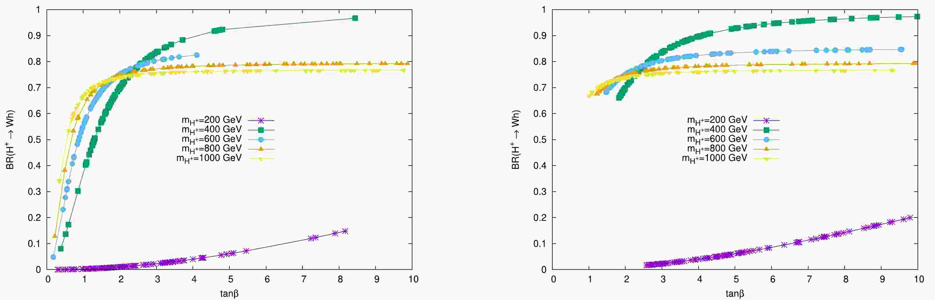
The branching ratios were calculated using HDECAY [23] through the anyHdecay interface reported in Ref. [10]. Predictions for gluon-fusion and bb-associated Higgs production at hadron colliders were obtained using tabulated results from SUSHI [24]. The V H-associated (sub)channel cross section predictions were made using the HiggsBounds parametrizations, and the charged Higgs production in association with a top-quark was tested using the HiggsBounds and HiggsSignals. These constraints and calculations were implemented in ScannerS. Figure 1 shows BR
$(H^{+}\rightarrow W^{+}h) $ with respect to$ \tan \beta $ values for different masses of$ m_{H^+} $ . Note that for$ m_{H^{+}}=800 $ and$ 1000 $ GeV, BR$(H^{+}\rightarrow W^{+}h) $ remains between$ 70\% \to 80\% $ . For$ m_{H^+}=600 \, \rm{GeV} $ , the maximum BR exceeds$ 80 \% $ for large$ \tan \beta $ values. For$ \tan \beta > 3 $ , the maximum BR is achieved for$ m_H^+ = 400 $ GeV. For$ m_{H^+}=200 ~\rm{GeV} $ , the BR remains less than$ 20\% $ across the$ \tan \beta $ range.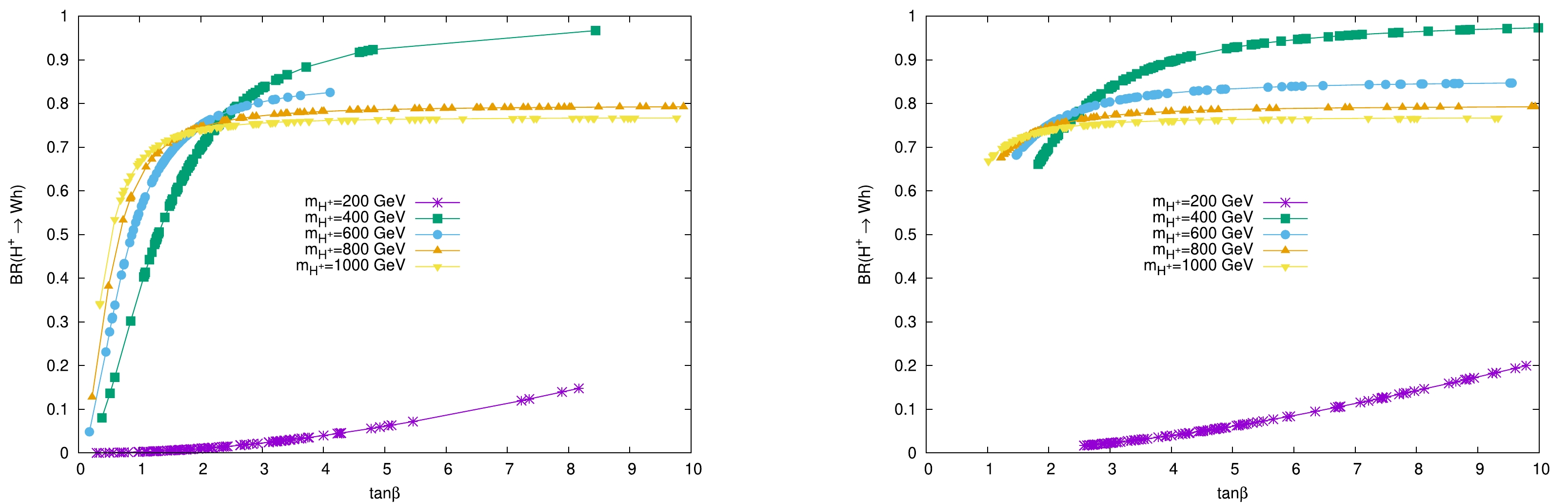
Figure 1. (color online) In Type-I 2HDM,
$\tan\beta$ vs BR($ H^{+}\rightarrow W^{+}h $ ) is scanned in the presence of theoretical (left) and experimental (right) restrictions (constraints) with$ m_{h} $ =125 GeV,$ m_{H} $ =300 GeV,$ m_{H^{+}} $ =$ m_{A} $ =200−1000 GeV, and$\sin(\beta-\alpha)=$ 0.85; we set${m^{2}}_{12}= $ $ \frac{[{m^2}_{H^+}][\tan{\beta}]}{[1+{\tan{\beta}}^2]}$ .Figure 2 shows that, for
$ m_{H^{+}}=200 $ GeV at$2\leq \tan\beta \leq 3$ , BR$(H^{+}\rightarrow tb) $ is dominant, i.e., BR$(H^{+}\rightarrow tb) \approx 100\%$ . Note also from Figs. 1 and 2 that for smaller$\tan \beta$ values, the$ H^+ \to tb $ decay mode is dominant while for higher values,$ H^+ \to Wh $ becomes most probable. However, for$ m_{H^+} = 200 $ GeV, the scenario is different: BR$(H^{+}\rightarrow tb) $ is dominant while BR$(H^{+}\rightarrow Wh) $ is less probable.
Figure 2. (color online) In Type-I 2HDM,
$\tan\beta$ vs BR($ H^{+}\rightarrow $ tb) is scanned in the presence of theoretical (left) and experimental (right) restrictions (constraints) with$ m_{h} $ =125 GeV,$ m_{H} $ =300 GeV,$ m_{H^{+}} $ =$ m_{A} $ =[200−1000] GeV, and$\sin(\beta-\alpha)$ =0.85; we set$ {m^{2}}_{12} $ =$\frac{[{m^2}_{H^+}][\tan{\beta}]}{[1+{\tan{\beta}}^2]}$ .Figure 3 (left) shows the selection of points in the (
$\tan\beta$ ,BR($ H^{+}\rightarrow W^{+}h) $ parameter space when both theoretical and experimental constraints are applied at different charged Higgs masses while Fig. 3 (right) shows the BR($ H^{+}\rightarrow tb $ ) parameter space. The effects of varying the parameters fixed here will be shown and discussed later.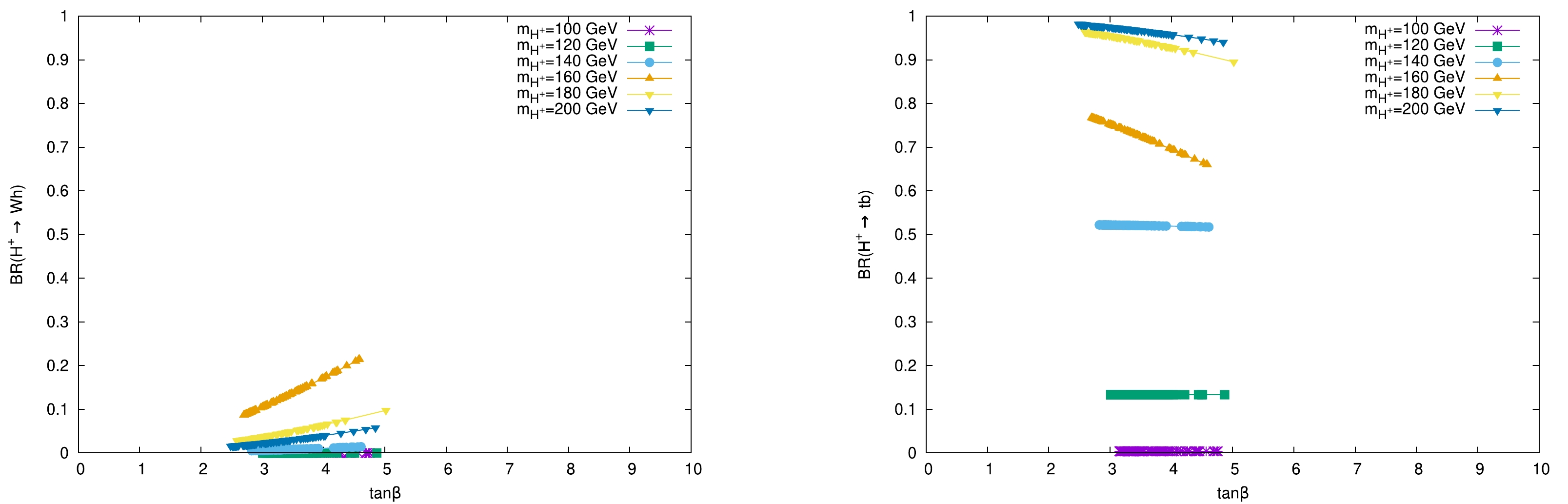
Figure 3. (color online) In Type-I 2HDM, tanβ vs BR(
$ H^{+}\rightarrow W^{+}h $ ) (left)$\tan\beta$ vs BR($ H^{+}\rightarrow t\bar{b} $ ) (right) are scanned in the presence of theoretical and experimental constraints with$ m_{h} $ = 125 GeV,$ m_{H} $ =300 GeV,$ m_{H^{+}} $ =$ m_{A} $ =[100−200] GeV, and$\sin(\beta-\alpha)$ = 0.85; we set${m^{2}}_{12}=\frac{[{m^2}_{H^+}][\tan{\beta}]}{[1+{\tan{\beta}}^2]}$ .Figure 4 shows that for
$\tan{\beta} \in [2,~ 3]$ and$m_{H^+} \in $ [150, 210], BR$(H^{+} \rightarrow W^{+}h) $ emerges in the region from [0.06, 0.07], represented in the vertical palette. Note also that for$\tan{\beta} \in [2,~ 3]$ and$m_{H^+} \in [150,~ 210]$ , BR$(H^{+} \rightarrow tb) $ emerges in the region from [0.65, 0.7], represented in the vertical palette. For the same range of$ m_{H^{+}} $ and$\tan\beta$ , BR$(H^{+}\rightarrow tb) $ becomes boosted towards the point that it overrides all the other decay modes. Note that, when going over light-charged Higgs to heavy-charged Higgs, there are most observable states that exist in the defined region.
Figure 4. (color online) In Type-I 2HDM,
$ m_{H^{+}} $ against$\tan\beta$ BR($ H^{+}\rightarrow W^{+}h $ ) (left) and BR($ H^{+}\rightarrow t\bar{b} $ ) (right) is scanned in the presence of theoretical and experimental constraints with$ m_{h} $ =125 GeV,$ m_{H} $ =300 GeV,$ m_{H^{+}} $ =$ m_{A} $ , and$\sin(\beta-\alpha)$ =0.85; we set$ {m^{2}}_{12} $ =$\frac{[{m^2}_{H^+}][\tan{\beta}]}{[1+{\tan{\beta}}^2]}$ . At a 95% confidence-level (CL), yellow colour zones are omitted from LHC Higgs data, and black/grey zones are omitted from theoretical restrictions (constraints).Note from Fig. 5 and Fig. 6 that the experimental bounds do not pose any further constraints for
$ H^{+}\rightarrow W^{+}A $ and$ H^{+}\rightarrow tb $ .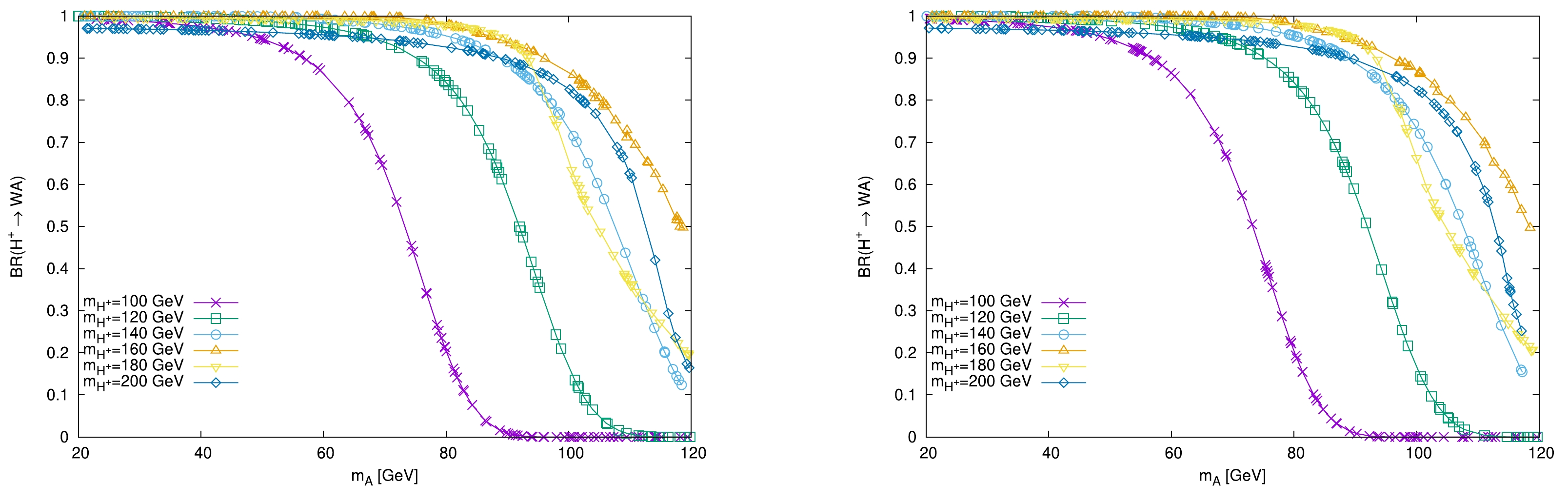
Figure 5. (color online) In Type-I 2HDM,
$ m_A $ vs BR($ H^{+}\rightarrow W^{+}A $ ) is scanned in the presence of theoretical (left) and experimental (right) restrictions (constraints) with$ m_{h} $ =125 GeV,$ m_{H} $ =300 GeV,$ m_{H^{+}} $ =[100−200] GeV,$\tan\beta$ =5,$\sin(\beta-\alpha)=0.85$ , and$ {m^{2}}_{12} $ =16000$ {\rm GeV}^{2} $ .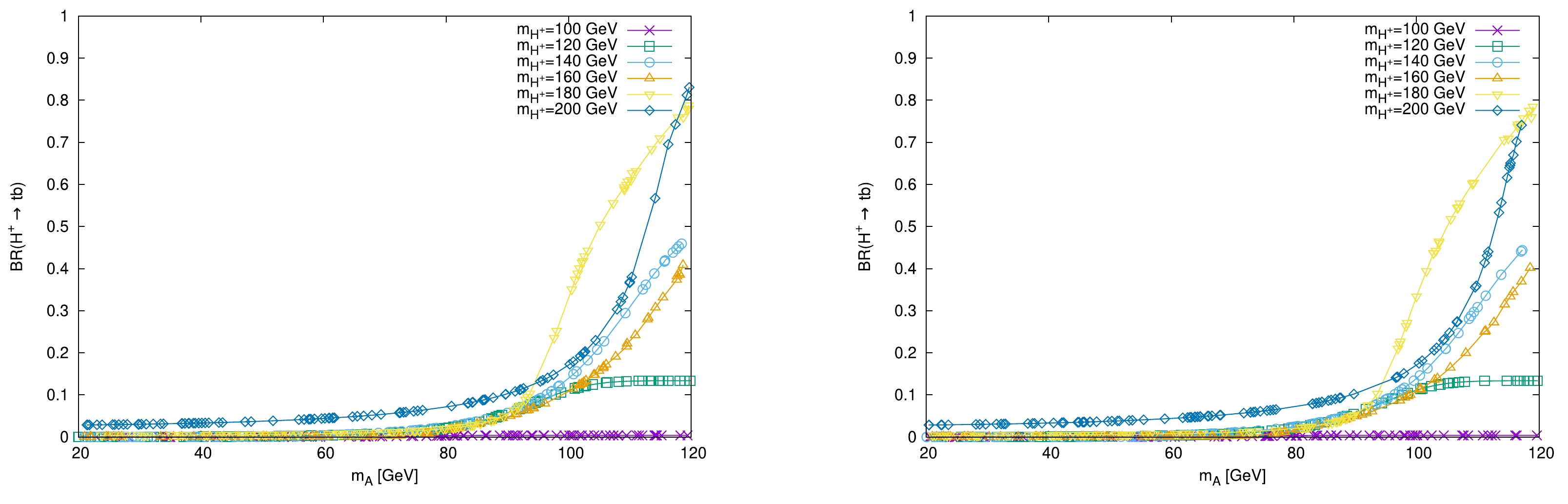
Figure 6. (color online) In Type-I 2HDM,
$ m_A $ vs BR($ H^{+}\rightarrow $ tb) is scanned in the presence of theoretical (left) and experimental (right) restrictions (constraints) with$ m_{h} $ =125 GeV,$ m_{H} $ =300 GeV,$ m_{H^{+}} $ = [100−200] GeV,$\tan\beta$ =5,$\sin(\beta-\alpha)=0.85$ , and$ {m^{2}}_{12} $ =16000 GeV$ ^{2} $ .Figure 7 shows that, except for some short regions, BR
$(H^{+}\rightarrow WA) $ is dominant and becomes 100% in the mass range$m_{H^+} = [100,~ 200]$ . The tb-decay mode is the least dominant because of the kinematic constraints; it only becomes prominent for$ m_{H^+} $ above 180 GeV. It is clear that BR$(H^{+}\rightarrow WA) $ could be the leading decay channel for$ m_{A} \leq 100 $ GeV and any mass of$ m_{H^+} $ .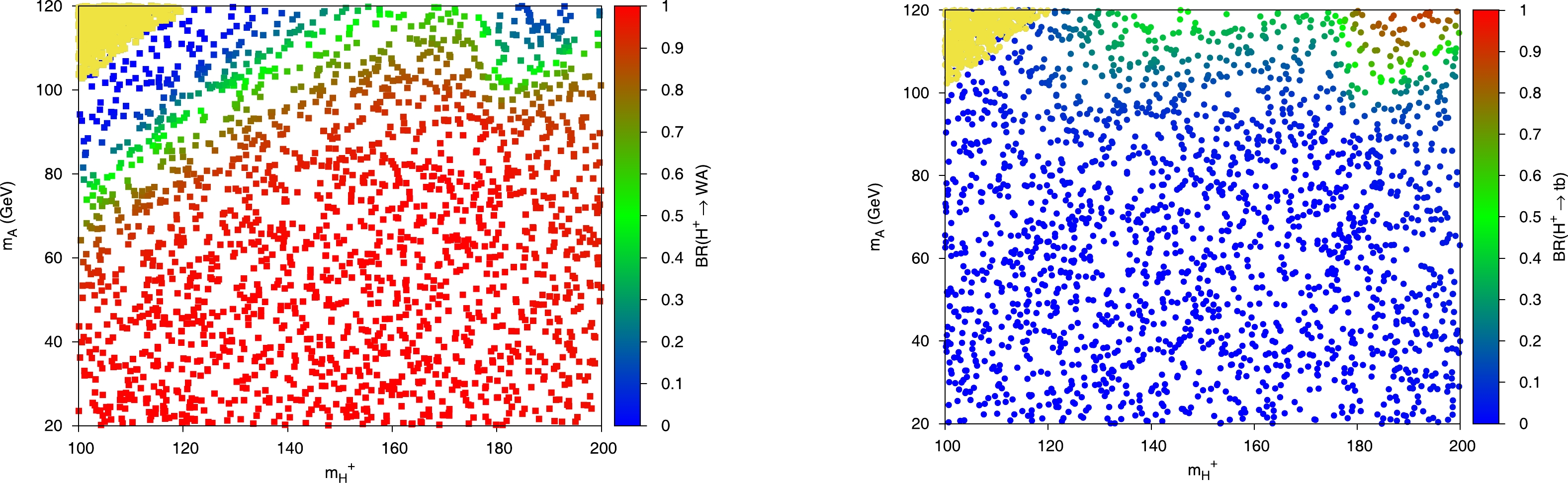
Figure 7. (color online) In Type-I 2HDM,
$ m_{H^{+}} $ vs$ m_{A} $ BR($ H^{+}\rightarrow WA $ ) (left) and BR($ H^{+}\rightarrow $ tb) (right) is scanned in the presence of theoretical and experimental restrictions (constraints) with$ m_{h} $ = 125 GeV,$ m_{H} $ = 300 GeV,$\tan\beta$ =5,$\sin(\beta-\alpha)=1$ , and$ {m^{2}}_{12} $ = 16000$ {\rm GeV}^{2} $ . At a 95% confidence level (CL), the yellow zone is omitted from the LHC Higgs data.Figure 8 shows a scan over a value of
$ m_{H^{+}} $ arbitrarily chosen and fixed between 160 GeV and 180 GeV, i.e., 170 GeV. It shows the size of BR($ H^{\pm}\rightarrow W^{\pm{*}}h + W^{\pm{*}}A $ ) over$\sin(\beta-\alpha)$ vs$\tan\beta$ (left) and$ {m^{2}}_{12} $ vs$\tan\beta$ (right). The right panel shows the effect of the soft$ Z_2 $ breaking term$ m_{12} $ . It is clear that for some special choices of$\tan\beta$ and$ {m^{2}}_{12} $ , BR($ H^{\pm}\rightarrow W^{\pm{*}}h + W^{\pm{*}}A $ ) could reach a value above 50% for$\sin(\beta - \alpha)$ between 0.6 and 0.7. The right panel is represented by fixing$\sin(\beta - \alpha)$ at 0.65; the variation is shown as a function of$ m_{12}^2 $ . The favorable green zones are located in regions with$ m_{12}^2 > 12,000 $ GeV.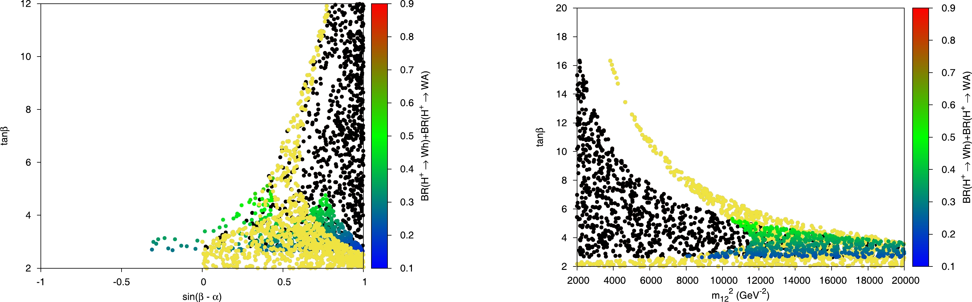
Figure 8. (color online) In THDM Type-I, BR(
$ H^{+}\rightarrow W^{+}h $ )+BR($ H^{+}\rightarrow W^{+}A $ ) is mapped over$ \sin(\beta-\alpha $ ) vs$ \tan\beta $ with$ {m^{2}}_{12} $ = 5000$ {\rm GeV}^{2} $ on the left while$ {m^{2}}_{12} $ vs$ \tan\beta $ with$ \sin(\beta-\alpha) $ = 0.65 is shown on the right. Other parameters are$ m_{h} $ =$ m_{A} $ = 125 GeV,$ m_{H} $ = 300 GeV, and$ m_{H^{+}} $ = 170 GeV. At a 95% confidence-level (CL), yellow colour zones are omitted from the LHC Higgs data, and black/grey zones are omitted from theoretical restrictions (constraints).Figure 9 shows
$ \sigma \times $ BR($ t\rightarrow H^{+}b $ )$ \times $ BR($ H^{+}\rightarrow W\phi $ ) with$ \phi=h $ (left) and$ \phi=A $ (right) over the light charged Higgs mass range 120−180 GeV in proton-proton collisions at three distinct center-of-mass energies,$ \sqrt{s} $ = 8 TeV,$ \sqrt{s} $ = 13 TeV, and$ \sqrt{s} $ = 14 TeV, represented with three different distinguishable colors.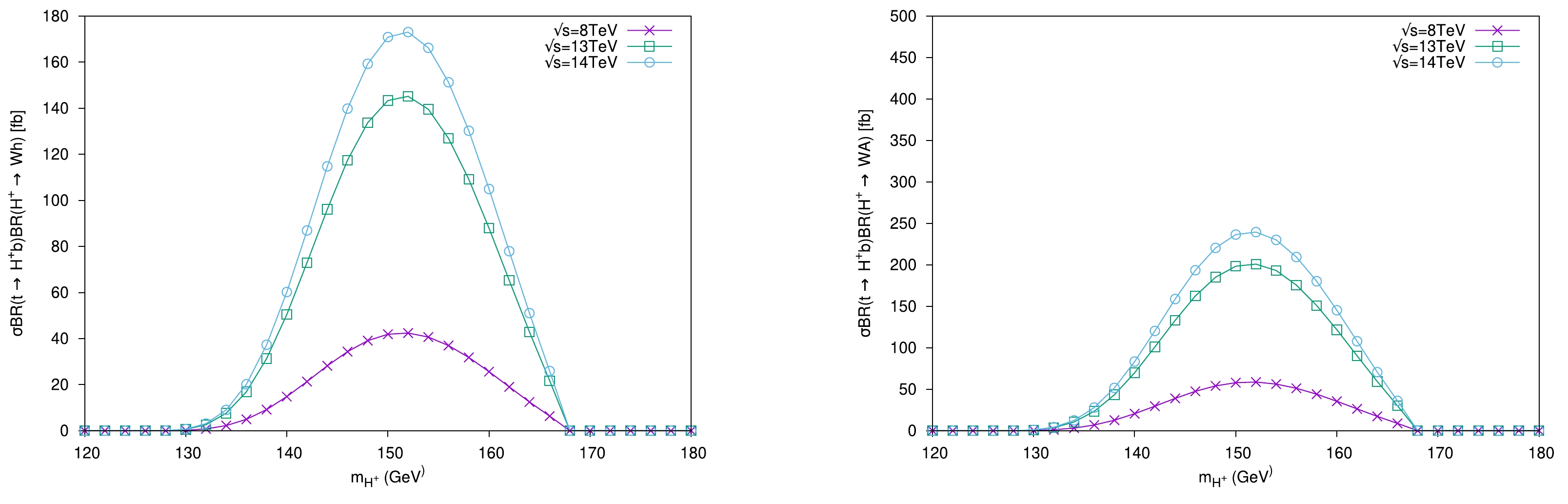
Figure 9. (color online) In Type-I 2HDM, the rates for
$ \sigma(pp\rightarrow t\bar{t}) \times {\rm BR}(t\rightarrow H^{+}b) \times {\rm BR}(H^{+}\rightarrow W\phi) $ with$ \phi=h $ (left) and$ \phi=A $ (right) are scanned as a function of$ m_{H^{+}} $ at$ \sqrt{s} $ = 8 TeV,$ \sqrt{s} $ = 13 TeV, and$ \sqrt{s} $ = 14 TeV with$ m_{h} $ = 125 GeV,$ m_{H} $ = 300 GeV,$ m_{A} $ = 125 GeV,$\tan\beta$ = 5,$\sin(\beta-\alpha)$ = 0.85, and$ {m^{2}}_{12} $ = 16000$ {\rm GeV}^{2} $ .Figure 10 shows the variation of
$ \sigma \times $ BR($ t\rightarrow H^{+}b $ )$ \times $ BR($ H^{+}\rightarrow W\phi $ ) as a function of$\tan \beta$ , ranging between 2−20, while keeping the charged higgs mass$ m_H^{\pm} $ fixed at 170 GeV. Three distinct curves represent different center of mass energies, as described earlier.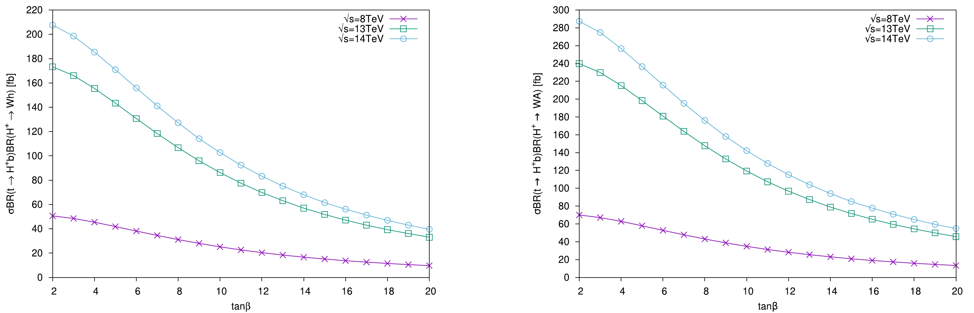
Figure 10. (color online) In Type-I 2HDM, the rates for
$\sigma(pp\rightarrow t\bar{t}) \times {\rm BR}(t\rightarrow H^{+}b) \times {\rm BR}(H^{+}\rightarrow W\phi)$ with$ \phi=h $ (left) and$ \phi=A $ (right) are scanned as a function of$\tan\beta$ at$ \sqrt{s} $ = 8 TeV,$ \sqrt{s} $ = 13 TeV and$ \sqrt{s} $ = 14 TeV with$ m_{h} $ = 125 GeV,$ m_{H} $ = 300 GeV,$ m_{H^{+}} $ = 150 GeV,$ m_{A} $ = 125 GeV,$ \sin(\beta-\alpha) $ = 0.85, and$ {m^{2}}_{12} $ = 16000$ {\rm GeV}^{2} $ . -
Multivariate Analysis (MVA) [25] methods have been widely used in many studies conducted in ATLAS and CMS to discriminate signals over backgrounds in searches that include complex multi-particle final states, e.g., the current analysis of
$pp \rightarrow H^{+} t \rightarrow t\bar{t}b \rightarrow 3bjets + 4 jets$ . Based on machine learning, the multivariate classification technique is fundamental for many data analysis methods. It is included in the ROOT framework; the TMVA toolkit encompasses a large diversity of classification algorithms. Training, testing, progress assessment, and use of all accessible classifiers are executed simultaneously and are simple to use. Supervised Machine Learning is used in all TMVA methods, which exploit training events to determine the required outputs. When implementing a machine learning algorithm for an analysis, a training process is required in which the algorithm observes already known events (i.e., simulated samples where right or wrong is predefined) and learns the difference between background and signal events.We selected three different techniques for charged Higgs production in association with top quark: Boosted Decision Trees (BDT), maximum Likelihood (LH) method, and Multilayer Perceptron (MLP). The production samples are based on Monte Carlo (MC) simulations of the signal and most backgrounds at
$ \sqrt{s} = 100 $ TeV. The main background consists of production of single top quarks in association with W boson, single top production in s-channel process, and top anti-top quark pair production. The charged Higgs mass was set at 800 GeV, while the signal contained a physical single charged Higgs boson associated with top quark. Both signal and background processes were produced with Pythia 8 embedded in MadGraph [26] and the detector simulation was performed by Delphes [27]. Both the signal and background samples were analyzed with the Toolkit for MultiVariate Analysis (TMVA) available in ROOT, which includes a large variety of multivariate classification algorithms. Events were selected according to the presence of a required number of objects in the final state. In signal events including at least 7 jets, there must be at least three b-jets and 4 light jets. In addition, a missing transverse energy larger than 30 GeV, a transverse momentum greater than 20 GeV, and an absolute pseudo rapidity less than 3.0 were applied as selection cuts for background suppression and signal enhancement.The responses of the three classifiers are shown in Fig. 11, and their values for Area Under the Curve (AUC) are extracted in the form of Table 1. These results are satisfactory except for the Likelihood method.
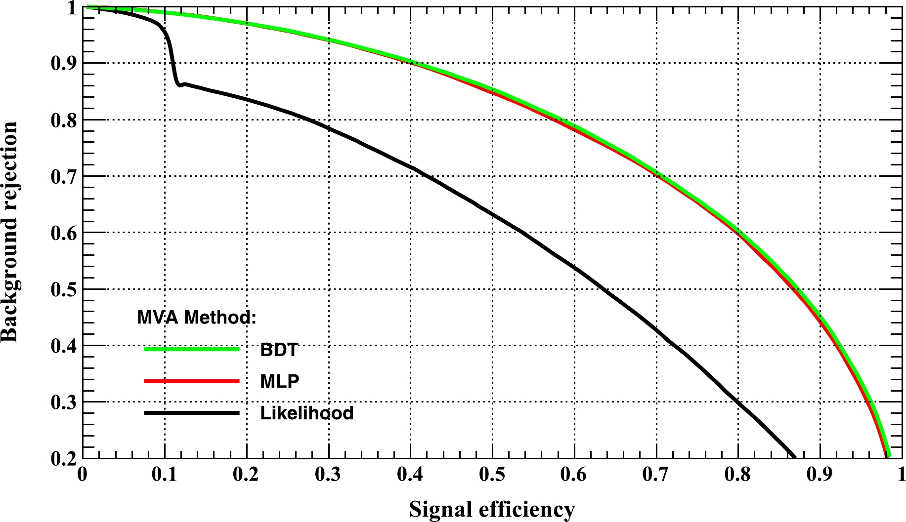
Figure 11. (color online) The y-axis represents the background rejection, i.e., how much background is lost after a given cut on the BDT, MLP, and Likelihood outputs, while the x-axis represents how much signal is kept. This gives an idea on how a set of chosen variables is discriminated.
MVA Classifier AUC(with cuts) MLP 0.777 BDT 0.781 Likelihood 0.582 Table 1. MVA Classifier Area Under the Curve (AUC) with cuts; the values are satisfactory, except for the Likelihood method.
We also calculated the statistical significance (SS) from signal (S) and background (B) events, where significance is defined as
$ SS= S /\sqrt{S+B} $ . The results are presented in Table 2. This enables the observability of the charged Higgs at FCC designed integrated luminosity.MVA Classifier Optimal-Cut $\dfrac{S}{\sqrt{S+B}}$ 

Sig-Eff Bkg-Eff MLP 0.2046 105.575 0.924 0.6079 Likelihood −3.9495 100.004 1 0.9998 BDT −0.0944 105.89 0.9306 0.6141 Table 2. Optimal-Cuts, Signal-Background ratio, signal, and Background efficiency for a number of signals and backgrounds under the application of cuts.
For a given number of signal and background events, Fig. 12 depicts the significance
$ S/\sqrt{S + B} $ as a function of the BDT cut value in (a) and Likelihood cut in (b). This is the parameter that most properly indicates the training performance. The significance output is used to evaluate the corresponding method performance: a higher significance indicates a better classifier. However, statistics must be considered, which means that the signal efficiency that corresponds to the ideal cut value must be considered. A lot of signal are filtered out if this number is really low. If the real data exhibit low statistics, the quality of the cut cannot be guaranteed because the output distribution differs from that of the training sample. Figure 13 shows the MLP cut efficiencies as a function of the applied cut value. MLP and BDT present similar values of significance. These values are higher than that of the Likelihood method.
Figure 12. (color online) Signal efficiency, background efficiency, signal purity, signal efficiency multiplied by purity, and significance
$ S/\sqrt{S+B} $ as a function of the BDT cut level in (a) and Likelihood output level in (b) as a function of the BDT cut value.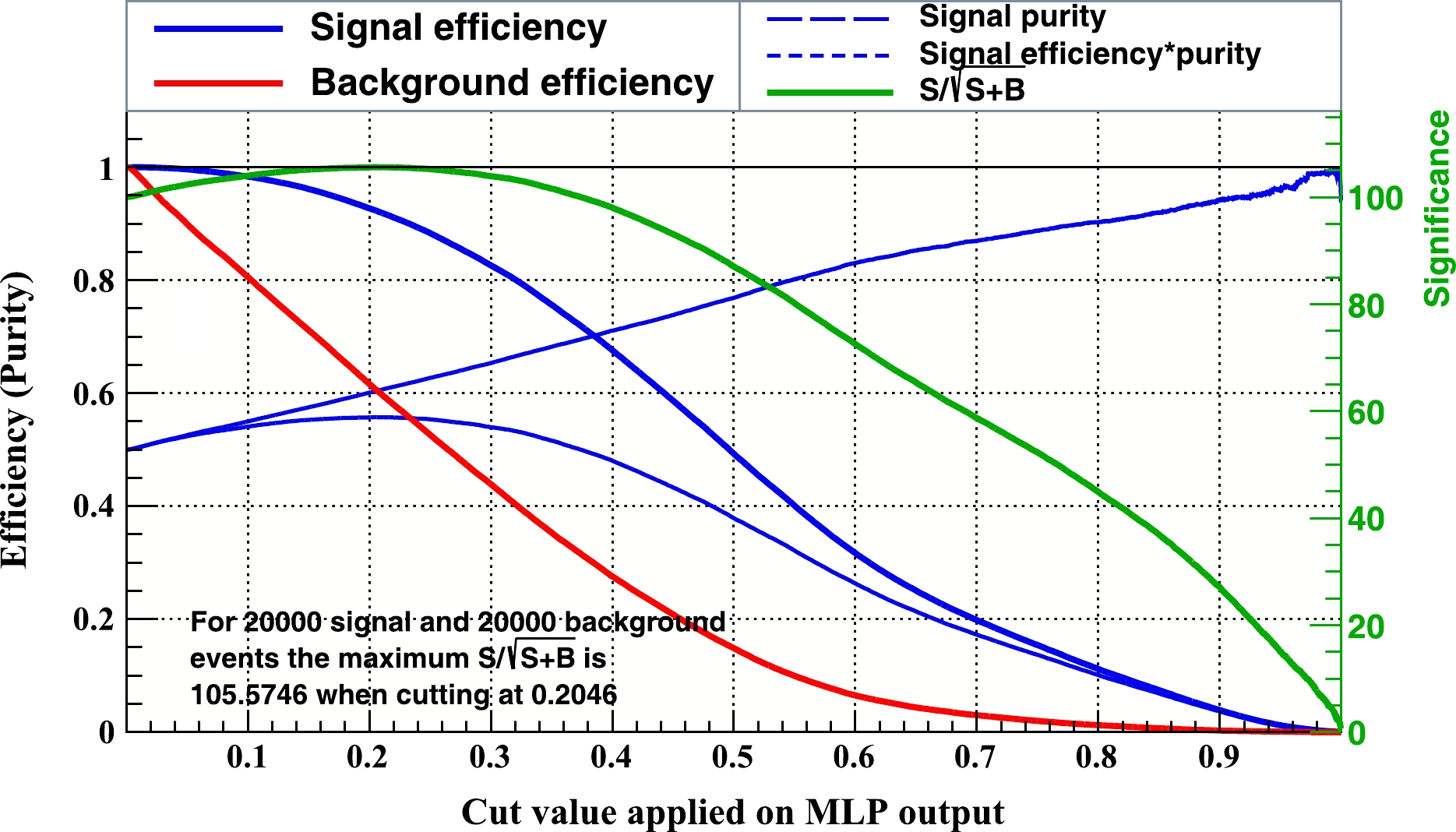
Figure 13. (color online) MLP cut efficiencies as a function of applied cut values.
-
In this study, Type-I 2HDM is used as the theoretical foundation. The selected scenario is similar to the standard model, with the lighter scalar Higgs (h) acting as the SM Higgs boson, in search for a potential discovery channel for the light-
$ H^{+} $ via bosonic decay channels. Bosonic decays of$ H^{+} $ were investigated, as this mode had not been comprehensively explored until now. All$ m_{H^{+}} $ values were set such that they are allowed kinematically. As shown in Fig. 1, when$ m_A $ =$ m_{H^{+}} $ and$\sin(\beta-\alpha)$ is fixed at 0.85, then for$ m_{H^{+}} $ = 400 GeV at 9$\leq \tan\beta \leq 10$ , BR($ H^{+}\rightarrow W^{+}h $ ) is approximately 100%; Fig. 3 shows that for 3$\leq \tan\beta \leq$ 5 and$ m_{H^{+}} $ =160 GeV, a maximum of 20%− 30% of branching ratio is obtained.For larger masses of charged Higgs boson, as shown in Fig. 5, the
$ H^{+}\rightarrow W^{+}A $ decay channel becomes less dominant; however, at 160 GeV and 180 GeV of charged Higgs mass, it becomes dominant when$ m_{A} $ varies between 20 and 120 GeV and$\sin(\beta-\alpha)=0.85$ . For$ m_{H^{+}} $ fixed arbitrarily at 150 GeV, Fig. 8 shows that BR($ H^{+}\rightarrow W^{+}h $ )+BR($ H^{+}\rightarrow W^{+}A $ ) becomes up to 50% observable for$ m_A $ =$ m_{h} $ =125 GeV and$\sin(\beta-\alpha)$ fixed at 0.65. Figure 9 shows that the highest value of σ was obtained for$ m_{H^{+}} $ =150 GeV at 8 TeV, 13 TeV, and 14 TeV of$ \sqrt{s} $ in$ pp $ -collisions. Moreover, by fixing$ m_{H^{+}} $ =150 GeV, Fig. 10 shows that the highest value of σ was obtained at tanβ=2 and the lowest value was obtained at tanβ=20 for the three different values of$ \sqrt{s} $ considered. It was also observed that with an increase in tanβ, the value of the cross-section decreases for$ H^{+}\rightarrow W\phi $ (where ϕ = h or A). Several scans were performed for observing bosonic decay modes of$ H^{\pm} $ from the$[200-1000]\;{\rm GeV}$ mass range and then in a more constrained range of 100−200 GeV. In the next step, for a fixed value of 150 GeV for both decay modes ($ W^{+}h $ ,$ W^{+}A $ ), theoretical and experimental bounds from most recent Higgs searches were applied. Note that it is possible for light$ H^{+} $ to decay via$ H^{+}\rightarrow W^{+}h $ channel or$ H^{+}\rightarrow W^{+}A $ channel (bosonic decay modes). These scans aimed to observe and calculate branching ratios and cross-sections for different bosonic decay modes and compare them with top-bottom decay modes. This study shows that the light charged Higgs boson is possibly observable via bosonic decay channels and points out an alternative discovery channel for this Higgs boson for experimentalists. This study also provides a specific suitable approach to examine beyond standard model (BSM) Higgs bosons as well as validate the sustainability and feasibility of the 2HDM in the selected parameter space.
Observability of parameter space for charged Higgs boson in its bosonic decays in two Higgs doublet model Type-1
- Received Date: 2023-10-28
- Available Online: 2024-02-15
Abstract: This study explores the possibility of discovering


 DownLoad: