Leptonic di-flavor and di-number violation processes at high energy ${{ {\boldsymbol\mu}^{\bf\pm}}{\boldsymbol\mu}^{\bf\pm}} $ colliders

Neutrino oscillations and flavor mixing among the three generations of neutrinos have been observed for years [1]. These phenomena definitely mean that the neutrinos have tiny but nonzero masses and are unambiguous pieces of evidence of new physics (NP) beyond the standard model (SM). Regarding NP, one natural way for neutrinos to acquire tiny masses is through the so-called "seesaw mechanisms" [2]. In these mechanisms, neutrinos, along with the newly introduced heavy neutral leptons, acquire Majorana components, allowing for leptonic di-flavor violation (LFV) processes $ \mu^\pm \mu^\pm \rightarrow e^\pm e^\pm $ and $ \mu^\pm \mu^\pm \rightarrow \tau^\pm \tau^\pm $ and leptonic di-number violation (LNV) processes $ \mu^\pm \mu^\pm \rightarrow W^\pm W^\pm $. Thus, studying these types of same-sign di-lepton and di-boson processes quantitatively to explore how the NP factors (such as the leptonic Majorana components, right handed W-boson, and doubly charged Higgs etc.) play roles is interesting and forms the motivation for this paper. Furthermore, it is known that flavor mixing parameters are strongly constrained by charged lepton flavor violation decays [3−6], whereas the LFV and LNV processes considered in this study may not significantly depend on flavor mixing for the neutral leptons. Therefore, precisely observing the contributions of these mechanisms and NP factors to these processes is particularly intriguing.

Considering the possibility of constructing high energy $ \mu^+ \mu^- $ colliders (e.g., $ \sqrt s\geq 1.0 $ TeV) ¹ [7−10] and the important physics at the high energy colliders, we aim to investigate the important processes at high energy same-sign $ \mu^\pm \mu^\pm $ colliders [11−14]. If there is important physics present at high energy same-sign $ \mu^\pm \mu^\pm $ colliders comparable to that at high energy $ \mu^+\mu^- $ colliders, it is reasonable to consider both of them as potential future options. From the experiences derived from building a proton-antiproton ($ p\bar{p} $) collider (Tevatron) and a proton-proton ($ pp $) collider (LHC), no serious problems should exist for building high energy same-sign $ \mu^\pm \mu^\pm $ colliders in comparison with those for building high energy $ \mu^+ \mu^- $ colliders, provided that the necessary techniques for muon sources, muon acceleration, and muon colliding are developed successfully. Therefore, constructing high energy same-sign $ \mu^\pm \mu^\pm $ collider(s) is a natural extension of building high energy $ \mu^+ \mu^- $colliders, as long as there is sufficient amount of interesting and significant physics to observe. However, fewer studies have investigated the NP of same-sign $ \mu^\pm \mu^\pm $ colliders compared to those focusing on $ \mu^+ \mu^- $ colliders [15−23]. Therefore, in this work, we quantitatively investigate the characteristic processes, LFV processes $ \mu^\pm \mu^\pm \rightarrow e^\pm e^\pm $, $ \mu^\pm \mu^\pm \rightarrow \tau^\pm \tau^\pm $, and LNV processes $ \mu^\pm \mu^\pm \rightarrow W^\pm _iW^\pm _j $ ($ i,\;j=1,\;2 $) at high energy same-sign muon colliders.

The process $ e^\pm e^\pm \rightarrow \mu^\pm \mu^\pm $ was studied in Ref. [24], and the authors presented the theoretical predictions with the minimal type-I seesaw mechanism and analyzed the contributions from the supersymmetric particles. In Refs. [25−27], the contributions from the doubly charged Higgs to the process $ e^\pm e^\pm \to \mu^\pm \mu^\pm $ were also examined. Studies of the LNV di-boson process $ e^\pm e^\pm \to W_L^\pm W_L^\pm $ were reported in Refs. [28−39]. Theoretical predictions on the cross sections of $ e^\pm e^\pm \to W_L^\pm W_L^\pm $, $ e^\pm e^\pm \rightarrow W_L^\pm W_R^\pm $ in the left-right symmetric model (LRSM) were presented in Refs. [40−43]. In this work, we investigate the NP contributions to the LFV di-lepton and LNV di-boson processes and explore their phenomenological behaviors at high energy $ \mu^\pm \mu^\pm $ colliders. It is worth noting that the contributions to the LFV and LNV processes from the e-flavor heavy neutral lepton are significantly constrained by the recent experimental upper bound on the $ 0\nu2\beta $ decay half-life. This is because the "core" process of $ 0\nu2\beta $ decays is $ d+d\rightarrow u+u+e+e $; that is, all the processes with $ e^\pm e^\pm $ being in the initial state are also constrained by the $ 0\nu2\beta $ experiments [44].

In this study, we mainly focus on exploring the sources of NP that generate the LFV di-lepton and LNV di-boson processes, namely, a) the neutral leptons' Majorana components with the help of the left-handed $ W_L $boson only or with the help of both the left-handed and right-handed bosons $ W_L $ and $ W_R $ , respectively, and b) the doubly charged Higgs and the interference effects of the Higgs and neutral leptons' Majorana components ². To explore the phenomena of the NP factors and their combinations, we categorize them into three types: Type I of NP (TI-NP), such as the $ B-L $ symmetric SUSY model (B-LSSM) [45−48], which involves the combination of neutral leptons' Majorana components and the left-handed $ W_L $ boson; Type II of NP (TII-NP), such as the left-right symmetric model (LRSM) without doubly charged Higgs, which involves the combination of neutral leptons' Majorana components, the left-handed boson $ W_L $, and the right-handed boson $ W_R $; Type III of NP (TIII-NP), such as the LRSM [49−55], which encompasses the presence of doubly charged Higgs alongside the $ W_L $ and $ W_R $ bosons and neutral leptons' Majorana components. The behaviors of the LFV di-lepton and LNV di-boson processes at high energy $ \mu^\pm \mu^\pm $ colliders resulting from these three types of NP will be computed and discussed in this paper.

The paper is organized as follows: in Sec. II, the seesaw mechanisms giving rise to the heavy neutral lepton masses, tiny neutrino masses, relevant Majorana components, and interaction vertices are outlined for later applications. In Sec. III, the theoretical computations of the processes $ \mu^\pm \mu^\pm \rightarrow l^\pm l^\pm \;(l=e,\;\tau) $ and $\mu^\pm \mu^\pm \rightarrow W^\pm _i W^\pm _j$ ($ i,\;j=1,\;2 $) for the three types of NP are presented. In Sec. IV, the numerical results with suitable input parameters, which are constrained by the available experiments, are calculated and presented by figures. Finally, in Sec. V, the results are discussed and a summary is provided.

In this section, we briefly review the mechanisms that make the neutrinos acquire tiny masses and mixtures. Furthermore, we outline the necessary interactions that relate to the three types of NP and are required for the computation of the LFV di-lepton and LNV di-boson processes.

First, as representative of TI-NP, let us consider the B-LSSM. Its gauge group is extended by adding a local group $ U(1)_{B-L} $ to the SM, where B and L represent the baryon number and lepton number, respectively. In this model, three right-handed neutral leptons and two singlet scalars (Higgs), possessing a non-zero $ B-L $ charge, are introduced. The Majorana masses of the right-handed neutral leptons arise when the two singlet scalars (Higgs) acquire vacuum expectation values (VEVs). Combining the Majorana mass terms with the Dirac mass terms, tiny neutrino masses can be obtained by the type-I seesaw mechanism. Thus, the mass matrix of neutral leptons reads

where $ M_D $ is the Dirac mass matrix of $ 3 $ by $ 3 $, and $ M_R $ is the Majorana mass matrix of $ 3 $ by $ 3 $. We can define $ \xi_{ij}=(M_D^TM_R^{-1})_{ij} $; then, the mass matrix in Eq. (1) can be diagonalized approximately as

where $ \hat m_\nu={\rm diag}(m_{\nu_1},m_{\nu_2},m_{\nu_3}) $ with $ m_{\nu_i}\;(i=1,\;2,\;3) $ denoting the $ i- $th generation of light neutrino masses, $ \hat M_N={\rm diag}(M_{N_1},M_{N_2},M_{N_3}) $, with $ M_{N_i}\;(i=1,\;2,\;3) $ denoting the $ i- $th generation of heavy neutral lepton masses, and

Then, we have

In the following analysis, the $ 3 $ by $ 3 $ matrix U is taken as the Pontecorvo-Maki-Nakagawa-Sakata (PMNS) mixing matrix, which is measured from the neutrino oscillation experiments. The relevant Lagrangian for the $ l-W-\nu $ and $ l-W-N $ ($ l=e,\mu,\tau $) interactions in the model becomes

where $ P_{L,R}=(1\mp\gamma^5)/2 $, and $ \nu,\;N $ are the four-component forms of mass eigenstates corresponding to light and heavy neutral leptons, respectively. The LFV di-lepton processes will be calculated in the Feynman gauge later on; hence, the $ l-G-\nu $ and $ l-G-N $ interactions where G denotes the Goldstone boson occur, and the relevant Lagrangian is written as

where $ U,\;S,\;T,\;V $ are matrices of $ 3 $ by $ 3 $ defined in Eq. (3); $ \hat m_l={\rm diag}(m_{e},m_{\mu},m_{\tau}) $, with $ m_{e},m_{\mu},m_{\tau} $ denoting the charged lepton masses; $ G_L $ is the goldstone boson which is "eaten" by $ W_L $ in unitary gauge; and $ M_{W_L} $ is the $ W_L $ boson mass. Having the relevant Lagrangian $ \mathcal{L}_{W}^{BL} $ and $ \mathcal{L}_{G}^{BL} $, the theoretical predictions of the considered processes for TI-NP can be calculated.

As representative of TII-NP and TIII-NP, let us consider the left-right symmetric model (LRSM). Its gauge group is $S U(3)_C\bigotimes S U(2)_L\bigotimes S U(2)_R\bigotimes U(1)_{B-L}$. The additional three generations of the right-handed neutral leptons which with the three generations of the right-handed charged leptons form doublets, the di-doublet scalar (Higgs), and the two triplet scalars (Higgs)

are involved, and $ v_1,\;v_2,\;v_L,\;v_R $ are the VEVs of $ \phi_1^0,\;\phi_2^0,\;\Delta_{L}^0,\;\Delta_{R}^0 $, respectively. The Yukawa Lagrangian for the lepton sector is given by

where the family indices $ i,\;j $ are summed over, and $ \tilde \Phi= \sigma^2\Phi^*\sigma^2 $. The tiny neutrino masses are obtained by both the type-I and type-II seesaw mechanisms when the Higgs $ \phi_1^0,\;\phi_2^0,\;\Delta_{L}^0,\;\Delta_{R}^0 $ achieve VEVs [49−53]. Then, the mass matrix of neutral leptons can be written as

where

The Lagrangian for the $l^{-}-\Delta^{-\;\;-}_{L,R}-l^-$ interactions is

The mass matrix in Eq. (9) can be diagonalized in terms of a unitary matrix $ U_\nu $, whereas the matrix $ U_\nu $ can be expressed similarly as that in the above case of the B-LSSM, Eq. (3). Then, we can obtain [44]

The second formula in Eq. (12) is obtained by using the approximation $ M_R^{-1}M_D^*M_D^T\approx M_DM_D^\dagger M_R^{-1}\ll M_R $. Because of the $S U(2)_R$ gauge group, there are charged right-handed gauge bosons $ W^\pm_R $ additionally, and the two types of bosons $ W_L $ and $ W_R $ may be mixed. As the result of $ W_L-W_R $ mixing, the masses of the physical $ W_1 $ (dominated by the left-handed $ W_L $) and $ W_2 $ (dominated by the right-handed $ W_R $) can be written as follows [44]:

Then, the Lagrangian for the $ l-W-\nu $ and $ l-W-N $ interactions for the LRSM is

where $ \tan2\zeta=\dfrac{2v_1v_2}{v_R^2-v_L^2} $ denotes the mixing between $ W_L $ and $ W_R $, the matrices $ U,\;S,\;T,\;V $ are defined in Eq. (3), and $ \nu,\;N $ are the four-component fermion fields of the mass eigenstates corresponding to light and heavy neutral leptons, respectively. The Lagrangian for the $ l-G-\nu $ and $ l-G-N $ interactions may be written as [49]

where $ G_L, G_R $ are the unphysical Goldstone bosons when the Feynman gauge is applied ³, and

Finally, the relevant Lagrangian for the $ W-\Delta^{-}_{L,R}-W $ interactions is

Hence, the theoretical predictions of the considered processes for TII-NP can now be calculated based on the Lagrangian $ \mathcal{L}_{W}^{LR} $, $ \mathcal{L}_{G}^{LR} $, and those for TIII-NP can be calculated based on the Lagrangian $ \mathcal{L}_{\Delta ll}^{LR} $, $ \mathcal{L}_{W}^{LR} $, $ \mathcal{L}_{G}^{LR} $, $ \mathcal{L}_{\Delta WW}^{LR} $.

Note that there is a possible model containing doubly charged Higgs in its scalar triplet with Type-II seesaw [56−59], and the doubly charged component of the triplet Higgs can also cause the LFV and LNV processes. However, the contributions to the processes (which are much smaller than those considered here) are highly suppressed as the relevant interactions are proportional to the light neutrino masses. Thus, the contributions to the LFV and LNV processes from the three types of NP considered here are much greater, and thus, we will not discuss this model here.

In this section we will provide the calculations of the processes $ \mu^\pm \mu^\pm \rightarrow l^\pm l^\pm \;(j=e,\;\tau) $, $ \mu^\pm \mu^\pm \rightarrow W^\pm _i W^\pm _j\;(i,j=1,2) $ within TI-NP, TII-NP, and TIII-NP. The results for TI-NP and TII-NP can be obtained by switching off certain interactions from the relevant results for TIII-NP. In all the computations, the flavor mixing parameters of the heavy neutral leptons are ignored because the flavor mixing parameters are strongly constrained by the charged lepton flavor violating decays [3−6].

The leading-order Feynman diagrams for the LFV di-lepton processes $ \mu^\pm \mu^\pm \rightarrow l^\pm l^\pm \;(l=e,\;\tau) $ incorporating the contributions from Majorana neutral leptons in TI-NP, TII-NP, and TIII-NP are collected in Fig. 1. However, in the case of TI-NP, the Feynman diagrams with $ W_2 $ and/or $ G_R $ line(s) should be moved away. Note that here, for simplification, the Feynman diagrams with the gauge boson $ W_{1,2} $ lines and/or Goldstone boson $ G_{L,R} $ lines crossed are not presented in the figure. In fact, the contributions from these crossing diagrams to the processes should be well taken into account. Hence, when doing the calculations, we do consider the contributions from these crossing diagrams.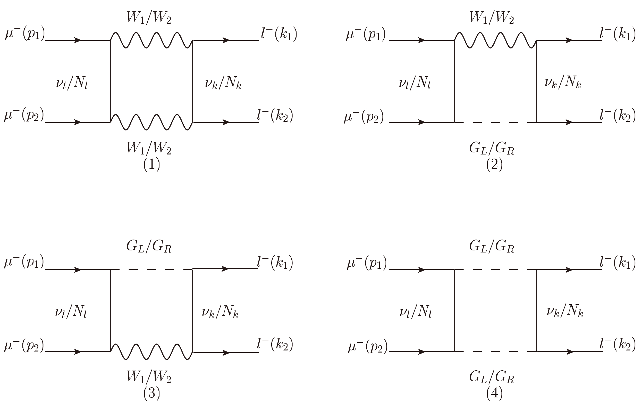

Figure 1.  Feynman diagrams (leading order) in Feynman gauge for the $ \mu^- \mu^- \rightarrow l^- l^- \;(l=e,\;\tau) $ processes via neutrino and neutral heavy lepton exchanges.

The mixing parameter ζ between the left-handed boson $ W_L $ and the right-handed boson $ W_R $ is constrained in the range $ \zeta\lesssim7.7\times10^{-4} $ [60], and the charged lepton masses are much smaller than the center-of-mass energy of the collisions. Thus, in the calculations, we ignore the contributions proportional to $ \mathcal{O}(\zeta^2) $ and charged lepton masses. Then, the amplitude of the processes $ \mu^\pm \mu^\pm \rightarrow l^\pm l^\pm $ for TIII-NP can be formulated as

where

where u is the Dirac spinor of the leptons, $ u^c\equiv C\bar u^T $ is its charge conjugation, the charge conjugation operator $C\equiv {\rm i}\gamma_2\gamma_0$, and $ \gamma_{0},\;\gamma_{2} $ are the Dirac matrices. The momenta $ p_1,p_2,k_1,k_2 $ are defined as shown in Fig. 1, and the coefficients $ C_i^{XY} $ in Eq. (18) can be read out from the amplitudes relating to the Feynman diagrams in Fig. 1.

To show how the coefficients are read out, now let us take the Feynman diagram in Fig. 1 (1) as an example, where $ \nu_{k} $, $ \nu_{l} $, $ W_1 $, $ W_2 $ appear in the loop. According to the interactions in Sec. II, the amplitude can be written as

where $ \Gamma_{W_1},\;\Gamma_{W_2} $ are the total decay widths of $ W_1,\;W_2 $ bosons, respectively. The integrals appearing in Eq. (20) can be calculated by using Loop-Tools [61, 62]. Hence, for the further calculations, we define the functions following the conventions in Loop-Tools as

where $ l_1,\;l_2,\;l_3 $ are combinations of out-leg particles' momentum (for example, for the loop integral in Eq. (20), we may have $ l_1=k_1-p_1,\;l_2=-p_1,\;l_3=p_2 $); q is the integral momentum, $m_i^2\equiv M_i^2-{\rm i}\Gamma_i M_i$, with $ M_i $ and $ \Gamma_i $ denoting the mass and total decay width of loop particle i, respectively; and

According to the definitions in Eq. (21), the amplitude $ \mathcal{M}(\nu\nu W_1W_2) $ can be simplified by neglecting the tiny neutrino mass terms in the numerators of the neutrino propagators and the terms proportional to charged lepton masses that appear after applying the on-shell condition for the leptons. Then, the amplitude $ \mathcal{M}(\nu\nu W_1W_2) $ finally becomes

where $ D_{00},\;D_{0},\;D_{1},\;D_{2},\;D_{12} $ can be computed numerically by using Loop-Tools. Then, from $ \mathcal{M}(\nu\nu W_1W_2) $, the coefficients $ C_i^{XY} $ of $ \mathcal{O}_i^{XY}\;(i=1,...,7) $, defined in Eq. (19), can be read out as

This is, corresponding to the amplitude for the Feynman diagram in Fig. 1 (1), only the coefficients $ C_1^{LL} $ and $ C_2^{LL} $ receive nonzero contributions. When we calculate the other Feynman diagrams in Fig. 1, where the two outgoing charged leptons l ($ l=e,\;\tau $) of the Feynman diagrams are alternated, the identity formulas

are applied to $ \mathcal{O}_i^{XY}\,(i=1,...,7) $, as defined in Eq. (19). Because each of the amplitudes of the above Feynman diagrams may be treated in the same way as that in Fig. 1 (1), all the coefficients $ C_i^{XY} $ in Eq. (18) for the relevant processes may be obtained.

The contributions from doubly charged Higgs ($ \Delta^{\pm \pm} $) to the LFV di-lepton processes $ \mu^\pm \mu^\pm \rightarrow l^\pm l^\pm \;(l=e,\;\tau) $ can be estimated from the Feynman diagram in Fig. 2. The amplitude corresponding to Fig. 2 can be formulated as in Eq. (18), and the nonzero coefficients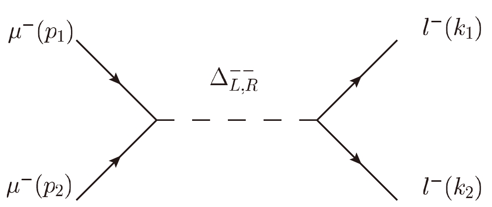

Figure 2.  Feynman diagrams for $ \mu^\pm \mu^\pm \rightarrow l^\pm l^\pm \;(l=e,\;\tau) $ due to doubly charged Higgs.

are left, where $ j=e,\;\tau $, $ \Gamma_{\Delta_{L,R}^{-}} $ is the total decay width of the Higgs $ \Delta_{L,R}^{-} $.

Based on the total amplitude formulated as Eq. (18), the amplitude can be squared absolutely by summing up the lepton spins in the initial and final states. Neglecting the charged lepton masses from the square of $ \mathcal{O}_i^{XY}\, (i=1,...,7) $, i.e., those in Eq. (19), the result can be simplified as

Now, the cross section of LFV di-lepton processes can be written as

where the factor $ \frac{1}{4} $ results from averaging the lepton spins in the initial state, θ is the angle between the direction of the outgoing lepton l with the collision axis, and $ \sqrt s $ is the total collision energy of $ \mu^\pm \mu^\pm $ colliders.

The Feynman diagrams contributing to the LNV processes $ \mu^\pm \mu^\pm \rightarrow W_i^\pm W_j^\pm, i,j=1,2 $ at the tree-level are plotted in Fig. 3, where the final sates $ W_i^\pm W_j^\pm $ denote $ W_1^\pm W_1^\pm $ or $ W_1^\pm W_2^\pm $ or $ W_2^\pm W_2^\pm $. Summing up the fermions' spin and gauge bosons' polarizations, the squared amplitude for the processes $ \mu^\pm \mu^\pm \rightarrow W_i^\pm W_j^\pm $ can be simplified by neglecting the terms proportional to $ \mathcal{O}(\sin^2\zeta) $ and the charged lepton mass $ m_\mu $ as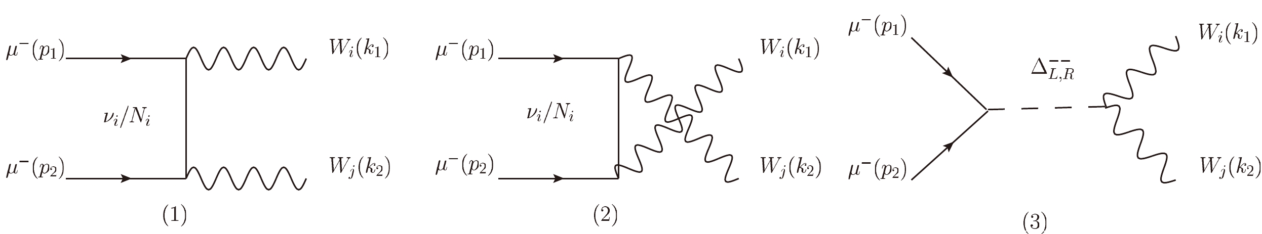

Figure 3.  Feynman diagrams for the LNV processes $ \mu^\pm \mu^\pm \rightarrow W_i^\pm W_j^\pm $ as those in the LRSM: Figs. 1 and 2 are related to the neutral Majorana lepton contributions, and Fig. 3 is related to the doubly charged Higgs contributions. Here, the final sates $ W_i^\pm W_j^\pm $ denote $ W_1^\pm W_1^\pm $, $ W_1^\pm W_2^\pm $ , or $ W_2^\pm W_2^\pm $.

where

Note that the mixing parameter $ \sin \zeta $ is not present in Eqs. (31)−(33). This is because, in the calculations of the further approximation, the contributions up-to $ \mathcal{O}(\sin\zeta) $ are maintained, and the mass of the initial charged lepton is set to be zero. This approximation also disregards the contributions of doubly charged Higgs $ \Delta_{L,R}^{\pm\pm} $ to the process $ \mu^\pm\mu^\pm\rightarrow W_1^\pm W_2^\pm $. For TIII-NP, Eq. (31) and Eq. (33) show that $ \Delta_L^{\pm\pm} $ primarily contributes to the process $ \mu^\pm \mu^\pm \to W_1^\pm W_1^\pm $, whereas $ \Delta_R^{\pm\pm} $ primarily contributes to the process $ \mu^\pm \mu^\pm \to W_2^\pm W_2^\pm $. Consequently, the distinct characteristics of $ \Delta_L^{\pm\pm} $ and $ \Delta_R^{\pm\pm} $ can be identified by observing the LNV di-boson processes at $ \mu^\pm\mu^\pm $ colliders.

The results of $ \mu^\pm\mu^\pm\to W_L^\pm W_L^\pm $ for TI-NP can be acquired by setting $ Y_{L,22}=0 $ in Eq. (31), and the results of $ \mu^\pm\mu^\pm\to W_1^\pm W_1^\pm $, $ \mu^\pm\mu^\pm\to W_1^\pm W_2^\pm $, and $ \mu^\pm\mu^\pm\to W_2^\pm W_2^\pm $ for TII-NP can be acquired by setting $ Y_{L,22}=Y_{R,22}=0 $ in Eqs. (31) and (33). Based on the computations of the LNV di-boson processes, one may realize that the results of the $ \mu^\pm\mu^\pm\to W_1^\pm W_1^\pm $ cross section for TII-NP are similar to those of the $ \mu^\pm\mu^\pm\to W_L^\pm W_L^\pm $ cross section for TI-NP, and the results of the $ \mu^\pm\mu^\pm\rightarrow W_1^\pm W_2^\pm $ cross section for TIII-NP are similar to those of the $ \mu^\pm\mu^\pm\rightarrow W_1^\pm W_2^\pm $ cross section for TII-NP. The cross sections of LNV di-boson processes can be written as

where the factor $ \dfrac{1}{4} $ results from averaging the lepton spins in the initial state, and θ is the angle between the momentum of the outgoing $ W_i $ and the collision axis. Considering the phase space integration factor of the identified particles, $ A=2 $ for $ W_iW_j=W_1W_1,\;W_2W_2 $ and $ A=1 $ for $ W_iW_j=W_1W_2 $.

In this section, we will calculate numerical results for the cross sections of the LFV and LNV processes associated with TI-NP, TII-NP, and TIII-NP, using the formulas derived in Sec. III. To carry out the numerical evaluations, numerous parameters in the NP that are constrained by the available experiments need to be fixed. Thus, let us explain how the parameters are fixed. The PDG [1] have collected a large number of parameters such as $ M_{W_L}(M_{W_1})=80.385\;{\rm GeV} $, $ \Gamma_{W_L}=2.08\;{\rm GeV} $, $\alpha_{em}(m_Z) = 1/128.9$, and the charged lepton masses $ m_e=0.511\;{\rm MeV},\; m_\mu=0.105\;{\rm GeV},\;m_\tau=1.77\;{\rm GeV} $, among others, and we adopt them all. The sum of neutrino masses is limited in the range $ \sum\limits_i m_{\nu i}<0.12\;{\rm eV} $ by Plank [63]. This indicates that the contributions of the neutrino mass terms are negligible, regardless of whether the neutrino masses are in normal hierarchy ($ m_{\nu_1}<m_{\nu_2}<m_{\nu_3} $) or inverse hierarchy ($ m_{\nu_3}<m_{\nu_1}<m_{\nu_2} $). Hence, we will ignore the contributions proportional to neutrino masses in the numerical evaluations. The matrix U (the upper-left sub-matrix of the whole matrix $ U_\nu $ in Eq. (3)) is taken as the PMNS mixing matrix [1] to describe the mixing of the light neutrinos.

For the light-heavy neutral lepton mixing (LHM) matrix $ S_{ij} $, we set $ S_{i}^2\equiv\sum\limits_{j}|S_{ij}|^2\;(i,j=e,\mu,\tau) $ to describe the strength of the LHM. The direct constraint on $ S_{e}^2 $ comes from the $ 0\nu2\beta $ decay searches as $ S_e^2\lesssim 10^{-5} $ [44]. The direct constraint on $ S_\mu^2 $ is given by CMS as $ S_\mu^2\lesssim 0.4 $ for TeV-scale heavy neutral lepton masses [64−66]. Recently, the constraint on $ S_\mu^2 $ from the future high-luminosity Large Hadron Collider (HL-LHC) was analyzed in Ref. [67], and the authors claim that $ S_\mu^2\lesssim 0.06 $ for TeV-scale heavy neutral lepton masses. There is no direct constraint presently on $ S_\tau^2 $ for TeV-scale heavy neutral lepton masses. In the following analysis, we will show that the proposed $ \mu^\pm\mu^\pm $ colliders are more sensitive to $ S_\mu^2 $, $ S_\tau^2 $ than the LHC and future HL-LHC for TeV-scale heavy neutral lepton masses. Hence, we set

Here, $ S_\mu^2 $ and $ S_\tau^2 $ are set to a smaller value than that the HL-LHC can reach.

Considering the direct observations on the right-handed weak gauge boson $ W_R $ ($ W_2 $), the lower bound for the mass of the $ W_2 $ boson reads $ M_{W_2}\gtrsim4.8\;{\rm TeV} $ [68−71], and its total decay width can be approximately estimated as $ \Gamma_{W_2}\approx0.028 M_{W_2} $ [52]. On the doubly charged Higgs masses, the most recent limits from the LHC [72, 73] are $ M_{\Delta_{L}^{\pm\pm}}\gtrsim800\;{\rm GeV},\;M_{\Delta_{R}^{\pm\pm}}\gtrsim650\;{\rm GeV} $. As pointed out above, the signals of $ \Delta_L^{\pm\pm} $ and $ \Delta_R^{\pm\pm} $ produced in the LFV di-lepton and LNV di-boson processes at $ \mu^\pm\mu^\pm $ colliders can be used to identify them, and the signatures may well show their mass and width accordingly. According to Refs. [74−77], the total decay widths of $ \Delta_L^{\pm\pm} $ and $ \Delta_R^{\pm\pm} $ can be written as

where

and

The relevant Yukawa coupling $ Y_{R,ll} $ is not a free parameter ⁴; therefore, we only have the Yukawa coupling $ Y_L $ of the left-handed doubly charged Higgs to the leptons that need to be set. Generally, it takes the following formulation:

$ Y_{ee} $ is strongly constrained by the $ 0\nu2\beta $ decay experiments in the range $ Y_{ee}\lesssim0.04 $. In addition, a small VEV $ v_L $ of $ \Delta_L^0 $, $ v_L\lesssim 5.0\;{\rm GeV} $, is constrained by the $ \rho- $parameter [1]. Thus, we will set it as $ v_L=0.1\;{\rm GeV} $ to simplify the numerical evaluations.

In this subsection, the numerical results related to the LFV di-lepton processes $ \mu^\pm\mu^\pm\to e^\pm e^\pm $ and $ \mu^\pm\mu^\pm\to \tau^\pm \tau^\pm $ for TI-NP, TII-NP, and TIII-NP are presented. The characteristics of the LFV di-lepton processes are clear and practically free from SM background processes at high energy same-sign muon colliders [26] ⁵. First, let us focus lights on the effects of LHM parameter $ S_\mu^2 $ and the heavy neutral lepton mass $ M_{N_2} $.

Taking the possible $ M_{N_1}=1.0\;{\rm TeV} $, $ M_{N_3}=3.0\;{\rm TeV} $, $ S_e^2=10^{-5},\;S_\tau^2=10^{-2} $, $ \sqrt s=5.0\;{\rm TeV} $ as an example, we present the results of $ \sigma(\mu^\pm\mu^\pm\rightarrow \tau^\pm\tau^\pm) $ and $ \sigma(\mu^\pm\mu^\pm\rightarrow e^\pm e^\pm) $ versus $ S_\mu^2 $ in Fig. 4 (a) and Fig. 4 (b), respectively, where the solid, dashed, and dotted curves denote the results for $ M_{N_2}=1.0,\;2.0,\;3.0\; $ TeV, respectively. In the figures, the black curves denote the results for TI-NP, the red curves denote the results for TII-NP with $ M_{W_2}= $ 5.0 TeV, and the blue curves denote the results for TIII-NP with $ M_{W_2}= $ 5.0 TeV, $ M_{\Delta_L^{\pm\pm}}=10.0\; $TeV, $ M_{\Delta_R^{\pm\pm}}=11.0\; $TeV, $ Y_{ee}=0.04 $, $ Y_{\mu\mu}=1.0 $, and $ Y_{\tau\tau}=1.0 $. Note here that the masses of the heavy neutral leptons are set at the TeV scale because it is challenging to exclude them by experiments in the near future. We additionally attempt to set $ \sqrt s=5.0\;{\rm TeV} $ as a representative collision energy for TeV scale $ \mu^\pm\mu^\pm $ colliders in Fig. 4, and the numerical results for various $ \sqrt s $ values are investigated in Fig. 5.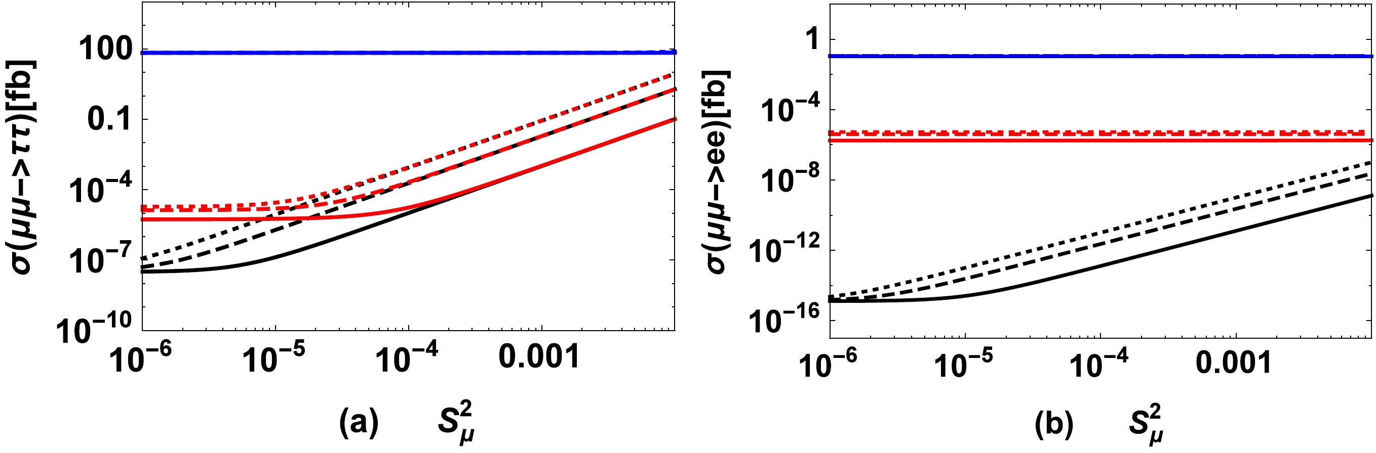

Figure 4.  (color online) Cross-section $ \sigma(\mu^\pm\mu^\pm\rightarrow l^\pm l^\pm) $ versus $ S_\mu^2 $ for $ M_{N_1}=1.0\;{\rm TeV} $, $ M_{N_3}=3.0\;{\rm TeV} $, $ S_e^2=10^{-5},\;S_\tau^2=0.01 $, and $ \sqrt s=5.0\;{\rm TeV} $. In (a), $ l=\tau $, and in (b), $ l=e $. The solid, dashed, and dotted curves denote the results for $ M_{N_2}=1.0,\;2.0,\;3.0\; $TeV, respectively. The black curves denote the results for TI-NP, the red curves denote the results for TII-NP with $ M_{W_2}=5.0\;{\rm TeV} $, and the blue curves denote the results for TIII-NP with $ M_{W_2}=5.0\;{\rm TeV} $, $ M_{\Delta_L^{\pm\pm}}=10.0\; $TeV, $ M_{\Delta_R^{\pm\pm}}=11.0\; $TeV, $ Y_{ee}=0.04 $, $ Y_{\mu\mu}=1.0 $, and $ Y_{\tau\tau}=1.0 $.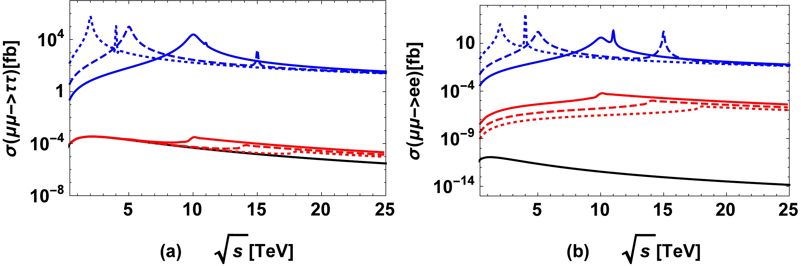

Figure 5.  (color online) $ \sigma(\mu^\pm\mu^\pm\to l^\pm l^\pm) $ versus $ \sqrt s $ with $ M_{N_1}=1.0\;{\rm TeV} $, $ M_{N_2}=2.0\;{\rm TeV} $, $ M_{N_3}=3.0\;{\rm TeV} $, $ S_e^2=10^{-5} $, $ S_\mu^2=10^{-4} $, and $ S_\tau^2=10^{-2} $. In (a), $ l=\tau $, and in (b), $ l=e $. The black curves denote the results for TI-NP, and the red curves denote the results for TII-NP. The red solid, red dashed, and red dotted curves denote the results for $ M_{W_2}=5.0,\;7.0,\;9.0\; $TeV, respectively. The blue curves denote the results for TIII-NP with $ M_{W_2}=5.0\; $TeV, $ Y_{ee}=0.04 $, $ Y_{\mu\mu}=1.0 $, and $ Y_{\tau\tau}=1.0 $. The blue solid curves denote the results for $ M_{\Delta_L^{\pm\pm}}=10.0\; $TeV and $ M_{\Delta_R^{\pm\pm}}=11.0\; $TeV, the blue dashed curves denote the results for$ M_{\Delta_L^{\pm\pm}}=5.0\; $TeV and $ M_{\Delta_R^{\pm\pm}}=15.0\; $TeV, and the blue dotted curves denote the results when setting$ M_{\Delta_L^{\pm\pm}}=2.0\; $TeV and $ M_{\Delta_R^{\pm\pm}}=4.0\; $TeV.

The numerical results in Fig. 4 indicate that when an integrated luminosity of $ 500\;{\rm fb}^{-1} $ is accumulated at a TeV scale $ \mu^\pm \mu^\pm $ collider, the process $ \mu^\pm\mu^\pm\rightarrow \tau^\pm \tau^\pm $ predicted by TI-NP, TII-NP and the processes $ \mu^\pm\mu^\pm\rightarrow \tau^\pm \tau^\pm $, $ \mu^\pm\mu^\pm\rightarrow e^\pm e^\pm $ predicted by TIII-NP have great opportunities to be observed. Because their cross sections can be larger than $ 0.1\;{\rm fb} $ in a reasonably selected parameter space, more than $ 50 $ signal events/year can be collected. This indicates that the $ \mu^\pm\mu^\pm $ collider is more sensitive to $ S_\mu^2 $ and $ S_\tau^2 $ than the future HL-LHC. The contributions from Majorana neutral leptons to $ \sigma(\mu^\pm\mu^\pm\rightarrow \tau^\pm \tau^\pm) $, $ \sigma(\mu^\pm\mu^\pm\rightarrow e^\pm e^\pm) $ are proportional to $ S_\mu^2 S_\tau^2 $, $ S_\mu^2 S_e^2 $, respectively. Further, the contributions from the doubly charged Higgs to $ \sigma(\mu^\pm\mu^\pm\rightarrow \tau^\pm \tau^\pm) $, $ \sigma(\mu^\pm\mu^\pm\rightarrow e^\pm e^\pm) $ are proportional to $ Y_{\mu\mu}Y_{\tau\tau} $, $ Y_{\mu\mu}Y_{ee} $, respectively. Moreover, $ S_e^2 $ and $ Y_{ee} $ are constrained to be small by the $ 0\nu2\beta $ experiments, whereas $ S_\tau^2 $ and $ Y_{\tau\tau} $ are not, and therefore, the contributions to $ \sigma(\mu^\pm\mu^\pm\rightarrow e^\pm e^\pm) $ are comparatively. This fact can be clearly realized by comparing Fig. 4 (a) with Fig. 4 (b). From the figures, it can be found that the three blue curves merge together in the logarithmic coordinate, and the predicted cross sections $ \sigma(\mu^\pm \mu^\pm \rightarrow \tau^\pm \tau^\pm) $ and $ \sigma(\mu^\pm \mu^\pm \to e^\pm e^\pm) $ for TIII-NP are much larger than those predicted by TI-NP and TII-NP. This occurs because the leading contributions to the LFV di-lepton processes for TIII-NP come from the $ s $-channel mediation of the doubly charged Higgs at the tree level, whereas those for TI-NP and TII-NP start with the one-loop level, which involves the Majorana neutral leptons. The black and red curves in Fig. 4 (a), (b) show that $ \sigma(\mu^\pm \mu^\pm \rightarrow \tau^\pm \tau^\pm) $ and $ \sigma(\mu^\pm \mu^\pm \rightarrow e^\pm e^\pm) $ are dominated by right-handed gauge boson for TII-NP if $ S_l^2 $ ($ l=e,\;\mu,\;\tau $) are small. The results of $ \sigma(\mu^\pm \mu^\pm \to \tau^\pm \tau^\pm) $ for TI-NP, TII-NP are similar when $ S_\mu^2\gtrsim 10^{-4} $, and $ \sigma(\mu^\pm \mu^\pm \to e^\pm e^\pm) $ for TII-NP is always larger than that for TI-NP owing to the fact that only the contributions from $ W_L $ mediation exist for TI-NP. The contributions to the LFV di-lepton processes for TIII-NP are dominated by the doubly charged Higgs, and hence, the dependence on $ S_l^2 $ may be ignorable. A large $ M_{N_2} $ plays an enhancing role on $ \sigma(\mu^\pm \mu^\pm \to \tau^\pm \tau^\pm) $ and $ \sigma(\mu^\pm \mu^\pm \to e^\pm e^\pm) $ for TI-NP and TII-NP. This occurs because the goldstone component (in Feynman gauge) makes dominant contributions to the LFV di-lepton processes for TI-NP and TII-NP, and the corresponding couplings increase with the increasing of heavy neutral lepton masses for a given $ S_l^2 $.

The results of $ \sigma(\mu^\pm\mu^\pm\to \tau^\pm\tau^\pm) $ and $ \sigma(\mu^\pm\mu^\pm\to e^\pm e^\pm) $ versus $ \sqrt s $ are presented in Fig. 5 (a) and Fig. 5 (b), respectively, for $ M_{N_1}=1.0\;{\rm TeV} $, $ M_{N_2}=2.0\;{\rm TeV} $, $ M_{N_3}= $ 3.0 TeV, $ S_e^2=10^{-5} $, $ S_\mu^2=10^{-4} $, and $ S_\tau^2=10^{-2} $. The black curves denote the results for TI-NP. The red curves denote the results for TII-NP, where the red solid, red dashed, and red dotted curves denote the results when $ M_{W_2}=5.0,\;7.0,\;9.0\; $ TeV, respectively. The blue curves denote the results for TIII-NP with possible parameters $ M_{W_2}=5.0\; $TeV, $ Y_{ee}=0.04 $, $ Y_{\mu\mu}=1.0 $, and $ Y_{\tau\tau}=1.0 $, where the blue solid curves denote the results with $ M_{\Delta_L^{\pm\pm}}=10.0\; $TeV and $ M_{\Delta_R^{\pm\pm}}=11.0\; $TeV, the blue dashed curves denote the results with $ M_{\Delta_L^{\pm\pm}}=5.0\; $TeV and $ M_{\Delta_R^{\pm\pm}}=15.0\; $TeV, and the blue dotted curves denote the results with $ M_{\Delta_L^{\pm\pm}}=2.0\; $TeV and $ M_{\Delta_R^{\pm\pm}}=4.0\; $ TeV. As for TIII-NP, the contributions to the LFV di-lepton processes are dominated by doubly charged Higgs. Hence, we do not present the results for various $ M_{W_2} $.

The small "hill" of the red curves in Fig. 5 is the result when the $ W_2 $ boson is on-shell. Figure 5 (b) shows the fact that the cross section $ \sigma(\mu^\pm \mu^\pm \rightarrow e^\pm e^\pm) $ for TII-NP is always larger than that for TI-NP as analyzed above. The explicit resonance enhancements (the peaks) appearing on the blue curves for TIII-NP in Fig. 5 occur because $ \sqrt s $ crosses the doubly charged Higgs $ \Delta_L^{\pm\pm} $ or $ \Delta_R^{\pm\pm} $ mass value as $ \sqrt{s} $ increases. This indicates that the LFV processes $ \mu^\pm\mu^\pm\rightarrow \tau^\pm \tau^\pm $ and $ \mu^\pm\mu^\pm\to e^\pm e^\pm $ are very good channels to observe the two doubly charged Higgs at a $ \mu^\pm \mu^\pm $ collider by scanning the collision energy. That is, if the resonance enhancements in the LFV processes appear, it means that the signals may be used to observe the doubly charged Higgs $ \Delta_L^{\pm\pm} $ and $ \Delta_R^{\pm\pm} $. The enhancement signal of the doubly charged Higgs depends on their total widths, and the height of the resonance peak depends on the relevant Yukawa coupling $ Y_{ll} $ (see Eq. (39)) of the doubly charged Higgs to the leptons. How the coupling $ Y_{ll} $ affects the cross sections $ \sigma(\mu^\pm \mu^\pm \to \tau^\pm \tau^\pm) $ and $ \sigma(\mu^\pm \mu^\pm \to e^\pm e^\pm) $is computed and presented in Fig. 6.

Figure 6.  (color online) Cross-section $ \sigma(\mu^\pm \mu^\pm \rightarrow l^\pm l^\pm) $ versus $ Y_{\mu\mu} $ for $ \sqrt s=5.0\;{\rm TeV} $, $ M_{W_2}=5.0\;{\rm TeV} $, $ M_{N_1}=1.0\;{\rm TeV} $, $ M_{N_2}=2.0\;{\rm TeV} $, $ M_{N_3}=3.0\;{\rm TeV} $, $ M_{\Delta_L^{\pm\pm}}=10.0\;{\rm TeV} $, $ M_{\Delta_R^{\pm\pm}}=11.0\;{\rm TeV} $, $ S_e^2=10^{-5} $, $ S_\mu^2=10^{-4} $, and $ S_\tau^2=10^{-2} $. $ l=\tau $ in (a), and the blue solid, blue dashed, and blue dotted curves denote the results for $ Y_{\tau\tau}=0.1,\;0.5,\;1.0 $, respectively. $ l=e $ in (b), and the blue solid, blue dashed, and blue dotted curves denote the results for $ Y_{ee}=0.01,\;0.025,\;0.04 $, respectively.

In Fig. 6, we set $ \sqrt s=5.0\;{\rm TeV} $,$ M_{W_2}=5.0\;{\rm TeV} $ (in fact, for TIII-NP, $ M_{W_2} $ affects the numerical results of LFV processes slightly; hence, fixing the value of $ M_{W_2} $ does not lead to the loss of the general features in which we are interested), $ M_{N_1}=1.0\;{\rm TeV} $, $ M_{N_2}=2.0\;{\rm TeV} $, $ M_{N_3}= 3.0$ TeV, $ M_{\Delta_L^{\pm\pm}}=10.0\;{\rm TeV} $, $ M_{\Delta_R^{\pm\pm}}=11.0\;{\rm TeV} $, $ S_e^2=10^{-5} $, $S_\mu^2= 10^{-4}$, and $ S_\tau^2=10^{-2} $. Figure 6 (a) is for $ l=\tau $ and the blue solid, blue dashed, blue dotted curves denote the results with various $ Y_{\tau\tau}=0.1,\;0.5,\;1.0 $, respectively. Figure 6 (b) is for $ l=e $ and the blue solid, blue dashed, and blue dotted curves denote the results with $ Y_{ee}= $ 0.01, 0.025, 0.04, respectively. The contributions from doubly charged Higgs are proportional to ($ Y_{\mu\mu}\cdot Y_{\tau\tau} $) for $ \mu^\pm \mu^\pm \rightarrow \tau^\pm \tau^\pm $ and ($ Y_{\mu\mu}\cdot Y_{ee} $) for $ \mu^\pm \mu^\pm \rightarrow e^\pm e^\pm $, which indicates that $ \sigma(\mu^\pm \mu^\pm \rightarrow \tau^\pm \tau^\pm) $ increases with the increase in $ Y_{\mu\mu} $ and $ Y_{\tau\tau} $, and the cross-section $ \sigma(\mu^\pm \mu^\pm \rightarrow e^\pm e^\pm) $ increases with the increase in $ Y_{\mu\mu} $ and $ Y_{ee} $. The behavior shown in Fig. 6 is that expected. Comparing the bound on relevant couplings from the muonium to anti-muonium transition experiment $ (Y_{ee}Y_{\mu\mu})/ $$ (4\sqrt 2 M_{\Delta_L^{\pm\pm}}^2 G_F)\leq 3\times10^{-3} $ [78], if $\sigma(\mu^\pm \mu^\pm \rightarrow e^\pm e^\pm)\leq 1\;{\rm fb}$ can be set by the future $ \mu^\pm \mu^\pm $ collider, the bound $(Y_{ee}Y_{\mu\mu})/(4\sqrt 2 M_{\Delta_L^{\pm\pm}}^2 G_F)\leq 6.15\times 10^{-6}$ will be set, which enhances the bound obtained by the muonium to anti-muonium transition experiment by approximately three orders of magnitude.

Finally, to show the characteristics of the LFV di-lepton processes, we further take the typical parameters $ M_{N_1}=1\;{\rm TeV} $, $ M_{N_2}=2\;{\rm TeV} $, $ M_{N_3}=3\;{\rm TeV} $, $ S_e^2=10^{-5} $, $ S_\tau^2=10^{-2} $, and $ \sqrt s=5\;{\rm TeV} $ to calculate the angle distributions of the processes $ \mu^\pm \mu^\pm \rightarrow \tau^\pm \tau^\pm $ and $ \mu^\pm \mu^\pm \rightarrow e^\pm e^\pm $ and plot the results in Fig. 7 (a) and Fig. 7 (b), respectively. In the figures, the solid, dashed, and dotted curves denote the results with $ S_\mu^2=10^{-6},\;10^{-4},\;10^{-2} $, respectively; the black curves denote the results for TI-NP, the red curves denote the results for TII-NP with $ M_{W_2}=5\;{\rm TeV} $, and the blue curves denote results for TIII-NP with $ M_{W_2}=5\;{\rm TeV} $, $ M_{\Delta^{\pm\pm}}=3\; $TeV, $ Y_{ee}=0.04 $, $ Y_{\mu\mu}=1 $, and $ Y_{\tau\tau}=1 $. The three blue curves merge together within the plotting scale of Fig. 7 (a) and Fig. 7 (b). The black dashed and black dotted curves merge into the red dashed and red dotted curves, respectively, within the plotting scale of Fig. 7 (a). The three red curves merge together at the plotting scale of Fig. 7 (b). The picture shows that the angular distributions of the processes $ \mu^\pm \mu^\pm \rightarrow \tau^\pm \tau^\pm $, $ \mu^\pm \mu^\pm \rightarrow e^\pm e^\pm $ are flat in these three types of NP models.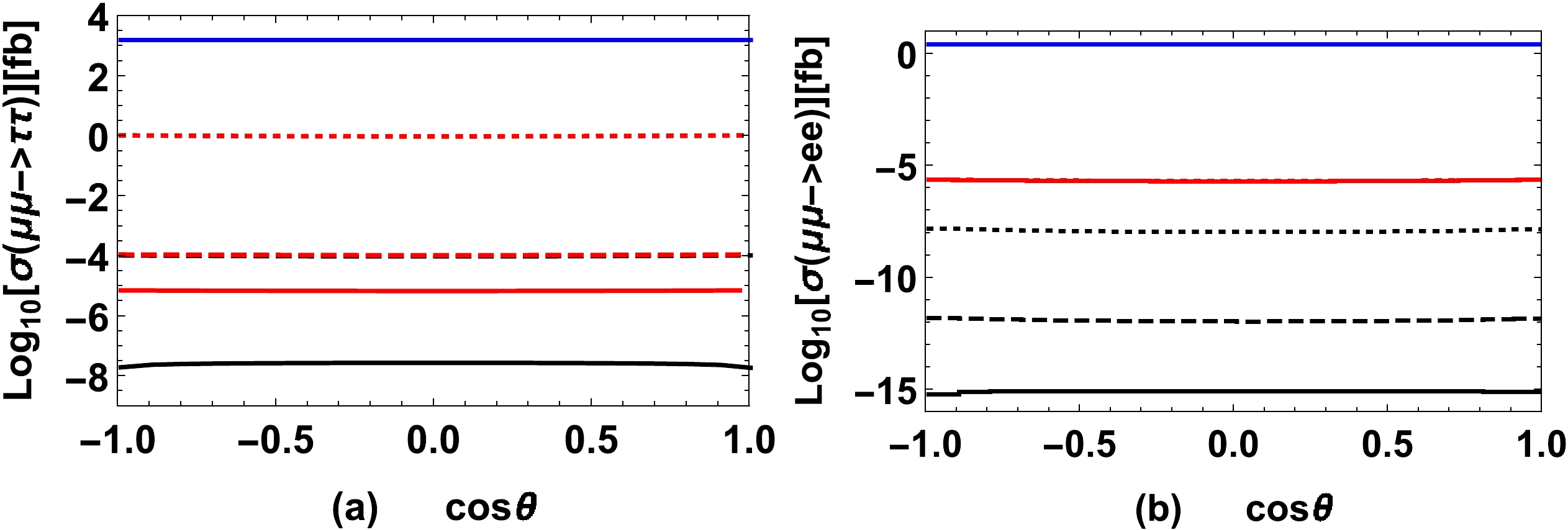

Figure 7.  (color online) Angle distributions of the process $ \mu^\pm \mu^\pm \rightarrow \tau^\pm \tau^\pm $ for $ M_{N_1}=1\;{\rm TeV} $, $ M_{N_2}=2\;{\rm TeV} $, $ M_{N_3}=3\;{\rm TeV} $, $ S_e^2=10^{-5} $, $ S_\tau^2=10^{-2} $, and $ \sqrt s=5\;{\rm TeV} $. $ l=\tau $in (a), and$ l=e $ in (b). The solid, dashed, and dotted curves denote the results with $ S_\mu^2=10^{-6},\;10^{-4},\;10^{-2} $, respectively. The black curves denote the results for TI-NP, the red curves denote the results for TII-NP with $ M_{W_2}=5\;{\rm TeV} $, and the blue curves denote results for TIII-NP with $ M_{W_2}=5\;{\rm TeV} $, $ M_{\Delta^{\pm\pm}}=3\; $TeV, $ Y_{ee}=0.04 $, $ Y_{\mu\mu}=1 $, and$ Y_{\tau\tau}=1 $.

In this subsection, we compute the LNV di-boson processes $ \mu^\pm\mu^\pm\to W^\pm_{i}W^\pm_{j}, (i,j=1,2) $ for TI-NP, TII-NP, and TIII-NP and present the numerical results properly. For the collider search of $ \mu^-\mu^-\to W^-W^- $ (the case of $ \mu^+\mu^+\to W^+W^+ $ collisions is similar), the different decay channels of the final W bosons correspond to different SM background processes. For the pure leptonic channel $ \mu^-\mu^-+E /_T $ and $ \mu^-e^-+E /_T $, where $ E /_T $ denotes the missing energy carried by neutrinos, we compute the SM background processes $ \mu^-\mu^- \rightarrow W^- \mu^-\nu_\mu $ and $ \mu^-\mu^- \rightarrow Z \mu^-\mu^- $ in terms of MadGraph5 [79], and the results at $ \sqrt s=15\;{\rm TeV} $ are as large as

This indicates that they may make significant backgrounds when the pure leptonic channels $ \mu^-\mu^-+E /_T $, $ \mu^-e^-+E /_T $ are considered when observing the LNV processes, and the signals for the LNV processes are very difficult to be picked up from the backgrounds [38]. However, a technique to avoid the problem consists of ignoring all the events in which the decays $ W^-\to \mu^- \bar{\nu}_\mu $ and/or $ W^-\to \tau^- \bar{\nu}_\tau $ with $ \tau^- \to \mu^-\nu_\tau\bar{\nu}_\mu $ are involved, and taking into account only the events in which the $ W^- $ bosons decay either to $ e \bar{\nu}_e $ or $ \tau \bar\nu_\tau $ (except the τ lepton decay $ \tau^-\to \mu^-\nu_\tau \bar{\nu}_\mu $) or quarks ($ q\bar{q'} $). In this way, although the efficiency of identifying W-boson(s) in the final states of the LNV processes will be lost to some extent, the accuracy for identifying the LNV processes will be ensured. Therefore, we will not be concerned with this type of possible SM backgrounds for the LNV anymore. As analyzed in Ref. [38] (which focuses on same-sign electron colliders, with a case of same-sign muon colliders similar to that considered in this work), the dominant SM background process is $ \mu^-\mu^-\rightarrow W^-W^-\nu_\mu\nu_\mu $ for the pure leptonic channel $ e^-e^-+E /_T $. The W bosons in the final state have effective missing energies and momenta due to the involving neutrinos in the final state, which indicates that the background process can be highly suppressed by cutting the invariant-mass of the two outgoing electrons. In addition, it is concluded in Ref. [38] that the semi-leptonic channel $ e^-+j_W+E /_T $ and the pure hadronic channel $ 2j_W $ also have great potential to observe the signal processes.

We stated in Sec. III that the cross section of $ \mu^\pm\mu^\pm\rightarrow W_1^\pm W_1^\pm $ for TII-NP is similar to that of $ \mu^\pm\mu^\pm\rightarrow W_L^\pm W_L^\pm $ for TI-NP, and the cross section of $ \mu^\pm\mu^\pm\rightarrow W_1^\pm W_2^\pm $ for TIII-NP is similar to that of $ \mu^\pm\mu^\pm\rightarrow W_1^\pm W_2^\pm $ for TII-NP. Therefore, for simplicity and avoiding repetition, the results about $ \mu^\pm\mu^\pm\rightarrow W_1^\pm W_1^\pm $ for TII-NP and about $ \mu^\pm\mu^\pm\rightarrow W_1^\pm W_2^\pm $ for TIII-NP will not be presented here.

The results on the cross sections $\sigma(\mu^\pm \mu^\pm \rightarrow W_i^\pm W_j^\pm), \, (i,j=1,2)$ versus $ \sqrt s $ are presented in Fig. 8 for $ M_{N_2}=2.0\;{\rm TeV} $, $ S_\mu^2=10^{-4} $, where the solid, dashed, and dotted curves denote the results for the processes when $ W_iW_j=W_1W_1 $, $ W_1W_2 $, and $ W_2W_2 $ respectively. Figure 8 (a) shows those results with $ M_{\Delta_L^{\pm\pm}}=10.0\;{\rm TeV} $ and $ M_{\Delta_R^{\pm\pm}}=11.0\;{\rm TeV} $ for TIII-NP. Figure 8(b) shows the results with $ M_{\Delta_L^{\pm\pm}}=5.0\;{\rm TeV} $ and $ M_{\Delta_R^{\pm\pm}}=15.0\;{\rm TeV} $ for TIII-NP. The black curve denotes the results for TI-NP, the red curves denote the results for TII-NP with $ M_{W_2}=5.0\; $ TeV, and the blue curves denote the results for TIII-NP with $ M_{W_2}=5.0\; $ TeV and $ Y_{\mu\mu}=1.0 $.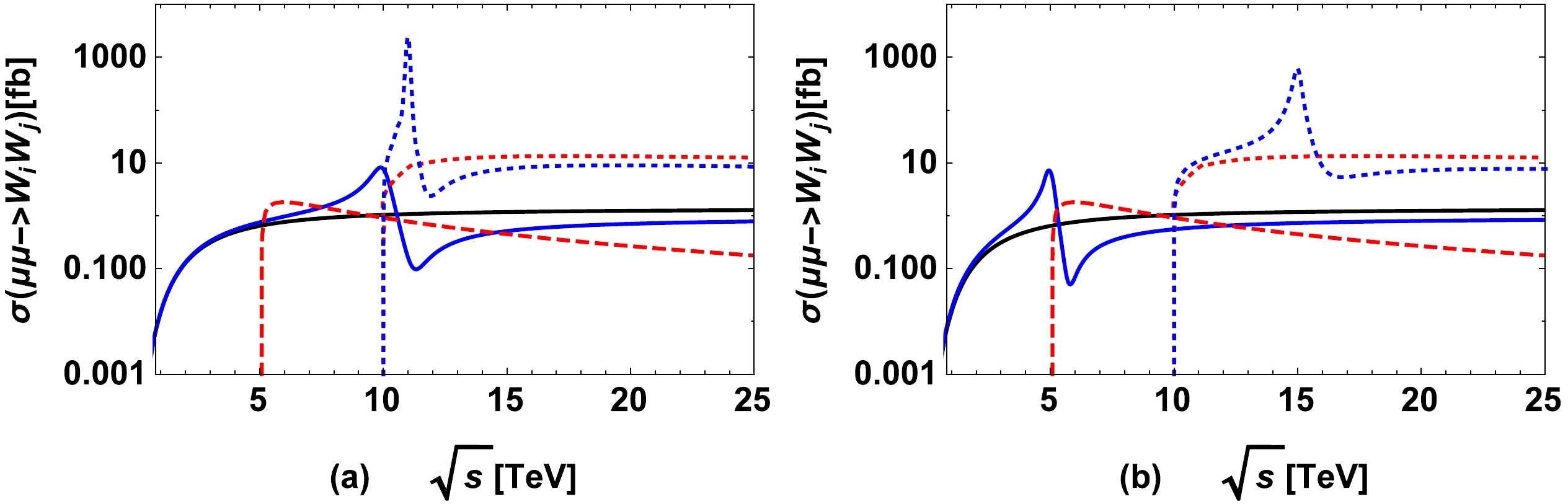

Figure 8.  (color online) $ \sigma(\mu^\pm \mu^\pm \rightarrow W_i^\pm W_j^\pm) $ versus $ \sqrt s $ with $ M_{N_2}=2.0\;{\rm TeV} $, $ S_\mu^2=10^{-4} $, where the solid, dashed, and dotted curves denote the results for the processes when $ W_iW_j=W_1W_1 $, $ W_1W_2 $, $ W_2W_2 $, respectively. In (a), those results are presented with $ M_{\Delta_L^{\pm\pm}}=10.0\;{\rm TeV} $ and $ M_{\Delta_R^{\pm\pm}}=11.0\;{\rm TeV} $ for TIII-NP. In (b), the results are presented with $ M_{\Delta_L^{\pm\pm}}=5.0\;{\rm TeV} $ and $ M_{\Delta_R^{\pm\pm}}=15.0\;{\rm TeV} $ for TIII-NP. The black curves denote the results for TI-NP, the red curves denote the results for TII-NP with $ M_{W_2}=5.0\; $TeV, and the blue curves denote the results for TIII-NP with $ M_{W_2}=5.0\; $TeV and $ Y_{\mu\mu}=1.0 $.

In Fig. 8 the blue dotted curve and the red dotted curve merge together at $ \sqrt s \simeq 10.0\; $ TeV because the process $ \mu^\pm \mu^\pm \rightarrow W_2^\pm W_2^\pm $ starts from $ \sqrt s=10.0\; $ TeV when $ M_{W_2}=5.0\; $ TeV. The enhancement that appears as a hill on the blue curve for $ \sigma(\mu^\pm \mu^\pm \rightarrow W_1^\pm W_1^\pm) $ or $ \sigma(\mu^\pm \mu^\pm \rightarrow W_2^\pm W_2^\pm) $ is the resonance signal due to the $ s- $channel $ \Delta_L^{\pm\pm} $ or $ \Delta_R^{\pm\pm} $, and it corresponds explicitly to the blue solid or blue dotted curves, respectively. In the figure, one can observe the resonance signal caused by $ \Delta_L^{\pm\pm} $ or $ \Delta_R^{\pm\pm} $, i.e., the resonance peak that appears in the process $ \mu^\pm \mu^\pm \rightarrow W_1^\pm W_1^\pm $ or in the process $ \mu^\pm \mu^\pm \rightarrow W_2^\pm W_2^\pm $ at $ \mu^\pm\mu^\pm $ colliders. The observed resonance enhancement appears in $ \mu^\pm \mu^\pm \rightarrow W_1^\pm W_1^\pm $ when the $ s- $channel $ \Delta_L^{\pm\pm} $ plays roles, and the observed resonance enhancement appears in $ \mu^\pm \mu^\pm \rightarrow W_2^\pm W_2^\pm $ when the $ s- $channel $ \Delta_R^{\pm\pm} $ plays roles. In addition, in Fig. 8, a "valley" is observed on the blue solid or blue dotted curve owing to the interference effect between the contributions from Majorana neutral leptons and those from the doubly charged Higgs.

To observe the interference effects indicated by the "hill-valley" structure for TIII-NP in the blue curves in Fig. 8 (a) and Fig. 8 (b) more precisely, we plot $ \sigma(\mu^\pm \mu^\pm \rightarrow W_i^\pm W_i^\pm), (i=1,2) $ versus $ \sqrt s $ in Fig. 9. In (a), $ i=1 $, and in (b), $ i=2 $. The solid, dashed, and dotted curves in the figures denote the results with $ M_{N_2}=1.0,\;2.0,\;3.0\;{\rm TeV} $, respectively. In Fig. 9 (a) the black curves denote the results for TI-NP, the red curves in Fig. 9 (b) denote the results for TII-NP with $ M_{W_2}=5.0\;{\rm TeV} $, and the blue curves in both figures denote the results for TIII-NP with $ M_{W_2}=5.0\;{\rm TeV} $, $ Y_{\mu\mu}=1.0 $, $ M_{\Delta_L^{\pm\pm}}=10.0\;{\rm TeV} $, and $ M_{\Delta_R^{\pm\pm}}=11.0\;{\rm TeV} $. The interference effects between the contributions from doubly charged Higgs and those from the Majorana neutral leptons can be observed clearly (the blue curves) in Fig. 9, and both $ \sigma(\mu^\pm \mu^\pm \rightarrow W_1^\pm W_1^\pm) $ and $ \sigma(\mu^\pm \mu^\pm \rightarrow W_2^\pm W_2^\pm) $ increase with increasing $ M_{N_2} $. The heights of the peaks on the three blue curves in Fig. 9 (a) are similar because the contributions to $ \sigma(\mu^\pm \mu^\pm \rightarrow W_1^\pm W_1^\pm) $ are dominated by $ \Delta_L^{\pm\pm} $ contributions at the resonance, and varying $ M_{N_2} $ does not affect the heights of the resonance peaks at all. However, Fig. 9 (b) shows that the heights of the peaks of the three blue curves vary with $ M_{N_2} $ because $ M_{N_2} $ is related to the Yukawa coupling $ \Delta_R^{\pm\pm} \mu^{\mp}\mu^{\mp} $ and the resonance heights are dominated by the Yukawa coupling.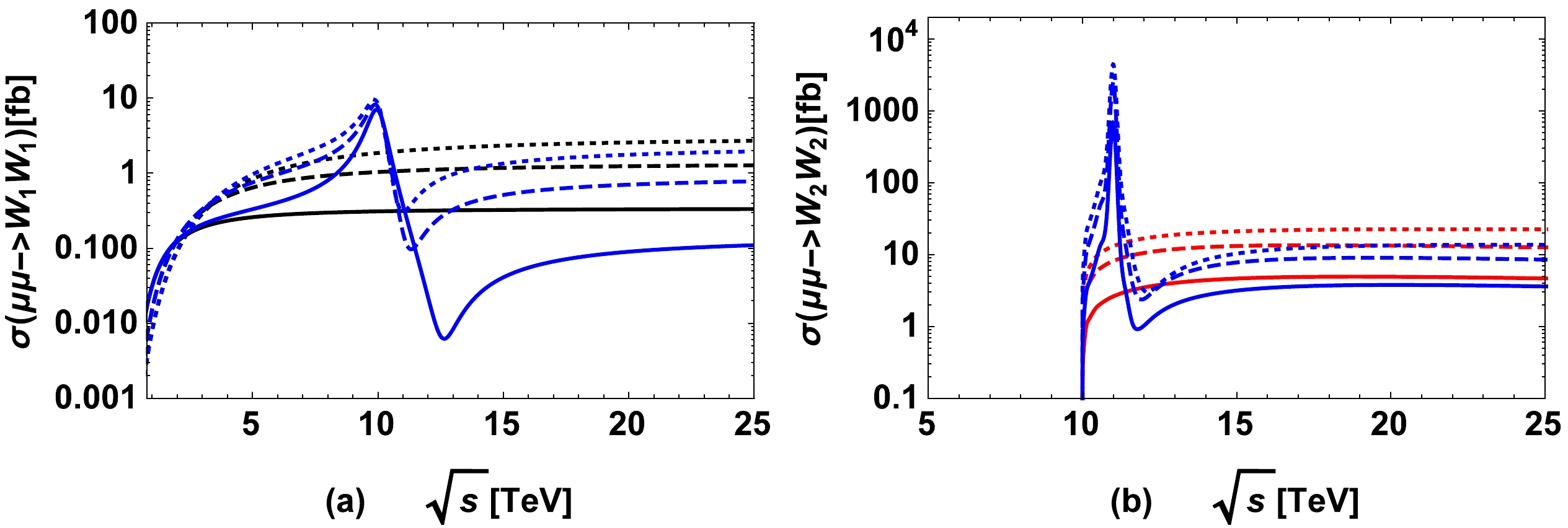

Figure 9.  (color online) $ \sigma(\mu^\pm \mu^\pm \rightarrow W_i^\pm W_j^\pm) $ versus $ \sqrt s $ with $ S_\mu^2=10^{-4} $. In (a), $ W_iW_j=W_1W_1 $, and in (b), $ W_iW_j=W_2W_2 $. The solid, dashed, and dotted curves in the figures denote the results for $ M_{N_2}=1.0,\;2.0,\;3.0\;{\rm TeV} $, respectively. The black curves denote the results for TI-NP, and the red curves denote the results for TII-NP with $ M_{W_2}=5.0\;{\rm TeV} $. The blue curves denote the results for TIII-NP with $ M_{W_2}=5.0\;{\rm TeV} $, $ Y_{\mu\mu}=1.0 $, $ M_{\Delta_L^{\pm\pm}}=10.0\;{\rm TeV} $, and $ M_{\Delta_R^{\pm\pm}}=11.0\;{\rm TeV} $.

To explore and see the effects of $ S_\mu^2 $ on the cross sections $ \sigma(\mu^\pm \mu^\pm \rightarrow W_i^\pm W_j^\pm) $, we set $ M_{N_2}=2.0\;{\rm TeV} $ and $ \sqrt s=15.0\; $ TeV, and the other relevant parameters are the same as those in Fig. 9. We plot $ \sigma(\mu^\pm \mu^\pm \rightarrow W_i^\pm W_j^\pm) $ versus $ S_\mu^2 $ in Fig. 10. The black solid curve denotes the result of $ W_iW_j=W_1W_1 $ for TI-NP. The red dashed and red dotted curves denote the results of $ W_iW_j=W_1W_2 $ and $ W_iW_j=W_2W_2 $, respectively, for TII-NP with $ M_{W_2}=5.0\; $ TeV. The blue solid and blue dotted curves denote the results of $ W_iW_j=W_1W_1 $ and $ W_iW_j=W_2W_2 $, respectively, for TIII-NP with $ M_{W_2}=5.0\; $ TeV, $ Y_{\mu\mu}=1.0 $, $ M_{\Delta_L^{\pm\pm}}= $ 10.0 TeV, and $ M_{\Delta_R^{\pm\pm}}=11.0\; $ TeV. The dotted curves in Fig. 10 indicate that $ \sigma(\mu^\pm \mu^\pm \rightarrow W_2^\pm W_2^\pm) $ is not sensitive to $ S_\mu^2 $, and this fact can be read out from Eq. (33). The results described by the black solid curve and the red dashed curve show that $ \sigma(\mu^\pm \mu^\pm \rightarrow W_1^\pm W_1^\pm) $ for TI-NP, TII-NP and $ \sigma(\mu^\pm \mu^\pm \rightarrow W_1^\pm W_2^\pm) $ for TII-NP, TIII-NP increase with increasing $ S_\mu^2 $. As shown by the blue solid curves in the figures, $ \sigma(\mu^\pm \mu^\pm \rightarrow W_1^\pm W_1^\pm) $ for TIII-NP decreases with the increase in $ S_\mu^2 $ first and then increases with the increase in $ S_\mu^2 $. This is due to the fact that the contributions to the process $ \mu^\pm \mu^\pm \to W_1^\pm W_1^\pm $ for TIII-NP are dominated by the doubly charged Higgs when $ S_\mu^2 $ is small ($ S_\mu^2\lesssim 10^{-5} $), whereas the interference effects of the contributions from Majorana neutral leptons and from the doubly charged Higgs become important when $ S_\mu^2\approx 10^{-4} $ (the interference effects can be observed more clearly in Fig. 9), and the Majorana neutral lepton contributions play dominant roles when $ S_\mu^2 $ is sufficiently large ($ S_\mu^2\gtrsim 10^{-3} $).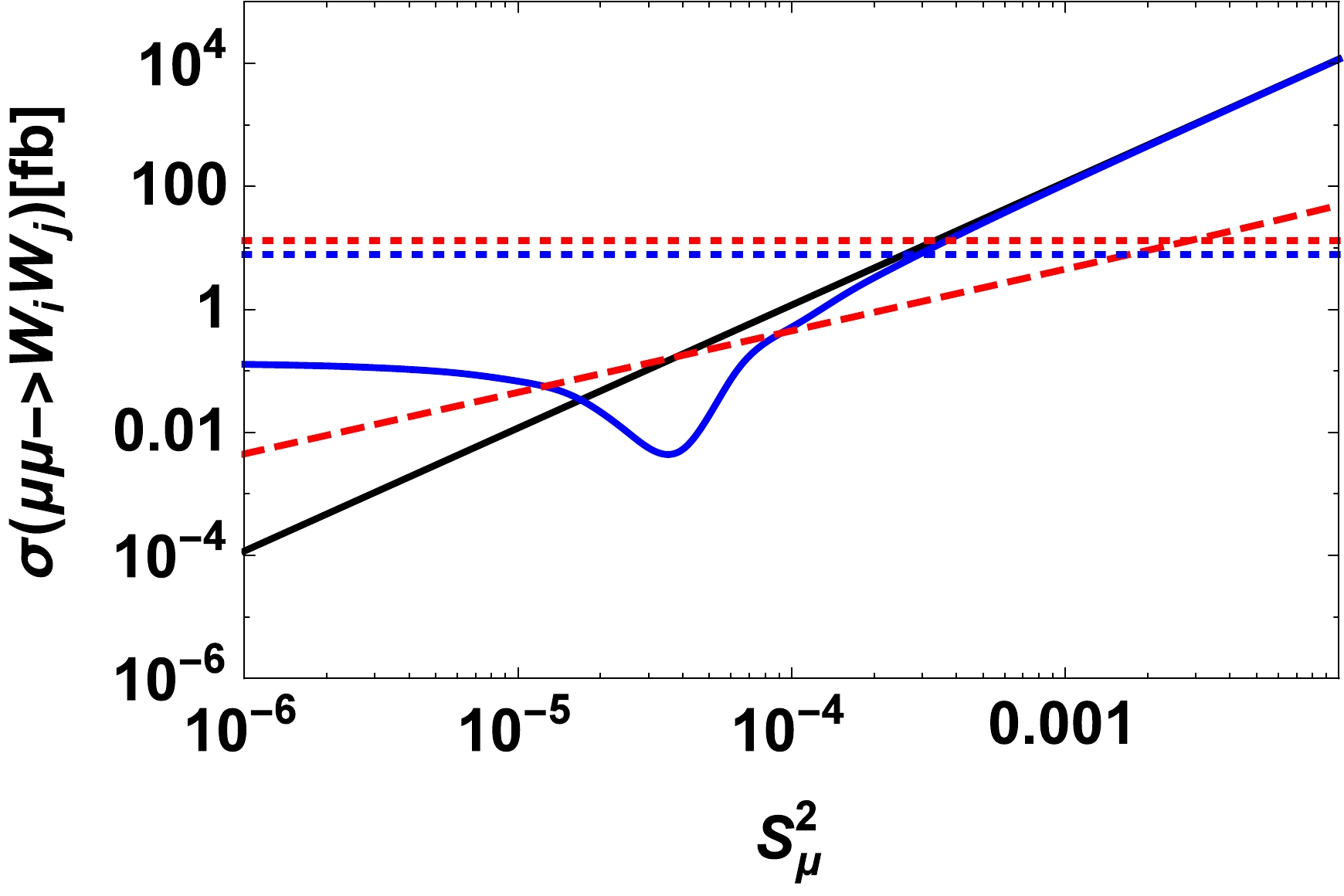

Figure 10.  (color online) $ \sigma(\mu^\pm \mu^\pm \rightarrow W_i^\pm W_j^\pm) $ versus $ S_\mu^2 $ with $ M_{N_2}=2.0\;{\rm TeV} $, $ \sqrt s=15.0\; $TeV (the other relevant parameters are the same as those in Fig. 9). The black solid curve denotes the result of $ W_iW_j=W_1W_1 $ for TI-NP. The red dashed and red dotted curves denote the results of $ W_iW_j=W_1W_2 $ and $ W_iW_j=W_2W_2 $, respectively, for TII-NP with $ M_{W_2}=5.0\; $TeV. The blue solid and blue dotted curves denote the results of $ W_iW_j=W_1W_1 $ and $ W_iW_j=W_2W_2 $, respectively, for TIII-NP with $ M_{W_2}=5.0\; $TeV, $ Y_{\mu\mu}=1.0 $, $ M_{\Delta_L^{\pm\pm}}=10.0\; $TeV, and $ M_{\Delta_R^{\pm\pm}}=11.0\; $TeV.

It is pointed in Ref. [80] that a high energy $ \mu^+\mu^- $ collider running at the collision energy $ \sqrt s\simeq 10\;{\rm TeV} $ can probe $ S_\mu^2 $ down to the region $ \mathcal{O} (10^{-7}) \sim \mathcal{O}(10^{-4}) $ if an integrated luminosity of $ 10^4\;{\rm fb}^{-1} $ is accumulated. Based on same-sign high energy muon colliders with a collision energy such as $ \sqrt s\simeq 15\;{\rm TeV} $, the solid black curve in Fig. 10 shows that the total cross section of the LNV process $ \mu^-\mu^-\rightarrow W_1^- W_1^- $ may reach up-to approximately $ 0.01\;{\rm fb} $ by the prediction of TI-NP with $ S_\mu^2\approx 10^{-5} $. Note from the blue and red curves in Fig. 10 that the cross sections of the LNV processes $ \mu^\pm\mu^\pm\rightarrow W_1^\pm W_1^\pm $ predicted by TII-NP and TIII-NP are larger than that predicted by TI-NP when $ S_\mu^2 < 10^{-4} $; hence, the LNV processes predicted by TII-NP and TIII-NP at a high energy $ \mu^\pm\mu^\pm $ collider have much greater opportunities to be observed. The observation of these processes must offer unambiguous evidences of NP, which is a totally different way to fix the parameter $ S_\mu^2 $ from that at the high energy $ \mu^+\mu^- $ colliders [80]. Moreover, same-sign muon colliders have very special advantages in observing the doubly charged Higgs and setting constraints on the couplings of doubly charged Higgs with charged leptons. In particular, from the facts mentioned here, the complementarity of high energy same-sign muon colliders with high energy $ \mu^+\mu^- $ colliders can be concluded very well.

Taking $ M_{N_2}=2\;{\rm TeV} $, $ S_\mu^2=10^{-4} $, we plot the angle distributions of $ \mu^\pm \mu^\pm \rightarrow W_i^\pm W_j^\pm $ in Fig. 11. Figure 11 (a) shows that of $ W_iW_j=W_1W_1 $ with $ \sqrt s=5\;{\rm TeV} $, where the black curve denotes the results for TI-NP, the blue curves denote the results for TIII-NP with $ M_{W_2}=5\;{\rm TeV} $, $ Y_{\mu\mu}=1 $. The blue solid, blue dashed, and blue dotted curves denote the results with $ M_{\Delta^{\pm\pm}_L}=M_{\Delta^{\pm\pm}_R}=3,\;5,\;7\; $ TeV, respectively. Figure 11 (b) shows that of $ W_iW_j=W_1W_2 $ with $ \sqrt s=7\;{\rm TeV} $, where the red curve denotes the results obtained for TII-NP. Figure 11 (c) presents that of $ W_iW_j=W_2W_2 $ with $ \sqrt s=12\;{\rm TeV} $, where the red curve denotes the results for TII-NP, the blue curves denote the results for TIII-NP with $ Y_{\mu\mu}=1 $, and the blue solid, blue dashed, and blue dotted curves denote the results for $ M_{\Delta^{\pm\pm}_L}=M_{\Delta^{\pm\pm}_R}=7,\;12,\;15\; $ TeV respectively.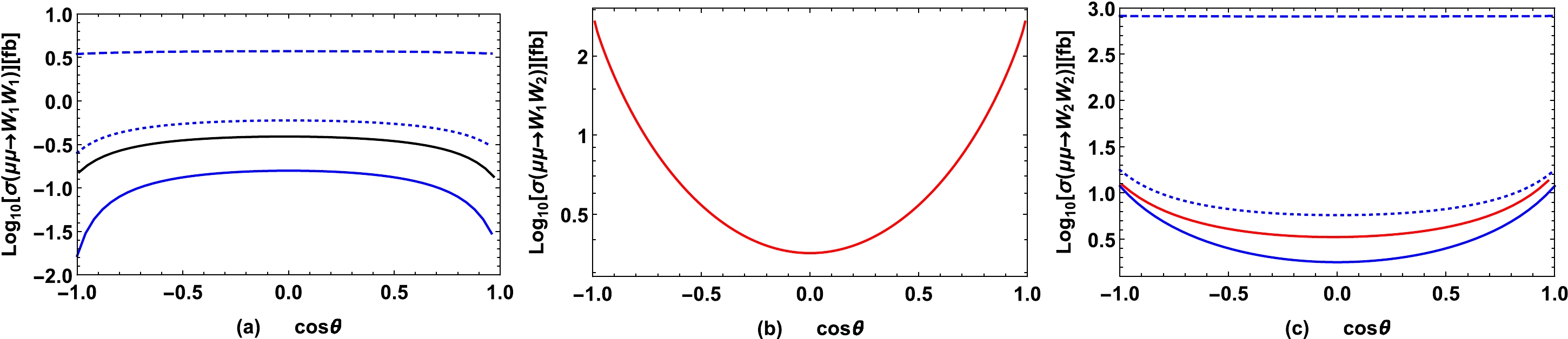

Figure 11.  (color online) Taking $ M_{N_2}=2\;{\rm TeV} $ and $ S_\mu^2=10^{-4} $, (a) angle distributions of $ \mu^\pm \mu^\pm \rightarrow W_1^\pm W_1^\pm $ for $ \sqrt s=5\;{\rm TeV} $, where the black curve denotes the results for TI-NP, the blue curves denote the results for TIII-NP with $ M_{W_2}=5\;{\rm TeV} $ and $ Y_{\mu\mu}=1 $, and the blue solid, blue dashed, and blue dotted curves denote the results for $ M_{\Delta^{\pm\pm}_L}=M_{\Delta^{\pm\pm}_R}=3,\;5,\;7\; $TeV, respectively; (b) angle distributions of $ \mu^\pm \mu^\pm \rightarrow W_1^\pm W_2^\pm $ for $ \sqrt s=7\; $TeV, where the red curve denotes the results for TII-NP; (c) angle distributions of $ \mu^\pm \mu^\pm \rightarrow W_2^\pm W_2^\pm $ for $ \sqrt s=12\; $TeV, where the red curve denotes the results for TII-NP, the blue curves denote the results for TIII-NP with $ Y_{\mu\mu}=1 $, and the blue solid, blue dashed, and blue dotted curves denote the results for $ M_{\Delta^{\pm\pm}_L}=M_{\Delta^{\pm\pm}_R}=7,\;12,\;15\; $TeV, respectively.

As shown in the figures, the angular distributions of the process $ \mu^\pm \mu^\pm \rightarrow W_i^\pm W_i^\pm\;(i=1,2) $ predicted by TIII-NP are flat for $ \sqrt s\approx M_{\Delta^{\pm\pm}_L}=M_{\Delta^{\pm\pm}_R} $ because the contributions to the processes are dominated by the s-channel doubly charged Higgs in this case. The black solid, blue solid, and blue dotted curves in Fig. 11 (a) show that $ \sigma(\mu\mu\rightarrow W_1W_1) $ takes the maximum value at $ \cos\theta=0 $, and the contributions to the process are dominated by Majorana neutral leptons in these three cases. Figures 11 (b) and (c) show that $ \sigma(\mu\mu\rightarrow W_1W_2) $ predicted by TII-NP, TIII-NP and $ \sigma(\mu\mu\rightarrow W_2W_2) $ predicted by TII-NP take the minimum values at $ \cos\theta=0 $. The angular distributions of the process $ \mu^\pm \mu^\pm \rightarrow W_2^\pm W_2^\pm $ predicted by TIII-NP are flat when the contributions are dominated by doubly charged Higgs, and $ \sigma(\mu\mu\rightarrow W_2W_2) $ takes the minimum value at $ \cos\theta=0 $ when the contributions are dominated by Majorana neutral leptons.

It will be feasible to build a high energy $ \mu^+\mu^- $ collider in the future once progresses on the relevant techniques are achieved. Then, building a very high energy same-sign $ \mu^\pm \mu^\pm $ collider should have no additional serious technical problems. Therefore, it is crucial to investigate important physics phenomena, such as lepton di-flavor violation (LFV) processes $ \mu^\pm \mu^\pm \rightarrow e^\pm e^\pm $ and $ \mu^\pm \mu^\pm \rightarrow \tau^\pm \tau^\pm $ and lepton di-number violation (LNV) processes $ \mu^\pm \mu^\pm \rightarrow W_i^\pm W_j^\pm $ ($ i,\;j=1,\;2 $), at very high energy $ \mu^\pm \mu^\pm $ colliders. All of these processes are forbidden in the SM, and the observation of these processes is sensitive to the nature of the heavy neutral leptons and neutrinos, for example, the LFV and LNV physics at TeV energy scale and the doubly charged Higgs in certain new physics (NP) models. In this regard, we have performed quantitative evaluations of the NP contributions to these processes and explored their essential characteristics by categorizing the involved NP factors into three types. Taking into account the constraints imposed by existing experiments, we have computed and appropriately presented the numerical results in figures. This section provides brief discussions on the obtained results and summarizes the significance of observing LFV di-lepton and LNV di-boson processes at TeV-scale $ \mu^\pm \mu^\pm $ colliders.

For the LFV di-lepton processes, Figs. 4−6 clearly show that the predicted $ \sigma(\mu^\pm \mu^\pm \rightarrow \tau^\pm \tau^\pm) $ and $ \sigma(\mu^\pm \mu^\pm \rightarrow e^\pm e^\pm) $ can reach $ 10\;{\rm fb} $ and $ 10^{-6}\;{\rm fb} $, respectively, for TI-NP and TII-NP. This indicates that the process $ \mu^\pm \mu^\pm \rightarrow \tau^\pm \tau^\pm $ has great opportunities to be observed at the high energy $ \mu^\pm \mu^\pm $ colliders, whereas the process $ \mu^\pm \mu^\pm \rightarrow e^\pm e^\pm $ is comparatively harder to be observed at such $ \mu^\pm \mu^\pm $ colliders. For TIII-NP, the contributions to the LFV di-lepton processes are dominated by doubly charged Higgs in most cases, and the results are much larger than those for TI-NP and TII-NP. Both the $ \mu^\pm \mu^\pm \rightarrow \tau^\pm \tau^\pm $ and $ \mu^\pm \mu^\pm \rightarrow e^\pm e^\pm $ processes predicted by TIII-NP have great opportunities to be observed at high energy $ \mu^\pm \mu^\pm $ colliders. Furthermore, Fig. 5 clearly demonstrates the resonance enhancements caused by the two $ s- $channel doubly charged Higgs for TIII-NP. This implies that the LFV processes $ \mu^\pm\mu^\pm\rightarrow \tau^\pm \tau^\pm $ and $ \mu^\pm\mu^\pm\rightarrow e^\pm e^\pm $ serve as favorable channels for observing the two doubly charged Higgs at high energy $ \mu^\pm \mu^\pm $ colliders. The angular distributions of $ \mu^\pm \mu^\pm \rightarrow \tau^\pm \tau^\pm $ and $ \mu^\pm \mu^\pm \rightarrow e^\pm e^\pm $ predicted for TI-NP, TII-NP, and TIII-NP are flat, which indicates that the di-lepton processes predicted in all these three types of NP are insensitive to the angular cuts (Fig. 7).

For the LNV di-boson processes, the results for $ \sigma(\mu^\pm\mu^\pm\rightarrow W_1^\pm W_1^\pm) $ for TII-NP are similar to those for $ \sigma(\mu^\pm\mu^\pm\rightarrow W_L^\pm W_L^\pm) $ for TI-NP, and the results for $ \sigma(\mu^\pm\mu^\pm\rightarrow W_1^\pm W_2^\pm) $ for TIII-NP are similar to those for $ \sigma(\mu^\pm\mu^\pm\rightarrow W_1^\pm W_2^\pm) $ for TII-NP. Figures 8−10 clearly demonstrate that $ \sigma(\mu^\pm \mu^\pm \rightarrow W_1^\pm W_1^\pm) $ predicted by TI-NP and TII-NP can reach a large value approximately as $ 10^4\;{\rm fb} $ when $ \sqrt s=15\;{\rm TeV} $, and the cross-section $ \sigma(\mu^\pm \mu^\pm \rightarrow W_1^\pm W_2^\pm) $ predicted by TII-NP and TIII-NP can reach approximately $ 100\;{\rm fb} $ when $ \sqrt s=15\;{\rm TeV} $. The resonance enhancements in $ \sigma(\mu^\pm \mu^\pm \rightarrow W_1^\pm W_1^\pm) $ and $ \sigma(\mu^\pm \mu^\pm \rightarrow W_2^\pm W_2^\pm) $ are due to the contributions from doubly charged Higgs for TIII-NP. Thus, observing the processes $ \mu^\pm \mu^\pm \rightarrow W_1^\pm W_1^\pm $ and $ \mu^\pm \mu^\pm \rightarrow W_2^\pm W_2^\pm $ at very high energy $ \mu^\pm\mu^\pm $ colliders represents a valuable approach to observe the relevant signals originated from either $ \Delta_L^{\pm\pm} $ or $ \Delta_R^{\pm\pm} $. Measuring the total decay widths of $ \Delta_L^{\pm\pm} $ and $ \Delta_R^{\pm\pm} $ for TIII-NP via observing the LNV di-boson processes is also an important topic for the high energy $ \mu^\pm \mu^\pm $ colliders. The results of angle distributions (Fig. 11) show that $ {\rm d}\sigma(\mu\mu\rightarrow W_1W_1)/{\rm d}\cos\theta $ predicted for TI-NP, TII-NP takes the maximum value at $ \cos\theta=0 $. For TIII-NP, the angular distributions of the process $ \mu^\pm \mu^\pm \rightarrow W_1^\pm W_1^\pm $ are flat when the contributions to $ \mu^\pm \mu^\pm \rightarrow W_1^\pm W_1^\pm $ are dominated by doubly charged Higgs, and $ \sigma(\mu\mu\rightarrow W_1W_1) $ takes the maximum value at $ \cos\theta=0 $ when the contributions are dominated by Majorana neutral leptons. $ \sigma(\mu\mu\rightarrow W_1W_2) $ predicted for TII-NP and TIII-NP and $ \sigma(\mu\mu\rightarrow W_2W_2) $ predicted for TII-NP take the minimum values at $ \cos\theta=0 $. The angular distributions of the process $ \mu^\pm \mu^\pm \rightarrow W_2^\pm W_2^\pm $ predicted for TIII-NP are flat when the contributions are dominated by doubly charged Higgs, and $ \sigma(\mu\mu\rightarrow W_2W_2) $ takes the minimum value at $ \cos\theta=0 $ when the contributions are dominated by Majorana neutral leptons.

In summary, observing the LFV and LNV processes represents one of the most important physics aspects at high energy $ \mu^\pm\mu^\pm $ colliders. The quantitative investigations presented in this paper lead us to conclude that the LFV process $ \mu^\pm \mu^\pm \rightarrow \tau^\pm \tau^\pm $ predicted by TI-NP, TII-NP, and TIII-NP is highly expected to be observed at very high energy $ \mu^\pm\mu^\pm $ colliders, whereas the process $ \mu^\pm \mu^\pm \rightarrow e^\pm e^\pm $ is expected to be observed only for TIII-NP. Further, all of the LNV di-boson processes predicted by TI-NP, TII-NP, and TIII-NP have great opportunities to be observed at such colliders. Based on the numerical results analyzed in Sec. IV, we can have more insights into the characteristics of the processes due to NP, and achieve the relevant constraints on parameters such as $ M_N $, $ M_{W_2} $, $ Y_{\mu\mu} $, $ M_{\Delta_L^{\pm\pm}} $, and $ M_{\Delta_R^{\pm\pm}} $. It should be emphasized that, at such high energy $ \mu^\pm\mu^\pm $ colliders, there are significant opportunities to observe the NP factors, such as the leptonic Majorana components, right-handed W-bosons, and two doubly charged Higgs and their properties.

Therefore, owing to the support of important physics and absence of serious problems in building high energy same-sign muon colliders, as explored in this paper, we believe that both high energy $ \mu^+\mu^- $ colliders and same-sign $ \mu^\pm\mu^\pm $ colliders will be built in future when techniques such as muon acceleration, muon beam storage in a circular ring, and collision of two counter-propagating muon beams become mature.

The authors (J-L Yang and C-H Chang) would like to thank Prof S-S Bao (SDU) for helpful discussions about MadGraph5.