


 Abstract
 HTML
HTML Reference
 Related
 PDF
PDF


-
The LHCb collaboration found a very narrow peak structure named
$ T^+_{cc} $ in the$ D^0D^0\pi^+ $ invariant mass spectrum in the$ pp \to X + D^0D^0\pi^+ $ process [1]. The mass parameters obtained from a generic constant-width Breit-Wigner fit were listed as$ \delta m_{\rm BW} = -273 \pm 61 \pm 5^{+11}_{-14}\; \mathrm{keV} ,\,\,\, \Gamma_{\rm BW} = 410 \pm 165 \pm 43^{+18}_{-38}\; \mathrm{keV}\,, $

where
$\delta m_{\rm BW}$ defines the mass shift with respect to the$ D^{*+}D^0 $ threshold. Later, it was suggested that$ T^+_{cc} $ could more possibly be an isoscalar state with spin-parity quantum numbers$ J^P = 1^+ $ [2], and in a more complicated model, the pole mass and width were extracted as$ \delta m_{\rm pole} = -360 \pm 40^{+4}_{-0} \; \mathrm{keV}\ ,\,\,\, \Gamma_{\rm pole} = 48\pm 2^{+0}_{-14}\; \mathrm{keV}\,. $

The constituent of
$ T^+_{cc} $ is$ cc\bar{u}\bar{d} $ and there is no annihilated quark pair, similar to$ X_1(2900) $ ($ ud\bar{s}\bar{c} $ ) [3, 4].This experimental observation has stimulated numerous theoretical discussions. First of all, there have been some dynamical lattice QCD simulations about double charmed tetraquarks, although they have not provided a definite conclusion on the existence of the
$ T^+_{cc} $ state [5, 6]. Recently, based on (2+1)-flavor lattice QCD simulations, the$ D^*D $ system was studied more carefully. It was verified that there is a loosely-bound state near the threshold (–10 keV) [7]. Many phenomenological studies have also been conducted. A theoretical prediction indicated that there may exist a$ cc\bar{u}\bar{d} $ tetraquark with$ J^P = 1^+ $ near the$ D^{*+}D^0 $ threshold [8, 9]. In addition, the heavy meson chiral effective field theory (HMChEFT), which considers contact and one pion exchange (OPE) interaction, was used. The preferred conclusion of the analyses is that the$ T^+_{cc} $ state is a molecule of$ D^{*+}D^0 $ and$ D^{*0}D^+ $ [10, 11]. The effect of the triangle diagram singularity was also evaluated with$ D^*D\pi $ interactions. It was found that the contribution is very weak compared with that of the tree diagram, which suggests that$ T^+_{cc} $ is not generated from the triangle singularity [12]. The pole parameters of$ T^+_{cc} $ extracted from a simple K-matrix amplitude were also studied and it was found that$ T^+_{cc} $ may originate from a$ D^{*+}D^0 $ virtual state [13]. The extended chiral Lagrangian with K-matrix unitarity approach was also applied, and it was suggested that vector meson exchanges could play a crucial role in forming the$ T^+_{cc} $ bound state of$ D^*D $ [14].In this work, to determine whether
$ T^+_{cc} $ is just a loosely-bound s-wave molecule of$ D^*D $ or it contains the$ cc\bar{u}\bar{d} $ ingredient, different approaches are used. First, we adopt an approach similar to that of Ref. [14], in which a coupled channel unitarity approach ($ D^{*+}D^0 $ and$ D^{*0}D^+ $ ) with the interaction stemming from the extended hidden local gauge lagrangian was also applied. In Ref. [14], the authors only considered the vector exchanging diagram contributions and there was no fitting of the lineshape data. In this study, more complete interactions, including pseudoscalar, vector exchanges, and$ D^*D $ contact terms, are introduced, and a combined fit of$ DD\pi $ ,$ D\pi $ , and$ DD $ channels is made. It indicates that the ρ vector meson exchange couplings really make non-negligible contributions in generating the$ T^+_{cc} $ resonance compared with the other two interactions. In this scheme, there exists a bound state near the$ D^{*+}D^0 $ threshold, which suggests that$ T^+_{cc} $ may be a$ D^*D $ molecule. Furthermore, the Flatté-like parametrization is also examined. Through a combined fit on three-body and two-body invariant mass spectrum, we find that the result is the same based on the pole counting rule (PCR) and spectral density function sum rule calculation [15−20]: there is only one pole near$ D^*D $ threshold and the corresponding$ \mathcal{Z} \simeq 1 $ . We also attempt to judge the compositeness of$ T^{+}_{cc} $ by comparing its production ($ pp\to T^{+}_{cc} + X $ ) with different theoretical estimations. However, it is difficult to make a clear judgement using this approach.This paper is organized as follows: Sec. I is the introduction, in Sec. II, the K-matrix unitarization approach using an effective Lagrangian in s-wave approximation is introduced and its numerical fit is shown. In Sec. III, other frameworks are employed to analyze the compositeness of
$ T^+_{cc} $ . Finally, in Sec. IV, a brief conclusion on the structure of$ T^+_{cc} $ is drawn. -
We start off from a
$S U(4)$ invariant effective Lagrangian, and then modify the relevant parameters to only preserve the$S U(2)$ symmetry later, as in [21]. Here, we list the relevant coupling terms,$ \begin{aligned}[b] \mathcal{L} =& \mathcal{L}_0 - {\rm i} g\mathrm{Tr}([P,\partial_\mu P]V^\mu)+ {\rm i} g\mathrm{Tr}([V^\nu, \partial_\mu V_\nu]V^\mu)\\ & -\frac{g^2}{2}\mathrm{Tr}([P,V_\mu]^2)+\frac{g^2}{4}\mathrm{Tr}([V_\mu,V_\nu]^2)\ , \end{aligned} $

(1) where
$ \mathcal{L}_0 $ is the free Lagrangian for the pseudoscalar and vector mesons. P and V denote, respectively, the properly normalized pseudoscalar and vector meson matrices$ \begin{array}{*{20}{l}} P = \begin{pmatrix} \dfrac{\eta}{\sqrt{3}}+\dfrac{\eta'}{\sqrt{6}}+\dfrac{\pi^0}{\sqrt{2}}&\pi^+&K^+&\bar{D}^0\\ \pi^-&\dfrac{\eta}{\sqrt{3}}+\dfrac{\eta'}{\sqrt{6}}-\dfrac{\pi^0}{\sqrt{2}}&K^0&D^-\\ K^-&\bar{K}^0&-\dfrac{\eta}{\sqrt{3}}+\sqrt{\dfrac{2}{3}}\eta'&D^-_s\\ D^0&D^+&D^+_s&\eta_c \end{pmatrix}\ , \end{array} $ 
(2) $ \begin{array}{*{20}{l}} V = \begin{pmatrix} \dfrac{\omega}{\sqrt{2}}+\dfrac{\rho^0}{\sqrt{2}}&\rho^+&K^{*+}&\bar{D}^{*0}\\ \rho^-&\dfrac{\omega}{\sqrt{2}}-\dfrac{\rho^0}{\sqrt{2}}&K^{*0}&D^{*-}\\ K^{*-}&\bar{K}^{*0}&\phi&D^{*-}_s\\ D^{*0}&D^{*+}&D^{*+}_s&J/\psi \end{pmatrix}\ . \end{array} $

(3) In the later discussions, all the coupling constants denoted as g in the vertices of the PPV, VVV, and PPVV types in Eqs. (2) and (3) could be different for the vertices of different isospin multiplets, such that only the
$S U(2)$ isospin symmetry is retained. Hereafter, we only consider the vertices relevant to our discussions. We adopt previous theoretical works [18, 21, 22] to estimate these coupling constants because the interaction vertices are similar to theirs with only normalization constant differences, which can be tracked with a careful analysis.From Eq. (1), we can obtain the contact, t, and u channel diagrams of the
$ D^{*+}D^0\to D^{*0}D^+ $ process. We list their amplitudes successively. First, for the contact diagrams in Fig. 1,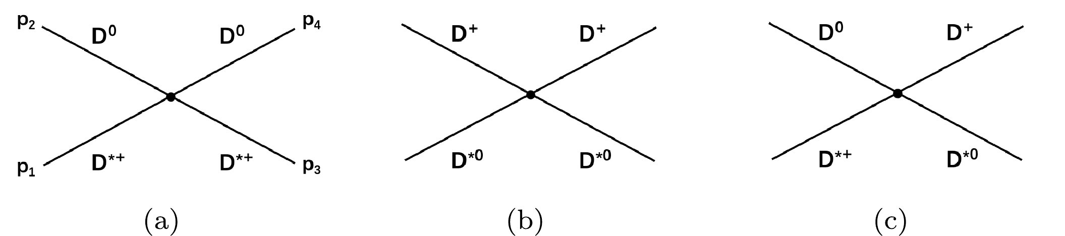
Figure 1. Contact diagrams.
$ \begin{array}{*{20}{l}} {\rm i} M^{c}_{ij} = {\rm i}\, g_{D^*DD^*D}^2, \end{array} $

(4) where
$ i,j = 1,2 $ refer to the$ D^{*+}D^0 $ and$ D^{*0}D^+ $ channels, respectively. The coupling$ g_{D^*DD^*D} $ was estimated when studying$ X(3872) $ [18], that is,$ g (=g_{D^*DD^*D}) \simeq 16 $ 1 .The t channel diagrams include vector meson (
$ J/\psi $ or ρ, ω) exchanges [14], as shown in Fig. 2.2 We also neglect the momentum dependence in the denominator of the propagator near the threshold. Here, the estimates about the coupling constants from the PPV and VVV vertices are as follows: For$ i, j = 1,1 $ or$ 2,2 $ , the coupling constant$ g(= g_{J/\psi D^{(*)}D^{(*)}})\simeq 7.7 $ , and for$ i, j = 1,2 $ or$ 2,1 $ ,$ g(= g_{\rho D^{(*)}D^{(*)}}) \simeq 3.9 $ , which are obtained from the vector meson dominance (VMD) assumption [21]. The t-channel amplitudes are hence written down as follows: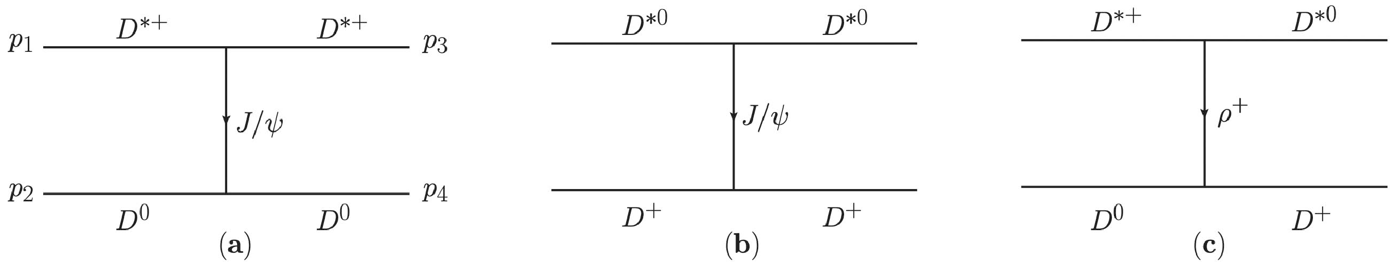
Figure 2. t channel diagrams.
$ \begin{array}{*{20}{l}} {\rm i} M^t_{ij} = {\rm i} D_{ij} (p_1 +p_3)\cdot(p_2 +p_4)\; \epsilon(p_1)\cdot\epsilon^*(p_3), \end{array} $

(5) where
$ \begin{array}{*{20}{l}} D_{ij} = \begin{pmatrix} \dfrac{g^2_{J/\psi D^{(*)}D^{(*)}}}{M^2_{J/\psi}}&\dfrac{g^2_{\rho D^{(*)}D^{(*)}}}{m^2_\rho}\\ \dfrac{g^2_{\rho D^{(*)}D^{(*)}}}{m^2_\rho}&\dfrac{g^2_{J/\psi D^{(*)}D^{(*)}}}{M^2_{J/\psi}}\\ \end{pmatrix}_{ij}. \end{array} $

(6) The third type are u channel diagrams with π exchanges as shown in Fig. 3, and the amplitudes are
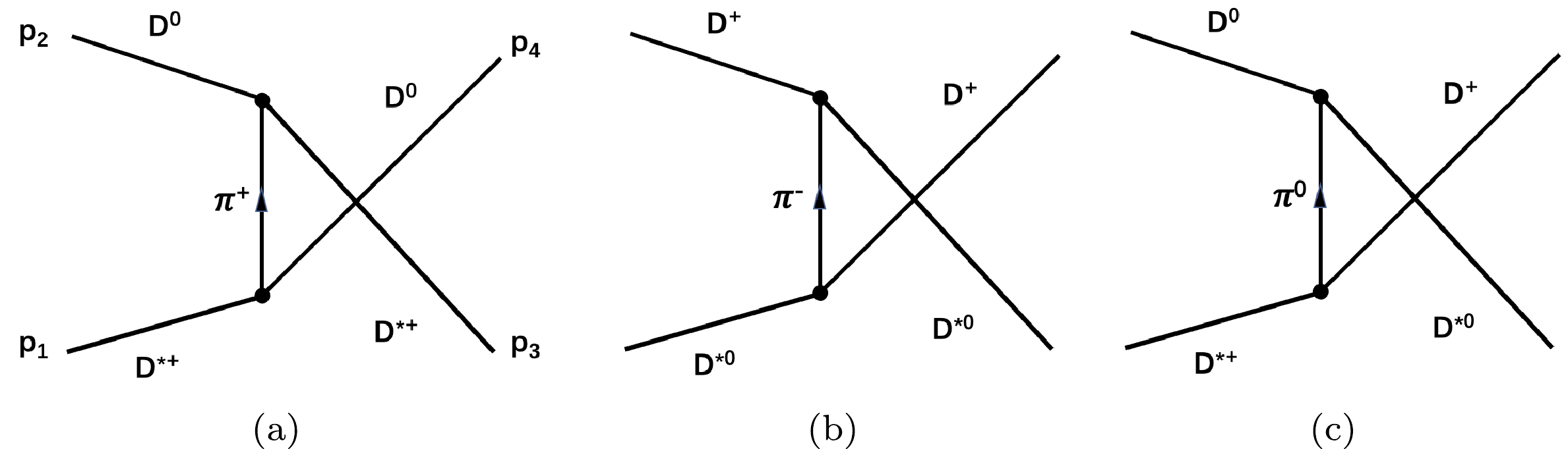
Figure 3. u channel diagrams.
$ {\rm i} M^u_{ij} = {\rm i} E_{ij} g_{\pi DD^*}^2\frac{\epsilon(p_1)\cdot (p_1-2p_4)\; \epsilon^*(p_3)\cdot (p_3-2p_2)}{(p_1-p_4)^2-m_\pi^2}, $

(7) where
$ \begin{array}{*{20}{l}} E_{ij} = \begin{pmatrix} -1&\dfrac{1}{2}\\ \dfrac{1}{2}&-1\\ \end{pmatrix}_{ij}. \end{array} $

(8) The coupling strength
$ g_{\pi DD^*} $ can be restricted by the decay process$ D^{*+} \to D^0 \pi^+ $ , and we take the value$ g(=g_{\pi DD^*}) \simeq 8.4 $ [22]. u-channel diagrams with pseudo-scalar meson$ \eta_c $ exchanges also exist. They are not important at this energy range as it is tested numerically, so we neglect these diagrams. As for the amplitudes corresponding to Fig. 3, the u-channel π exchange is somewhat special because it is possible to exchange one on-shell π meson. After partial wave projection, there exists, in tree level amplitudes, an additional cut in the energy region above the$ D^{*+}D^0 $ threshold. Here, this singularity will affect the unitarity. To remedy this, we adopt the approximate relation$ m_{D^*} = m_{D} + m_{\pi} $ to keep the unitarity threshold away from the singularity, as in Refs. [10, 11]. At last, we obtain the total coupled channel amplitudes$ \begin{array}{*{20}{l}} M_{ij} = M^c_{ij} + M^t_{ij} +M^u_{ij} \ . \end{array} $

(9) Furthermore, with the assumption that the full amplitude is mainly contributed by the s-wave amplitude and the d-wave amplitude can be neglected, we consider the s-wave amplitude, which can be unitarized by the relation
$ \begin{array}{*{20}{l}} {\bf{T}}^{-1} = {\bf{K}}^{-1} - {\bf{g}}(s), \end{array} $

(10) where
$ {\bf{T}} $ is the unitarized s-wave scattering T matrix,$ {\bf{K}} $ is the two-channel s-wave scattering amplitude matrix from$ M_{ij} $ [23], and$ {\bf{g}}(s)\equiv \mathrm{diag}\{g_i(s)\} $ . In our normalization convention$ \begin{aligned}[b]& g_i(s;M_i,m_i) \\=& -16\pi^2 {\rm i}\int \frac{{\rm d}^4q}{(2\pi)^4} \frac{1}{(q^2-M_i^2+ {\rm i}\epsilon)((P-q)^2-m_i^2+ {\rm i}\epsilon)},\,\, (s = P^2) \end{aligned} $

(11) where
$ M_i $ is the vector meson mass and$ m_i $ is the pseudoscalar meson mass in the i-th channel. The expression of$ g_i(s) $ in Eq. (11) is renormalized using the standard$ \overline{\mathrm{MS}} $ scheme, which introduces an explicit renormalization scale (μ) dependence. In our fit, we select the same μ parameter in the two channels.To obtain a finite width for the
$ T_{cc}^+ $ state below the$ D^*D $ threshold, we need to consider the finite width of the$ D^* $ state. This is accomplished by performing a convolution of the$ g_i(s) $ functions with the mass distribution of the$ D^* $ states [24]:$ S\left(s_V;M_V,\Gamma_V\right) \equiv -\frac{1}{\pi} \operatorname{Im}\left\{\dfrac{1}{s_V-M_V^2+ {\rm i} M_V \Gamma_V}\right\} $

(12) such that
$ \tilde{g}_i(s;M_i,m_i)=\mathcal{C} \int_{s_{V \min}}^{s_{V \max}} {\rm d} s_V g_i(s;\sqrt{s_V},m_i) S\left(s_V;M_i,\Gamma_{i}\right) , $

(13) where
$ \mathcal{C} $ is a normalization factor. The main contribution to this integration is from the region around the unstable mass$ s_V\sim M_V^2 $ , so we can introduce a cutoff$ s_{V \min} $ and$s_{V \max}$ . For example, for$ \tilde{g}_1 $ , it is integrated from$ (m_{D_0}+ m_{\pi^+})^2 $ to$ (m_{D^{*+}}+2\Gamma_{D^{*+}})^2 $ , whereas for$ \tilde{g}_2 $ , it is integrated from$ (m_{D_0}+m_{\pi^0})^2 $ to$ (m_{D^{*0}}+2\Gamma_{D^{*0}})^2 $ . Here, in principle,$ \Gamma_i $ is s-dependent as in Ref. [14]. However, we approximate the decay widths as constants because we only focus on a small region near the$ D^{*+}D^0 $ threshold, and we also verified that it makes little difference if the s dependence is included in the numerical calculations. The constant decay widths suggested by PDG [25] read$ \begin{array}{*{20}{l}} \Gamma_{D^{*+}} = 83.4\; \mathrm{keV},\; \; \Gamma_{D^{*0}} = 55.3\; \mathrm{keV}. \end{array} $

(14) To fit the final state three-body invariant mass spectrum of
$ D^0D^0\pi^+ $ in$ pp \to X + D^0D^0\pi^+ $ , the final-state interaction (FSI) [20] between$ D^{*+}D^0 $ and/or$ D^{*0}D^+ $ needs to be considered as above, before contemplating the$ D^{*+}\to D^0+\pi^+ $ decay. The amplitude for the$ D^{*+} D^0 $ final state reads$ \begin{array}{*{20}{l}} \mathcal{F}_{D^{*+} D^{0}}(s)=\alpha_{1}\; T_{11}+\alpha_{2}\; T_{21}\ , \end{array} $

(15) where
$ \alpha_1 $ ,$ \alpha_2 $ are smooth real polynomials parametrizing the amplitude of producing$ D^{*+}D^0 $ and$ D^{*0}D^+ $ , respectively, and as the energy region of interest is very small, we treat them as constant parameters near the thresholds of$ D^{*+}D^0 $ and$ D^{*0}D^+ $ . Finally, the decay of$ T^+_{cc}\to D^0D^0\pi^+ $ can therefore be expressed as in Fig. 4, and the final s-wave scattering amplitude is written as3 
Figure 4. Process of
$ T^+_{cc}\to D^0D^0\pi^+ $ .$ \begin{aligned}[b] t = &\mathcal{F}_{D^{*+}D^0}\left[ \frac{ {\epsilon}\cdot[({p}_1-{p}_2)+\dfrac{m_{\pi^+}^2-m_{D^0}^2}{m_{D^{*+}}^2}({p}_1+{p}_2) ]}{M_{12}^2-m_{D^{*+}}^2+ {\rm i} M_{12}\Gamma_{D^{*+}}(M_{12})}\right.\\ &\left.+\frac{ {\epsilon}\cdot [({p}_3-{p}_2)+\dfrac{m_{\pi^+}^2-m_{D^0}^2}{m_{D^{*+}}^2}({p}_3+{p}_2) ]}{M_{23}^2-m_{D^{*+}}^2+ {\rm i} M_{23}\Gamma_{D^{*+}}(M_{23})} \right]. \end{aligned} $

(16) Here,
$ M_{12} $ and$ M_{23} $ are Dalitz kinematic variables of the final three-body state. The corresponding definition is$ s_{ij}=M_{ij}^2 = (p_i + p_j)^2 $ , and$ {\epsilon}={\epsilon}(P) $ corresponds to the polarization vector of$ T^+_{cc} $ ,$ P=\left(p_{1}+p_{2}+p_{3}\right) $ , and$ P^{2}=s $ . These invariants have the relation$M^2_{12} + M^2_{13} + M^2_{23} = P^2 + p_1^2+ p_2^2+ p_3^2$ . Finally, the decay width of$ T_{cc}^+ $ is given by$ {\rm d}\Gamma(\sqrt{s}) = \frac{\mathcal{N}}{2} \frac{32}{\pi}\frac{1}{s^{3/2}} |t|^2 {\rm d} s_{12} {\rm d} s_{23}. $

(17) The factor
$\dfrac{1}{2}$ in the above equation results from averaging the two integrals of$ D^0 $ in the final state. To fit the experimental data, the normalization factor$ \mathcal{N} $ should be introduced. As for the two FSI parameters,$ \alpha_1 $ can be absorbed in the coefficients$ \mathcal{N} $ . Thus,$ \alpha_1 = 1 $ is fixed and there remains one free parameter$ \alpha_2 $ . Besides, to obtain the yields for the$ D^0D^0\pi^+ $ invariant mass spectrum, the resolution function needs to be convoluted$ \mathrm{Yields}(l)=\int_{l-2 \sigma}^{l+2 \sigma} {\rm d} l^{\prime} \frac{1}{\sqrt{2 \pi} \sigma} \Gamma\left(l^{\prime}\right) \mathrm{e} ^{-\frac{\left(l^{\prime}-l\right)^2}{2 \sigma^2}}, $

(18) where
$\sigma = 1.05 \times 263\;\; \mathrm{keV}$ [1]. At last, invariant mass distributions for the selected two-body state (particles 2 and 3, for example) can also be derived as the following function:$ \frac{{\rm d} Br}{{\rm d} M_{23}} = \mathcal{N}' \int_{m^2_{D^0D^0\pi^+}}^{m_{\max}^2} {\rm d} s \int {\rm d} s_{12} |t(s,s_{12},s_{23})|^2 , $

(19) where
$ \mathcal{N}' $ is another normalization constant, and$ M_{23} $ is the invariant mass of particles 2 and 3. The$ T^+_{cc} $ energy is integrated from the initial energy$ m_{D^0D^0\pi^+} $ to a cutoff$m_{\max}$ .4 Data obtained from the LHCb collaboration about three-body final states
$ D^0D^0\pi^+ $ [1] and two-body invariant mass distributions$ D^0\pi^+ $ ,$ D^0D^0 $ , and$ D^+D^0 $ [2] are used to make a combined fit. The normalization$ \mathcal{N} $ ,$ \mathcal{N'} $ , FSI parameter$ \alpha_2 $ , and renormalization scale μ are regarded as free parameters to be fitted, and all coupling constants found in the literature are regarded as fixed parameters.The fit result is presented in Fig. 5 and Table 1. It is found that the fit result is very sensitive to the parameter μ. That occurs because the peak (
$ T^+_{cc} $ state) is too narrow, considering that the unit of μ is GeV but the signal range is in MeV. The discussion above seems to suggest that the fit result prefers a particular choice of parameter μ. In [14], a specific fixed$ \mu=1.5 $ GeV was also taken in their analysis, which is similar to our result.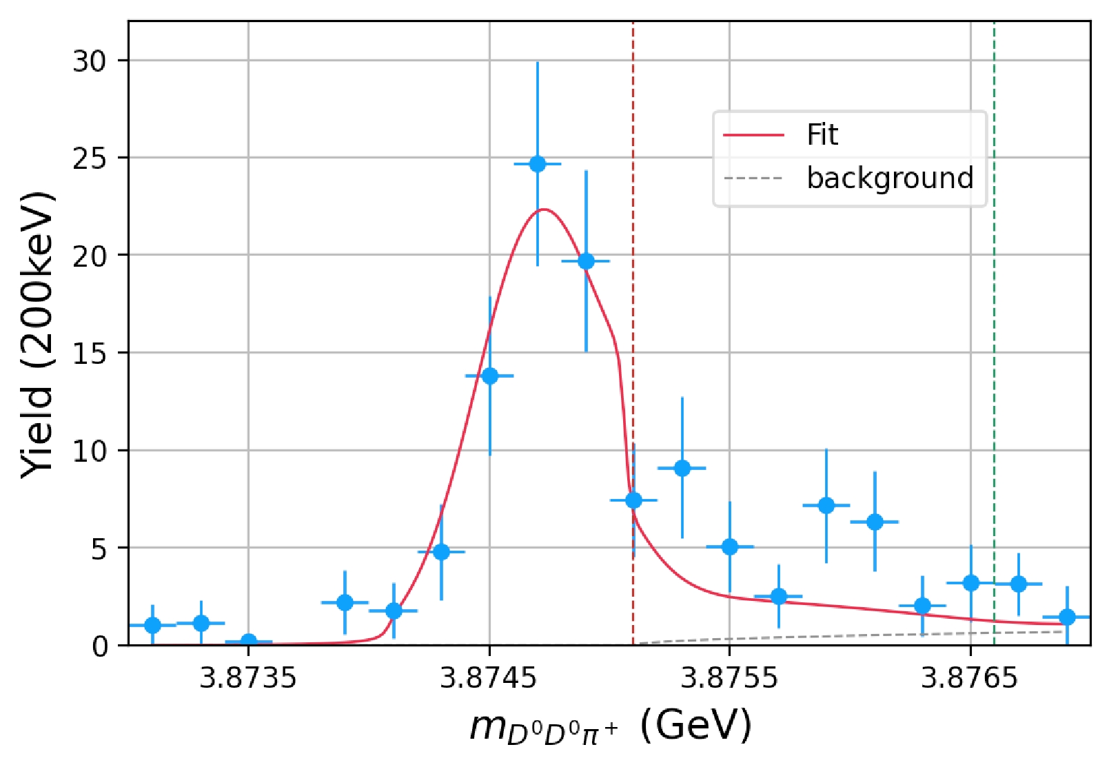
Figure 5. (color online)
$ D^0D^0\pi^+ $ final state invariant mass spectrum. The vertical purple dash line indicates the$ D^{*+}D^0 $ threshold and the green one corresponds to the$ D^{*0}D^+ $ threshold. Data obtained from Ref. [1].The pole location on the s-plane is also studied. If
$ D^{*} $ is taken as a stable particle, then$ T_{cc}^+ $ appears as a bound state pole located at$ \sqrt{s} = 3.8746 $ , that is, approximately$ 500 $ keV below the$ D^{*+}D^0 $ threshold ($ \sqrt{s} = 3.8751 $ ). As there is no accompanying virtual pole nearby, we conclude that, according to the pole counting rule,$ T^+_{cc} $ is a pure molecule composed of$ DD^* $ . However, due to the instability of$ D^* $ , the$ D^{*}D $ channel opens at the energy somewhat smaller than$ m_{D^*} + m_D $ and the decay of$ T_{cc}^+ $ takes place [14].Furthermore, invariant mass distributions for any two of three final state particles are also taken into consideration. The fit result is shown in Fig. 6. As for the
$ D^0\pi^+ $ state, which comes from$ D^{*+}D^0 $ , we take$m_{\max} = 3.8751$ GeV. As for$ D^0D^0 $ states, we take the same$m_{\max} = 3.8751$ GeV ($ \mathcal{N}' = \mathcal{N}_{DD} $ here). The$ D^+D^0 $ final state, which comes from the$ D^+D^0\pi^0 $ final state, is different. Since$ D^+D^0 $ state may come from two channels,$ D^{*+}D^0 $ and$ D^{*0}D^+ $ , they need to be considered altogether aided by isospin symmetry. Since the threshold of the second channel is higher, we take$m_{\rm max} = 3.8766\;\;\mathrm{GeV}$ , and on account of a symmetry factor${1}/{2}$ in the channel including$ D^0D^0 $ , the normalization constant here is doubled ($ \mathcal{N}' = 2\mathcal{N}_{DD} $ ). The fitting results are plotted in Fig. 7. Both invariant mass spectra ($ D^0D^0 $ and$ D^+D^0 $ ) have an incoherent background component, parametrized as a product of the two-body phase space function$ \Phi_{DD} $ and a linear function. For$ D^+D^0 $ from channel$T^+_{cc} \to D^{*0}D^+\to D^+D^0\pi^0/D^+D^0\gamma$ , because the decay channel$ D^{*0}\to D^0\gamma $ accounts for 35% of the total$ D^{*0} $ decay width, this incoherent background contribution is non-negligible and needs to be counted specially. Here, we take this estimation from Ref. [2] directly.
Figure 6. (color online)
$ D^0\pi^+ $ invariant mass spectrum from the three body final state$ D^0D^0+X $ (Data from Ref. [2]).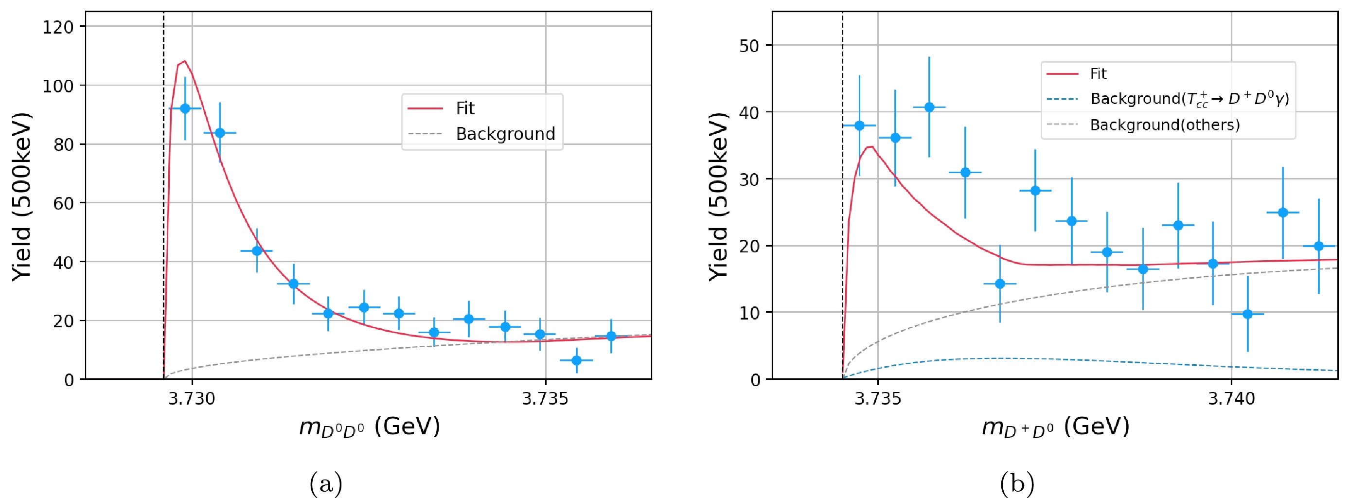
Figure 7. (color online)
$ D^0D^0 $ ($ D^+D^0 $ ) invariant mass spectrum from the three body final state$ D^0D^0+X $ ($ D^+D^0 + X $ ) [2], where the vertical dashed line indicates the$ D^{0}D^{0} $ ($ D^+D^0 $ ) threshold.Table 1. Parameters.
Finally, the fit parameters are listed in Table 1.
-
In this section, the production of
$ T^+_{cc} $ in some other methods is also analyzed to determine its compositeness. First of all, a single channel Flatté-like parametrization is used, where we do not distinguish$ D^{*+}D^0 $ and$ D^{*0}D^+ $ anymore. As in the previous calculation in Sec. II, this process is regarded as a cascade decay, as shown in Fig. 8. The propagator of$ T^+_{cc} $ is approximated by Flatté formula. The later propagator of$ D^* $ selected here is a simple Breit–Wigner amplitude form because the energy of this process is near the threshold of$ D^*D $ and its range is sufficiently small enough. Besides, the momentum dependent polynomial in the numerator is also normalized by a constant factor$ \mathcal{N} $ for convenience. Numerical calculations indicate that these approximations make little difference.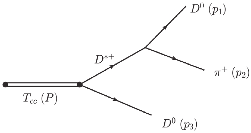
Figure 8. Cascade decay.
The total s-wave approximation amplitude about the process
$ T^+_{cc} \to D^0D^0\pi^+ $ can be written as$ \begin{aligned}[b] t= & \frac{1}{s-M^2+{\rm i} M\left(\hat g \rho(s)\right)}\\ &\times\left(\frac{1}{M_{12}^2-m_{D^{*+}}^2+{\rm i} M_{12} \Gamma_{D^{*+}}}+\frac{1}{M_{23}^2-m_{D^{*+}}^2+{\rm i} M_{23} \Gamma_{D^{*+}}}\right), \end{aligned} $

(20) where
$ \hat g $ presents the coupling strength with$ D^*D $ . The doubling of the kinetic variables of the$ D^* $ propagator is due to the indistinguishability of$ D\pi $ in the three-body final state, and the symmetry factor$ \dfrac{1}{2} $ is absorbed by the total normalization$ \mathcal{N} $ . By this parametrization, we make the energy resolution convolution as that before and fit the three-body decay width and two-body invariant mass spectra at the same time using the previous Eqs. (17) and (19). It is worth pointing out that under normal conditions, it will form a divergent peak because of the zero partial decay width. However, if we regard$ D^* $ as an unstable particle, in other words, if the amplitude can develop an imaginary part when the energy has not yet reached the$ D^*D $ threshold, the peak is not divergent anymore. We can use the same stratagem as Eq. (13) to treat ρ in Eq. (20), or more simply take the value$ m_{D^*} $ in ρ with an imaginary part$ \Gamma_{D^*} $ . This selection does not affect the result except for the goodness of fit. Here, we take the latter scenario. The results of the combined fit are shown in Fig. 9.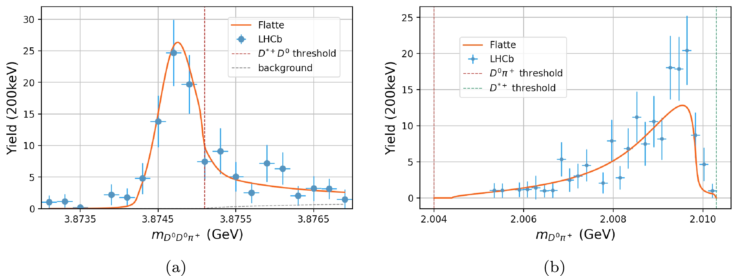
Figure 9. Three-body and two-body invariant mass spectrum.
We list the corresponding parameters in Table 2, and the pole structure of the Flatté amplitude is displayed in Fig. 10.
$ \chi^2/d.o.f $ 

$ \hat g $ 

M $ 0.81 $ keV

$ 0.075\pm 0.015 $ 

$ 3874.1\pm 0.2 $ MeV

Table 2. Fit parameter.
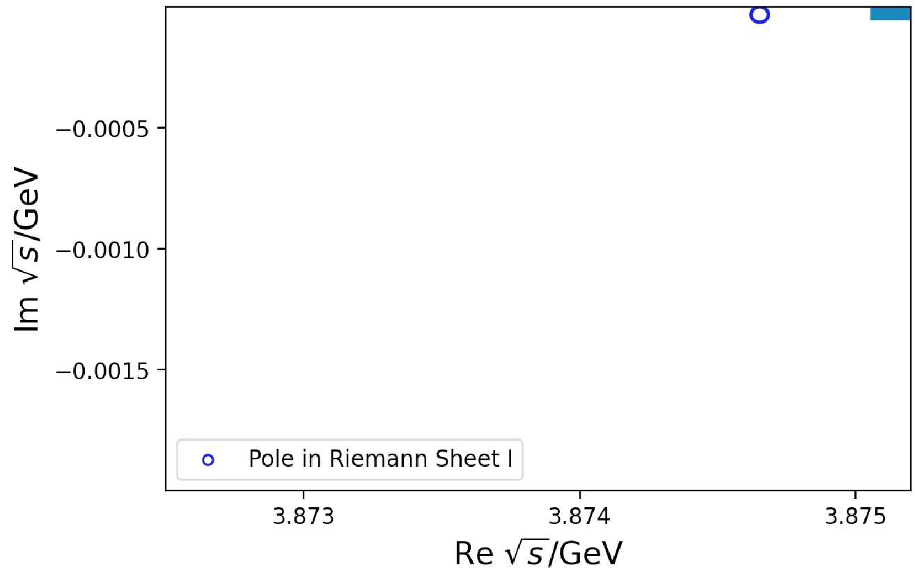
Figure 10. Pole structure of flatté amplitude.
Furthermore, according to the Flatté-like parametrization, it is natural to calculate the probability of finding an 'elementary' state in the continuous spectrum by the spectral density function [26]
$ \omega(E)=\frac{1}{2 \pi} \frac{\tilde{g} \sqrt{2 \tilde{M} E} \theta(E)+\tilde{\Gamma}_0}{\left|E-E_f+\dfrac{\mathrm{i}}{2} \tilde{g} \sqrt{2 \tilde{M} E} +\dfrac{\mathrm{i}}{2} \tilde{\Gamma}_0\right|^2}, $

(21) where
$ E = \sqrt{s} - m_{D^*D} $ ,$ E_f = M - m_{D^*D} $ ,$ \tilde{M} $ is the reduced mass of$ D^*D $ , θ is the step function at threshold,$ \tilde{g} = 2 \hat{g} / m_{D^*D} $ is the dimensionless coupling constant of the concerned coupling mode, and$ \tilde{\Gamma}_0 $ is the constant partial width for the remaining couplings. By integrating it with a cut off (usually comparable to the total decay width$ \sim \Gamma $ ), the possibility of finding an 'elementary' state in the final state is$ \mathcal{Z}=\int_{E_{\min }}^{E_{\max }} \omega(E) \mathrm{d} E. $

(22) Considering that no other channels are coupling with
$ T^+_{cc} $ under the$ D^*D $ threshold, the$ \tilde{\Gamma}_0 $ here should be set to zero. In this case, the integrated results in different sections are as follows.The result suggests that in a simple single channel Flatté-like parametrization framework,
$ T^+_{cc} $ is a pure molecular state. This is in agreement with the result of Ref. [27], obtained using an effective range expansion approximation. Our result is much more definite than that obtained in Ref. [2].Furthermore, the compositeness may also be discussed from the production rate of a particle. The cross section relation between the confined states
$ \Xi_{cc} $ ($ ccu/ccd $ ) [28] and$ T^+_{cc} $ can be obtained from the experiment. Since 2016, these two sets of experimental data are both collected under the same experimental conditions, such as transverse momentum truncation$ p_T $ and luminance$9~\rm fb^{-1}$ . After taking account of the detection efficiency and branching fraction differences [29], there is an approximate relation$ \frac{\sigma(pp\to T^+_{cc})}{\sigma(pp\to \Xi_{cc})} \sim \frac{1}{3} \times \frac{1}{10}. $

(23) If we agree that there exists a universal ratio between the
$ (Q/QQ)q $ and$ (Q/QQ)qq $ productivities in high energy collision [30], where Q represents a heavy quark and q is a light quark, we can obtain a factor$ 1/3 $ , which means that catching two light quarks is always more difficult, that is,$ \sigma(pp\to \Xi_{cc}) \simeq 3 \sigma(pp\to (cc\bar{u}\bar{d})) $ . Thus, the ratio between the cross sections of the observed$ T^+_{cc} $ and the hypothetical tetraquark can be obtained as$ \frac{\sigma(pp\to T^+_{cc})}{\sigma(pp\to (cc\bar{u}\bar{d}))} \sim \frac{1}{10}. $

(24) It is also possible to estimate the different orders of magnitude of the theoretical cross sections between the `elementary' and `molecular' pictures of
$ T^+_{cc} $ . Because the$ X(3872) $ resonance has analogous characteristics [31, 32] (e.g., binding energy and quark composition), some comparisons have been made about these orders of magnitude for$ X(3872) $ [33, 34]. If one can borrow the discussions here, it can be estimated that approximately for$ T^+_{cc} $ $ \frac{\sigma(pp\to (c\bar{u})(c\bar{d}))}{\sigma(pp\to (cc\bar{u}\bar{d}))} \sim \mathcal{O}(10^{-2})-\mathcal{O}(10^{-3}). $

(25) A similar result was also obtained in [35]. By comparing Eq. (24) and Eq. (25), one can find that the production of
$ T^+_{cc} $ just falls in between two different cases. However, this analysis depends on some uncertain assumptions and is not quite reliable. In Ref. [36], the production cross section for$ T_{cc} $ as a molecule was estimated to be approximately an order of magnitude higher than that as a tetraquack, which creates more confusion. Thus, using the production argument cannot provide a clear conclusion on the nature of$ T^+_{cc} $ . On the contrary, the analysis provided in this paper, for example in Table 3, clearly indicates the molecular nature of$ T^+_{cc} $ .$ [M-\Gamma, M+\Gamma] $ 

$ [M-2\Gamma, M+2\Gamma] $ 

$ [M-3\Gamma, M+3\Gamma] $ 

$ \sim $ 0

$ \sim $ 0

0.01 Table 3. Spectral density function integrating
$ \mathcal{Z} $ . -
In this work, we study the nature of
$ T^+_{cc} $ using different methods. First, an effective field theory Lagrangian with two channels ($ D^{*+}D^0 $ and$ D^{*0}D^+ $ ) combined with a K-matrix approach is used to describe the$ T^+_{cc}\to D^0D^0\pi^+ $ process. The three-body and two-body invariant mass spectrum can be fitted well at the same time. The numerical fit results reveal that vector meson exchanges are more important than π exchanges and contact interactions. Second, the Flattè formula is used to study the same problem. Both approaches suggest that$ T^+_{cc} $ is definitely a pure molecular state composed of$ D^*D $ , in agreement with many of the results found in the literature, but on a much more confident level. -
We are grateful to E. Oset for the helpful comments and proofreading, and would also like to thank Hao Chen for the careful reading of the manuscript and helpful discussions.
Some remarks on compositeness of ${{\boldsymbol T}^{\bf +}_{\boldsymbol{cc}}} $
- Received Date: 2023-10-26
- Available Online: 2024-04-15
Abstract: Recently, the LHCb experimental group found an exotic state


 DownLoad: