


 Abstract
 HTML
HTML Reference
 Related
 PDF
PDF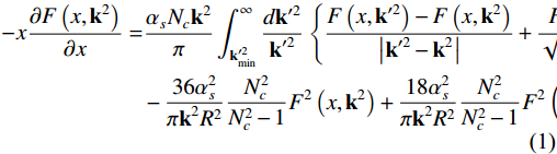


 DownLoad:


-
In the framework of perturbative quantum chromodynamics (pQCD), the understanding and prediction of parton distribution functions (PDFs) in protons can be achieved through the utilization of QCD evolution equations. The well-established Dokshitzer-Gribov-Lipatov-Altarelli-Parisi (DGLAP) evolution equation [1−3] is applied to describe the growth of partons at high
Q2 , whereas the Balitsky-Fadin-Kuraev-Lipatov (BFKL) equation [4−9] provides insights into gluon splitting in the small-x region [10].Nonetheless, both DGLAP and BFKL equations exhibit unbounded growth of the gluon density, which violates either the unitary or the Froissart bound [11]. To address this issue, higher-order corrections must be taken into consideration to regulate this uncontrolled growth. Specifically, in regions of high density, gluons recombine, and such recombination effects become particularly significant in the near-unitarity limit, eventually leading to saturation. The Color Glass Condensate (CGC) effective theory serves as a potent and valuable tool for describing the saturation phenomenon [12−15]. Within the framework of CGC, the Jalilian-Marian-Iancu-McLerran-Weigert-Leonidov-Kovner (JIMWLK) renormalization group equation [12, 16−18] was introduced to account for small-x QCD evolution incorporating nonlinear corrections. The mean-field approximation of the JIMWLK equation, known as the Balitsky-Kovchegov (BK) equation [19−21], serves as a nonlinear extension of the BFKL equation. By considering the dipole scattering amplitude, the BK equation bridges the gap between the unsaturated and saturated regions.
Furthermore, an alternative approach for modifying the gluon DGLAP evolution equation has been proposed by the Gribov-Levin-Ryskin and Mueller-Qiu (GLR-MQ) equation [22−26]. However, it is worth noting that the derivation of the GLR-MQ equation relies on the application of AGK-cutting rules [27]. As highlighted in Ref. [28], the employment of AGK-cutting rules in the GLR-MQ equation presents certain limitations and drawbacks. Notably, the GLR-MQ equation overlooks the antishadowing corrections associated with gluon recombination. To address these limitations, Zhu, Ruan, and Shen revisited parton recombination within the framework of the QCD evolution equation using time-ordered perturbation theory (TOPT). This led to the derivation of the modified BFKL equation (MD-BFKL) and the modified DGLAP equation (MD-DGLAP) [29, 30]. Importantly, both antishadowing and shadowing effects are considered within these modified equations, ensuring the preservation of momentum conservation throughout the QCD recombination processes [31−34].
In Ref. [30], the numerical solution of the MD-BFKL equation demonstrated that the anti-shadowing effect has a sizable impact on the gluon distribution. Therefore, it is meaningful to obtain an analytic unintegrated gluon distribution from the MD-BFKL equation. In recent years, a solution of the kinematic-constraint improved MD-BFKL equation (KC-MD-BFKL) was obtained [35] in the near saturation region. In fact, based on variable transformation, the MD-BFKL equation can be transformed into a BK-like equation [30]. The BFKL kernel in the BK-like equation can be expanded to a differential kernel as performed for the BK equation [36−38], which is connected to the Fisher-Kolmogorov-Petrovsky-Piscounov (FKPP) equation [39−41]. Therefore, the MD-BFKL equation can be rewritten as an analytically solvable nonlinear partial differential equation under the diffusive approximation. In this work, we solved this nonlinear partial differential equation analytically with and without the inclusion of the anti-shadowing effect. In our following calculations, it is shown that the anti-shadowing correction plays an important role for unintegrated gluon distribution.
The arrangement of this article is as follows. In Sec. II, we briefly introduce the MD-BFKL equation and its transformation form, the BK-like equation. In Sec. III, the analytic solutions of the BK-like equation with and without the anti-shadowing effect are obtained. Sec. IV presents the results of fitting to the gluon distribution function using our solutions. Sec. V includes the discussion and summary.
-
In Ref. [30], a unitarized MD-BFKL equation incorporating both shadowing and anti-shadowing corrections of the gluon recombination is shown as
−x∂F(x,k2)∂x=αsNck2π∫∞k′2mindk′2k′2{F(x,k′2)−F(x,k2)|k′2−k2|+F(x,k2)√k4+4k′4}−36α2sπk2R2N2cN2c−1F2(x,k2)+18α2sπk2R2N2cN2c−1F2(x2,k2), (1) where
F(x,k2) is the unintegrated gluon distribution [42−45],αs is the coupling constant,Nc is the color number, and R is the effective correlation length of two recombination gluons.R≈5GeV−1 stands for the hadronic characteristic radius, whereasR≈2GeV−1 stands for the hot spot radius [46]. In this work, R is determined by fitting the gluon distribution function. The linear part in Eq.N(x,k2)≡27αs4k2R2F(x,k2).
(2) With this definition, Eq.
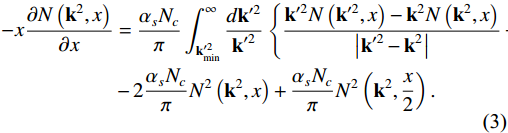
−x∂N(k2,x)∂x=αsNcπ∫∞k′2mindk′2k′2×{k′2N(k′2,x)−k2N(k2,x)|k′2−k2|+k2N(k2,x)√k4+4k′4}−2αsNcπN2(k2,x)+αsNcπN2(k2,x2).
(3) Here we refer to Eq. (3) as the BK-like equation, which exhibits a comparable structure to the conventional BK equation in momentum space. Therefore, N can be called "dipole scattering amplitude".
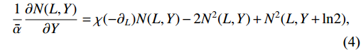
Equation (3) can now be simplified into an analytically solvable form. It is well-known that the BFKL kernel in Eq. (3) can be transformed into a differential kernel [20]. Therefore, Eq. (3) can be written as
1ˉα∂N(L,Y)∂Y=χ(−∂L)N(L,Y)−2N2(L,Y)+N2(L,Y+ln2),
(4) where
ˉα=αsNcπ ,Y=ln1x ,L=ln(k2k20) ,k20 is an arbitrary scale, andχ(−∂L) is the BFKL kernel [4, 7, 8],χ(−∂L)=2ψ(1)−ψ(−∂L)−ψ(1+∂L).
(5) χ(−∂L) can be expanded around the critical pointγc [38],χ(−∂L)=P∑p=0χ(p)(γc)p!(−∂L−γc)p=P∑p=0(−1)pAp∂pL.
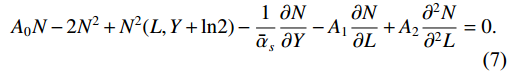
(6) Expanding
χ(−∂L) to the second order (the diffusive approximation), Eq. (4) is rewritten as [36−38]A0N−2N2+N2(L,Y+ln2)−1ˉαs∂N∂Y−A1∂N∂L+A2∂2N∂2L=0.
(7) Here,
A0 ,A1 , andA2 are the expansion coefficients. For the sake of simplicity, we do not write the default variables L and Y for N. In the next section, we simplifyN2(L,Y+ln2) in Eq. (7) to obtain the analytical solution. -
In this section, the detailed description of solving Eq. (7) with fixed coupling is provided. To consider the impact of anti-shadowing correction, we take into account two strategies for the nonlinear parts:
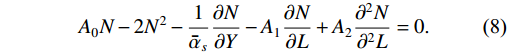
(I) The anti-shadowing term is canceled directly. Only the shadowing effect is considered. Therefore, Eq. (7) is rewritten as
A0N−2N2−1ˉαs∂N∂Y−A1∂N∂L+A2∂2N∂2L=0.
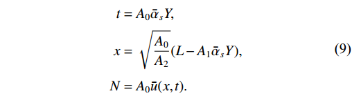
(8) By the variable substitution,
t=A0ˉαsY,x=√A0A2(L−A1ˉαsY),N=A0ˉu(x,t).
(9) Equation (8) is transformed into the FKPP equation,
ˉuxx−ˉut+ˉu−2ˉu2=0.
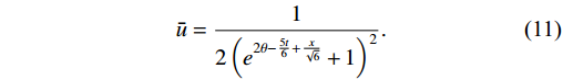
(10) Equation (10) means that
F(x.k2)k2 satisfies the reaction-diffusion FKPP equation when only the shadowing term is retained. It is straightforward to obtain its solution with the homogeneous balance method [47],ˉu=12(e2θ−5t6+x√6+1)2.
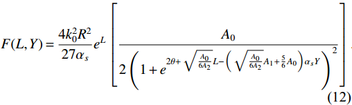
(11) Here, θ is an arbitrary constant. Naturally, the unintegrated gluon is obtained:
F(L,Y)=4k20R227αseL[A02(1+e2θ+√A06A2L−(√A06A2A1+56A0)αsY)2].
(12) (II) Both shadowing and anti-shadowing effects are retained. In this situation, the only difficulty in obtaining analytic solutions is how to deal with
N2(L,Y+ln2) . When we consider that Eq. (7) has a traveling wave solution, the equation only depends on a single variableτ=L+bY , where b is an arbitrary constant. Therefore,N2(L,Y+ln2) is written asN2(τ+b⋅ln2) . Then,N2(τ+b⋅ln2) is expanded in a Taylor series around τ and retained up to the first order,N2(τ+b⋅ln2)≈N2(τ)+b⋅ln2∂N2(τ)∂τ.
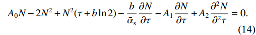
(13) Using variable τ, Eq. (7) is rewritten as
A0N−2N2+N2(τ+bln2)−bˉαs∂N∂τ−A1∂N∂τ+A2∂2N∂2τ=0.
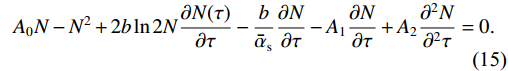
(14) Then, when
N2(τ+bln2) is replaced by Eq. (13), Eq. (14) is approximated asA0N−N2+2bln2N∂N(τ)∂τ−bˉαs∂N∂τ−A1∂N∂τ+A2∂2N∂2τ=0.
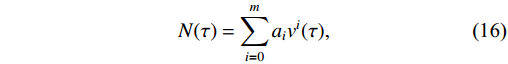
(15) Equation (15) can be solved by using the homogeneous balance method [48]. One can suppose that
N(τ) can be expanded toN(τ)=m∑i=0aivi(τ),
(16) where
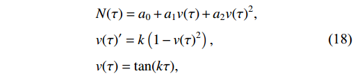
ai is the expansion coefficient andv(τ) is the expansion function. The condition forv(τ) isdvdτ=k(1−v2) . Using the homogeneous balance method to balance the highest power of v from∂2N/∂2τ with the highest power of v from the nonlinear termsN2 , we can obtainm+2=2m.
(17) It is obvious that
m=2 . Therefore, the form of the solution of Eq. (15) isN(τ)=a0+a1v(τ)+a2v(τ)2,v(τ)′=k(1−v(τ)2),v(τ)=tan(kτ),
(18) where
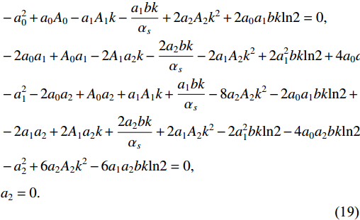
a0 ,a1 ,a2 , and k are parameters to be determined. Then, Eq. (18) is substituted into Eq. (15) and the coefficients ofvi are set to zero,−a20+a0A0−a1A1k−a1bkαs+2a2A2k2+2a0a1bkln2=0,−2a0a1+A0a1−2A1a2k−2a2bkαs−2a1A2k2+2a21bkln2+4a0a2bkln2=0,−a21−2a0a2+A0a2+a1A1k+a1bkαs−8a2A2k2−2a0a1bkln2+6a1a2bkln2=0,−2a1a2+2A1a2k+2a2bkαs+2a1A2k2−2a21bkln2−4a0a2bkln2+4a22bkln2=0,−a22+6a2A2k2−6a1a2bkln2=0,a2=0.
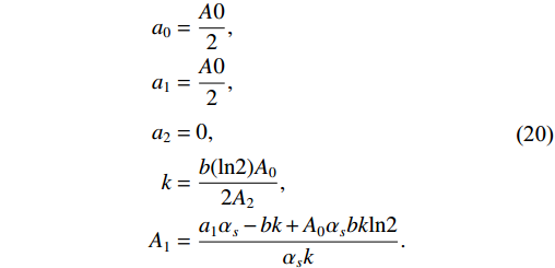
(19) By solving Eq. (19), we obtain a suitable set of parameter values:
\begin{aligned} a_0&=\frac{A0}{2},\\ a_1&=\frac{A0}{2},\\ a_2&= 0,\\ k&=\frac{b(\mathrm{ln}2)A_0}{2A_2},\\ A_1&=\frac{a_1\alpha_s-bk+A_0\alpha_sbk\mathrm{ln}2}{\alpha_s k}. \end{aligned}
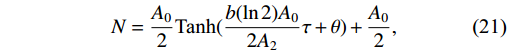
(20) Therefore, the solution of Eq. (15) is obtained as follows:
{N}=\frac{A_0}2\text{Tanh}(\frac{{b}(\ln2){A}_0}{2{A}_2}\tau+\theta)+\frac{{A}_0}2,
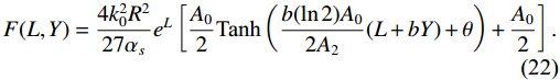
(21) where θ is a free parameter. Using the definition in Eq. (2), the unintegrated gluon distribution is written as
F({L},{Y})=\frac{4k_0^2 R^2}{27\alpha_s}{\rm e}^{L}\left[\frac{A_0}2\text{Tanh} \left(\frac{{b}(\ln2){A}_0}{2{A}_2}(L+bY)+\theta \right)+\frac{{A}_0}2\right].
(22) Generally, the values of
A_0 ,A_1 , andA_2 are determined by the saddle point in the diffusive approximation. However, to enhance the description of the gluon distribution, we relaxed this constraint. Therefore, in the next section, the parameters in Eq. (12) and Eq. (22) are determined by fitting to the gluon distribution from the database. The gluon distribution exhibits variability across different databases. For this study, CT18NLO was selected because it considers the saturation effect in small-x by introducing the x dependent scale. -
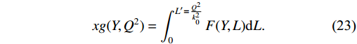
The relation of the unintegrated gluon distribution
F({Y},{L}) with the integrated gluon distribution{xg}({Y},{Q^2}) is{xg}({Y},{Q^2})=\int_{0}^{{L'}=\frac{{Q^2}}{k^2_0}}F({Y},{L}){\mathrm{d}L}.
(23) To obtain a definite solution that can match the gluon distribution function, the free parameters in Eq. (12) and Eq. (22) are acquired by fitting to CT18NLO [49, 50]. As we are focused on the properties of gluon distribution in the small-x region, the fitting range of Y is set from 6 to 12. The fitting range of
Q^2 is from 4\mathrm{GeV^2} to 100\mathrm{GeV^2} . We set\alpha_s=0.2 andk_0^2=0.04~\, \mathrm{GeV^2} . The coefficients from fitting to CT18NLO are listed in Table 1. The parameter values that are not presented in Table 1 can be obtained through the relationship in Eq. (20).Shadowing and anti-shadowing Shadowing A_0 
0.517 \pm \,0.010 
1.507 \pm\,0.020 
A_1 
− 0.308 \pm\,0.023 
A_2 
0.137 \pm \,0.002 
0.541 \pm\,0.007 
b −0.431 \pm \,0.003 
− R 2.432 \pm \,0.030 
2.367 \pm\,0.029 
\chi^2/dof 
37.660/(1260-5) 
36.420/(1260-5) 
As shown in Fig. 1, the fitting results of the two situations for integrated gluon distribution
xg(Y,Q^2) are presented atY=6 ,Y=8 ,Y=10 , andY=12 , respectively. Further, Fig. 2 demonstratesxg(Y,Q^2) as a function of Y atQ^2=10~\,\mathrm{GeV^2} ,Q^2=20~\,\mathrm{GeV^2} ,Q^2=40~\,\mathrm{GeV^2} , andQ^2=80~\,\mathrm{GeV^2} , respectively. Our solutions can be related to the gluon distribution by using Eq. (23). The solid lines denote that both shadowing and anti-shadowing effects are considered. The dashed lines indicate that only the shadowing effect is included. Despite fitting the same gluon data, we can still find differences between the gluon distribution functions with and without the anti-shadowing effect asQ^2 increases, especially in the higher Y region. When Y is larger, the total effect from the shadowing and anti-shadowing terms is more obvious, which means that the recombination effect becomes increasingly important when gluons approach or enter the saturation region. As gluons approach or enter the deep saturation region, the dominant effect is the shadowing resulting from the recombination process, which suppresses the growth of gluons to maintain unitarity. When gluons move away from the deep saturation region, the contribution of the anti-shadowing effect from the recombination process is visible. The shadowing effect is weakened by the anti-shadowing effect. Therefore, the value of gluon distribution with the anti-shadowing effect is higher than that without the anti-shadowing effect asQ^2 increases.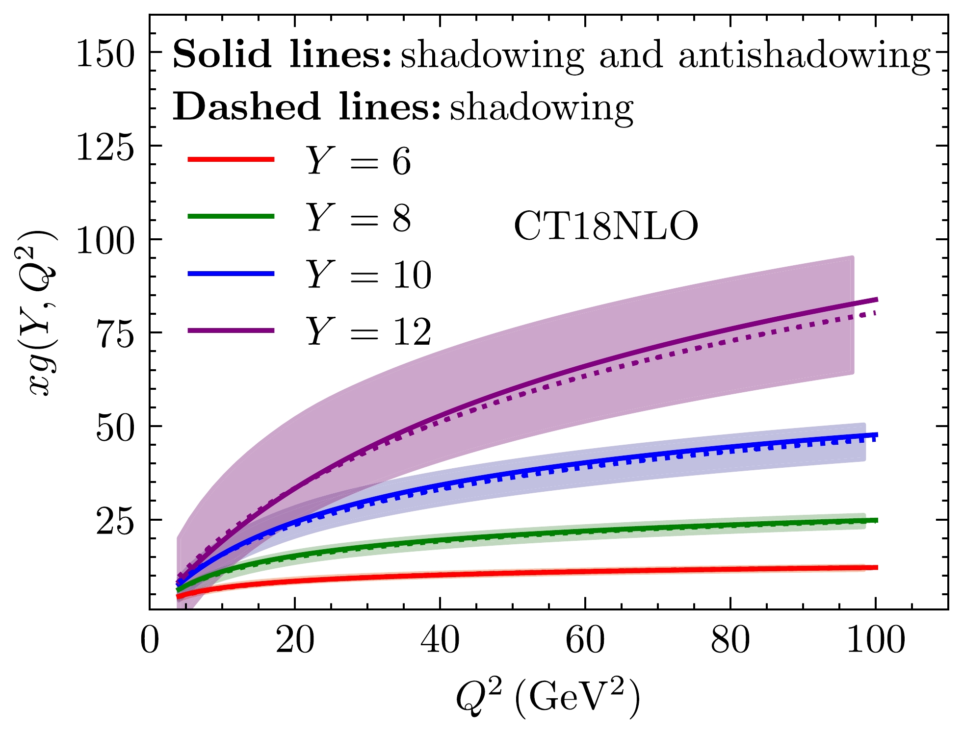
Figure 1. (color online) Gluon distribution function fitted to CT18NLO [49, 50] using Eq. (23) at
Y=6 ,Y=8 ,Y=10 , andY=12 (from bottom to top). The color bands stand for the CT18NLO gluon data with uncertanties. The solid lines denote that both shadowing and anti-shadowing effects are considered. The dashed lines indicate that only the shadowing effect is included.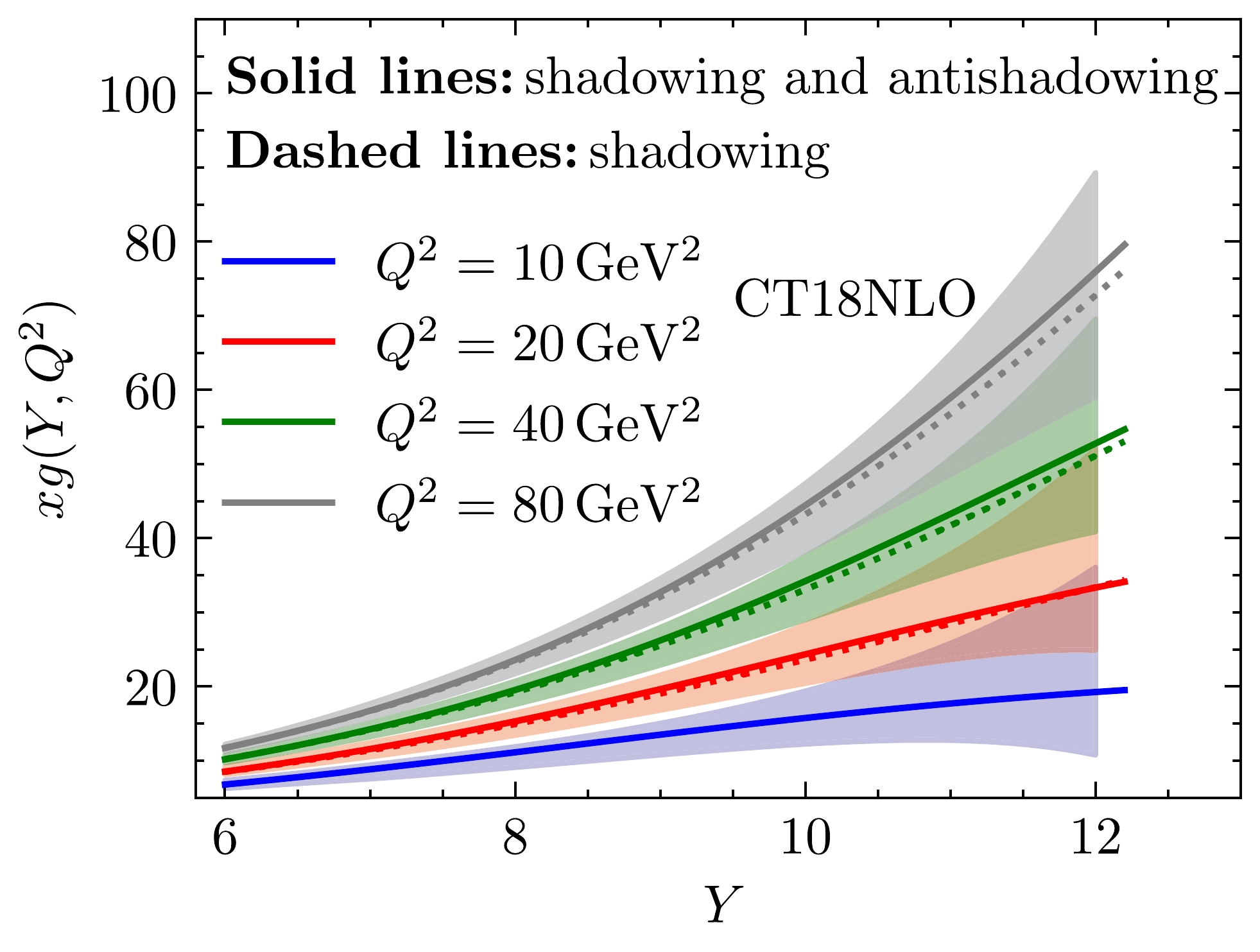
Figure 2. (color online) Gluon distribution function fitted to CT18NLO [49, 50] using Eq. (23) at
Q^2=10~\,\mathrm{GeV^2} ,Q^2=20~\,\mathrm{GeV^2} ,Q^2=40~\,\mathrm{GeV^2} , andQ^2=80~\,\mathrm{GeV^2} (from bottom to top). The color bands stand for the CT18NLO gluon data with uncertanties. The solid lines denote that both shadowing and anti-shadowing effects are considered. The dashed lines indicate that only the shadowing effect is included.The unintegrated gluon distributions
F({Y,L}) with and without the anti-shadowing effect are shown in Fig. 3 and Fig. 4. Figure 3 illustratesF({Y,L}) as a function of L atY=6 ,Y=8 ,Y=10 , andY=12 , respectively. Figure 4 demonstrates the behavior ofF({Y,L}) with Y atL=8 ,L=12 ,L=16 , andL=20 , respectively. For the evolution of unintegrated gluon distributions, the impact of the anti-shadowing effect is significant. In a large L, the unintegrated gluon distribution with the anti-shadowing effect decreases more slowly. When the gluon moves away from the saturation, the anti-shadowing effect gradually increases its effect as L becomes larger. Therefore, the anti-shadowing correction is important for the gluon distribution.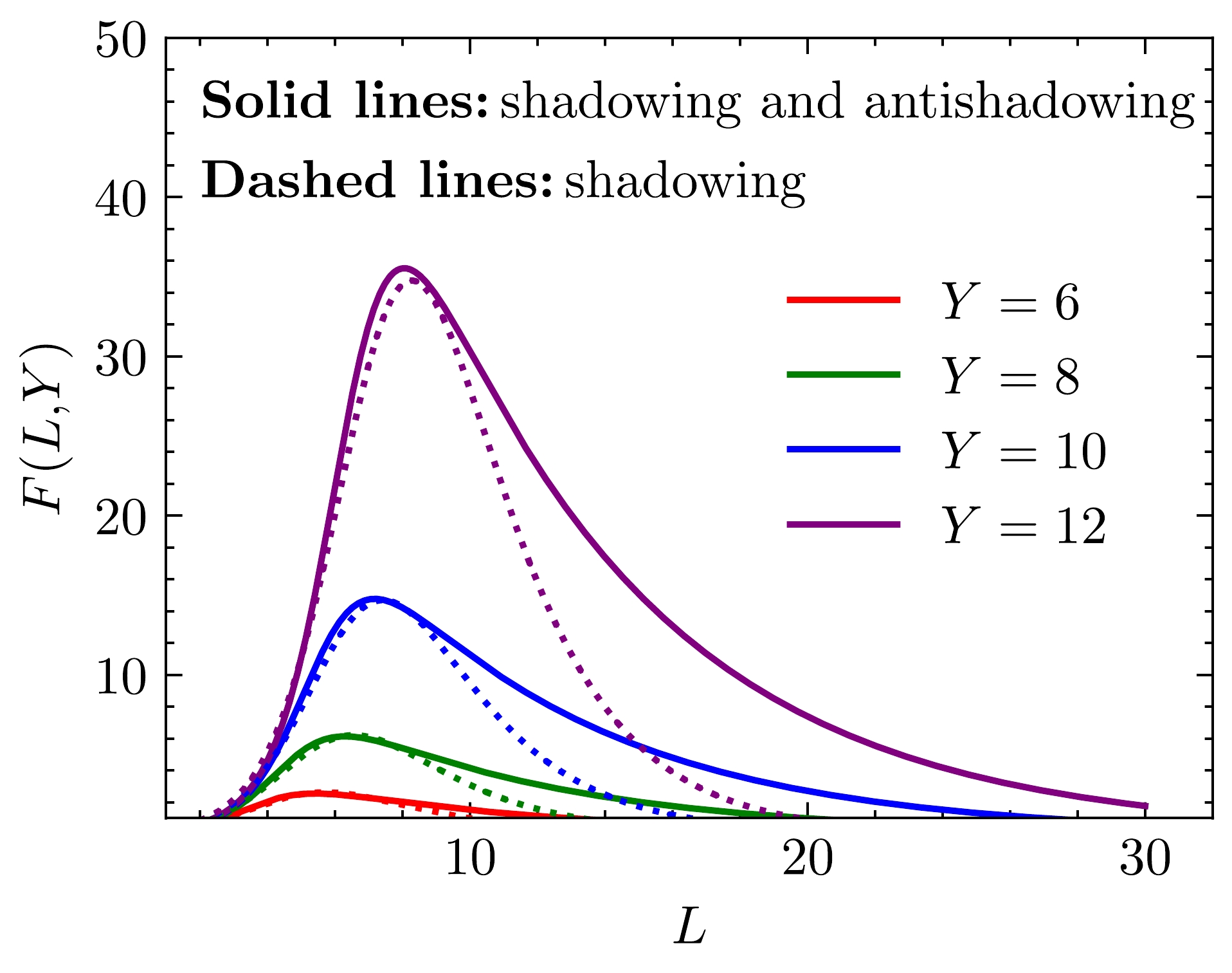
Figure 3. (color online) Comparison of the unintegrated gluon distribution function including shadowing and anti-shadowing effects with the unintegrated gluon distribution function only including the shadowing effect as a function of Y at
Y=6 ,Y=8 ,Y=10 , andY=12 (from bottom to top). The solid lines denote that both shadowing and anti-shadowing effects are considered. The dashed lines indicate that only the shadowing effect is included.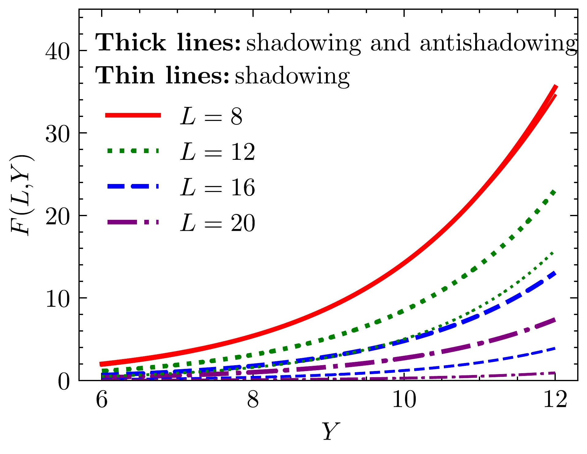
Figure 4. (color online) Comparison of the unintegrated gluon distribution function including shadowing and anti-shadowing effects with the unintegrated gluon distribution function only including the shadowing effect as a function of Y at
L=8 ,L=12 ,L=16 , andL=20 , respectively. The thick lines represents the situation where both shadowing and anti-shadowing effects are considered. The thin lines stand for the situation where only the shadowing effect is included.It should be noted that,
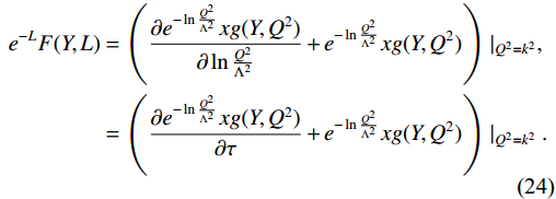
{{\rm e}^{-L}}F({L},{Y})\propto N({L},{Y}) from Eq. (2) has scaling characteristic when the running coupling constant is fixed. In other words,{{\rm e}^{-L}}F({L},{Y}) is a function of only one dimensionless variable\tau={L}+b{Y} . For the situation where only the shadowing effect is considered,\tau={L}+b_{sh}{Y} , whereb_{sh}=-(A_1+5\sqrt{\frac{A_0A_2}{6}})\alpha_s=- 0.4302 , which is close to the value in the case with anti-shadowing (see Table 1). In general, as shown in Fig. 5, the difference in scaling behavior of the two solutions is not obvious. Actually, the scaling property of{{\rm e}^{-L}}F({L},{Y}) implies that{{\rm e}^{-\ln {Q^2}/{\Lambda^2}}}xg(x,Q^2) has geometric scaling characteristic when\alpha_s is fixed [25, 51]. However,\alpha_s can only be considered a constant whenQ^2 is large. The correlation of geometric scaling properties between the unintegrated and integrated gluon distributions is obvious in the differential relationship.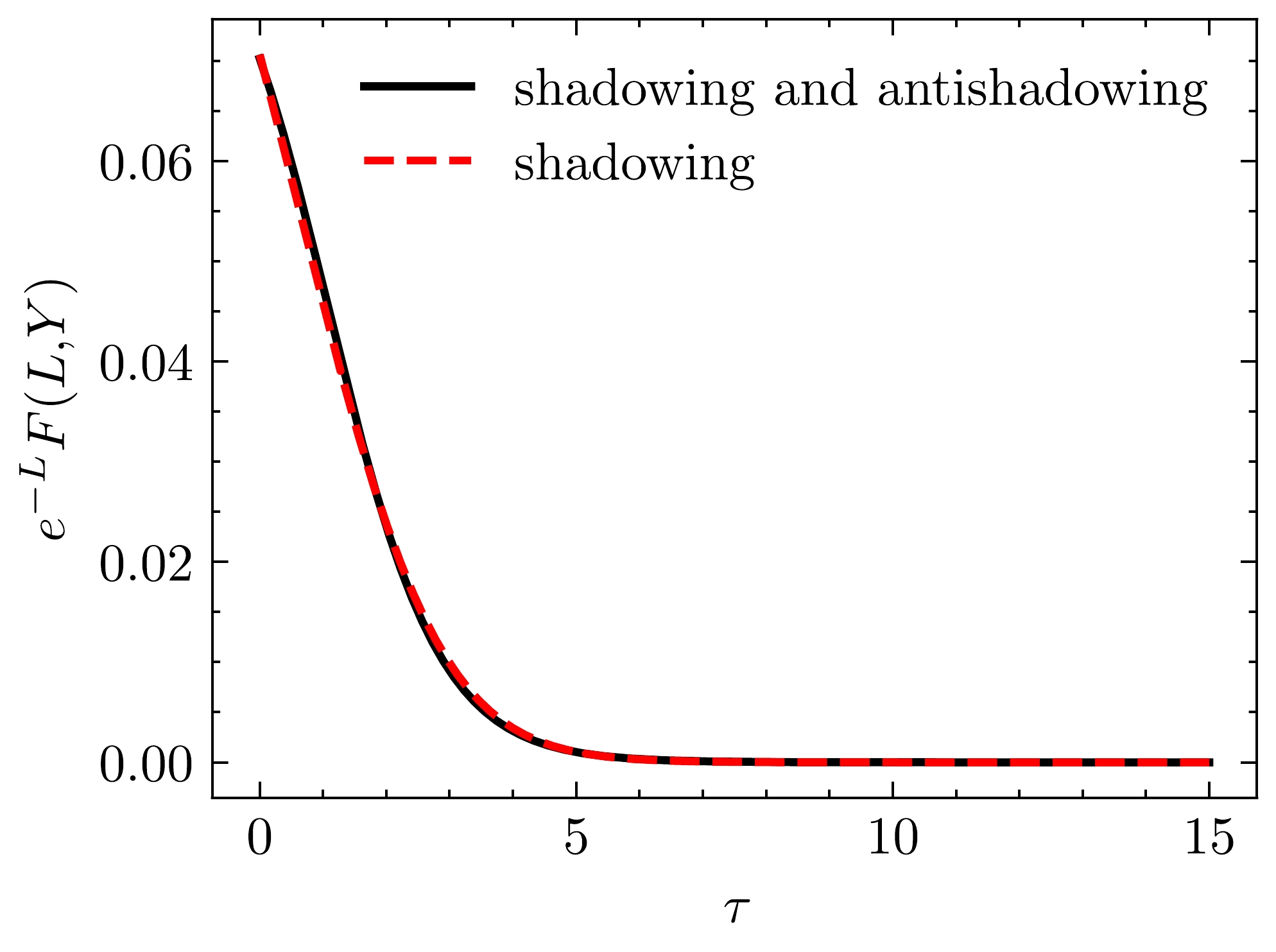
Figure 5. (color online)
{\rm e}^{-{L}}F({L},{Y}) as a function of only one dimensionless variable τ. The solid line denotes that both shadowing and anti-shadowing effects are considered. The dashed line indicates that only the shadowing effect is included\begin{aligned} {\rm e}^{-L}F(Y,L)&=\left( \frac{\partial {\rm e}^{-\ln\frac{Q^2}{\Lambda^2}}xg(Y,Q^2)}{\partial \ln\frac{Q^2}{\Lambda^2}}+{\rm e}^{-\ln\frac{Q^2}{\Lambda^2}}xg(Y,Q^2)\right)\bigg|_{Q^2=k^2},\\ &=\left( \frac{\partial {\rm e}^{-\ln\frac{Q^2}{\Lambda^2}}xg(Y,Q^2)}{\partial \tau}+{\rm e}^{-\ln\frac{Q^2}{\Lambda^2}}xg(Y,Q^2)\right)\bigg|_{Q^2=k^2}. \end{aligned}
(24) The scaling behavior of
{\rm e}^{-L}F(Y,L) , comes from the geometric scaling of gluon distribution from CT18NLO. As shown in Fig. 1 and Fig. 2, the difference between two situations for{\rm e}^{-\ln{Q^2}/{\Lambda^2}}xg(Y,Q^2) is small. The values of parameter b in these two situations are nearly identical, indicating that the discrepancy in scaling behavior between the two solutions is not significant. -
In this study, the MD-BFKL equation is transformed to the BK-like equation by using the relationship between "dipole scattering amplitude" and unintegrated gluon distribution. The BK-like equation arises from the expansion of the BFKL kernel to second order using the diffusive approximation, resulting in a nonlinear partial differential equation. By considering the nonlinear term,
N(\frac{x}{2},k^2) , in two strategies (with and without anti-shadowing), we derive solutions for the MD-BFKL equation using the homogeneous balance method.To investigate the impact of the anti-shadowing effect, we compare and contrast the obtained solutions, successfully determining their parameters by fitting them to the CT18NLO gluon distribution function in the small-x region. Our findings, illustrated in Fig. 1 and Fig. 2, reveal that the gluon distribution without the anti-shadowing effect exhibits a gentler growth as
Q^2 and Y increase. Fig. 3 and Fig. 4 further demonstrate a significant disparity between the unintegrated gluon distributions with and without the anti-shadowing effect, with the latter showing a slower decrease in large L values. This disparity becomes more pronounced with an increase in Y.In addition, the scaling behavior of
{{\rm e}^{-L}}F({L},{Y}) is presented. In fact, the scaling properties of{{\rm e}^{-L}}F({L},{Y}) reflect the geometric scaling property of{\rm e}^{-\ln{Q^2}/{\Lambda^2}}xg(Y,Q^2) when\alpha_s is fixed. In conclusion, our obtained solutions provide valuable insights into the nature of gluon distributions and pave the way for future phenomenological studies.
| Shadowing and anti-shadowing | Shadowing | |
| 0.517 | 1.507 |
| − | 0.308 |
| 0.137 | 0.541 |
| b | −0.431 | − |
| R | 2.432 | 2.367 |
| | |


