-
In the past several decades, observational and theoretical research has been widely conducted to explain the dynamics of the universe, and the outcome has been precisely consistent with the standard cosmological model, called the ΛCDM model, which is based on the theory of General Relativity (GR) [1]. On the contrary, observations of the cosmic microwave background radiation (CMBR) from different studies have provided significant facts on the evolution and development of the universe [2−7]. However, many challenging issues, such as the flatness and horizon problems, remain unsolved within the parameters of standard cosmological data [8]. To address these issues, it has been suggested to consider an era of accelerated expansion in the initial stage of the universe's evolution, called "cosmic inflation" [9−12]. In
1981 , the first model of inflation was proposed by Guth [10] and Sato [13], but their model (old inflation) did not adequately explain the universe's inhomogeneity due to bubble collision at the end of inflation. Linde [11] and Albrecht and Steinhardt [12] proposed an updated version (so-called new inflation) in1982 , but it did not address the problem of taking enough time in a false vacuum. Linde later proposed chaotic inflation [14], which suggests that the universe is produced in regions with sufficient inflation. These models have different implications regarding the thermal equilibrium of the early universe.Cosmic inflation can be effectively described by considering a scalar field
(\varphi) , dubbed as an "inflaton" that is determined by a particular effective potential. The quantum fluctuations generated due to inflaton field can pave the way towards exponential growth, explaining how large-scale structures form. The inflationary mechanism provides density perturbations, which can be noticed through the measurement of temperature variations in the CMBR map [15−18]. To achieve a sufficiently long inflationary regime, it is necessary to apply SR conditions on the inflaton field, in which the inflaton's kinetic energy is usually negligible. Besides, several types of potential that are used to elaborate the inflationary epoch have been thoroughly examined in the literature and constrained through the measurements of the CMBR's anisotropies [19−23].Usually, there are two types of inflation: supercooled inflation and WI [24]. Supercooled inflation involves no particle production due to the absence of dissipative effects introduced by a term Γ. In this scenario, a classical inflaton field slowly rolls down to conserve the system's energy. Meanwhile, warm inflation involves the production of radiation during the inflationary epoch, resulting in particle generation at relativistic scales. Warm inflation occurs during the later stages of inflation and the subsequent recent cosmic era. Models with WI include a factor Γ in the scalar field's conservation equation to maintain radiation production. This Γ factor can take on various forms, such as a constant term, a function of temperature or the inflaton field, or a combination of these. The significance of WI is measured by the ratio of dissipation to Hubble expansion
r = {\Gamma}/({3H}) , where Γ should be positive due to the second law of thermodynamics. Dissipation effects during WI can lead to two extremes: strong dissipation where\Gamma\gg H and weak dissipation following the inequality\Gamma\ll H [24].Although GR has produced the most precise predictions for explaining the cosmological phenomena so far [25], it lacks an explanation of the ambiguities of the dark sector, which includes dark matter (DM) and dark energy (DE). The effects of the dark components on the dynamics of the universe are compatible with observational data [26]. DM contributes significantly to the formation and structure of cosmic objects, while DE drives the present-day acceleration to the expansion of the universe. Together, these mysterious components account for
96 % of the total energy density of the universe. DE is now believed to be the dominant component of the universe, accounting for approximately68.3 % of its total energy density, while ordinary matter and DM make up only4.9 % and26.8 %, respectively [27]. Over the years, several cosmological models have been proposed to study the nature of the cosmic expansion. The simplest model to describe the universe is the non-interacting model, in which all the ingredients of the cosmic fluid are conserved independently. However, the interaction between DM and DE produces very interesting and feasible results and has been explored in detail by many researchers [28]. Significant literature is available on interacting scenarios in different contexts.Since the dawn of time, entropy has been an essential quantity, and its importance has kept growing with the development of theories like quantum mechanics, quantum field theory, and quantum gravity. However, according to current research, entropy may not be a unique property; instead, it may vary depending on the physical system being studied. Alternatively, this variability could indicate that our understanding of physical entropy is incomplete, and a generalized form of entropy might be applicable to all physical systems. A significant finding in theoretical physics is the connection between a black hole and thermal radiation, known as black body radiation. This type of radiation is defined by a particular temperature and entropy, known as Bekenstein-Hawking entropy (BHE) [29]. In contrast to classical thermodynamics, the BHE is not proportional to the volume of the system and is not an extensive quantity; rather, it is proportional to the area of the black hole's event horizon. There have been various discussions on several types of entropies that differ from the standard BHE. These include the Tsallis entropy (TE) [30], Renyi entropy (RE) [31], Barrow entropy [32], and many more. With the implementation of such entropies in cosmology rather than the conventional BHE, modifications to the standard FLRW field equations can be made. Recently, it has been shown that entropic cosmology, which is related to several different entropic functions, is equivalent to holographic cosmology with suitable holographic cut-offs [33]. The holographic principle (HP) has given rise to the well-known HDE model [34]. This model efficiently describes the DE era of the universe by making use of holographic energy density sourced from different entropies. Interestingly, it has been proven that holographic energy density can play a significant role during the early cosmic stage, providing a feasible inflationary scenario that is consistent with the Planck observational data [35]. Furthermore, holographic cosmology can unify early inflation to the late-time DE era under a covariant formalism [36], making it even more intriguing.
Besides cosmology, these research activities lead to some fundamental questions related to the representation, number of degrees of freedom, and true physical interpretation of the gravitational field. For example, in the framework of GR, the Ricci curvature scalar R gives rise to the space-time dynamics. It is derived from the Levi-Civita connection fixed by the Equivalence Principle. In this context, gravity is a metric theory where the Lorentz invariance, causality, and other well-established principles hold. However, we can represent the gravitational field by other approaches based on further geometric quantities, such as torsion and NM. These representations are dynamically equivalent to GR but some basic principles are completely different. For example, the so-called teleparallel equivalent of GR assumes torsion as the field describing gravity. Here, curvature and NM are zero, and one adopts the Weitzenböck connection as the affine connection [37]. In this case, the fundamental objects are tetrads by which it is possible to derive the affine connection, the torsion invariants, and finally the field equations.
The study of thermodynamics in modified theories of gravity has drawn significant attention in recent years. This multidisciplinary study pushes the boundaries of our knowledge about thermodynamics in a variety of gravitational contexts, ranging from black holes to the early universe. Theoretical physics is at a frontier as thermodynamics is integrated with modified theories, which might fundamentally alter our knowledge of spacetime and the universe. Zheng and Yang [38] delved into the realm of horizon thermodynamics within
f(R) gravity. Sharif and Zubair [39] provided insights into the non-equilibrium aspects of thermodynamics inf(R,T) gravity. Examining thermodynamics by using corrected entropies inf(G) gravity, Sharif and Fatima [40] conducted a concise study. Non-equilibrium thermodynamics in the context off({\cal{G}},T) gravity was explored by Sharif and Ikram [41].These diverse studies showcase that one can discuss the thermodynamics across various modified gravity theories in this way. Observing the situation at hand, it becomes evident that gravity plays a crucial role in the dynamics of thermodynamics, especially when subject to modifications to the relevant gravity. This modification leads to the development of distinct equations corresponding to each specific theory of gravity. Consequently, it is imperative to recognize the significance of exploring particular modified gravity theories, as they provide a clear framework for understanding the intricacies of thermodynamic processes under different theories of gravity.
Recent research in the field of cosmic inflation has focused on investigating its effects on various modified and extended theories of gravity. Over the past few years, many authors have shown a keen interest in assessing inflationary models across different cosmic scenarios. As the theory of cosmic inflation continues to evolve, increasingly intriguing models of inflation are being revealed, accompanied by significant theoretical discoveries and observational insights. From this perspective, Saleem and Shahid [42] explored the dynamics of WI inspired by some DE models within the framework of the Rastall theory of gravity. Their study revealed that this modified theory of gravity is consistent with the Planck
2018 data. Shahid et al. [43] conducted a study on inflation in the context of hybrid metric-palatini gravity, employing both standard and irreversible thermodynamic approaches. Gamonal [44] proposed a formalism for SR inflation inf(R,T) gravity theory.The authors in [45] studied WI in the framework of the
f(G) theory of gravity using scalar fields for the FRW universe model. They constructed the field equations under SR parameters and showed that the graphical behavior of these parameters is compatible with the recent Planck data. Jawad et al. [46] explored WI coupled with a vector field in the context of the Braneworld scenario. Their research indicates that the model aligns well with current observational data during the intermediate/logamediate regimes. Sharif and Nawazish [47] examined the behavior of warm intermediate inflation in a flat, isotropic, and homogeneous universe in the context of thef(R) theory of gravity and studied strong and weak dissipative regimes. De Laurentis et al. [48] studied cosmological inflation inf(R,G) gravity by considering two effective masses, one related to R and the other related to G. These corresponding masses described the dynamics at early and very early epochs of the universe, giving rise to a natural double inflationary scenario. Bamba and Odintsov [49] studied inflationary cosmology inR^{2} gravity with its extensions to generalize the Starobinsky inflationary model. They found that the spectral index of scalar modes of density perturbations and the tensor-scalar ratio are consistent with the Planck results. Bhattacharjee et al. [50] assumed the functional form off(R,T) gravity asf(R,T) = R+\eta T , where η is the model free parameter, and modeled inflationary scenarios, where the inflation is driven purely by geometric effects outside of GR.Another approach to developing a theory that is more comprehensive than GR pushes us to consider a geometry other than the Riemannian one. Weyl was the first to provide a unified theory of gravitation and electromagnetism, as well as a geometric interpretation for electromagnetism [51−53]. Weyl introduced a generalization of geometry where the length and direction of a vector changes under parallel transformation. To justify this idea, he established a compensating vector field. Weyl's theory tried to interpret this vector field as the electromagnetic potential but faced many issues and was eventually rejected by Weyl himself [54]. Later, Dirac attempted to revive the Weyl geometry by showing that the expression of a partial derivative distinguishes the Riemannian geometry from the Weyl geometry [55]. Weyl's idea did not have much physical success, but it did have some interesting points. One significant point of Weyl geometry is providing the non-zero covariant derivatives of the metric tensor, which gives rise to the concept of NM. To simplify the geometric formulation of gravity, the teleparallel equivalent to GR was proposed by utilizing the Weitzenbck connection with zero curvature, NM tensors, and non-zero torsion [56, 57]. This approach offers another framework for understanding gravity while preserving certain geometric properties.
Jamil et al. [58] studied the warm intermediate scenario of cosmological inflation, driven by scalar inflaton and gravitational dynamics in
f({\cal{T}}) gravity, where{\cal{T}} is the torsion, and found that it is consistent with observational data. SR inflation in the teleparallel gravity, specifically in scalar-torsion gravity, was studied in Ref. [59], where the authors found that a power-law form of coupling function and monomial scalar field potential are ruled out by current observational data. The authors of Ref. [60] examined the reconstruction during SR inflation in scalar-torsion theories, whose Lagrangian density is an arbitrary function off({\cal{T}},\phi) (where ϕ represent the inflaton). In particular, they imposed the reconstruction scheme under the SR approximation and found different potentials and their corresponding associated non-minimal coupling functions, which showed that the inflationary model is consistent with observations and is therefore an alternative to GR. In the context off({\cal{T}}) gravity, the authors of Ref. [61] investigated an inflationary universe with a logamediate scale factor and concluded that logamediate inflation is completely ruled out by observational data in the standard inflationary scenario based on GR and it can be compatible with the68 % confidence limit joint region of Planck2015 data.An alternative formalism called symmetric teleparallel gravity (STG) was developed by using a connection between torsion tensors and the NM tensor that describes gravitational interactions. In coincident GR and
f(Q) gravity, STG has been transformed into a particular class that shows a vanishing connection in the coincident gauge. One important feature of this theory is that it differentiates between inertial and gravitational effects, which cannot be made in GR. A different geometric representation of gravitation, provided by STG, is dynamically identical to GR, as expressed by the Einstein-Hilbert action with no boundary terms. This formulation yields self-accelerating cosmic solutions in both the early and late universe. Capozziello and Shokri [62] studied cosmological inflation in the context off(Q) gravity using Einstein and Jordan frames. In addition, they compared the results in both approaches with observations from Planck and BICEP2/Keck array satellites and constrained the model parameters. Maryam et al. [63] analyzed cosmological inflation within the context off(Q,T) gravity with the linear combination of Q and T. They assumed three inflationary potentials, the power-law, hyperbolic, and natural potentials, and by applying SR approximations, they calculated these inflationary observables in the presence of an inflaton field. The results indicate that by properly restricting the free parameters, the proposed model provides appropriate predictions that are consistent with the observational data obtained from the Planck2018 observations. In this scenario, several cosmological and astrophysical aspects related to this theory have been thoroughly discussed in Refs. [64−72].The remainder of this paper is organized as follows: Section II presents a basic formalism of
f(Q) gravity. The fundamental framework for discussing WI effects in the context off(Q) gravity is presented in Sec. III. Using the SR approximation, the exact solutions are derived. In Sec. IV, a comprehensive perturbation analysis is conducted for both low- and high-dissipative regimes. Secs. V−VII focus on modifying the Friedmann universe using TE, RE, and BHDE, respectively. Under these modified entropies, the exact solutions and inflationary observables are developed and depicted graphically. Finally, the paper concludes with a summary of its findings. -
Let us start by introducing the fundamentals of the STG theories. In these theories, gravitational interactions are described by non-zero NM scalar. In STG and related theories, the affine connection is incompatible with the metric, leading to a non-zero value for
\nabla_\mu g_{\alpha\beta} . The generalized metric affine connection must be defined at the first step to provide the formalism of STG theory [73]:\Gamma^{\alpha}_{\mu\nu} = \left\{^{\alpha}_{\mu\nu}\right\}+K^{\alpha}_{\mu\nu}+L^{\alpha}_{\mu\nu}.
(1) In the above equation,
\{^{\alpha}_{\mu\nu}\} is the standard Levi-Civita connection conventionally used in GR. The quantity\{^{\alpha}_{\mu\nu}\} and the remaining two terms, the torsion and deformation tensors, are defined as follows:\left\{^{\alpha}_{\mu\nu}\right\} = \frac{1}{2}g^{\alpha\lambda}(g_{\mu\lambda,\nu}+g_{\lambda\nu,\mu}-g_{\mu\nu,\lambda}),
(2) K^{\alpha}_{\mu\nu} = \frac{1}{2}g^{\alpha\lambda}(T_{\mu\lambda\nu}+T_{\nu\lambda\mu}+T_{\lambda\mu\nu}),
(3) L^{\alpha}_{\mu\nu} = \frac{1}{2}g^{\alpha\lambda}(Q_{\lambda\mu\nu}-Q_{\mu\lambda\nu}-Q_{\nu\lambda\mu}),
(4) where
T^{\alpha}_{\mu\nu}\equiv\Gamma^{\alpha}_{\mu\nu}-\Gamma^{\alpha}_{\nu\mu} . The NM tensor is written as [74]Q_{\alpha\mu\nu}\equiv\nabla_{\alpha}g_{\mu\nu} = \partial_{\alpha}g_{\mu\nu}-\Gamma^{\lambda}_{\alpha\mu}g_{\lambda\nu}-\Gamma^{\alpha}_{\alpha\nu}g_{\mu\lambda}.
(5) The representation of the NM tensor using the inverse metric is
Q_{\alpha}^{\mu\nu} = -\nabla_{\alpha}g^{\mu\nu} . The Riemann tensor can be defined as follows:R^{\alpha}_{\lambda\mu\nu}\equiv2\partial_{[\mu}\Gamma^{\alpha}_{\nu]\lambda}+2\Gamma^{\alpha}_{[\mu|\beta|}\Gamma^{\beta}_{\nu]\lambda}.
(6) In GR, torsion and NM tensors are zero, and curvature is the basic geometric entity. The essential quantity in TEGR is the torsion scalar
T = S^{\alpha\mu\nu}T_{\alpha\mu\nu} , whereS^{\alpha\mu\nu} = \dfrac{1}{2}(K^{\mu\nu\alpha} g^{\alpha\nu}T^{\lambda\mu}_{\lambda}+g^{\alpha\mu}T^{\lambda\nu}_{\lambda}) . Following that, the affine connection adopts the Weitzenböck form\Gamma^{\alpha}_{\mu\nu} = e^{\alpha}_{\lambda}\partial_{\nu}e^{\lambda}_{\mu} . In STEGR, the torsion and Ricci tensors and scalars are both zero, and we only deal with the NM scalarQ = -Q_{\alpha\mu\nu}P^{\alpha\mu\nu},
(7) where the definition of the NM conjecture is
P^{\alpha}_{\mu\nu} = -\frac{1}{2}L^{\alpha}_{\mu\nu}+\frac{1}{2}\big(Q^{\alpha}-\hat{Q}^{\alpha}\big) g_{\mu\nu}-\frac{1}{4}\delta^{\alpha}_{\mu}Q_{\nu}.
(8) The two separate traces of NM tensor are
Q_{\alpha} = g^{\mu\nu}Q_{\alpha\mu\nu} and\hat{Q}_{\alpha} = g^{\mu\nu}Q_{\mu\alpha\nu} . The most general STEGR connection has the following form:\Gamma^{\alpha}_{\mu\nu}: = \frac{\partial x^{\alpha}}{\partial\xi^{\lambda}} \frac{\partial^{2}\xi^{\lambda}}{\partial x^{\mu}\partial x^{\nu}},
(9) where
\xi^{\lambda} = \xi^{\lambda}(x) is a random spacetime position function. This connection can be gained by vanishing connection under the transformationx^{\mu}\rightarrow\xi^{\mu}(x^{\nu}) . It is always feasible to calculate a coordinate transformation to get a vanishing connection\Gamma^{\alpha}_{\mu\nu} thanks to the coincident gauge, and the NM tensor eventually falls toQ_{\alpha\mu\nu} = \partial_{\alpha}g_{\mu\nu} . The Einstein-Hilber action corresponding to underlying gravity is written asS = \int \mathrm{d}^{4}x\sqrt{-g} \left\{\frac{Q}{2}+{\cal{L}}_{m}(g_{\mu\nu,\Psi_{m}})\right\}.
(10) We may propose an extended form of STEGR that is similar to
f(R) andf(T) gravity, where the action is expressed asS = \int \mathrm{d}^{4}x\sqrt{-g} \left\{-\frac{f(Q)}{2}+{\cal{L}}_{m}(g_{\mu\nu,\Psi_{m}})\right\},
(11) where g is the determinant of metric tensor
g_{\mu\nu} ,\kappa^{2} = 8\pi G = 1 , and{\cal{L}}_{m} is the matter Lagrangian, depending on matter fields\Psi_{m} and metric tensor and filling the cosmos as a perfect fluid. Forf(Q) = Q , STEGR reduces to GR. We assume a spatially flat geometrical model of the universe defined by the FLRW metric as follows:\mathrm{d}s^{2} = -\mathrm{d}t^{2}+a^2(t)(\mathrm{d}x^{2}+\mathrm{d}y^{2}+\mathrm{d}z^{2}),
(12) where
a(t) is called the scale factor of the cosmos. Cosmological equations are constructed as follows by varying the action given in Eq. (11):6f_{Q}H^{2}-\dfrac{1}{2}f = \rho,\;\;\;(12f_{QQ}H^{2}+f_{Q})\dot{H} = -\dfrac{1}{2}(\rho+P),
(13) where the dot signifies the derivative with respect to cosmic time t, and
f_{Q} andf_{QQ} denote the first- and second-order derivatives with respect to NM scalar Q, respectively. Furthermore, ρ and P represent the fluid's total energy density and pressure, respectively. -
We take into account the following
f(Q) function [62]:f(Q) = \alpha Q+\beta Q^{m},
(14) where
\alpha,\; \beta are free model parameters, and m is a dimensionless parameter. There are two cases for m:m<1 indicates low-curvature andm>1 indicates high-curvature regime. In this manuscript, we restrict our study to the case ofm = 2 so that we can evaluate the exact solutions. The NM scalar for spatially flat FRW metric has the formQ = 6H^{2} . By using this form of Q in the above chosen function, one might set up the dynamical system of Eq. (13) as\alpha H^{2}+18\beta H^{4} = \dfrac{1}{3}\rho,\;\;\;\; \alpha\dot{H}+36\beta H^{2}\dot{H} = -\dfrac{1}{2}(\rho+P).
(15) Regarding the standard inflationary mechanism, the inflaton field has the following energy density
\rho_{\varphi} and pressurep_{\varphi} : \rho_{\varphi} = \frac{\dot{\varphi}^{2}}{2}+V(\varphi),\quad P_{\varphi} = \frac{\dot{\varphi}^{2}}{2}-V(\varphi),
(16) where
V(\varphi) denotes the inflaton field's potential. Under SR conditions,{\dot{\varphi}^{2}}/{2}\ll V(\varphi) and\ddot{\varphi}\ll H\dot{\varphi} , along with an approximation\rho_\gamma\ll \rho_\varphi . By inserting the above expressions of\rho_{\varphi},\; P_{\varphi} into Eq. (15), we get the solution ofH^2 as a function ofV(\varphi) as follows:H^{2} = \frac{-3\alpha\pm\sqrt{9\alpha^{2}+216\beta V(\varphi)}}{108\beta}.
(17) The conservation equation in underlined gravity can be written as
\dot{\rho}+3H(\rho+P) = 0,
(18) which further leads to the following conservation equations for scalar field and radiation, respectively illustrating WI dynamics in a spatially flat FRW universe:
\dot{\rho_{\varphi}}+3H(\rho_{\varphi}+P_{\varphi}) = -\Gamma\dot{\varphi}^{2},
(19) \dot{\rho_{\gamma}}+4H\rho_{\gamma} = \Gamma\dot{\varphi}^{2},
(20) where Γ is a dissipation factor acting as an interacting coefficient between the inflaton field and radiation. Equation (20) may be expressed as follows by defining a ratio
r = {\Gamma}/{3H} :\nonumber \dot{\rho_{\gamma}}+4H\rho_{\gamma} = 3Hr\dot{\varphi}^{2}.
By ignoring the evolution of radiation density during inflation, the preceding equation provides the solution of radiation density as
\rho_{\gamma} = \frac{3}{4}r\dot{\varphi}^{2}.
(21) The SR conditions are provided below to make the system easier to solve by removing some highly non-linear terms from the background equations:
\begin{aligned}[b]&\nonumber \dot{\rho}_{\gamma}\leq4H\rho_{\gamma},\quad \dot{\rho}_{\gamma}\ll\Gamma\dot{\varphi}^{2},\quad \rho_{\varphi}\sim V(\varphi), \\& \dot{\varphi}^{2}\ll V(\varphi),\quad \ddot{\varphi}\ll\bigg(3H+\frac{\Gamma}{3}\bigg)\dot{\varphi}.\end{aligned}
The evolution of effective potential of inflaton is determined in the following by using the above-mentioned approximations:
V'(\varphi) = -3H\dot{\varphi}(1+r),
(22) where
' represents the first derivative with respect to φ. The generic form of the Friedmann equation under SR condition\dot{\varphi^{2}}\ll V(\varphi) becomesF(H) = \frac{-3\alpha\pm\sqrt{9\alpha^{2}+216\beta V(\varphi)}}{108\beta},
(23) and the evolution of the above equation according to the field turns out to be
F_{,H}H'(\varphi) = \frac{V'(\varphi)}{\sqrt{9\alpha^{2}+216\beta V(\varphi)}}.
(24) By inserting the value of
V'(\varphi) from Eq. (22) into the above equation, we get an expression for\dot{\varphi} as\dot{\varphi} = -\frac{F_{,H}H'\sqrt{9\alpha^{2}+216\beta V(\varphi)}}{3H(1+r)}.
(25) After some simple algebra,
\rho_{\gamma} from Eq. (21) turn out to be\rho_{\gamma} = \frac{3r}{4}\bigg(\frac{F_{,H}H'\sqrt{9\alpha^{2}+216\beta V(\varphi)}}{3H(1+r)}\bigg)^{2}.
(26) As
\rho_{\gamma} is pure radiation, which can be written as\rho_{\gamma} = \sigma T^{4} , here, σ is the "Stefan-Boltzmann constant", and T is the temperature of the radiation bath. We get the exact solution of temperature by using the value of\rho_{\gamma} from Eq. (26):T = \bigg(\frac{3r}{4\alpha}\bigg)^{\tfrac{1}{4}}\bigg(\frac{F_{,H}H'\sqrt{9\alpha^{2}+216\beta V(\varphi)}}{3H(1+r)}\bigg)^{\tfrac{1}{2}}.
(27) The effective potential can be evaluated by inserting Eq. (25) into Eq. (23) as follows:
V(\varphi) = \frac{H^{2}(1+r)^{2}((108\beta F+3\alpha^{2})^{2}-9\alpha^{2})-108\alpha^{2}\beta(F_{,H}H')^{2}}{2592\beta^{2}(F_{,H}H')^{2}+216\beta H^{2}(1+r)^{2}}.
(28) Now, we define the SR parameters
(\epsilon,\eta) in terms of Hubble parameter as defined in Ref. [75]. In this scenario, we utilize these parameters in the context off(Q) gravity and obtain the following expressions:\begin{aligned}[b]&\epsilon = -\dfrac{\dot{H}}{H^{2}} = \sqrt{9\alpha^{2}+216\beta V(\varphi)}\bigg(\dfrac{F_{,H}}{3H(1+r)}\bigg(\dfrac{H'}{H}\bigg)^{2}\bigg),\\& \eta = -\dfrac{\ddot{H}}{2H\dot{H}} = \sqrt{9\alpha^{2}+216\beta V(\varphi)}\bigg(\dfrac{F_{,H}H'}{3H(1+r)}\bigg(\dfrac{H''}{H}\bigg)\bigg), \end{aligned}
(29) where
'' represents the second derivative with respect to φ. The e-folding number determines the rate of inflation, which is defined and calculated byN = \int_{t}^{t_{*}}H(t)\mathrm{d}t = -\int_{\varphi_{*}}^{\varphi_{e}}\frac{3H^{2}(1+r)}{F_{,H}H'\sqrt{9\alpha^{2}+216\beta V(\varphi)}} \mathrm{d}\varphi,
(30) where
\varphi_{*},\; \varphi_{e} indicate the values of inflation at the beginning and end of inflation. As long as\epsilon<1 , inflation will continue to exist and ϵ must be unity at the end of inflation. The exact solution of scale factor by making use of the definition\mathrm{d}N = \dfrac{\mathrm{d}a}{a} is calculated asa(\varphi_{*}) = a(\varphi_{e})\exp\bigg(\int_{\varphi_{e}}^{\varphi_{*}}\frac{3H^{2}(1+r)}{F_{,H}H'\sqrt{9\alpha^{2}+216\beta V(\varphi)}} \mathrm{d}\varphi\bigg).
(31) The following is the crucial and fundamental SR condition:
\nonumber -\frac{\ddot{H}}{\dot{H}H}\ll1.
Our current goal is to determine the expression
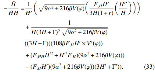
-\dfrac{\ddot{H}}{\dot{H}H} to identify some new parameters in further calculations. We begin by looking at the second derivative of H, i.e.,\ddot{H} = \dfrac{\mathrm{d}}{\mathrm{d}t}(H'\dot{\varphi}) . By expanding the derivative in this expression, we get\ddot{H} = \dot{\varphi}^{2}H''+\ddot{\varphi}H'.
(32) We first determine the value of
\ddot{\varphi} to get the solution of Eq. (32). We have done this by differentiating Eq. (25) with respect to t, which results in\begin{aligned}[b]\ddot{\varphi} =& -\frac{\dot{\varphi}}{(3H+\Gamma)^2(\sqrt{9\alpha^{2}+216\beta V(\varphi)})}((3H\\&+\Gamma)((108\beta F_{,H}H'V'(\varphi))+(F_{,HH}H'^{2}+H''F_{,H})(9\alpha^{2}\\&+216\beta V(\varphi)))- F_{,H}H'(9\alpha^{2}+216\beta V(\varphi))(3H'+\Gamma')). \end{aligned}
This allows us to obtain
\begin{aligned}[b]-\dfrac{\ddot{H}}{\dot{H}H} = &\dfrac{1}{H'}\bigg(\sqrt{9\alpha^{2}+216\beta V(\varphi)}\bigg(\dfrac{F_{,H}H'}{3H(1+r)}\bigg(\dfrac{H''}{H}\bigg)\bigg)\bigg)\\&+\dfrac{1}{H(3H+\Gamma)^{2}\sqrt{9\alpha^{2}+216\beta V(\varphi)}}\\&((3H+\Gamma)((108\beta F_{,H}H' \times V'(\varphi)) \\&+(F_{,HH}H'^{2}+H''F_{,H})(9\alpha^{2}+216\beta V(\varphi)))\\&-(F_{,H}H')(9\alpha^{2}+216\beta V(\varphi))(3H'+\Gamma')). \end{aligned}
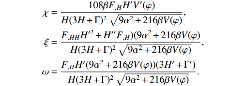
(33) We may rewrite this in a simple way by defining some parameters:
\nonumber -\frac{\ddot{H}}{\dot{H}H} = \frac{\eta}{H'}+(3H+\Gamma)(\chi+\xi)-\omega,
where the parameters are
\begin{aligned}[b] \chi &= \dfrac{108\beta F_{,H}H'V'(\varphi)}{H(3H+\Gamma)^{2}\sqrt{9\alpha^{2}+216\beta V(\varphi)}},\\ \xi &= \dfrac{F_{,HH}H'^{2}+H''F_{,H})(9\alpha^{2}+216\beta V(\varphi)}{H(3H+\Gamma)^{2}\sqrt{9\alpha^{2}+216\beta V(\varphi)}},\\ \omega &= \dfrac{F_{,H}H'(9\alpha^{2}+216\beta V(\varphi))(3H'+\Gamma')}{H(3H+\Gamma)^{2}\sqrt{9\alpha^{2}+216\beta V(\varphi)}}. \end{aligned}
-
The general formula for calculating the amplitude of adiabatic perturbations is given by [76]
P_{s}(k) = \frac{4}{25}\bigg(\frac{H}{|\dot{\varphi}|}\bigg)^{2}\mathrm{d}\varphi^2,
(34) where
\dot{\varphi} is given in Eq. (25). This equation is valid for a combination of inflation and radiation fields in the quasi-static phase of radiation production. Additionally, it can be shown that, in the quasi-static limit, and using an equation of state, this result holds true for any scalar field that is interacting adiabatically with another field. -
In this case, the term
\mathrm{d}\varphi^{2} is defined as follows:\mathrm{d}\varphi^2 = \frac{k_{F}T}{2\pi},
(35) with "freeze out number"
k_{F} = \sqrt{\Gamma H} . Inserting the value of T from Eq. (27) and using expression of ϵ in Eq. (29), we get the following expression ofP_{s}(k) for our model:P_{s}(k) = \frac{2}{25\pi}\bigg(\frac{3r}{4\alpha}\bigg)^{{1}/{4}}\bigg(\frac{H'}{\epsilon}\bigg)^{{3}/{2}} \bigg(\frac{\Gamma}{H}\bigg)^{{1}/{2}}.
(36) The spectral index specifies the relationship between the curvature perturbations and SR parameters. We calculate the scalar spectral index
n_{s} for our model asn_{s} = 1+\frac{\mathrm{d}\ln P_{s}(k)}{\mathrm{d}\ln k} = 1+\frac{\dot{\varphi}}{2H}\bigg(-\frac{H'}{H}+\frac{\Gamma'}{\Gamma}-\frac{3\epsilon'}{\epsilon}+\frac{3H''}{H'}\bigg).
(37) The following is the definition of the tensor power spectrum:
P_{T}(k) = \frac{32}{75m^{4}_{p}}V(\varphi) = \frac{32}{75m^{4}_{p}}\bigg(\frac{\Gamma^{2}((108\beta F+3\alpha^{2})^{2}-9\alpha^{2})}{23328\beta^{2}(F_{,H}H')^{2}+216\beta\Gamma^{2}}\bigg).
(38) Finally, the general expression for tensor-to-scalar ratio under the high-dissipative regime is calculated as
r = \frac{P_{T}(k)}{P_{s}(k)} = \frac{16\pi (4\alpha)^{{1}/{4}} V(\varphi)}{3m^{4}_{p}}(\Gamma^{-{3}/{4}}H^{{3}/{4}}\epsilon^{{3}/{2}}H'^{-{3}/{2}}).
(39) Next, we will present similar calculations for the low-dissipative regime.
-
In a low-dissipative regime, Eq. (34) is used to represent the amplitude of the scalar spectrum, but the term
\mathrm{d}\varphi is specified differently as\mathrm{d}\varphi = HT . Here,P_{s}(k) takes the following form:P_{s}(k) = \frac{4}{25}\bigg(\frac{T^{2}H'^{2}}{\epsilon^{2}}\bigg).
(40) Furthermore, it can be written as
P_{s}(k) = \bigg(\bigg(\frac{4}{625\alpha}\bigg)\epsilon^{-2}H'^{2}\Gamma H^{3}\bigg)^{{1}/{2}}.
(41) We analyze
n_{s} and r for low-dissipation asn_{s} = 1+\frac{\dot{\varphi}}{H}\bigg(\frac{3H'}{2H}+\frac{\Gamma'}{2\Gamma}-\frac{\epsilon'}{\epsilon}+\frac{H''}{H'}\bigg),
(42) r = \frac{P_{T}(k)}{P_{s}(k)} = \frac{16V(\varphi)}{3m^{4}_{p}}\bigg(\frac{\epsilon^{-2}H^{3}H'^{2}\Gamma }{\alpha}\bigg)^{{1}/{2}}.
(43) We have just completed the theoretical groundwork for our approach. Next, we will apply it to modified universe models with TE, RE, and BHDE (Secs. V, VI, and VII, respectively).
-
Tsallis entropy was introduced by Brazilian physicist Constantino Tsallis in
1988 [77]. This entropy is a generalization of the standard Boltzmann-Gibbs entropy, which is commonly used to discuss inflationary cosmology. This allows for the description of systems that exhibit non-Gaussian statistics, long-range correlations, and non-extensive behavior, which may be relevant to WI scenarios. It has been shown to be useful in describing dissipative systems, which is an essential feature of WI models. In WI, dissipation is introduced by considering the inflation field to be in contact with a thermal bath, which leads to non-conserved energy systems and results in the production of particles. Tsallis entropy can provide a more accurate description of the non-equilibrium dynamics of the inflation field and the thermal bath, paving a path to more accurate predictions for the inflationary observables. Tsallis entropy in WI models can lead to new and interesting results that cannot be obtained by using the standard Boltzmann-Gibbs entropy. It has been shown that TE can lead to power-law inflationary potentials, which has some interesting cosmological implications. Tsallis entropy in the WI mechanism is an important and active area of research, which has the potential to lead to new insights into the dynamics of the early universe and the generation of the cosmic structure. We have considered the Hubble horizon as a candidate for the IR-cutoff as the cosmic horizon for this entropy, which is{\cal{L}} = 1/H . The radius of the Hubble horizon [78] is considered asr_A = 1/\sqrt{H^{2}+K/a^{2}} ; as we are working in flat geometry, the curvature parameterK = 0 leads tor_A = {\cal{L}} . The Hawking temperature [79] defined by the surface gravity is taken to beT_{A} = 1/2\pi r_{A} ; by considering the radius, it turns out to beT_{A} = H/2\pi , where A is the area of the horizon. The volume is considered asV_A = (4/3)\pi R_{A}^{3} , which will becomeV_A = 4\pi/3H^{3} .The usual Friedmann equation is written as
F(H) = H^2 = \frac{8\pi}{3m^{2}_{p}}\rho.
(44) Here,
c = h = 1 , andm^{2}_{p} is the reduced Planck mass. ρ is the energy density of the fluid. Black hole entropy has received significant attention recently, particularly due to developments from Tsallis and Cirto [80]. They argued that the thermodynamic entropy of a black hole has a microscopic mathematical formulation that deviates from the area law, which is characterized asS = \gamma A^{\kappa},
(45) where γ is an unknown constant, A is the black hole horizon area, and κ is the Tsallis parameter, a real parameter that quantifies the degree of non-extensivity. In Ref. [81], a modified Friedmann equation was successfully developed, integrating modifications to Padmanabhan's Emergent Gravity proposal [82] by considering Tsallis-type entropy for the apparent horizon of an FLRW universe. The relevant Friedmann equation is [81]
(H^{2})^{2-\kappa} = \frac{8\pi}{3m^{2}_{p}}\rho.
(46) The following equation corresponds to the modified Friedmann universe with TE using the above equation:
F(H) = H^{2(2-k)}.
(47) By keeping in view, the original
F(H) in Eq. (23) turns out to beF(H) = \bigg(\frac{-3\alpha\pm\sqrt{9\alpha^{2}+216\beta V(\varphi)}}{108\beta}\bigg)^{(2-k)}.
(48) In our approach, H and Γ will be treated as a function of φ. These terms are chosen as the power-law functions of inflaton, which are defined as
\begin{array}{l} H(\varphi) = H_{0}\varphi^{n},\quad \Gamma(\varphi) = \Gamma_{0}\varphi^{m}, \end{array}
(49) where
H_{0} and\Gamma_{0} represent arbitrary constants, while the exponents n and m are not specified at present. We are going to count on Planck data to determine the power laws applicable to the underlying model. Using the TE given in Eq. (47), we evaluate the spectral indexn_s and tensor-to-scalar ratio r for a high-dissipative regime as\begin{aligned}[b]\\ n_{s} =& 1+(3 H_{0}^{4-2k} n^2 \varphi ^{n(4-2k)-1} (k-2))(\Gamma_{0}^2H_{0}^{4 k}\varphi^{2(m+2nk+2)}+432 \beta H_{0}^{10}n^4\varphi^{10 n}(k-2)^2)^{\tfrac{3}{2}}(m-3+2n+3((36 \beta \\&\times \Gamma_{0}^2 H_{0}^{4(1+k)}\varphi ^{2(m+2n+2nk+2)}(4(k-2) n+m+3)+\alpha ^2 \Gamma_{0}^2H_{0}^{6 k}\varphi^{2( m+3nk+2)} (2 (k-2) n+m+3))+(15552\beta^2H_{0}^{14}\\ &\times n^4 (k-2)^2 ((2 k-3) n+1) \varphi ^{14 n} + 432 \alpha ^2 \beta H_{0}^{2(5+k)} (k-2)^2 n^4 (n+1) \varphi ^{2n(5+k)}))), \end{aligned} (50) \begin{aligned}[b] r =& -(8\pi n^3(\varphi ^m)^{\tfrac{3}{2}} \sqrt{H_{0} \varphi ^n}((3 \alpha ^2+108 \beta (H_{0} \varphi ^n)^{4-2 k})^2-9 \alpha ^2)(H_{0}^{2(2-k)} (k-2) \varphi ^{-m+4n-2kn-3})^{\tfrac{3}{2}} (( \varphi ^{2 m+4}\Gamma_{0}^2\\& \times (36 \beta H_{0}^4 \varphi ^{4 n}+\alpha ^2(H_{0}\varphi^n)^{2k})^2)(\Gamma_{0}^2H_{0} ^{4 k}\varphi ^{2(m+2kn+2)}+432 \beta H_{0}^{10}n^4 \varphi ^{10 n}(k-2)^2))^{-\frac{3}{4}})(9\sqrt{3}H_{0}^{\tfrac{5}{4}}\varphi^{\tfrac{1}{4}(5n+m-6)}\\& \times \beta m_p^4(\Gamma_{0}\alpha^{-1} )^{\tfrac{1}{4}}(\Gamma_{0}^2 \varphi ^{2 m}+432 \beta H_{0}^{2(5-2k)}n^4\varphi ^{2(5n-2kn-2)}(k-2)^2))^{-1}. \end{aligned}
(51) Also, for the low-dissipative regime,
\begin{aligned}[b] n_{s} =& 1+ (36 \beta H_{0}^4 \varphi ^{4 n}+\alpha ^2 (H_{0} \varphi ^n)^{2 k})^{-1}(48 \beta H_{0}^8 n^4 \varphi ^{8 n} (k-2)^2 +\varphi ^4 (H_{0} \varphi ^n)^{4 k})^{-\tfrac{3}{2}} (1728 \beta ^2 H_{0}^{12} n^4 \varphi ^{12n-2} (k-2)^2 \\ & \times (m+(4 k -1) n)+1728 \alpha ^2 \beta^{2} H_{0}^{12+6k}n^4 \varphi ^{6n(2+k)+4}(k-2)^2 (m+7 n)(m+4+(8 k-9) n)+\alpha ^2 \varphi^4 (m+4 \\ & + (4k-1)n)(H_{0}\varphi^n)^{6k})(H_{0}^{3-2k}n^2 \varphi ^{n(3-2k)+1}(k-2)(36\beta H_{0}^4 \varphi ^{4 n}+\alpha ^2 \left(H_{0} \varphi^n\right)^{2k})), \end{aligned}
(52) r = \dfrac{4\alpha^{\tfrac{1}{2}} n^{2}\varphi^{4}(k-2)(H_{0}\varphi^{n})^{4k}(-9\alpha^{2}+(3\alpha^{2} +108\beta(H_{0}\varphi^{n})^{4-2k})^{2})(36H_{0}^{4}\beta\varphi^{4n}+\alpha^{2}(H_{0}\varphi^{n})^{2k})} {81\beta(\Gamma_{0}\varphi^{m}(H_{0}\varphi^{n})^{-1+4k})^{\tfrac{1}{2}} (48H_{0}^{8}(-2+k)^{2}n^{4}\beta\varphi^{8n}+\varphi^{4}(H_{0}\varphi^{n})^{4k})^{\tfrac{3}{2}} m_{p}^{4}}.
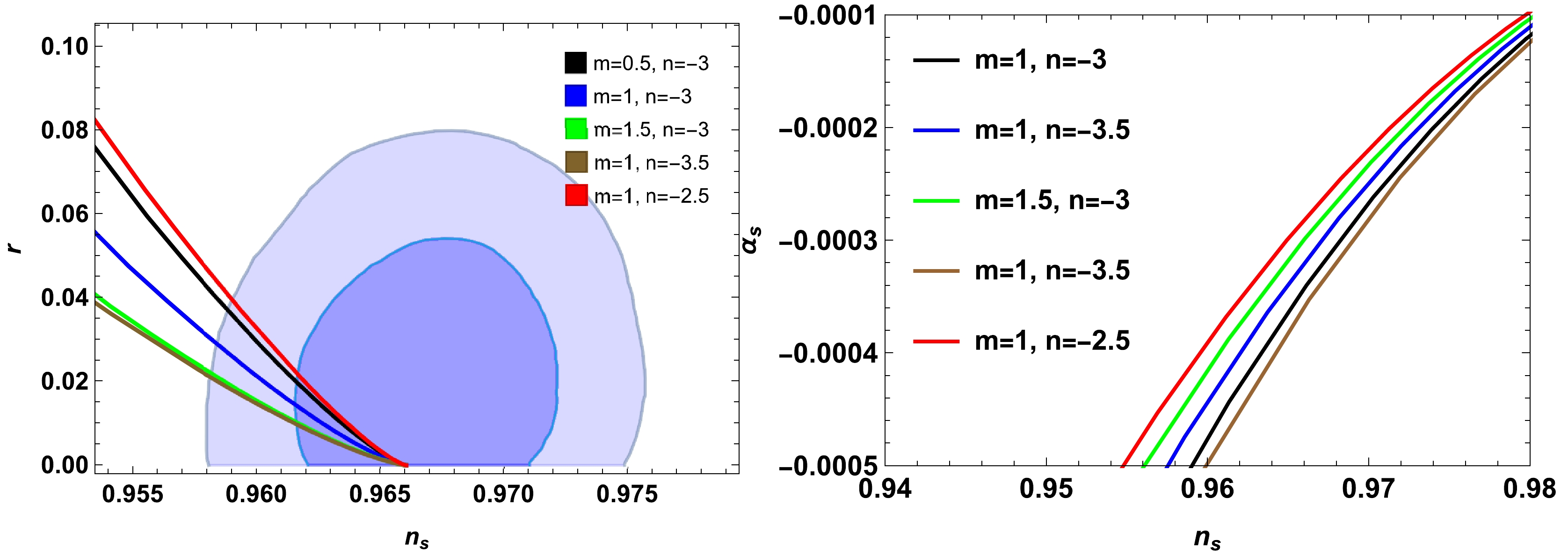
(53) The aforementioned information provides a theoretical foundation for inflation. Recent observational data from the Planck satellite also provide insightful information on the WI paradigm. They provide specific information about the spectral index and its variation. Figures 1 and 2 show that the constructed model incorporating WI using TE fitted well with the deep
2\sigma level of the Planck 2018 data [6, 7]. -
The concept of RE was introduced by Hungarian mathematician Alfred Renyi in
1960 [28]. Renyi entropy is a concept from information theory that is used in various fields, including physics and cosmology. It can be used to quantify the degree of entanglement between the inflaton field and its environment. During WI, the inflaton field is in contact with a thermal environment, which means that the inflaton field is not in a pure state. Instead, it is described by a density matrix that includes contributions from the thermal environment. The RE is a measure of the entanglement between the inflaton field and the environment and is defined as\nonumber S_{q} = \frac{1}{(1-q)}\ln(\mathrm{tr}(\rho^q)),
where ρ is the density matrix, and q is a parameter that determines the order of the entropy. When
q = 1 , Renyi entropy reduces to non-Neumann entropy, a standard entanglement measure. Renyi entropy has been used to study the dynamics of the inflaton field and its interaction with the thermal environment. It can be used to quantify the degree of entanglement between the inflaton field and its environment, and it has been used to study the dynamics of the inflaton field and quantum-to-classical transition during WI. In more recent times, it has been claimed that BHES = {A}/{4} is actually Tsallis entropy that results inS = \ln(1+{\delta}A/4) for the Renyi entropy content of the system. The Hubble horizon is considered as the IR cut-off.Renyi HDE can be defined as [83]
F(H) = \frac{3C^{2}H^{2}}{8\pi\left(1+\dfrac{\pi\delta}{H^{2}}\right)},
(54) which can be simplified as
F(H) = \frac{3C^{2}H^{4}}{8\pi(H^{2}+\pi\delta)}.
(55) Now, by using general
F(H) = H^2 given in Eq. (23), we get\begin{aligned}[b]F(H) =& \frac{3C^{2}}{8\pi}\bigg(\frac{-3\alpha\pm\sqrt{9\alpha^{2}+216\beta V(\varphi)}}{108\beta}\bigg)^{2}\\&\bigg(\frac{-3\alpha\pm\sqrt{9\alpha^{2}+216\beta V(\varphi)}}{108\beta}+\pi\delta\bigg)^{-1}. \end{aligned}
(56) In this model, we use the same power-law functions of inflaton for parameters H and Γ. The parameters
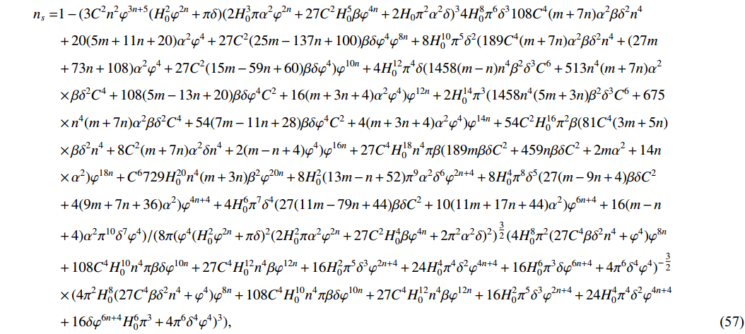
n_{s} and r for the low-dissipative regime are calculated as follow:\begin{aligned}[b] n_{s} =& 1-(3 C^2 n^2\varphi^{3n+5}(H_{0}^2 \varphi ^{2 n}+\pi \delta) (2 H_{0}^3 \pi \alpha ^2 \varphi ^{2 n}+27 C^2 H_{0}^5 \beta \varphi ^{4 n}+2 H_{0} \pi ^2 \alpha ^2 \delta )^3 4 H_{0}^8 \pi ^6 \delta ^3 108 C^4 (m+7 n) \alpha ^2 \beta \delta ^2 n^4\\ & + 20 (5 m+11 n+20) \alpha ^2 \varphi ^4+27 C^2 (25 m-137 n+100) \beta \delta \varphi ^4 \varphi ^{8 n}+8 H_{0}^{10} \pi ^5 \delta ^2 (189 C^4 (m+7 n) \alpha ^2 \beta \delta ^2 n^4+ (27 m\\ & + 73n+108) \alpha ^2 \varphi ^4+27 C^2 (15 m-59 n+60) \beta \delta \varphi ^4)\varphi ^{10 n}+4 H_{0}^{12} \pi ^4 \delta(1458 (m-n) n^4 \beta ^2 \delta^3 C^6+513 n^4 (m+7 n) \alpha ^2\\ & \times \beta \delta ^2 C^4+108 (5 m-13 n+20) \beta \delta \varphi ^4 C^2+16 (m+3 n+4) \alpha ^2 \varphi ^4)\varphi ^{12 n}+2 H_{0}^{14} \pi ^3(1458 n^4 (5 m+3 n) \beta ^2 \delta ^3 C^6+675 \\ & \times n^4 (m+7 n) \alpha ^2 \beta \delta ^2 C^4+54 (7 m-11 n+28) \beta \delta \varphi ^4 C^2+4 (m+3 n+4) \alpha ^2 \varphi ^4)\varphi^{14 n}+54 C^2 H_{0}^{16} \pi ^2 \beta (81 C^4 (3 m+5 n)\\ &\times \beta \delta ^2 n^4 +8 C^2 (m+7 n) \alpha ^2 \delta n^4+2 (m-n+4) \varphi ^4)\varphi ^{16 n}+27 C^4 H_{0}^{18} n^4 \pi \beta(189 m \beta \delta C^2+459 n \beta \delta C^2+ 2 m \alpha ^2+14 n \\\ & \times \alpha ^2) \varphi ^{18 n}+C^6 729 H_{0}^{20} n^4 (m+3 n) \beta ^2 \varphi ^{20 n}+8 H_{0}^2 (13 m-n+52) \pi ^9 \alpha ^2 \delta ^6 \varphi ^{2 n+4}+8 H_{0}^4 \pi ^8 \delta ^5(27 (m-9 n+ 4) \beta \delta C^2 \\ & + 4 (9m+7n+ 36) \alpha ^2)\varphi ^{4 n+4}+4 H_{0}^6 \pi ^7 \delta ^4(27 (11 m-79 n+44) \beta \delta C^2+10 (11 m+17 n+44) \alpha ^2) \varphi ^{6 n+4}+16 (m-n \\ & + 4) \alpha ^2 \pi ^{10}\delta ^7 \varphi^4) /(8 \pi(\varphi ^4 (H_{0}^2 \varphi ^{2 n}+\pi \delta)^2 (2 H_{0}^2 \pi \alpha ^2 \varphi ^{2 n}+ 27 C^2 H_{0}^4 \beta \varphi ^{4 n}+2 \pi ^2 \alpha ^2 \delta )^2)^{\tfrac{3}{2}}(4 H_{0}^8 \pi ^2 (27 C^4 \beta \delta ^2 n^4 + \varphi ^4) \varphi ^{8 n} \\ & + 108 C^4 H_{0}^{10} n^4 \pi \beta \delta \varphi ^{10 n} + 27 C^4 H_{0}^{12} n^4 \beta \varphi ^{12 n}+16 H_{0}^2 \pi ^5 \delta ^3 \varphi ^{2 n+4}+24 H_{0}^4 \pi ^4 \delta ^2 \varphi ^{4 n+4}+16 H_{0}^6 \pi ^3 \delta \varphi ^{6 n+4} + 4 \pi ^6 \delta ^4\varphi^4)^{-\tfrac{3}{2}} \\ &\times (4\pi ^2 H_{0}^8 (27 C^4 \beta \delta ^2 n^4 + \varphi ^4) \varphi ^{8 n} + 108 C^4 H_{0}^{10} n^4 \pi \beta \delta \varphi ^{10 n}+27 C^4 H_{0}^{12} n^4 \beta \varphi ^{12 n}+16 H_{0}^2 \pi ^5 \delta ^3 \varphi ^{2 n+4} +24 H_{0}^4 \pi ^4 \delta ^2 \varphi ^{4 n+4} \\ & + 16\delta \varphi ^{6 n+4}H_{0}^6 \pi ^3 +4 \pi ^6 \delta ^4 \varphi ^4)^{3}), \end{aligned} (57) \begin{aligned}[b] r =& ((2 ((3 \alpha ^2+((81 \beta C^2 H_{0}^4 \varphi ^{4 n})/(2 \pi ^2 \delta +2 \pi H_{0}^2 \varphi ^{2 n})))^2-9 \alpha ^2))(27 \pi \beta m_p^4 ((27 \beta C^4 H_{0}^8 n^4 \varphi ^{8 n-4} (2 \pi \delta +H_{0}^2 \varphi ^{2 n})^2/\pi ^2 (\pi \delta \\ & + H_{0}^2 \varphi ^{2n})^4)+4))^{-1})( \alpha C^4 H_{0} n^4 (2 \pi \delta +H_{0}^2 \varphi ^{2 n})^2(2 \pi ^2 \alpha ^2 \delta +27 C^2 \beta H_{0}^4 \varphi ^{4 n}+2 \pi \alpha ^2H_{0}^2\varphi^{2n})^{2})^{\frac{1}{2}}(\Gamma_{0} \varphi ^{m-n} (\pi \delta + \varphi ^{2 n} \\ &\times H_{0}^2)^2 (27 \beta C^4 H_{0}^{12} n^4 \varphi ^{12 n}+108 \pi \beta C^4 \delta H_{0}^{10} n^4 \varphi ^{10 n}+4 \pi ^2 H_{0}^8 \varphi ^{8 n} (27 \beta C^4 \delta ^2 n^4+\varphi ^4) + 4 \pi ^6 \delta ^4 \varphi ^4+16 \pi ^3 \delta H_{0}^6 \varphi ^{6 n+4} \\& + 24 \pi ^4 \delta ^2 H_{0}^4 \varphi ^{4 n+4}+16 \pi ^5 \delta ^3 H_{0}^2 \varphi ^{2 n+4}))^{-\frac{1}{2}}. \end{aligned}
(58) Under the high-dissipative regime,
n_{s} and r will have the following form:\begin{aligned}[b] n_{s} =& 1-9 C^2 H_{0}^4 n^2 \varphi ^{-m+4 n-3} (2 \pi \delta +H_{0}^2 \varphi ^{2 n})(1/8 \pi) (\pi \delta +H_{0}^2 \varphi ^{2 n})^{-2}( \varphi ^{m+2} (\pi \delta +H_{0}^2 \varphi ^{2 n}) (2 \pi ^2 \alpha ^2 \delta +27 \beta C^2 H_{0}^4 \varphi ^{4 n}\\ & + 2\pi \alpha ^2 H_{0}^2 \varphi ^{2 n}))(243 \beta C^4 H_{0}^{10} n^4 \varphi ^{10 n} (2 \pi \delta +H_{0}^2 \varphi ^{2 n})^2+4 \pi ^2 \Gamma_{0}^2 \varphi ^{2 m+4} (\pi \delta +H_{0}^2 \varphi^{2n})^4)^{-\tfrac{3}{2}}((\pi \delta +H_{0}^2 \phi ^{2 n})(2 \pi ^2 \alpha ^2 \delta \\ & + 27 \beta C^2 H_{0}^{4} \phi ^{4 n}+2 \pi \alpha ^2 H_{0}^{2} \phi ^{2 n}) ((12 H_{0}^2 n \varphi ^{2 n})(\pi \delta +H_{0}^2 \varphi ^{2 n})^{-1}-(6 H_{0}^2 n \varphi ^{2 n})(2 \pi \delta +H_{0}^2 \varphi ^{2 n})^{-1}+3 (m-4 n+3) \\ & + m+3 (n-1)-n) - 81 \beta C^2 n \varphi ^{4 n}(8 \pi ^2 \Gamma_{0}^2 \varphi ^{2 m+4} (2 \pi \delta +H_{0}^2 \varphi ^{2 n}) (H_{0}^3 \varphi ^{2 n}+\pi \delta H_{0})^4+ (18 \pi \alpha ^2 C^2 H_{0}^{10} n^3 \varphi ^{6 n} \\& \times (2 \pi ^2 \delta ^2 + H_{0}^4 \varphi ^{4 n}+3 \pi \delta H_{0}^2 \varphi ^{2 n}) (H_{0}^4 (m-3 n+2) \varphi ^{4 n}+3 \pi \delta H_{0}^2 (m-3 n+2) \varphi ^{2 n} + 2 \pi ^2 \delta ^2 (m-5 n+2)))- (243 \\ & \times \beta C^4 H_{0}^{14} n^3 \varphi ^{10 n} (2 \pi \delta +H_{0}^2 \varphi ^{2 n}) (H_{0}^4 (-m +n-2) \varphi ^{4 n}+\pi \delta H_{0}^2 (-3 m+n-6) \varphi ^{2 n} - 2 \pi ^2 \delta ^2 (m-n+2)))) / ((\pi \\ & \times \delta +H_{0}^2 \varphi ^{2 n})( 2 \pi ^2 \alpha ^2 \delta +27 \beta C^2 H_{0}^4 \varphi ^{4 n}+2 \pi \alpha ^2 H_{0}^2 \varphi ^{2 n} ) ((\pi \delta +H_{0}^2 \varphi ^{2 n}) (2 \pi ^2 \alpha ^2 \delta +27 \beta C^2 H_{0}^4 \varphi ^{4 n} + 2 \pi \alpha ^2 H_{0}^2 \varphi ^{2 n}) \\ & \times (243 \beta C^4 H_{0}^{10} n^4 \varphi ^{10 n} (2 \pi \delta +H_{0}^2 \varphi ^{2 n})^2+4 \pi ^2 \Gamma_{0}^2 \varphi ^{2 m+4} (\pi \delta +H_{0}^2 \varphi ^{2 n})^4)))), \end{aligned}
(59) \begin{aligned}[b] r =& ((2\pi^{-1}H_{0} \varphi ^n)^{\tfrac{1}{2}} (\varphi ^m)^{3/2} ((3 \alpha ^2+81 \beta C^2 H_{0}^4 \varphi ^{4 n}(2 \pi ^2 \delta +2 \pi H_{0}^2 \varphi ^{2 n})^{-1})^2-9 \alpha ^2)(3 \beta m_p^4 (H_{0} n \varphi ^{n-1})^{3/2} (\Gamma_{0} \varphi ^{m-n}( H_{0} \\& \times \alpha)^{-1})^{\tfrac{1}{4}}(243 \beta C^4 H_{0}^{10} n^4 \varphi ^{10 n-4} (2 \pi \delta +H_{0}^2 \varphi ^{2 n})^2\pi ^{-2} (\pi \delta +H_{0}^2 \varphi ^{2 n})^{-4}+4 \Gamma_{0}^2 \varphi ^{2 m}))^{-1})( C^2 H_{0}^4 n^3 \varphi ^{-m+4 n-3} (2 \pi \delta +H_{0}^2 \\ &\times \varphi ^{2 n})(\pi \delta +H_{0}^2 \varphi ^{2 n})^{-2})^{\tfrac{3}{2}} ((\Gamma_{0}^2 \varphi ^{2 m+4} (\pi \delta +H_{0}^2 \varphi ^{2 n})^2 (2 \pi ^2 \alpha ^2 \delta +27 \beta C^2 H_{0}^4 \varphi ^{4 n}+2 \pi\alpha ^2 H_{0}^2 \varphi ^{2 n})^2)(243 \beta C^4 H_{0}^{10} n^4 \varphi ^{10 n}\\ &\times (2 \pi \delta + H_{0}^2 \varphi ^{2 n})^2 +4 \pi ^2 \Gamma_{0}^2 \varphi ^{2 m+4} (\pi \delta +H_{0}^2 \varphi ^{2 n})^4)^{-1})^{\tfrac{3}{4}}. \end{aligned}
(60) The consistency of the
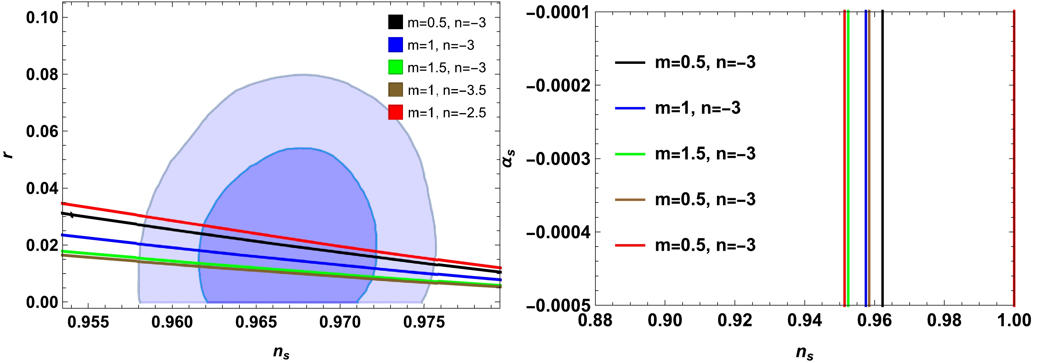
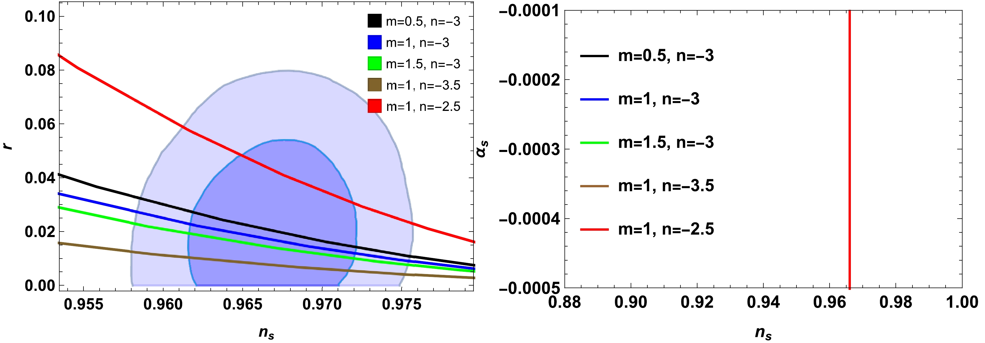
n_s-r trajectories with the Planck2018 data is shown in the left plots of Figs. 3 and 4, and then_s-\alpha_s trajectories are displayed in the right panels of Figs. 3 and 4. Both graphs fit well with current observational data up to the2\sigma level. -
Barrow recently proposed a fractal pattern for the black hole horizon, suggesting that the area of the horizon could increase due to quantum-gravitational deformation [84]. This modifies the area-law entropy, resulting in
S_{h}\sim A^{1+ \tfrac{\Delta}{2}} . The cosmological field equations based on Barrow's modified entropy were investigated in Ref. [85]. Subsequently, researchers have explored new developments in the literature to test the effectiveness of Barrow's entropy in the cosmological context [86]. In addition, the BHDE model was introduced in Ref. [87] and assessed against recent cosmological data in Ref. [88]. It was discovered that BHDE efficiently describes the late-time accelerating expansion of the universe and has the correct asymptotic behavior [89]. Notably, although Barrow's entropy shares similarities with TE, the origin and physical motivation of the two are distinct. Tsallis non-additive entropy correction is motivated by extending traditionalthermodynamics to a non-extensive one, while Barrow's correction to entropy is based on a complex fractal horizon structure caused by quantum gravitational effects, which was driven by the COVID-19 viral explanation. Hence, a deformed black hole entropy expression is given by [29]S_{B} = \bigg(\frac{A}{A_{0}}\bigg)^{\Delta+1},
(61) where the new term Δ is defined in the range
[0, 1] ,A_{0} is the Planck area, and A is the standard horizon area. Therefore, the goal of this modified entropy relation is simply to produce BHDE on the basis of HDE, whereby phenomenology is improved, and set it apart from the HDE standard framework. Barrow's entropy is defined as [86]F(H) = {\cal{C}}{\cal{L}}^{-2(1-\Delta)},
(62) where
{\cal{C}} = 3c^{2}M^{2}_{p} ,M_{p} is the Planck mass,c^{2} is a dimensionless constant, and{\cal{L}} represents the IR cutoff, which is taken to be the Hubble horizon{\cal{L}} = 1/H . Parameter{\cal{C}} has dimension[{\cal{L}}]^{-2(1-\Delta)} . For vanishing Δ, Eq. (62) will be the standard HDE, and it becomes constant under the limit\Delta\rightarrow1 . Our model now takes the following form:F(H) = {\cal{C}}\bigg(\frac{1}{H}\bigg)^{-2(1-\Delta)}.
(63) Using Eq. (23), we get
F(H) = {\cal{C}}\bigg(\frac{-3\alpha\pm\sqrt{9\alpha^{2}+216\beta V(\varphi)}}{108\beta}\bigg)^{(1-\Delta)}.
(64) In this model, we followed similar expressions of H and Γ to those used in the previous two models. The parameters
n_{s} and r for the low-dissipative regime are calculated as\begin{aligned}[b] n_{s} =& 1+(c (\Delta -1) n^2 (\varphi ^{n}H_{0})^{-2 (\Delta -1)}\varphi)(\alpha ^2+36 \beta c (\varphi ^{n}H_{0})^{-2 (\Delta -1)})(48\beta c^2H_{0}^{4(1-\Delta)}n^4\varphi^{4n(1-\Delta)}(\Delta -1)^2+\varphi ^4)^{-\frac{1}{2}}\\ & \times (m+2 (n-1)+3n+(2(\alpha^{4}(48 \beta c^2 H_{0}^{4(1-\Delta)}\varphi ^{4n(1-\Delta)}n^4(n+1)(\Delta - 1)^2+\varphi ^4 ((2 \Delta -1) n+3)) +(72 \alpha ^2\beta c (\varphi ^{n}\\& \times H_{0})^{-2 (\Delta -1)}(48 \beta c^2H_{0}^{4(1-\Delta)}n^4\varphi ^{4n(1-\Delta)}(\Delta-1)^2(\Delta n+1)+\varphi ^4 ((3 \Delta -2) n+3))) +(1296 \beta ^2 c^2 H_{0}^{4(1-\Delta)}\varphi ^{4n(1-\Delta)}\\ & \times (48 \beta c^2n^4 (\Delta-1)^2 H_{0}^{4(1-\Delta)}\varphi^{4n(1-\Delta)}((2\Delta -1)n+1)+\varphi ^4 ((4 \Delta -3) n+3))))((48 \beta c^2H_{0}^{4(1-\Delta)} n^4 \varphi^{4n(1-\Delta)}(\Delta -1)^2\\& + \varphi ^4)(\alpha ^2+36 \beta c(\varphi ^{n}H_{0})^{-2 (\Delta -1)})^2)^{-1})), \end{aligned} (65) \begin{aligned}[b] r = &4 \varphi ^4 \alpha^{\tfrac{1}{2}}n^2 c ((3 \alpha ^2+108 \beta c (\varphi ^{n}H_{0})^{-2 (\Delta -1)})^2-9 \alpha ^2) (\Delta -1) (\alpha ^2+36 \beta c(\varphi ^{n}H_{0})^{-2 (\Delta -1)}) (81 \beta m_p^4 (48 \beta c^2 H_{0}^{4(1-\Delta)} \\ &\times n^4\varphi ^{4n(1-\Delta)}(\Delta -1)^2+\varphi ^4))^{-1} (\Gamma_{0} H_{0}^{3+4\Delta} \varphi^{m+3n+4n\Delta}(48 \beta c^2 H_{0}^{4(1-\Delta)} n^4 \varphi^{4n(1-\Delta)}(\Delta -1)^2+\varphi ^4))^{-\tfrac{1}{2}}. \end{aligned}
(66) For the high-dissipative regime,
n_{s} and r are formed as\begin{aligned}[b]n_{s} =& 1+(3 c (\Delta -1) n^2 \varphi ^{-m-2}(\varphi ^{n}H_{0})^{-2(\Delta-1)})( \varphi ^{m+2} (\alpha ^2+36 \beta c (\varphi ^{n}H_{0})^{-2 (\Delta -1)})(432 \beta c^2 (\Delta -1)^2 H_{0}^6 n^4 \varphi ^{6 n}(\varphi ^{n}H_{0})^{-4 \Delta } \\& + \Gamma_{0}^2 \varphi ^{2 m+4})^{-\tfrac{1}{2}})(m\varphi^{-1}+3 (n-1)\varphi^{-1}- n\varphi^{-1}+(3(\Gamma_{0}^{2}\varphi^{4+2m}(36 \beta c (m+4 (\Delta -1) n+3) (\varphi ^{n}H_{0})^{-2 (\Delta -1)}+\alpha ^2 (m \\ & + 2(\Delta -1) n+3)) +(432 \beta c^2 (\Delta -1)^2 H_{0}^6 n^4 \varphi ^{6 n} (\varphi ^{n}H_{0})^{-4 \Delta }(36 \beta c ((2 \Delta -1) n+1) (\varphi ^{n}H_{0})^{-2 (\Delta -1)}+\alpha ^2 (n+1)))))/ \\ & \times (\varphi(\alpha ^2+36 \beta c (\varphi ^{n}H_{0})^{-2 (\Delta -1)})(432\beta c^2(\Delta -1)^2 H_{0}^6 n^4 \varphi ^{6 n} (\varphi ^{n}H_{0})^{-4\Delta}+\Gamma_{0}^2 \varphi ^{2 m+4}))), \end{aligned}
(67) \begin{aligned}[b] r =& (8\pi \varphi ^4 (\varphi ^m)^{\tfrac{3}{2}} \sqrt{H_{0} \varphi ^n}((3 \alpha ^2+108 \beta c(\varphi ^{n}H_{0})^{-2 (\Delta -1)})^2-9 \alpha ^2)(9 \sqrt{3} \beta m_p^4 (H_{0} n \varphi ^{n-1})^{3/2}(\Gamma_{0} \varphi ^{m-n}(\alpha H_{0})^{-1})^{\tfrac{1}{4}}(432 \\ & \times \beta c^2(\Delta -1)^2 H_{0}^6 n^4 \varphi ^{6 n}(\varphi ^{n}H_{0})^{-4 \Delta }+\Gamma_{0}^2 \varphi ^{2 m+4}))^{-1})(c (\Delta -1) n^3 \varphi ^{-m-3}(\varphi ^{n}H_{0})^{-2 (\Delta -1)}\Gamma_{0} \varphi ^{m+2}(\alpha ^2+36 \beta c(\varphi ^{n}\\ &\times H_{0})^{-2 (\Delta -1)}) (432 \beta c^2 (\Delta -1)^2 H_{0}^6 n^4 \varphi ^{6 n} (\varphi ^{n}H_{0})^{-4 \Delta }+\Gamma_{0}^2 \varphi ^{2 m+4})^{-\tfrac{1}{2}})^{\tfrac{3}{2}}. \end{aligned}
(68) The
n_s-r trajectories are consistent with Planck 2018 data, as shown in the left plots of Figs. 5 and 6. The consistency ofn_s-\alpha_s trajectories is displayed in the right panels of Figs. 5 and 6. It is found that the model is fitted with current observational data up to the2\sigma level.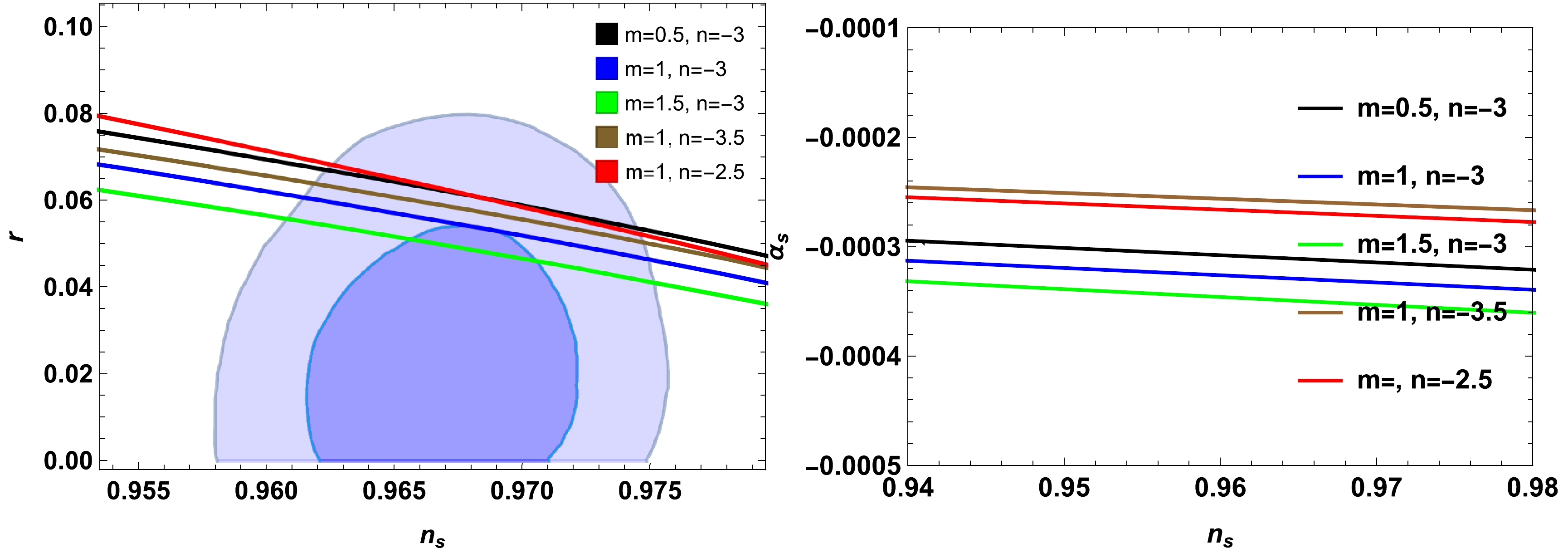
Figure 5. (color online) Left plot for
n_{s}-r plane and right plot forn_s-\alpha_s during low-dissipative regime within contours of Plank 2018 data for\bar{\lambda}=0.5, 1, 1.5 . Here, we fixedH_0=k=\kappa=1 ,\Gamma_0=0.5 ,m_p=1 ,\alpha=1 , and\gamma=0.16 .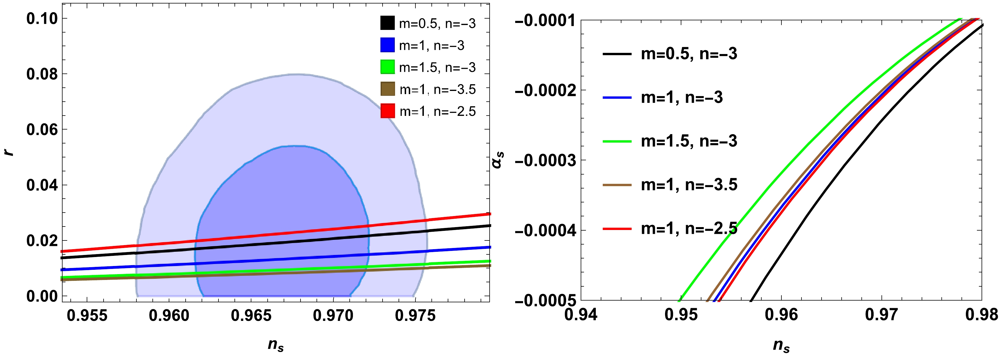
Figure 6. (color online) Left plot for
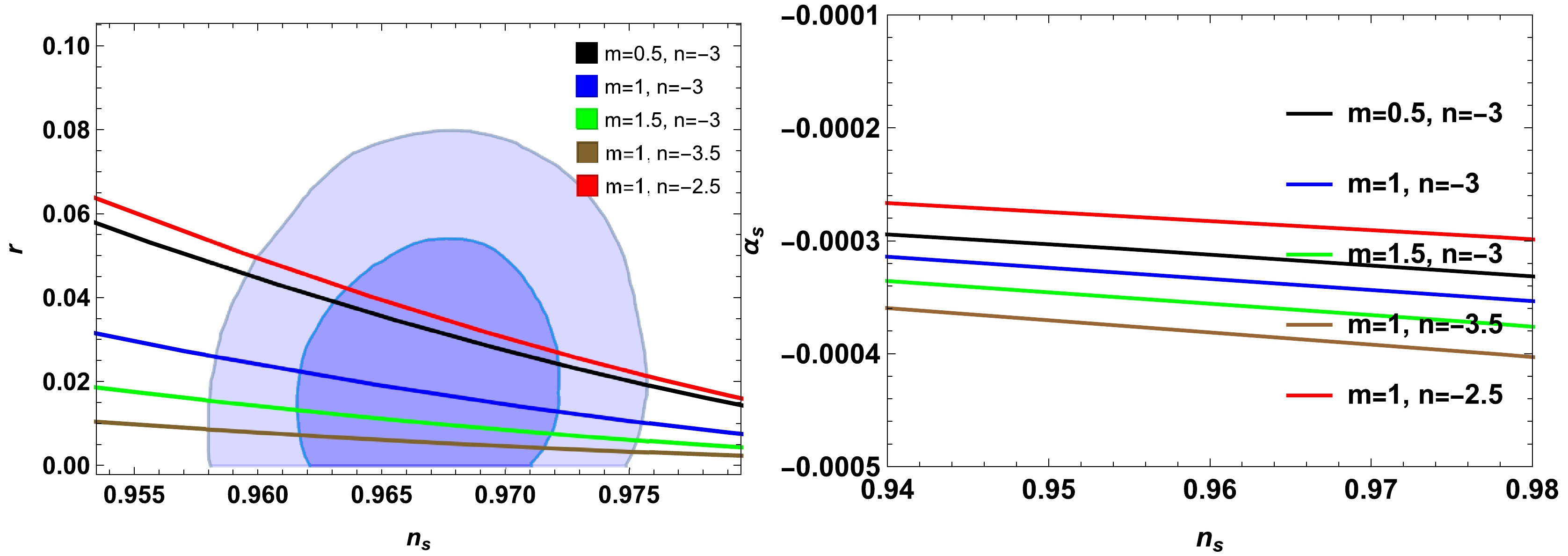
n_{s}-r plane and right plot forn_s-\alpha_s during high-dissipative regime within contours of Plank 2018 data by varyingm=0.5, 1, 1.5 andn=-3.5,-3,-2.5 . Here, we fixed\delta = 0.04,~c = 10^{45},\; \Gamma_0 = 0.5,\; H_0 = 1.5,\; \alpha = 1 ,\beta = 0.1 , andm_p=1 . -
Recently, there has been growing interest in studying the connection between early-time inflation and DE models. While there has been significant research to apply the holographic principle in late-time cosmology and the DE era, no attempts have been made to test it in the early universe to achieve an inflationary model with holographic origins. Such consideration holds the same importance as its well-established applications in late-time cosmology. In addition, the reduction of early horizons naturally results in an increase in holographic energy density during inflationary scales. In one study [35], the holographic origins of inflation were discovered by applying the holographic principle to the early cosmos. The analysis showed a perfect agreement between the theoretical predictions and Planck
2018 data, especially at the extremely precise1\sigma level. Saleem and Shahid [42] investigated the WI phenomenon in a modified cosmological model within Rastall gravity. They adopted Tsallis and BHDE entropies for the usual Friedmann equations. They computed SR parameters and inflationary observables for both extremes (low and high) of dissipation to compare the theoretical predictions of these models with current observational data. The free parameters were constrained by the Planck limits on inflationary trajectories. The results are interesting and physically viable up to the1\sigma level. Younas et al. [90], using some important entropies in the Chern-Simons modified gravity, discussed the DE models and several different involved model parameters regarding the evolution of the universe. Ghaffari et al. [91], using Sharma-Mittal entropy, examined some characteristics of Schwarzschild and Schwarzschild-de Sitter black holes. Jahromi et al. [92] considering a flat FRW universe and studied SMHDE analytically in the frame of the holographic principle. In [93], the authors showed that the generalization that unifies Rényi and Tsallis entropy in a coherent picture naturally comes into being through the q-formalism of generalized logarithm and exponential functions. Upadhyay and Dubey diagnosed the SMHDE model through the statefinder and checked the stability of the models under the allowed range of involved parameters [94]. In Ref. [95], Ayman studied a newf({\cal{T}}) modified gravity model using a Tsallis HDE model with a Hubble cutoff and confirmed that the growth of DE and the universe is in acceleration mode. Astashenok and Tepliakov presented the Tsallis HDE model with an event horizon cut-off in the framework of thef(R) theory of gravity [96]. In particular, they observed the cosmological evolution by consideringf(R) = R+\lambda R^2 -\sigma \mu/R and showed a sufficient accuracy of the model with SN Ia observational data for different values of involved model parameters.The authors of Ref. [97] considered the linear and quadratic perturbations for a scalar-tensor model with non-minimal coupling to curvature, coupling to the Gauss-Bonnet invariant, and non-minimal kinetic coupling to the Einstein tensor was developed. In this mechanism, they discussed the SR inflation in scalar-tensor models and found a consistency relation that is useful to discriminate the model from the standard inflation with canonical scalar field. The SR approximation of cosmic inflation within the context of
f(R,T) gravity was analyzed in [44], where the authors chose a minimal coupling between matter and gravity and obtained the modified SR parameters. They further concluded that the Starobinsky-like model predictions are in good agreement with the last Planck measurement. In the context of thef(T,{\cal{T}}) theory of gravity, researchers explored the concept of cosmological inflation with the assumptions of SR conditions and determined different observables related to inflation [98]. The SR inflationary models in a class of modified theories of gravity that contains non-minimal curvature-inflaton coupling, i.e.,f(R,T) gravity withRT mixing term, were analyzed in [99].Recently, Capozzielo and Shokri [62] discussed cosmic inflation in the framework of
f(Q) gravity. Motivated by the ideas of [42] and [62], our main objective is to successfully generate inflation driven by the relative energy densities of Barrow holographic, Renyi, and Tsallis inflation by examining their potential. We show that the natural simplicity of basic formalism displays high efficiency and yields inflationary observables that perfectly align with observational data. To do this, we incorporate TE, RE, and BHDE entropy and modify the Friedmann equations and continuity equation using a general Hubble parameter function within thef(Q) framework. By depictingn_{s}-r andn_{s}-\alpha_{s} trajectories, we have examined how well the underlying model fits the Planck2018 data. To obtain consistent findings, we imposed constraints on all significant model parameters.The results are explained as follows:
● Figures 1 and 2 show graphical representations of
n_{s}-r on the left siden_{s}-\alpha_{s} on the right side during low- and high-dissipative regimes. We found that the results lie within the range of Planck 2018 data. In Fig. 1, the allowed ranges for the free parameters m and n in left plot arem\in[-1,3] andn\in[-4,-1.5] , and the ranges for right plot arem\in[-1.5,6] andn\in[-9,-0.5] . In the left plot of Fig. 2,m\in[0.3,2] andn\in[-3.5,-2.5] , and in the right plot,m\in[0.47,1.57] andn\in[-3,-2.5] . Figures 1 and 2 show good agreement within the deep2\sigma level of Planck data.● For Renyi entropy, Figs. 3 and 4 have the same behavior as mentioned previously. The results are consistent with standard Planck data. In Fig. 3s, the ranges for the free parameters m and n in left plot are
m\in[-0.5,7] andn\in[-9,-2] and those in right plot arem\in[0.2,4] andn\in[-3.86,-1.9] . In Fig. 4, the allowed ranges of the free parameters for the left plot arem\in[-2,9] andn\in[-4,-1] and for the right plot arem\in[-8,5] andn\in[-9,-0.5] .● Figures 5 and 6 are plotted using BE. In Fig. 5, the allowed ranges for free parameters m and n in the left plot are
m\in[-0.5,4] andn\in[-4,-2] and in the right plot arem\in[0.5,2.5] andn\in[-5,-1.5] . In Fig. 6, the allowed ranges for the left plot arem\in[-1,4] andn\in[-8,-2] and for the right plot arem\in[-0.5,1.7] andn\in[-9,-1.5] . All these figures are consistent with Planck data up to the2\sigma level.The main task of this manuscript is to use different entropies in
f(Q) gravity, develop corresponding field equations, and discuss the phenomena of WI. From cosmological observations, the universe has experienced two phases of accelerated expansion, one at the early universe with exponential expansion and other at late times. To describe this behavior, modified gravitational theories can be constructed to provide an extra degree of freedom [100] or introduce new fields like the inflaton [101] or dark energy concept [102]. The first approach is to start from GR and add correction terms, resulting inf(R) gravity [103],f(G) gravity [104], orf(P) gravity [105], or to construct gravitational modifications using torsion, such asf(T) gravity [106], non-metricity gravity [69], or other geometrical structures.In Ref. [107], the authors studied WI using vector fields in the background of a locally rotationally symmetric Bianchi type I model of the universe and formulated the field equations, SR, and perturbation parameters under SR approximation. In this scenario, they showed that the graphical behavior of these parameters is compatible with WMAP
7 and the Planck observational data. Using the Bianchi type I universe model, the authors of Ref. [108] studied WI during the intermediate era. They calculated entropy density, scalar (tensor) power spectra, their corresponding spectral indices, tensor-scalar ratio, and running of spectral index in terms of inflaton and constrained these cosmological parameters with Planck2014 results and WMAP7 probe. The dynamics of WI were discussed in Ref. [109], where the authors explored the inflation driven by non-Abelian gauge fields using the Bianchi type I universe model.The impact of bulk viscous pressure on the warm inflationary modified Chaplygin gas model, in the context of the FRW universe, is discussed in Ref. [110], where the authors found that the viscous inflationary model remains compatible with the WMAP7 and Planck probe. The authors of Ref. [111] studied cosmic WI during rapid oscillations using the concept of non-minimal derivative coupling framework. They considered an anisotropic and homogeneous Bianchi I background, developed the formalism of anisotropic oscillatory inflation, and found some constraints for the existence of inflation. An early cosmic phenomenon inspired by inhomogeneous DE fluid models was studied in Ref.[112]. In particular, they determined viscosity through energy density and Hubble parameter, which act as corrections to a perfect DE fluid. Based on current analysis, we have observed that the DE models in the framework of modified theories of gravity provide some impressive results about the dynamics of WI. As minimizing the usage of exotic matter for the physical viability of cosmic dynamics is one of the primary goal of studies on the inflationary universe, it seems that
f(Q) is a good candidate to accomplish this. We hope our findings are fruitful for the scientific community. -
All data generated or analyzed during this study are included in this published article.


 Abstract
 HTML
HTML Reference
 Related
 PDF
PDF





 DownLoad:
