


 Abstract
 HTML
HTML Reference
 Related
 PDF
PDF


-
Cosmic inflation was proposed in the early 1980s and has become an essential component of modern cosmology. It provides a compelling mechanism to resolve the horizon and flatness problems of the Big Bang model and successfully explains the origin of primordial inhomogeneities that seed the large-scale structure of the universe [1, 2]. High-precision observations of the cosmic microwave background (CMB), most notably from the Planck satellite, have strongly supported the inflationary paradigm by tightly constraining key observables such as the scalar spectral index
$ n_s $ , the tensor-to-scalar ratio r, and the amplitude of primordial perturbations. Despite its observational success, inflation formulated within classical General Relativity (GR) is fundamentally incomplete in the past due to the presence of the Big Bang singularity, where physical quantities such as energy density and curvature diverge. This singularity obstructs a consistent description of the initial conditions of inflation and limits the predictive power of inflationary scenarios. Over the past two decades, loop quantum cosmology (LQC) has emerged as a well-motivated framework to address this limitation by incorporating quantum geometric effects inspired by loop quantum gravity (LQG). In LQC, the Big Bang singularity is generically resolved and replaced by a non-singular quantum bounce [3−5], providing a well-defined pre-inflationary history of the universe. LQC is constructed as a symmetry-reduced application of LQG using Ashtekar variables and Hamiltonian techniques [6−8]. Within this framework, quantum gravity effects become significant at energy densities approaching the Planck scale and modify the classical Friedmann dynamics. These modifications not only ensure the boundedness of physical observables but also naturally lead to a transition from a contracting pre-bounce phase to an expanding post-bounce universe. From an observational perspective, such pre-inflationary dynamics may influence the onset and duration of inflation and leave imprints on large-scale CMB observables.A key advantage of LQC in the context of Planck-era cosmology is its ability to provide well-defined initial conditions for inflation at the quantum bounce. In classical GR, all inflationary models are geodesically incomplete in the past, making the choice of initial conditions ambiguous [9, 10]. In contrast, LQC allows the inflaton field and its velocity to be specified unambiguously at the bounce, where the energy density reaches a universal maximum. The subsequent evolution can then be tested against observational requirements, most notably the requirement of sufficient slow-roll inflation. Current Planck constraints demand at least 60 e-folds of inflation, while some models predict significantly larger values [11]. Initial conditions that fail to produce adequate inflation can therefore be observationally excluded. An important implication of the quantum bounce is that the pre-inflationary phase may affect the dynamics of scalar perturbations and modify inflationary observables such as the scalar spectral index
$ n_s $ and the tensor-to-scalar ratio r. Consequently, LQC provides a natural arena to explore potential deviations from standard inflation that remain consistent with Planck data while offering insights into quantum gravity effects. Several approaches to cosmological perturbations in LQC have been developed, and recent studies have shown that the resulting predictions can be compatible with current observational bounds while still allowing for distinctive signatures at large scales.In this work, we study the background evolution of the universe in LQC for a mixed scalar-field potential, with particular emphasis on identifying the initial conditions of the inflaton field at the quantum bounce that lead to successful slow-roll inflation consistent with Planck observations. We focus on background dynamics and numerically analyze whether a sufficient number of e-folds can be achieved for various initial conditions at the bounce. For kinetic-energy-dominated (KED) initial conditions, the cosmic evolution naturally separates into three phases: the bouncing phase, a transition phase, and the slow-roll inflationary phase. In contrast, for potential-energy-dominated (PED) initial conditions, the bouncing and transition phases are absent, although slow-roll inflation may still occur. The dynamical behavior of the pre-inflationary and inflationary epochs has been extensively reviewed in Refs. [12−23]. The paper is organized as follows. In Sec. II, we present the effective background equations of LQC for a spatially flat Friedmann–Lemaître–Robertson–Walker (FLRW) universe. In Subsections II A and II B, we discuss inflationary parameters, analyze the numerical evolution of the Mixed Large-Field Inflation (MLFI) model, and examine whether it produces a viable slow-roll inflationary phase with at least 60 e-folds. Sec. III is devoted to a phase-space analysis, and our conclusions are summarized in Sec. IV.
-
Cosmic inflation was proposed in the early 1980s and has become an essential component of modern cosmology. It provides a compelling mechanism to resolve the horizon and flatness problems of the Big Bang model and successfully explains the origin of primordial inhomogeneities that seed the large-scale structure of the universe [1, 2]. High-precision observations of the cosmic microwave background (CMB), most notably from the Planck satellite, have strongly supported the inflationary paradigm by tightly constraining key observables such as the scalar spectral index
$ n_s $ , the tensor-to-scalar ratio r, and the amplitude of primordial perturbations. Despite its observational success, inflation formulated within classical General Relativity (GR) is fundamentally incomplete in the past due to the presence of the Big Bang singularity, where physical quantities such as energy density and curvature diverge. This singularity obstructs a consistent description of the initial conditions of inflation and limits the predictive power of inflationary scenarios. Over the past two decades, loop quantum cosmology (LQC) has emerged as a well-motivated framework to address this limitation by incorporating quantum geometric effects inspired by loop quantum gravity (LQG). In LQC, the Big Bang singularity is generically resolved and replaced by a non-singular quantum bounce [3−5], providing a well-defined pre-inflationary history of the universe. LQC is constructed as a symmetry-reduced application of LQG using Ashtekar variables and Hamiltonian techniques [6−8]. Within this framework, quantum gravity effects become significant at energy densities approaching the Planck scale and modify the classical Friedmann dynamics. These modifications not only ensure the boundedness of physical observables but also naturally lead to a transition from a contracting pre-bounce phase to an expanding post-bounce universe. From an observational perspective, such pre-inflationary dynamics may influence the onset and duration of inflation and leave imprints on large-scale CMB observables.A key advantage of LQC in the context of Planck-era cosmology is its ability to provide well-defined initial conditions for inflation at the quantum bounce. In classical GR, all inflationary models are geodesically incomplete in the past, making the choice of initial conditions ambiguous [9, 10]. In contrast, LQC allows the inflaton field and its velocity to be specified unambiguously at the bounce, where the energy density reaches a universal maximum. The subsequent evolution can then be tested against observational requirements, most notably the requirement of sufficient slow-roll inflation. Current Planck constraints demand at least 60 e-folds of inflation, while some models predict significantly larger values [11]. Initial conditions that fail to produce adequate inflation can therefore be observationally excluded. An important implication of the quantum bounce is that the pre-inflationary phase may affect the dynamics of scalar perturbations and modify inflationary observables such as the scalar spectral index
$ n_s $ and the tensor-to-scalar ratio r. Consequently, LQC provides a natural arena to explore potential deviations from standard inflation that remain consistent with Planck data while offering insights into quantum gravity effects. Several approaches to cosmological perturbations in LQC have been developed, and recent studies have shown that the resulting predictions can be compatible with current observational bounds while still allowing for distinctive signatures at large scales.In this work, we study the background evolution of the universe in LQC for a mixed scalar-field potential, with particular emphasis on identifying the initial conditions of the inflaton field at the quantum bounce that lead to successful slow-roll inflation consistent with Planck observations. We focus on background dynamics and numerically analyze whether a sufficient number of e-folds can be achieved for various initial conditions at the bounce. For kinetic-energy-dominated (KED) initial conditions, the cosmic evolution naturally separates into three phases: the bouncing phase, a transition phase, and the slow-roll inflationary phase. In contrast, for potential-energy-dominated (PED) initial conditions, the bouncing and transition phases are absent, although slow-roll inflation may still occur. The dynamical behavior of the pre-inflationary and inflationary epochs has been extensively reviewed in Refs. [12−23]. The paper is organized as follows. In Sec. II, we present the effective background equations of LQC for a spatially flat Friedmann–Lemaître–Robertson–Walker (FLRW) universe. In Subsections II.A and II.B, we discuss inflationary parameters, analyze the numerical evolution of the Mixed Large-Field Inflation (MLFI) model, and examine whether it produces a viable slow-roll inflationary phase with at least 60 e-folds. Sec. III is devoted to a phase-space analysis, and our conclusions are summarized in Sec. IV.
-
In this section, we briefly review the effective background dynamics of LQC and analyze the occurrence of a quantum bounce followed by slow-roll inflation for a mixed inflaton potential. We consider a spatially flat, homogeneous, and isotropic FLRW universe. In the effective description of LQC, the Hamiltonian is given by [7, 24]
$ {\cal{H}}=-\frac{3v\sin^2(\lambda b)}{8\pi G \gamma^2\lambda^2}+{\cal{H}}_M, $
(1) where
$ {\cal{H}}_M $ denotes the matter Hamiltonian and$ v=v_0 a^3 $ is the physical volume, with$ v_0 $ being the volume of the fiducial cell and a the scale factor. Here,$ G=1/m_{\rm{Pl}}^2 $ , with$ m_{\rm{Pl}} $ denoting the Planck mass. The Barbero–Immirzi parameter γ is fixed by black hole thermodynamics in LQG as$ \gamma\simeq 0.2375 $ [25, 26]. Hamilton's equations for the canonical variables v and b are$ \begin{aligned} \dot v =& \frac{3v}{2\lambda \gamma}\sin(2\lambda b), \end{aligned} $
(2) $ \begin{aligned} \dot b =& -\frac{3\sin^2(\lambda b)}{2\gamma \lambda^2}-4\pi G\gamma P, \end{aligned} $
(3) where P is the matter pressure. Imposing the Hamiltonian constraint
$ {\cal{H}}=0 $ , the energy density in LQC is given by$ \rho=\rho_c \sin^2(\lambda b), $
(4) where the critical energy density
$ \rho_c=\frac{3}{8\pi G\lambda^2\gamma^2}\simeq 0.41\, m_{\rm{Pl}}^4, $
This corresponds to the maximum allowed energy density at the bounce [25, 26]. Unlike standard cosmology, in which the initial singularity is characterized by divergent curvature and energy density, LQC incorporates quantum geometric effects that modify the classical Einstein equations. Using Eqs. (2) and (3), one obtains the modified Friedmann and Raychaudhuri equations:
$ \begin{aligned} H^2 =& \frac{8\pi G}{3}\rho\left(1-\frac{\rho}{\rho_c}\right), \end{aligned} $
(5) $ \begin{aligned} \frac{\ddot{a}}{a} =& -\frac{4\pi G}{3}\rho\left(1-\frac{4\rho}{\rho_c}\right) -4\pi G P\left(1-\frac{2\rho}{\rho_c}\right), \end{aligned} $
(6) where the Hubble parameter is defined as
$ Huiv \dot{a}/a=\dot v/3v $ and$ \rho=\dot{\phi}^2/2+V(\phi) $ . The correction term$ \rho(1-\rho/\rho_c) $ becomes significant near Planckian densities and ensures that the energy density remains bounded. As$ \rho\to\rho_c $ , the Hubble parameter vanishes, leading to a nonsingular quantum bounce rather than a classical Big Bang singularity. Despite these quantum corrections, the standard matter energy conservation law continues to hold in LQC:$ \dot\rho+3H(\rho+P)=0, $
(7) Moreover, the Klein–Gordon equation for the scalar field remains formally identical to its GR counterpart.
$ \ddot{\phi}+3H\dot{\phi}+\frac{{\rm d}V(\phi)}{{\rm d}\phi}=0. $
(8) Equation (5) implies that the bounce occurs at
$ \rho=\rho_c $ , where$ H=0 $ , leading to$ \begin{aligned} \frac{1}{2}\dot{\phi}^2(t_B)+V(\phi(t_B)) =& \rho_c, \\ \dot{a}(t_B) =& 0, \end{aligned} $
(9) which implies
$ \dot{\phi}(t_B)=\pm\sqrt{2\left[\rho_c-V(\phi(t_B))\right]}. $
(10) Without loss of generality, we set the scale factor at the bounce to
$ a(t_B)=1. $
(11) Throughout the paper, we denote
$ \phi(t_B) $ ,$ \dot{\phi}(t_B) $ , and$ a(t_B) $ by$ \phi_B $ ,$ \dot{\phi}_B $ , and$ a_B $ , respectively. Several approaches have been developed to study cosmological perturbations in LQC, including the deformed algebra approach [27−31], the dressed metric approach [32−34], and the hybrid approach [35−44]. Among these, the dressed metric and hybrid approaches are most commonly employed in phenomenological analyses [45−49], whereas the deformed algebra approach appears to be in tension with recent observational results [50, 51]. The choice of the potential exponent may have important implications for the predictions obtained within the dressed metric and hybrid frameworks. A detailed investigation of how such variations affect the power spectra and perturbative stability is therefore essential for assessing the viability of inflationary scenarios in a bouncing universe. Recent studies of the angular power spectrum in LQC within these approaches can be found in Ref. [52]. However, when focusing solely on the background evolution of the universe, all these approaches lead to an identical set of dynamical equations. Consequently, the results presented in this paper apply across all of these approaches. -
In this section, we briefly review the effective background dynamics of LQC and analyze the occurrence of a quantum bounce followed by slow-roll inflation for a mixed inflaton potential. We consider a spatially flat, homogeneous, and isotropic FLRW universe. In the effective description of LQC, the Hamiltonian is given by [7, 24]
$ {\cal{H}}=-\frac{3v\sin^2(\lambda b)}{8\pi G \gamma^2\lambda^2}+{\cal{H}}_M, $
(1) where
$ {\cal{H}}_M $ denotes the matter Hamiltonian and$ v=v_0 a^3 $ is the physical volume, with$ v_0 $ being the volume of the fiducial cell and a the scale factor. Here,$ G=1/m_{\rm{Pl}}^2 $ , with$ m_{\rm{Pl}} $ denoting the Planck mass. The Barbero–Immirzi parameter γ is fixed by black hole thermodynamics in LQG as$ \gamma\simeq 0.2375 $ [25, 26]. Hamilton's equations for the canonical variables v and b are$ \begin{aligned} \dot v =& \frac{3v}{2\lambda \gamma}\sin(2\lambda b), \end{aligned} $
(2) $ \begin{aligned} \dot b =& -\frac{3\sin^2(\lambda b)}{2\gamma \lambda^2}-4\pi G\gamma P, \end{aligned} $
(3) where P is the matter pressure. Imposing the Hamiltonian constraint
$ {\cal{H}}=0 $ , the energy density in LQC is given by$ \rho=\rho_c \sin^2(\lambda b), $
(4) where the critical energy density
$ \rho_c=\frac{3}{8\pi G\lambda^2\gamma^2}\simeq 0.41\, m_{\rm{Pl}}^4, $
This corresponds to the maximum allowed energy density at the bounce [25, 26]. Unlike standard cosmology, in which the initial singularity is characterized by divergent curvature and energy density, LQC incorporates quantum geometric effects that modify the classical Einstein equations. Using Eqs. (2) and (3), one obtains the modified Friedmann and Raychaudhuri equations:
$ \begin{aligned} H^2 =& \frac{8\pi G}{3}\rho\left(1-\frac{\rho}{\rho_c}\right), \end{aligned} $
(5) $ \begin{aligned} \frac{\ddot{a}}{a} =& -\frac{4\pi G}{3}\rho\left(1-\frac{4\rho}{\rho_c}\right) -4\pi G P\left(1-\frac{2\rho}{\rho_c}\right), \end{aligned} $
(6) where the Hubble parameter is defined as
$ Huiv \dot{a}/a=\dot v/3v $ and$ \rho=\dot{\phi}^2/2+V(\phi) $ . The correction term$ \rho(1-\rho/\rho_c) $ becomes significant near Planckian densities and ensures that the energy density remains bounded. As$ \rho\to\rho_c $ , the Hubble parameter vanishes, leading to a nonsingular quantum bounce rather than a classical Big Bang singularity. Despite these quantum corrections, the standard matter energy conservation law continues to hold in LQC:$ \dot\rho+3H(\rho+P)=0, $
(7) Moreover, the Klein–Gordon equation for the scalar field remains formally identical to its GR counterpart.
$ \ddot{\phi}+3H\dot{\phi}+\frac{dV(\phi)}{d\phi}=0. $
(8) Equation (5) implies that the bounce occurs at
$ \rho=\rho_c $ , where$ H=0 $ , leading to$ \begin{aligned} \frac{1}{2}\dot{\phi}^2(t_B)+V(\phi(t_B)) =& \rho_c, \\ \dot{a}(t_B) =& 0, \end{aligned} $
(9) which implies
$ \dot{\phi}(t_B)=\pm\sqrt{2\left[\rho_c-V(\phi(t_B))\right]}. $
(10) Without loss of generality, we set the scale factor at the bounce to
$ a(t_B)=1. $
(11) Throughout the paper, we denote
$ \phi(t_B) $ ,$ \dot{\phi}(t_B) $ , and$ a(t_B) $ by$ \phi_B $ ,$ \dot{\phi}_B $ , and$ a_B $ , respectively. Several approaches have been developed to study cosmological perturbations in LQC, including the deformed algebra approach [27−31], the dressed metric approach [32−34], and the hybrid approach [35−44]. Among these, the dressed metric and hybrid approaches are most commonly employed in phenomenological analyses [45−49], whereas the deformed algebra approach appears to be in tension with recent observational results [50, 51]. The choice of the potential exponent may have important implications for the predictions obtained within the dressed metric and hybrid frameworks. A detailed investigation of how such variations affect the power spectra and perturbative stability is therefore essential for assessing the viability of inflationary scenarios in a bouncing universe. Recent studies of the angular power spectrum in LQC within these approaches can be found in Ref. [52]. However, when focusing solely on the background evolution of the universe, all these approaches lead to an identical set of dynamical equations. Consequently, the results presented in this paper apply across all of these approaches. -
In this section, we briefly review the effective background dynamics of LQC and analyze the occurrence of a quantum bounce followed by slow-roll inflation for a mixed inflaton potential. We consider a spatially flat, homogeneous, and isotropic FLRW universe. In the effective description of LQC, the Hamiltonian is given by [7, 24]
$ {\cal{H}}=-\frac{3v\sin^2(\lambda b)}{8\pi G \gamma^2\lambda^2}+{\cal{H}}_M, $
(1) where
$ {\cal{H}}_M $ denotes the matter Hamiltonian and$ v=v_0 a^3 $ is the physical volume, with$ v_0 $ being the volume of the fiducial cell and a the scale factor. Here,$ G=1/m_{\rm{Pl}}^2 $ , with$ m_{\rm{Pl}} $ denoting the Planck mass. The Barbero–Immirzi parameter γ is fixed by black hole thermodynamics in LQG as$ \gamma\simeq 0.2375 $ [25, 26]. Hamilton's equations for the canonical variables v and b are$ \begin{aligned} \dot v =& \frac{3v}{2\lambda \gamma}\sin(2\lambda b), \end{aligned} $
(2) $ \begin{aligned} \dot b =& -\frac{3\sin^2(\lambda b)}{2\gamma \lambda^2}-4\pi G\gamma P, \end{aligned} $
(3) where P is the matter pressure. Imposing the Hamiltonian constraint
$ {\cal{H}}=0 $ , the energy density in LQC is given by$ \rho=\rho_c \sin^2(\lambda b), $
(4) where the critical energy density
$ \rho_c=\frac{3}{8\pi G\lambda^2\gamma^2}\simeq 0.41\, m_{\rm{Pl}}^4, $
This corresponds to the maximum allowed energy density at the bounce [25, 26]. Unlike standard cosmology, in which the initial singularity is characterized by divergent curvature and energy density, LQC incorporates quantum geometric effects that modify the classical Einstein equations. Using Eqs. (2) and (3), one obtains the modified Friedmann and Raychaudhuri equations:
$ \begin{aligned} H^2 =& \frac{8\pi G}{3}\rho\left(1-\frac{\rho}{\rho_c}\right), \end{aligned} $
(5) $ \begin{aligned} \frac{\ddot{a}}{a} =& -\frac{4\pi G}{3}\rho\left(1-\frac{4\rho}{\rho_c}\right) -4\pi G P\left(1-\frac{2\rho}{\rho_c}\right), \end{aligned} $
(6) where the Hubble parameter is defined as
$ Huiv \dot{a}/a=\dot v/3v $ and$ \rho=\dot{\phi}^2/2+V(\phi) $ . The correction term$ \rho(1-\rho/\rho_c) $ becomes significant near Planckian densities and ensures that the energy density remains bounded. As$ \rho\to\rho_c $ , the Hubble parameter vanishes, leading to a nonsingular quantum bounce rather than a classical Big Bang singularity. Despite these quantum corrections, the standard matter energy conservation law continues to hold in LQC:$ \dot\rho+3H(\rho+P)=0, $
(7) Moreover, the Klein–Gordon equation for the scalar field remains formally identical to its GR counterpart.
$ \ddot{\phi}+3H\dot{\phi}+\frac{{\rm d}V(\phi)}{{\rm d}\phi}=0. $
(8) Equation (5) implies that the bounce occurs at
$ \rho=\rho_c $ , where$ H=0 $ , leading to$ \begin{aligned} \frac{1}{2}\dot{\phi}^2(t_B)+V(\phi(t_B)) =& \rho_c, \\ \dot{a}(t_B) =& 0, \end{aligned} $
(9) which implies
$ \dot{\phi}(t_B)=\pm\sqrt{2\left[\rho_c-V(\phi(t_B))\right]}. $
(10) Without loss of generality, we set the scale factor at the bounce to
$ a(t_B)=1. $
(11) Throughout the paper, we denote
$ \phi(t_B) $ ,$ \dot{\phi}(t_B) $ , and$ a(t_B) $ by$ \phi_B $ ,$ \dot{\phi}_B $ , and$ a_B $ , respectively. Several approaches have been developed to study cosmological perturbations in LQC, including the deformed algebra approach [27−31], the dressed metric approach [32−34], and the hybrid approach [35−44]. Among these, the dressed metric and hybrid approaches are most commonly employed in phenomenological analyses [45−49], whereas the deformed algebra approach appears to be in tension with recent observational results [50, 51]. The choice of the potential exponent may have important implications for the predictions obtained within the dressed metric and hybrid frameworks. A detailed investigation of how such variations affect the power spectra and perturbative stability is therefore essential for assessing the viability of inflationary scenarios in a bouncing universe. Recent studies of the angular power spectrum in LQC within these approaches can be found in Ref. [52]. However, when focusing solely on the background evolution of the universe, all these approaches lead to an identical set of dynamical equations. Consequently, the results presented in this paper apply across all of these approaches. -
In this section, we briefly review the effective background dynamics of LQC and analyze the occurrence of a quantum bounce followed by slow-roll inflation for a mixed inflaton potential. We consider a spatially flat, homogeneous, and isotropic FLRW universe. In the effective description of LQC, the Hamiltonian is given by [7, 24]
$ {\cal{H}}=-\frac{3v\sin^2(\lambda b)}{8\pi G \gamma^2\lambda^2}+{\cal{H}}_M, $
(1) where
$ {\cal{H}}_M $ denotes the matter Hamiltonian and$ v=v_0 a^3 $ is the physical volume, with$ v_0 $ being the volume of the fiducial cell and a the scale factor. Here,$ G=1/m_{\rm{Pl}}^2 $ , with$ m_{\rm{Pl}} $ denoting the Planck mass. The Barbero–Immirzi parameter γ is fixed by black hole thermodynamics in LQG as$ \gamma\simeq 0.2375 $ [25, 26]. Hamilton's equations for the canonical variables v and b are$ \begin{aligned} \dot v =& \frac{3v}{2\lambda \gamma}\sin(2\lambda b), \end{aligned} $
(2) $ \begin{aligned} \dot b =& -\frac{3\sin^2(\lambda b)}{2\gamma \lambda^2}-4\pi G\gamma P, \end{aligned} $
(3) where P is the matter pressure. Imposing the Hamiltonian constraint
$ {\cal{H}}=0 $ , the energy density in LQC is given by$ \rho=\rho_c \sin^2(\lambda b), $
(4) where the critical energy density
$ \rho_c=\frac{3}{8\pi G\lambda^2\gamma^2}\simeq 0.41\, m_{\rm{Pl}}^4, $
This corresponds to the maximum allowed energy density at the bounce [25, 26]. Unlike standard cosmology, in which the initial singularity is characterized by divergent curvature and energy density, LQC incorporates quantum geometric effects that modify the classical Einstein equations. Using Eqs. (2) and (3), one obtains the modified Friedmann and Raychaudhuri equations:
$ \begin{aligned} H^2 =& \frac{8\pi G}{3}\rho\left(1-\frac{\rho}{\rho_c}\right), \end{aligned} $
(5) $ \begin{aligned} \frac{\ddot{a}}{a} =& -\frac{4\pi G}{3}\rho\left(1-\frac{4\rho}{\rho_c}\right) -4\pi G P\left(1-\frac{2\rho}{\rho_c}\right), \end{aligned} $
(6) where the Hubble parameter is defined as
$ Huiv \dot{a}/a=\dot v/3v $ and$ \rho=\dot{\phi}^2/2+V(\phi) $ . The correction term$ \rho(1-\rho/\rho_c) $ becomes significant near Planckian densities and ensures that the energy density remains bounded. As$ \rho\to\rho_c $ , the Hubble parameter vanishes, leading to a nonsingular quantum bounce rather than a classical Big Bang singularity. Despite these quantum corrections, the standard matter energy conservation law continues to hold in LQC:$ \dot\rho+3H(\rho+P)=0, $
(7) Moreover, the Klein–Gordon equation for the scalar field remains formally identical to its GR counterpart.
$ \ddot{\phi}+3H\dot{\phi}+\frac{{\rm d}V(\phi)}{{\rm d}\phi}=0. $
(8) Equation (5) implies that the bounce occurs at
$ \rho=\rho_c $ , where$ H=0 $ , leading to$ \begin{aligned} \frac{1}{2}\dot{\phi}^2(t_B)+V(\phi(t_B)) =& \rho_c, \\ \dot{a}(t_B) =& 0, \end{aligned} $
(9) which implies
$ \dot{\phi}(t_B)=\pm\sqrt{2\left[\rho_c-V(\phi(t_B))\right]}. $
(10) Without loss of generality, we set the scale factor at the bounce to
$ a(t_B)=1. $
(11) Throughout the paper, we denote
$ \phi(t_B) $ ,$ \dot{\phi}(t_B) $ , and$ a(t_B) $ by$ \phi_B $ ,$ \dot{\phi}_B $ , and$ a_B $ , respectively. Several approaches have been developed to study cosmological perturbations in LQC, including the deformed algebra approach [27−31], the dressed metric approach [32−34], and the hybrid approach [35−44]. Among these, the dressed metric and hybrid approaches are most commonly employed in phenomenological analyses [45−49], whereas the deformed algebra approach appears to be in tension with recent observational results [50, 51]. The choice of the potential exponent may have important implications for the predictions obtained within the dressed metric and hybrid frameworks. A detailed investigation of how such variations affect the power spectra and perturbative stability is therefore essential for assessing the viability of inflationary scenarios in a bouncing universe. Recent studies of the angular power spectrum in LQC within these approaches can be found in Ref. [52]. However, when focusing solely on the background evolution of the universe, all these approaches lead to an identical set of dynamical equations. Consequently, the results presented in this paper apply across all of these approaches. -
In this subsection, we introduce the inflationary parameters used throughout this work.
1. Equation-of-state parameter: The equation-of-state (EoS) parameter for the scalar field is defined as follows:
$ w(\phi)=\frac{\dot{\phi}^2/2-V(\phi)}{\dot{\phi}^2/2+V(\phi)} \simeq -1, \quad \text{during the slow-roll phase}, $
(12) In this context, the slow-roll approximation corresponds to a potential-dominated regime. To characterize the initial conditions at the quantum bounce, we evaluate
$ w(\phi) $ at$ \phi=\phi_B $ as$ w(\phi)\Big{|}_{\phi=\phi_B} \begin{cases} >0, & \text{kinetic energy dominated}, \\ =0, & \text{kinetic energy equals potential energy}, \\ <0, & \text{potential energy dominated}. \end{cases} $
(13) We analyze KED and PED initial conditions at the bounce separately. In both cases, the scale factor is normalized to
$ a_B=1 $ , while the EoS parameter characterizes the initial energy dominance, with$ w(\phi)>0 $ for KED and$ w(\phi)<0 $ for PED.2. Slow-roll parameter: The first Hubble slow-roll parameter is defined as:
$ \epsilon_H=-\frac{\dot{H}}{H^2}\ll1, \quad \text{during slow-roll inflation}. $
(14) 3. Number of e-folds: The total number of e-folds during inflation is given by:
$ \begin{aligned} N_{\rm{inf}} =& \ln \left(\frac{a_{\rm{end}}}{a_i}\right) =\int_{t_i}^{t_{\rm{end}}} H(t)\,dt =\int_{\phi_i}^{\phi_{\rm{end}}}\frac{H}{\dot{\phi}}\,d\phi \simeq\int_{\phi_{\rm{end}}}^{\phi_i}\frac{V}{V_\phi}\,d\phi, \end{aligned} $
(15) where the last equality follows from the slow-roll approximation.
4. Scale factor near the bounce: In the vicinity of the quantum bounce, the scale factor admits an analytic form [53, 54].
$ a(t)=a_B\left(1+\delta\frac{t^2}{t_{\rm{Pl}}^2}\right)^{1/6}, $
(16) where
$ a_B=a(t_B) $ ,$ t_{\rm{Pl}} $ is the Planck time, and$ \delta=24\pi\rho_c/m_{\rm{Pl}}^4 $ is a dimensionless constant. -
Large-field inflation (LFI), also known as chaotic inflation [55], is characterized by simple monomial potentials of the form
$V(\phi) \propto M^4 \phi ^p$ [56−60], where the exponent p and the normalization scale M constitute the only free parameters of the model. Typically, the power p is taken to be a positive integer. However, it has been shown that such inflationary potentials may also arise naturally within supergravity [61]. Furthermore, a variety of extensions have been proposed in which p assumes rational values, motivated by string theory and effective field theory [62−67]. The MLFI model represents a natural generalization of the LFI scenario and is obtained by combining quadratic and quartic contributions. The resulting MLFI potential is given by$ V(\phi)=M^{4}\frac{\phi^{2}}{M_{Pl}^{2}}\left(1+\alpha\frac{\phi^{2}}{M_{Pl}^{2}}\right), $
(17) Here, α denotes a positive, dimensionless parameter. In the regime
$\phi/M_{Pl}\ll1/\sqrt{\alpha}$ , the potential effectively reduces to the quadratic LFI form with$p=2$ , namely$V(\phi)\simeq M^{4}\phi^{2}/M_{Pl}^{2}$ . Conversely, for$\phi/M_{Pl}\gg1/\sqrt{\alpha}$ , the quartic term dominates and the potential approaches the$p=4$ LFI limit,$V(\phi)\simeq M^{4}\alpha\phi^{4}/M_{Pl}^{4}$ . The most interesting dynamics arise in the intermediate regime$\phi/M_{Pl}\simeq1/\sqrt{\alpha}$ , where both contributions are comparable. Since$V(\phi)$ is a monotonically increasing function of the inflaton field, inflation proceeds from larger to smaller field values. The MLFI potential has been extensively explored in a variety of cosmological settings. Its form is particularly well motivated, as it corresponds to a free massive scalar field with mass-squared$M^{4}/M_{Pl}^{2}$ supplemented by a standard quartic self-interaction term. Consequently, this potential has appeared in numerous inflationary scenarios. For instance, it has been studied in the context of inflation driven by a bulk scalar field in models with large extra dimensions [68], and in scenarios where inflation arises from highly excited quantum states [69]. The same potential has also been employed in the framework of "fresh inflation" [70−72], as well as in models where the inflaton is identified with the Higgs triplet within a type-II seesaw mechanism for generating neutrino masses [73]. Moreover, it has been analyzed in supersymmetric hybrid inflation within the Randall–Sundrum type-II braneworld setup [74]. In most applications, the only phenomenological requirement is that the quartic self-interaction remains subdominant, leading to the condition$\alpha M^{4}/M_{Pl}^{4}\ll1$ . Given the typical value imposed by CMB normalization,$M/M_{Pl}\simeq10^{-3}$ , this constraint is rather mild, allowing α to span a broad range of values.The parameter M in Eq. (17) is determined from CMB normalization. The scalar amplitude inferred from CMB observations is given by
$ A_s \simeq \frac{V(\phi_*)}{24\pi^2 M_{{\rm{Pl}}}^4 \epsilon(\phi_*)}, $
(18) which can be rearranged as
$ V(\phi_*) = 24\pi^2 A_s M_{{\rm{Pl}}}^4 \epsilon(\phi_*). $
(19) The first slow-roll parameter in terms of the potential is defined as:
$ \epsilon(\phi) = \frac{M_{{\rm{Pl}}}^2}{2}\left(\frac{V'}{V}\right)^2. $
(20) Inflation ends when
$\epsilon(\phi_e) = 1$ . Therefore, we obtain the following equation.$ \frac{2}{x_{e}} \left( \frac{1 + 2\alpha x_{e}}{1 + \alpha x_{e}} \right)^{2} = 1 $
where
$x_e = \dfrac{\phi_e^2}{M_{{\rm{Pl}}} {^2}}$ . This equation determines$x_{e}$ and is usually solved numerically. The first slow-roll parameter and the potential at horizon crossing, i.e., at$\phi = \phi_*$ ,$ \epsilon(\phi_*) = \frac{2M_{{\rm{Pl}}}^2}{\phi_*^2} \left( \frac{1 + 2\alpha \dfrac{\phi_*^2}{M_{{\rm{Pl}}}^2}} {1 + \alpha \dfrac{\phi_*^2}{M_{{\rm{Pl}}}^2}} \right)^2. $
(21) $ V(\phi_*) = M^4 \frac{\phi_*^2}{M_{{\rm{Pl}}}^2} \left(1 + \alpha \frac{\phi_*^2}{M_{{\rm{Pl}}}^2}\right). $
(22) By substituting
$\epsilon(\phi_*)$ and$V(\phi_*)$ into the normalization condition (19), we find that the mass scale M is given by$ M = \left[ 48\pi^2 A_s \frac{M_{{\rm{Pl}}}^6}{\phi_*^4} \frac{\left(1 + 2\alpha \frac{\phi_*^2}{M_{{\rm{Pl}}}^2}\right)^2} {\left(1 + \alpha \frac{\phi_*^2}{M_{{\rm{Pl}}}^2}\right)^3} \right]^{1/4} $
(23) The number of e-folds is given by
$ \begin{aligned} N_{inf} \simeq \int_{\phi_{e}}^{\phi_*} \frac{V}{M_{{\rm{Pl}}}^2 V'{(\phi)}} d\phi \simeq \frac{1}{8}(x_* - x_e) +\frac{1}{16\alpha} \ln\left(\frac{1+2\alpha x_*}{1+2\alpha x_e}\right), \end{aligned} $
(24) where
$ x_* \equiv \frac{\phi_*^2}{M_{{\rm{Pl}}} {^2}}. $
(25) For
$\alpha = 1$ and at large field values ($x_* \gg 1$ ), the logarithmic term is subdominant; thus, we can approximate$ N_{inf} \simeq \frac{x_*}{8}. $
(26) For
$N_{inf} = 60$ , we find$x_* \simeq 480$ . Hence,$\phi_* \simeq \sqrt{480} {M_{\rm{Pl}}}$ . Let us determine the value of M (Eq. 23) from observations of the CMB, using the measured scalar amplitude$A_s \simeq 2.09 \times 10^{-9}$ [82], with$\alpha = 1$ and$\phi_* \simeq \sqrt{480}M_{Pl}$ .$ M \approx 3 \times 10^{-4}M_{Pl}. $
(27) The quantity in Eq. (27) is expressed in units of the reduced Planck mass. We convert it to the (non-reduced) Planck mass using the relation
$M_{Pl}=m_{Pl}/ \sqrt{8 \pi}$ , and we work in units of$m_{Pl}$ throughout the paper. The model parameter M used in this paper is given by$ M \approx \left(5.705 \times 10^{-17}\right)^{1/4} m_{Pl}. $
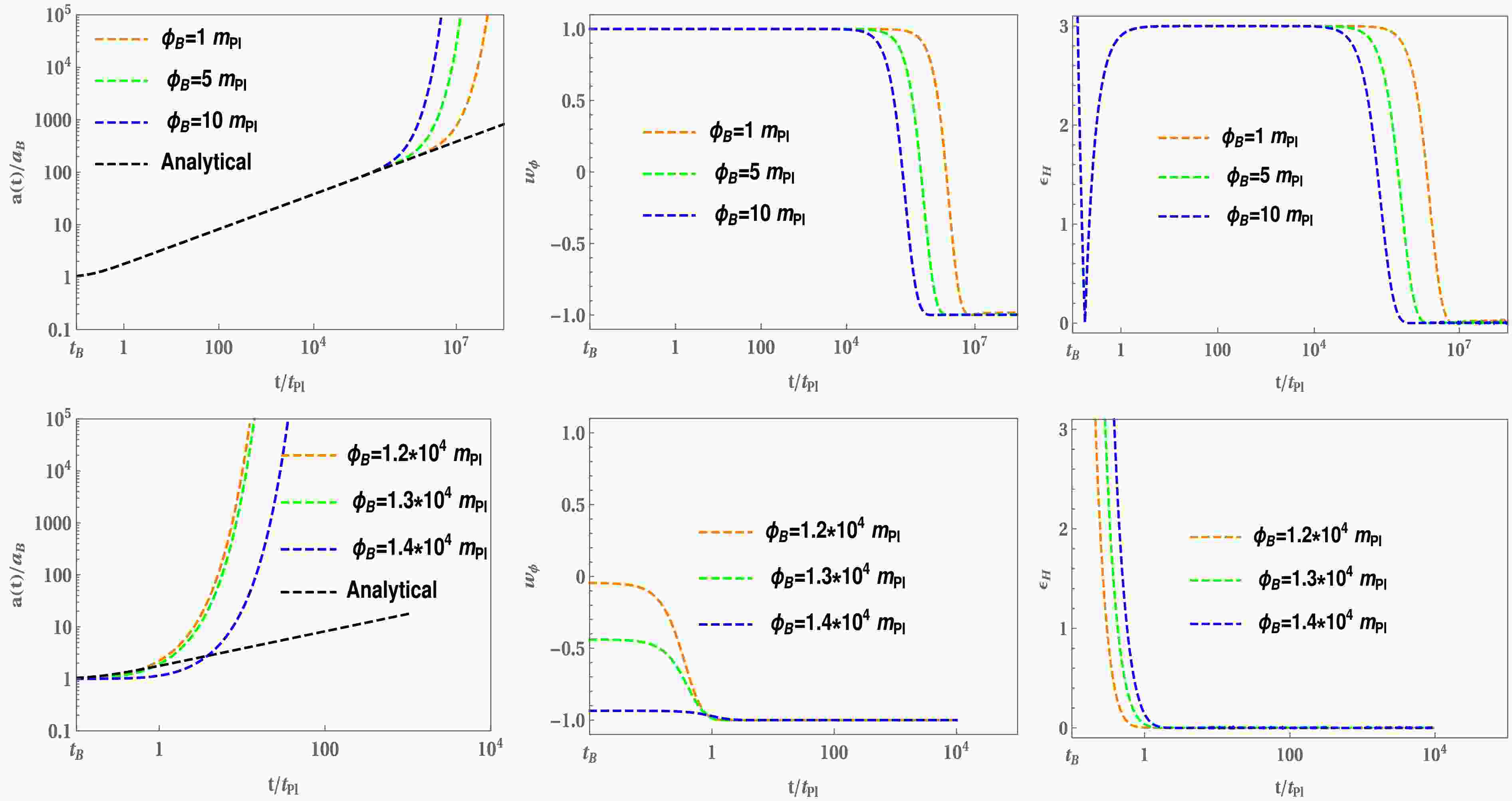
(28) We begin by analyzing the quantum bounce and subsequent slow-roll inflation for the MLFI model. The background evolution governed by Eqs. (5) and (8) is solved numerically for the potential (17), and the results are displayed in Fig. 1. For KED initial conditions of the inflaton field at the bounce (top panels), the evolution of the scale factor
$a(t)$ exhibits universal behavior during the bouncing phase. In this regime, the dynamics is independent of the initial value of the field and the specific form of the potential, and is in excellent agreement with the analytical solution (16). This universality arises because the potential energy is negligible compared to the kinetic energy throughout the bouncing phase and therefore does not affect the background evolution. The numerical evolution of the EoS$w(\phi)$ further reveals that the background dynamics can be divided into three distinct phases: the bouncing phase, the transition phase, and the slow-roll inflationary phase. The transition phase is relatively short compared to the bouncing and slow-roll phases. During the bounce, the EoS remains close to$w(\phi)\simeq+1$ , decreases from$+1$ to$-1$ during the transition phase, and then remains near$w(\phi)\simeq-1$ until the end of slow-roll inflation. Correspondingly, the Hubble slow-roll parameter satisfies$\epsilon_H>1$ in the bouncing regime, decreases rapidly from$\epsilon_H>1$ to$\epsilon_H\simeq0$ during the transition phase, and remains close to zero throughout the slow-roll inflationary era. In contrast, for PED initial conditions at the bounce (bottom panels), the universality of the scale factor$a(t)$ is no longer present. As a result, the bouncing and transition phases are not clearly distinguished. Nevertheless, a viable slow-roll inflationary phase can still be realized. The corresponding inflationary parameters, including$\epsilon_H$ ,$w(\phi)$ , and the number of e-folds,$N_{\rm{inf}}$ , are summarized in Table 1. For different initial values of$\phi_B$ , the model yields slow-roll inflation with varying durations. To be consistent with observational requirements, at least e-folds of inflation are necessary, as indicated in Table 1. It is evident from the table that the number of e-folds increases monotonically with increasing$\phi_B$ .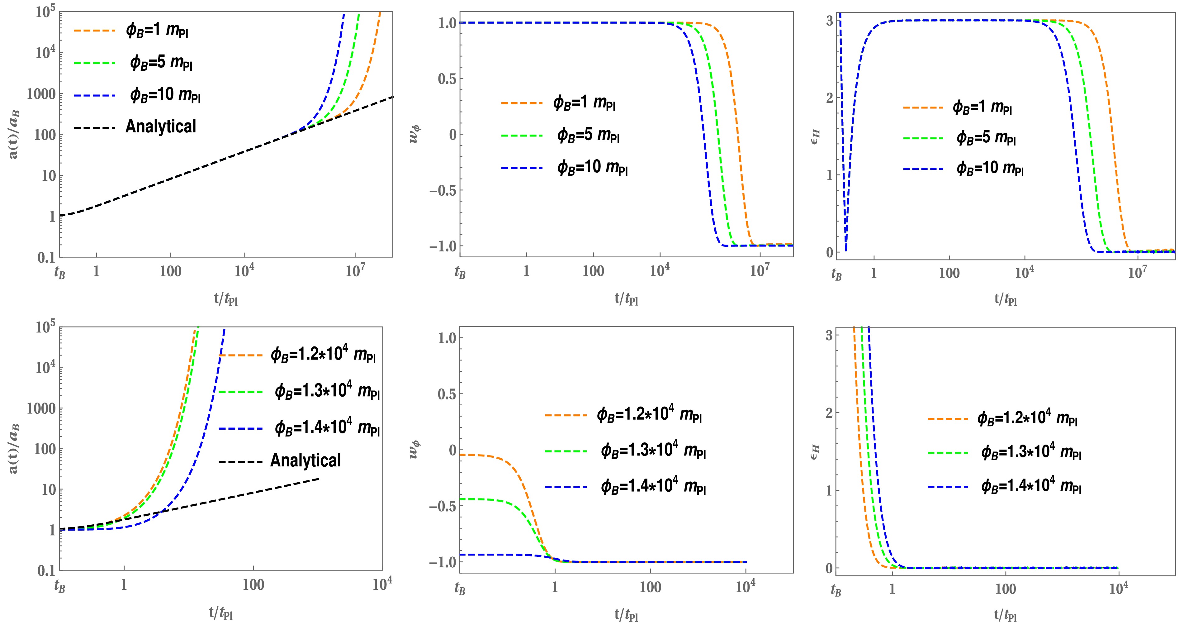
Figure 1. (color online) The figure shows the numerical evolution of
$ a(t) $ ,$ w(\phi) $ , and$ \epsilon_H $ for the mixed potential (17) with$ \dot{\phi}_B>0 $ . The upper panels correspond to KED initial conditions, and the lower panels to PED. The parameters are set to$ M=(5.705\times10^{-17}m_{Pl}^4)^{1/4} $ ,$ \alpha=1 $ , and$ m_{Pl}=1 $ . Due to the symmetry of the potential, analogous results hold for$ \dot{\phi}_B<0 $ .$\phi_B/m_{Pl}$ Inflation $t/t_{pl}$ $\epsilon_H$ $w(\phi)$ $N_{inf}$ 5 start 702173 0.999 $-1/3$ 50.0 slow-roll $2.39 \times 10^6$ $8.48 \times 10^{-5}$ $-1.0$ end $1.06 \times 10^8$ 0.268 $-1/3$ 5.5 start 621933 1.000 $-1/3$ 60.0 slow-roll $2.14 \times 10^6$ $4.88 \times 10^{-5}$ $-1.0$ end $1.28 \times 10^8$ 0.329 $-1/3$ 6 start 554535 1.000 $-1/3$ 65.4 slow-roll $1.94 \times 10^6$ $1.36 \times 10^{-4}$ $-1.0$ end $1.16 \times 10^8$ 0.325 $-1/3$ 8 start 370051 1.000 $-1/3$ 97.6 slow-roll $1.35 \times 10^6$ $1.43 \times 10^{-4}$ $-1.0$ end $1.26 \times 10^8$ 0.331 $-1/3$ Table 1. Inflationary parameters for the MLFI model with
$\dot{\phi}_B>0$ .We now compare our results with those obtained for quadratic and power-law potentials with
$n<2$ , and the Starobinsky potential, as discussed in Refs. [16, 18, 53, 54, 75, 76]. It has been shown that Starobinsky inflation is observationally viable primarily for KED initial conditions at the bounce, with only a small subset of the parameter space leading to successful inflation, while PED initial conditions are generally disfavored. In contrast, for power-law potentials with$n\leq2$ , both KED and PED initial conditions are compatible with observational requirements, particularly in terms of achieving a sufficient number of e-folds [16, 18]. In the present work, we identify physically admissible initial values of the inflaton field at the bounce and successfully realize slow-roll inflation for both KED and PED initial conditions. Our results closely resemble those obtained for the quadratic potential. A common feature of power-law inflationary models is that viable slow-roll inflation generically emerges for all allowed initial values of the inflaton field at the bounce, leading to robust and predictable inflationary outcomes. This generic behavior is absent in the Starobinsky model, where successful slow-roll inflation cannot be achieved for arbitrary initial field values. Moreover, a characteristic feature shared by most inflationary scenarios is that the pre-reheating evolution naturally separates into three distinct phases: the bouncing phase, the transition phase, and the slow-roll inflationary phase. This structure is particularly pronounced when the scalar field dynamics at the bounce is dominated by kinetic energy, with the exception of a very limited region of phase space in the Starobinsky case. As long as kinetic energy dominates at the bounce, this universal behavior remains largely independent of both the initial conditions and the specific form of the inflaton potential. We emphasize the following novel aspects of our work compared to previous studies.● We investigate a mixed quadratic-quartic potential within LQC that interpolates between two well-studied regimes.
● We demonstrate that both KED and PED initial conditions generically yield sufficient inflation.
● We identify a smooth transition from quartic to quadratic behavior that naturally facilitates slow-roll inflation without fine-tuning.
● A detailed phase-space analysis demonstrates robust attractor behavior for this class of potentials.
This distinguishes our work from previous investigations that focused on monomial or Starobinsky potentials.
-
Large-field inflation (LFI), also known as chaotic inflation [55], is characterized by simple monomial potentials of the form
$V(\phi) \propto M^4 \phi ^p$ [56−60], where the exponent p and the normalization scale M constitute the only free parameters of the model. Typically, the power p is taken to be a positive integer. However, it has been shown that such inflationary potentials may also arise naturally within supergravity [61]. Furthermore, a variety of extensions have been proposed in which p assumes rational values, motivated by string theory and effective field theory [62−67]. The MLFI model represents a natural generalization of the LFI scenario and is obtained by combining quadratic and quartic contributions. The resulting MLFI potential is given by$ V(\phi)=M^{4}\frac{\phi^{2}}{M_{Pl}^{2}}\left(1+\alpha\frac{\phi^{2}}{M_{Pl}^{2}}\right), $
(17) Here, α denotes a positive, dimensionless parameter. In the regime
$\phi/M_{Pl}\ll1/\sqrt{\alpha}$ , the potential effectively reduces to the quadratic LFI form with$p=2$ , namely$V(\phi)\simeq M^{4}\phi^{2}/M_{Pl}^{2}$ . Conversely, for$\phi/M_{Pl}\gg1/\sqrt{\alpha}$ , the quartic term dominates and the potential approaches the$p=4$ LFI limit,$V(\phi)\simeq M^{4}\alpha\phi^{4}/M_{Pl}^{4}$ . The most interesting dynamics arise in the intermediate regime$\phi/M_{Pl}\simeq1/\sqrt{\alpha}$ , where both contributions are comparable. Since$V(\phi)$ is a monotonically increasing function of the inflaton field, inflation proceeds from larger to smaller field values. The MLFI potential has been extensively explored in a variety of cosmological settings. Its form is particularly well motivated, as it corresponds to a free massive scalar field with mass-squared$M^{4}/M_{Pl}^{2}$ supplemented by a standard quartic self-interaction term. Consequently, this potential has appeared in numerous inflationary scenarios. For instance, it has been studied in the context of inflation driven by a bulk scalar field in models with large extra dimensions [68], and in scenarios where inflation arises from highly excited quantum states [69]. The same potential has also been employed in the framework of "fresh inflation" [70−72], as well as in models where the inflaton is identified with the Higgs triplet within a type-II seesaw mechanism for generating neutrino masses [73]. Moreover, it has been analyzed in supersymmetric hybrid inflation within the Randall–Sundrum type-II braneworld setup [74]. In most applications, the only phenomenological requirement is that the quartic self-interaction remains subdominant, leading to the condition$\alpha M^{4}/M_{Pl}^{4}\ll1$ . Given the typical value imposed by CMB normalization,$M/M_{Pl}\simeq10^{-3}$ , this constraint is rather mild, allowing α to span a broad range of values.The parameter M in Eq. (17) is determined from CMB normalization. The scalar amplitude inferred from CMB observations is given by
$ A_s \simeq \frac{V(\phi_*)}{24\pi^2 M_{{\rm{Pl}}}^4 \epsilon(\phi_*)}, $
(18) which can be rearranged as
$ V(\phi_*) = 24\pi^2 A_s M_{{\rm{Pl}}}^4 \epsilon(\phi_*). $
(19) The first slow-roll parameter in terms of the potential is defined as:
$ \epsilon(\phi) = \frac{M_{{\rm{Pl}}}^2}{2}\left(\frac{V'}{V}\right)^2. $
(20) Inflation ends when
$\epsilon(\phi_e) = 1$ . Therefore, we obtain the following equation.$ \frac{2}{x_{e}} \left( \frac{1 + 2\alpha x_{e}}{1 + \alpha x_{e}} \right)^{2} = 1 $
where
$x_e = \dfrac{\phi_e^2}{M_{\rm Pl}^2}$ . This equation determines$x_{e}$ and is usually solved numerically. The first slow-roll parameter and the potential at horizon crossing, i.e., at$\phi = \phi_*$ ,$ \epsilon(\phi_*) = \frac{2M_{{\rm{Pl}}}^2}{\phi_*^2} \left( \frac{1 + 2\alpha \dfrac{\phi_*^2}{M_{{\rm{Pl}}}^2}} {1 + \alpha \dfrac{\phi_*^2}{M_{{\rm{Pl}}}^2}} \right)^2. $
(21) $ V(\phi_*) = M^4 \frac{\phi_*^2}{M_{{\rm{Pl}}}^2} \left(1 + \alpha \frac{\phi_*^2}{M_{{\rm{Pl}}}^2}\right). $
(22) By substituting
$\epsilon(\phi_*)$ and$V(\phi_*)$ into the normalization condition (19), we find that the mass scale M is given by$ M = \left[ 48\pi^2 A_s \frac{M_{{\rm{Pl}}}^6}{\phi_*^4} \frac{\left(1 + 2\alpha \frac{\phi_*^2}{M_{{\rm{Pl}}}^2}\right)^2} {\left(1 + \alpha \frac{\phi_*^2}{M_{{\rm{Pl}}}^2}\right)^3} \right]^{1/4} $
(23) The number of e-folds is given by
$ \begin{aligned} N_{inf} \simeq \int_{\phi_{e}}^{\phi_*} \frac{V}{M_{{\rm{Pl}}}^2 V'{(\phi)}} {\rm d}\phi \simeq \frac{1}{8}(x_* - x_e) +\frac{1}{16\alpha} \ln\left(\frac{1+2\alpha x_*}{1+2\alpha x_e}\right), \end{aligned} $
(24) where
$ x_* \equiv \frac{\phi_*^2}{M_{{\rm{Pl}}} {^2}}. $
(25) For
$\alpha = 1$ and at large field values ($x_* \gg 1$ ), the logarithmic term is subdominant; thus, we can approximate$ N_{inf} \simeq \frac{x_*}{8}. $
(26) For
$N_{inf} = 60$ , we find$x_* \simeq 480$ . Hence,$\phi_* \simeq \sqrt{480} {M_{\rm{Pl}}}$ . Let us determine the value of M (Eq. 23) from observations of the CMB, using the measured scalar amplitude$A_s \simeq 2.09 \times 10^{-9}$ [75], with$\alpha = 1$ and$\phi_* \simeq \sqrt{480}M_{Pl}$ .$ M \approx 3 \times 10^{-4}M_{Pl}. $
(27) The quantity in Eq. (27) is expressed in units of the reduced Planck mass. We convert it to the (non-reduced) Planck mass using the relation
$M_{Pl}=m_{Pl}/ \sqrt{8 \pi}$ , and we work in units of$m_{Pl}$ throughout the paper. The model parameter M used in this paper is given by$ M \approx \left(5.705 \times 10^{-17}\right)^{1/4} m_{Pl}. $
(28) We begin by analyzing the quantum bounce and subsequent slow-roll inflation for the MLFI model. The background evolution governed by Eqs. (5) and (8) is solved numerically for the potential (17), and the results are displayed in Fig. 1. For KED initial conditions of the inflaton field at the bounce (top panels), the evolution of the scale factor
$a(t)$ exhibits universal behavior during the bouncing phase. In this regime, the dynamics is independent of the initial value of the field and the specific form of the potential, and is in excellent agreement with the analytical solution (16). This universality arises because the potential energy is negligible compared to the kinetic energy throughout the bouncing phase and therefore does not affect the background evolution. The numerical evolution of the EoS$w(\phi)$ further reveals that the background dynamics can be divided into three distinct phases: the bouncing phase, the transition phase, and the slow-roll inflationary phase. The transition phase is relatively short compared to the bouncing and slow-roll phases. During the bounce, the EoS remains close to$w(\phi)\simeq+1$ , decreases from$+1$ to$-1$ during the transition phase, and then remains near$w(\phi)\simeq-1$ until the end of slow-roll inflation. Correspondingly, the Hubble slow-roll parameter satisfies$\epsilon_H>1$ in the bouncing regime, decreases rapidly from$\epsilon_H>1$ to$\epsilon_H\simeq0$ during the transition phase, and remains close to zero throughout the slow-roll inflationary era. In contrast, for PED initial conditions at the bounce (bottom panels), the universality of the scale factor$a(t)$ is no longer present. As a result, the bouncing and transition phases are not clearly distinguished. Nevertheless, a viable slow-roll inflationary phase can still be realized. The corresponding inflationary parameters, including$\epsilon_H$ ,$w(\phi)$ , and the number of e-folds,$N_{\rm{inf}}$ , are summarized in Table 1. For different initial values of$\phi_B$ , the model yields slow-roll inflation with varying durations. To be consistent with observational requirements, at least e-folds of inflation are necessary, as indicated in Table 1. It is evident from the table that the number of e-folds increases monotonically with increasing$\phi_B$ .
Figure 1. (color online) The figure shows the numerical evolution of
$ a(t) $ ,$ w(\phi) $ , and$ \epsilon_H $ for the mixed potential (17) with$ \dot{\phi}_B>0 $ . The upper panels correspond to KED initial conditions, and the lower panels to PED. The parameters are set to$ M=(5.705\times10^{-17}m_{Pl}^4)^{1/4} $ ,$ \alpha=1 $ , and$ m_{Pl}=1 $ . Due to the symmetry of the potential, analogous results hold for$ \dot{\phi}_B<0 $ .$\phi_B/m_{Pl}$ Inflation $t/t_{pl}$ $\epsilon_H$ $w(\phi)$ $N_{inf}$ 5 start 702173 0.999 $-1/3$ 50.0 slow-roll $2.39 \times 10^6$ $8.48 \times 10^{-5}$ $-1.0$ end $1.06 \times 10^8$ 0.268 $-1/3$ 5.5 start 621933 1.000 $-1/3$ 60.0 slow-roll $2.14 \times 10^6$ $4.88 \times 10^{-5}$ $-1.0$ end $1.28 \times 10^8$ 0.329 $-1/3$ 6 start 554535 1.000 $-1/3$ 65.4 slow-roll $1.94 \times 10^6$ $1.36 \times 10^{-4}$ $-1.0$ end $1.16 \times 10^8$ 0.325 $-1/3$ 8 start 370051 1.000 $-1/3$ 97.6 slow-roll $1.35 \times 10^6$ $1.43 \times 10^{-4}$ $-1.0$ end $1.26 \times 10^8$ 0.331 $-1/3$ Table 1. Inflationary parameters for the MLFI model with
$\dot{\phi}_B>0$ .We now compare our results with those obtained for quadratic and power-law potentials with
$n<2$ , and the Starobinsky potential, as discussed in Refs. [16, 18, 53, 54, 76, 77]. It has been shown that Starobinsky inflation is observationally viable primarily for KED initial conditions at the bounce, with only a small subset of the parameter space leading to successful inflation, while PED initial conditions are generally disfavored. In contrast, for power-law potentials with$n\leq2$ , both KED and PED initial conditions are compatible with observational requirements, particularly in terms of achieving a sufficient number of e-folds [16, 18]. In the present work, we identify physically admissible initial values of the inflaton field at the bounce and successfully realize slow-roll inflation for both KED and PED initial conditions. Our results closely resemble those obtained for the quadratic potential. A common feature of power-law inflationary models is that viable slow-roll inflation generically emerges for all allowed initial values of the inflaton field at the bounce, leading to robust and predictable inflationary outcomes. This generic behavior is absent in the Starobinsky model, where successful slow-roll inflation cannot be achieved for arbitrary initial field values. Moreover, a characteristic feature shared by most inflationary scenarios is that the pre-reheating evolution naturally separates into three distinct phases: the bouncing phase, the transition phase, and the slow-roll inflationary phase. This structure is particularly pronounced when the scalar field dynamics at the bounce is dominated by kinetic energy, with the exception of a very limited region of phase space in the Starobinsky case. As long as kinetic energy dominates at the bounce, this universal behavior remains largely independent of both the initial conditions and the specific form of the inflaton potential. We emphasize the following novel aspects of our work compared to previous studies.● We investigate a mixed quadratic-quartic potential within LQC that interpolates between two well-studied regimes.
● We demonstrate that both KED and PED initial conditions generically yield sufficient inflation.
● We identify a smooth transition from quartic to quadratic behavior that naturally facilitates slow-roll inflation without fine-tuning.
● A detailed phase-space analysis demonstrates robust attractor behavior for this class of potentials.
This distinguishes our work from previous investigations that focused on monomial or Starobinsky potentials.
-
The observational viability of the inflationary model is assessed using the spectral index
$n_s$ and the tensor-to-scalar ratio r, which can be expressed in terms of the slow-roll parameters$\epsilon$ and η. The second slow-roll parameter, evaluated at horizon crossing ($\phi=\phi_*$ ), is given by$ \eta(\phi_*) = M_{Pl}^2 \frac{V"}{V} = \frac{2M_{Pl}^2}{\phi_*^2} \left( \frac{1+6\alpha\dfrac{\phi_*^2}{M_{Pl}^2}} {1+\alpha\dfrac{\phi_*^2}{M_{Pl}^2}} \right). $
(29) The inflationary observables are approximated as follows:
$ \begin{aligned} n_s &\simeq 1 - 6\epsilon(\phi_*) + 2\eta(\phi_*), \end{aligned} $
(30) $ \begin{aligned} r &\simeq 16\epsilon(\phi_*). \end{aligned} $
(31) By substituting the slow-roll parameters (21) and (29), we obtain explicit expressions for
$n_s$ and r as functions of$\phi_*$ and α. These predictions can be compared with the latest observational constraints from Planck 2018, which yield$n_s = 0.9649 \pm 0.0042$ and$r \lt 0.11$ [75].To understand the behavior of the model, we analyze three limiting cases (taking
$N_{{\rm{inf}}} = 60$ ):(A) Small-α limit (
$\alpha \phi_*^2/M_{Pl}^2 \ll 1$ ):In this regime, the model reduces to quadratic inflation. The predictions are:
$ \begin{aligned} n_s &\approx 1 - \frac{2}{N_{{\rm{inf}}}} \approx 0.967, \end{aligned} $
(32) $ \begin{aligned} r &\approx \frac{4}{N_{{\rm{inf}}}} \approx 0.067, \end{aligned} $
(33) which are consistent with observational bounds.
(B) Large α limit (
$\alpha \phi_*^2/M_{Pl}^2 \gg 1$ ):In this regime, the potential effectively behaves like quartic inflation. The corresponding predictions are:
$ \begin{aligned} n_s &\approx 1 - \frac{3}{N_{{\rm{inf}}}} \approx 0.95, \end{aligned} $
(34) $ \begin{aligned} r &\approx \frac{16}{N_{{\rm{inf}}}} \approx 0.27, \end{aligned} $
(35) These are disfavored by current observational data due to the large value of r.
(C) Intermediate α regime (
$\alpha \phi_*^2/M_{Pl}^2 \sim 1$ ):For moderate values of α, the model interpolates between the quadratic and quartic limits. For example, taking
$\alpha \sim 10^{-3}$ , which yields$\alpha \phi_*^2/M_{Pl}^2 \sim 0.4$ , one obtains$ \begin{aligned} n_s &\approx 0.962 - 0.967, \end{aligned} $
(36) $ \begin{aligned} r &\approx 0.03 - 0.05, \end{aligned} $
(37) These results lie well within the Planck-allowed region, demonstrating that the model is observationally viable in the intermediate regime. We summarize these results in Table 2.
Regime $n_s$ r Small α 0.967 0.067 Large α 0.95 0.27 Intermediate α 0.962 - 0.967 0.03 - 0.05 Planck 2018 data $0.9649 \pm 0.0042$ $< 0.11 $ Table 2. Comparison of
$n_s$ and r with observational data reported in [75]. -
The observational viability of the inflationary model is assessed using the spectral index
$n_s$ and the tensor-to-scalar ratio r, which can be expressed in terms of the slow-roll parameters$\epsilon$ and η. The second slow-roll parameter, evaluated at horizon crossing ($\phi=\phi_*$ ), is given by$ \eta(\phi_*) = M_{Pl}^2 \frac{V"}{V} = \frac{2M_{Pl}^2}{\phi_*^2} \left( \frac{1+6\alpha\dfrac{\phi_*^2}{M_{Pl}^2}} {1+\alpha\dfrac{\phi_*^2}{M_{Pl}^2}} \right). $
(29) The inflationary observables are approximated as follows:
$ \begin{aligned} n_s &\simeq 1 - 6\epsilon(\phi_*) + 2\eta(\phi_*), \end{aligned} $
(30) $ \begin{aligned} r &\simeq 16\epsilon(\phi_*). \end{aligned} $
(31) By substituting the slow-roll parameters (21) and (29), we obtain explicit expressions for
$n_s$ and r as functions of$\phi_*$ and α. These predictions can be compared with the latest observational constraints from Planck 2018, which yield$n_s = 0.9649 \pm 0.0042$ and$r \lt 0.11$ [82].To understand the behavior of the model, we analyze three limiting cases (taking
$N_{{\rm{inf}}} = 60$ ):(A) Small-α limit (
$\alpha \phi_*^2/M_{Pl}^2 \ll 1$ ):In this regime, the model reduces to quadratic inflation. The predictions are:
$ \begin{aligned} n_s &\approx 1 - \frac{2}{N_{{\rm{inf}}}} \approx 0.967, \end{aligned} $
(32) $ \begin{aligned} r &\approx \frac{4}{N_{{\rm{inf}}}} \approx 0.067, \end{aligned} $
(33) which are consistent with observational bounds.
(B) Large α limit (
$\alpha \phi_*^2/M_{Pl}^2 \gg 1$ ):In this regime, the potential effectively behaves like quartic inflation. The corresponding predictions are:
$ \begin{aligned} n_s &\approx 1 - \frac{3}{N_{{\rm{inf}}}} \approx 0.95, \end{aligned} $
(34) $ \begin{aligned} r &\approx \frac{16}{N_{{\rm{inf}}}} \approx 0.27, \end{aligned} $
(35) These are disfavored by current observational data due to the large value of r.
(C) Intermediate α regime (
$\alpha \phi_*^2/M_{Pl}^2 \sim 1$ ):For moderate values of α, the model interpolates between the quadratic and quartic limits. For example, taking
$\alpha \sim 10^{-3}$ , which yields$\alpha \phi_*^2/M_{Pl}^2 \sim 0.4$ , one obtains$ \begin{aligned} n_s &\approx 0.962 - 0.967, \end{aligned} $
(36) $ \begin{aligned} r &\approx 0.03 - 0.05, \end{aligned} $
(37) These results lie well within the Planck-allowed region, demonstrating that the model is observationally viable in the intermediate regime. We summarize these results in Table 2.
Regime $n_s$ r Small α 0.967 0.067 Large α 0.95 0.27 Intermediate α 0.962 - 0.967 0.03 - 0.05 Planck 2018 data $0.9649 \pm 0.0042$ $< 0.11 $ Table 2. Comparison of
$n_s$ and r with observational data reported in [82]. -
Phase-space analysis provides a powerful framework for investigating the qualitative behavior of dynamical systems by visualizing trajectories in an appropriate phase space. In cosmology, this approach is particularly useful for examining the evolution, stability, and asymptotic properties of cosmological models. Since the evolution of the universe can be described by a set of coupled differential equations, it naturally forms a dynamical system, often recast as an autonomous system [77-81]. Consequently, dynamical-systems techniques play a crucial role in understanding the global dynamics of such scenarios. To construct an autonomous system, it is convenient to introduce a set of dimensionless variables. This choice is motivated by several advantages: (i) it leads to a bounded phase space, (ii) the variables typically possess clear physical interpretations and remain well-behaved, and (iii) symmetries in the governing equations often allow a reduction in the number of independent equations, thereby simplifying the analysis. Accordingly, we define the following dimensionless variables:
$ Y_1=\frac{\phi}{m_{Pl}}, \quad Y_2=\frac{\dot{\phi}}{m_{Pl}^2}, \quad {\cal V}=\frac{V(Y_1)}{m_{Pl}^4}, $
(38) which allow the cosmological dynamics to be expressed as a system of first-order differential equations:
$ \begin{aligned} \frac{dY_1}{dN} =& \frac{m_{Pl} Y_2}{H(Y_1,Y_2)}, \end{aligned} $
(39) $ \begin{aligned} \frac{dY_2}{dN} =& -3Y_2 - \frac{m_{Pl}}{H(Y_1,Y_2)} \left[\frac{d{\cal V}(Y_1)}{dY_1}\right], \end{aligned} $
(40) where
$N=\ln a$ denotes the number of e-folds. The evolution equation for$Y_2$ is derived from the Klein–Gordon equation (8). The Hubble parameter that appears in Eqs. (39) and (40) is given by$ \begin{aligned} H(Y_1,Y_2)=\sqrt{\frac{8\pi m_{Pl}^2}{3} \left[\frac{Y_2^2}{2}+{\cal V}(Y_1)\right] \left[1-\frac{Y_2^2}{0.82}-\frac{{\cal V}(Y_1)}{0.41}\right]}. \end{aligned} $
(41) We numerically evolve Eqs. (39) and (40) together with Eq. (41) for the MLFI potential. The resulting phase portrait for both KED and PED initial conditions is shown in the
$(Y_1=\phi/m_{Pl},\, Y_2=\dot{\phi}/m_{Pl}^2)$ plane; see Fig. 2. The critical energy density$\rho_c$ represents the maximum allowed energy density and imposes constraints on the inflaton field at the bounce. For the potential (17), these constraints are$|\dot{\phi}_B|/m_{Pl}^2<0.91$ and$\phi_B/m_{Pl} \approx \pm 2.93$ . As a result, the black boundary in Fig. 2 is finite, reflecting the presence of the quantum gravity cutoff$\rho_c$ . At the quantum bounce ($\rho=\rho_c$ ), all trajectories originate on this boundary and subsequently evolve toward their respective minima, which correspond to stable fixed points. Regions near the boundary are associated with higher energy densities, where quantum geometric effects dominate, while trajectories approaching the minima in the$(\phi/m_{Pl},\,\dot{\phi}/m_{Pl}^2)$ plane correspond to lower energy densities and to classical behavior.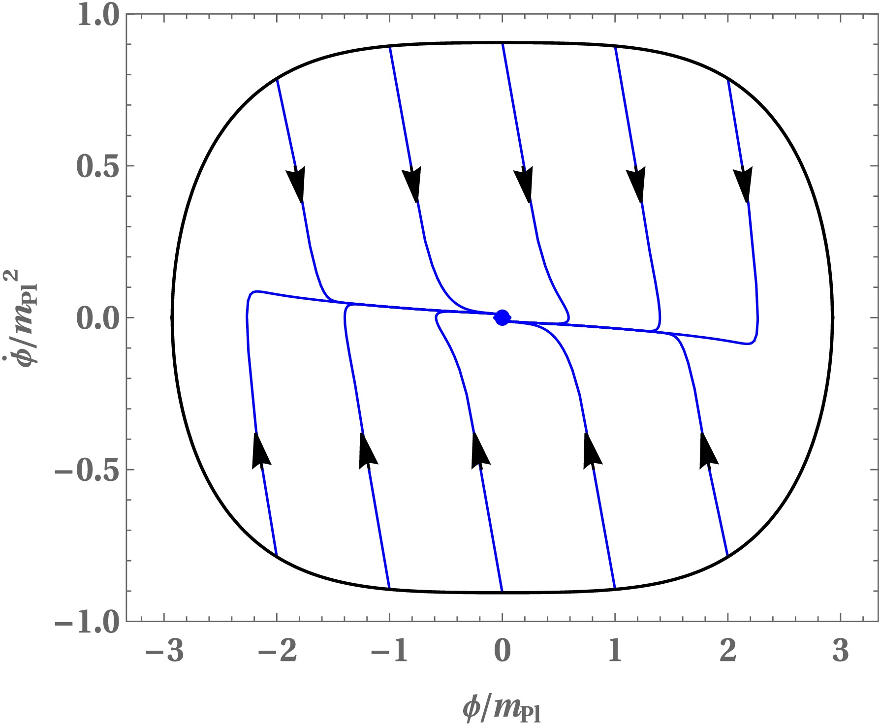
Figure 2. (color online) This figure shows the phase portrait corresponding to the potential (17) in the
$(\phi/m_{Pl},\dot{\phi}/m_{Pl}^2)$ plane. All trajectories, indicated by arrowheads, originate at the quantum bounce defined by$\rho=\rho_c$ (boundary curve) and subsequently evolve toward their minima. For visual clarity, we set$M=(0.01 m_{Pl}^4)^{1/4}$ and$\alpha=1$ . -
Phase-space analysis provides a powerful framework for investigating the qualitative behavior of dynamical systems by visualizing trajectories in an appropriate phase space. In cosmology, this approach is particularly useful for examining the evolution, stability, and asymptotic properties of cosmological models. Since the evolution of the universe can be described by a set of coupled differential equations, it naturally forms a dynamical system, often recast as an autonomous system [78−82]. Consequently, dynamical-systems techniques play a crucial role in understanding the global dynamics of such scenarios. To construct an autonomous system, it is convenient to introduce a set of dimensionless variables. This choice is motivated by several advantages: (i) it leads to a bounded phase space, (ii) the variables typically possess clear physical interpretations and remain well-behaved, and (iii) symmetries in the governing equations often allow a reduction in the number of independent equations, thereby simplifying the analysis. Accordingly, we define the following dimensionless variables:
$ Y_1=\frac{\phi}{m_{Pl}}, \quad Y_2=\frac{\dot{\phi}}{m_{Pl}^2}, \quad {\cal V}=\frac{V(Y_1)}{m_{Pl}^4}, $
(38) which allow the cosmological dynamics to be expressed as a system of first-order differential equations:
$ \begin{aligned} \frac{{\rm d}Y_1}{{\rm d}N} =& \frac{m_{Pl} Y_2}{H(Y_1,Y_2)}, \end{aligned} $
(39) $ \begin{aligned} \frac{{\rm d}Y_2}{{\rm d}N} =& -3Y_2 - \frac{m_{Pl}}{H(Y_1,Y_2)} \left[\frac{{\rm d}{\cal V}(Y_1)}{{\rm d}Y_1}\right], \end{aligned} $
(40) where
$N=\ln a$ denotes the number of e-folds. The evolution equation for$Y_2$ is derived from the Klein–Gordon equation (8). The Hubble parameter that appears in Eqs. (39) and (40) is given by$ \begin{aligned} H(Y_1,Y_2)=\sqrt{\frac{8\pi m_{Pl}^2}{3} \left[\frac{Y_2^2}{2}+{\cal V}(Y_1)\right] \left[1-\frac{Y_2^2}{0.82}-\frac{{\cal V}(Y_1)}{0.41}\right]}. \end{aligned} $
(41) We numerically evolve Eqs. (39) and (40) together with Eq. (41) for the MLFI potential. The resulting phase portrait for both KED and PED initial conditions is shown in the
$(Y_1=\phi/m_{Pl},\, Y_2=\dot{\phi}/m_{Pl}^2)$ plane; see Fig. 2. The critical energy density$\rho_c$ represents the maximum allowed energy density and imposes constraints on the inflaton field at the bounce. For the potential (17), these constraints are$|\dot{\phi}_B|/m_{Pl}^2<0.91$ and$\phi_B/m_{Pl} \approx \pm 2.93$ . As a result, the black boundary in Fig. 2 is finite, reflecting the presence of the quantum gravity cutoff$\rho_c$ . At the quantum bounce ($\rho=\rho_c$ ), all trajectories originate on this boundary and subsequently evolve toward their respective minima, which correspond to stable fixed points. Regions near the boundary are associated with higher energy densities, where quantum geometric effects dominate, while trajectories approaching the minima in the$(\phi/m_{Pl},\,\dot{\phi}/m_{Pl}^2)$ plane correspond to lower energy densities and to classical behavior.
Figure 2. (color online) This figure shows the phase portrait corresponding to the potential (17) in the
$(\phi/m_{Pl},\dot{\phi}/m_{Pl}^2)$ plane. All trajectories, indicated by arrowheads, originate at the quantum bounce defined by$\rho=\rho_c$ (boundary curve) and subsequently evolve toward their minima. For visual clarity, we set$M=(0.01 m_{Pl}^4)^{1/4}$ and$\alpha=1$ . -
The behavior of the MLFI potential within the framework of LQC exhibits a direct and physically transparent connection to the underlying bounce dynamics. In LQC, the presence of a maximum critical energy density
$\rho_c$ enforces a nonsingular quantum bounce, thereby restricting the allowed phase-space region of the inflaton field and its velocity. For the MLFI potential, which interpolates smoothly between quadratic and quartic regimes depending on the field amplitude, this bounded phase space plays a crucial role in determining the post-bounce evolution. Near the bounce, the scalar field dynamics are generically KED, rendering the specific form of the MLFI potential subdominant. As a consequence, the evolution of the scale factor in the immediate post-bounce phase exhibits the universal behavior characteristic of LQC, largely independent of the MLFI parameter α and the precise value of$\phi_B$ . As the universe expands and the energy density drops below$\rho_c$ , potential terms in the MLFI model gradually become relevant, naturally guiding the inflaton from the quartic regime at large field values toward the quadratic regime. This smooth transition facilitates the onset of slow-roll inflation without requiring fine-tuning of initial conditions. Importantly, the boundedness of the MLFI potential from below, together with the LQC-modified Friedmann dynamics, ensures that a wide range of initial conditions at the bounce, encompassing both KED and PED configurations, leads to a viable slow-roll phase with a sufficient number of e-folds. This robustness contrasts with Starobinsky inflation, where successful inflation in LQC is typically restricted to a narrower subset of KED initial conditions. The MLFI scenario thus provides a concrete realization of how LQC bounce dynamics can naturally select inflationary trajectories that are both dynamically stable and phenomenologically viable.The analysis demonstrates that the inflationary predictions of the model are highly sensitive to the parameter α, leading to distinct observational signatures in different regimes. In the small α limit, the model effectively reduces to quadratic inflation and yields values of
$n_s$ and r that are consistent with current observational bounds. In contrast, the large α regime approaches quartic inflation, which predicts a significantly larger tensor-to-scalar ratio and is therefore disfavored by the Planck 2018 data. Notably, the intermediate regime of α provides a smooth transition between these two limits and produces predictions that lie well within the observationally allowed region. For moderate values of α, the model yields a spectral index$n_s$ close to the Planck central value and a sufficiently small tensor-to-scalar ratio r. This highlights the phenomenological viability of the model and suggests that it can successfully accommodate current cosmological observations while maintaining theoretical consistency. Consequently, the intermediate α regime emerges as the most favorable region of the parameter space for describing inflation. -
In this work, we investigated the dynamical behavior of the pre-inflationary universe within the framework of LQC by considering the MLFI potential. At the quantum bounce, we numerically determined the initial values of the inflaton field that successfully led to a viable slow-roll inflationary phase with a sufficient number of e-folds. We performed a detailed numerical analysis of the cosmological evolution governed by Eqs. (5), (8) and the potential (17) with
$M=(5.705\times10^{-17}m_{Pl}^4)^{1/4}$ and$\alpha=1$ . The resulting numerical solutions, corresponding to different initial conditions of the inflaton field at the bounce, are presented in Fig. 1. The upper panels of Fig. 1 represent KED initial conditions, while the lower panels correspond to PED cases.For KED initial conditions, the numerical evolution of the scale factor
$a(t)$ exhibits a universal behavior in the bouncing regime and is in excellent agreement with the analytical solution (16). This universality arises from the negligible contribution of the potential energy compared to the kinetic energy near the bounce. As the universe evolves, the scale factor transitions to exponential growth, signaling the onset of inflation. This inflationary phase is clearly reflected in the evolution of the EoS$w(\phi)$ . Prior to preheating, the evolution of$w(\phi)$ can be divided into three distinct phases: bouncing, transition, and slow-roll inflation. During the bouncing phase,$w(\phi)\simeq +1$ , followed by a rapid decrease toward$w(\phi)\simeq-1$ in the transition phase, after which it remains close to$-1$ throughout the slow-roll regime. A similar behavior is observed for the Hubble slow-roll parameter, with$\epsilon_H>1$ at the bounce, decreasing to near zero during the transition phase and remaining small during slow-roll inflation. In contrast, for PED initial conditions at the bounce, the universality of the scale factor is lost, and the bouncing and transition phases are no longer clearly distinguishable. Nevertheless, a slow-roll inflationary phase can still be realized. To ensure compatibility with observational constraints, a minimum of e-folds of inflation is required. We demonstrate that the number of e-folds$N_{\rm{inf}}$ increases with the value of the inflaton field at the bounce, as shown in Table 1.Next, we analyzed the phase-space dynamics by constructing a phase portrait in the
$(\phi/m_{Pl},\,\dot{\phi}/m_{Pl}^2)$ plane for both positive and negative inflaton velocities, as well as for KED and PED initial conditions. For clarity of visualization, we fixed$M=(0.01\,m_{Pl}^4)^{1/4}$ . Although the potential is unbounded from above, the presence of the critical energy density$\rho_c$ in LQC constrains the allowed initial values of the inflaton field at the bounce and leads to a compact phase-space surface. The boundary curves shown in Fig. 2 correspond to the conditions$|\dot{\phi}_B|/m_{Pl}^2< 0.91$ and$\phi_B/m_{Pl} \approx \pm 2.93$ . The phase portrait revealed that all trajectories originate at the quantum bounce and are attracted toward their minima, which act as stable fixed points of the system. Finally, the inflationary predictions of the model show a strong dependence on the parameter α. The small α limit reproduces quadratic inflation and remains consistent with observational constraints, while the large α (quartic) regime is disfavored due to a large tensor-to-scalar ratio. Importantly, the intermediate regime provides a smooth interpolation between these two limits and yields predictions for$n_s$ and r that are in excellent agreement with Planck 2018 observations. Thus, the model is phenomenologically viable for moderate values of α, making it a compelling framework for describing early-universe inflation. -
In this work, we investigated the dynamical behavior of the pre-inflationary universe within the framework of LQC by considering the MLFI potential. At the quantum bounce, we numerically determined the initial values of the inflaton field that successfully led to a viable slow-roll inflationary phase with a sufficient number of e-folds. We performed a detailed numerical analysis of the cosmological evolution governed by Eqs. (5), (8) and the potential (17) with
$M=(5.705\times10^{-17}m_{Pl}^4)^{1/4}$ and$\alpha=1$ . The resulting numerical solutions, corresponding to different initial conditions of the inflaton field at the bounce, are presented in Fig. 1. The upper panels of Fig. 1 represent KED initial conditions, while the lower panels correspond to PED cases.For KED initial conditions, the numerical evolution of the scale factor
$a(t)$ exhibits a universal behavior in the bouncing regime and is in excellent agreement with the analytical solution (16). This universality arises from the negligible contribution of the potential energy compared to the kinetic energy near the bounce. As the universe evolves, the scale factor transitions to exponential growth, signaling the onset of inflation. This inflationary phase is clearly reflected in the evolution of the EoS$w(\phi)$ . Prior to preheating, the evolution of$w(\phi)$ can be divided into three distinct phases: bouncing, transition, and slow-roll inflation. During the bouncing phase,$w(\phi)\simeq+1$ , followed by a rapid decrease toward$w(\phi)\simeq-1$ in the transition phase, after which it remains close to$-1$ throughout the slow-roll regime. A similar behavior is observed for the Hubble slow-roll parameter, with$\epsilon_H>1$ at the bounce, decreasing to near zero during the transition phase and remaining small during slow-roll inflation. In contrast, for PED initial conditions at the bounce, the universality of the scale factor is lost, and the bouncing and transition phases are no longer clearly distinguishable. Nevertheless, a slow-roll inflationary phase can still be realized. To ensure compatibility with observational constraints, a minimum of e-folds of inflation is required. We demonstrate that the number of e-folds$N_{\rm{inf}}$ increases with the value of the inflaton field at the bounce, as shown in Table 1.Next, we analyzed the phase-space dynamics by constructing a phase portrait in the
$(\phi/m_{Pl},\,\dot{\phi}/m_{Pl}^2)$ plane for both positive and negative inflaton velocities, as well as for KED and PED initial conditions. For clarity of visualization, we fixed$M=(0.01\,m_{Pl}^4)^{1/4}$ . Although the potential is unbounded from above, the presence of the critical energy density$\rho_c$ in LQC constrains the allowed initial values of the inflaton field at the bounce and leads to a compact phase-space surface. The boundary curves shown in Fig. 2 correspond to the conditions$|\dot{\phi}_B|/m_{Pl}^2<0.91$ and$\phi_B/m_{Pl} \approx \pm 2.93$ . The phase portrait revealed that all trajectories originate at the quantum bounce and are attracted toward their minima, which act as stable fixed points of the system. Finally, the inflationary predictions of the model show a strong dependence on the parameter α. The small α limit reproduces quadratic inflation and remains consistent with observational constraints, while the large α (quartic) regime is disfavored due to a large tensor-to-scalar ratio. Importantly, the intermediate regime provides a smooth interpolation between these two limits and yields predictions for$n_s$ and r that are in excellent agreement with Planck 2018 observations. Thus, the model is phenomenologically viable for moderate values of α, making it a compelling framework for describing early-universe inflation.
Mixed large field inflation emerging from a quantum bounce in loop quantum cosmology
- Received Date: 2026-03-05
- Available Online: 2026-07-15
Abstract: We study the pre-inflationary evolution of the universe within the framework of loop quantum cosmology for a scalar field with potential $ V(\phi)=M^{4}\frac{\phi^{2}}{M_{Pl}^{2}}\left(1+\alpha\frac{\phi^{2}}{M_{Pl}^{2}}\right) $, where α is a positive constant. In this framework, the classical initial singularity is resolved and replaced by a non-singular quantum bounce occurring at a critical energy density. Starting from the bounce, we analyze the background dynamics for both kinetic-energy-dominated and potential-energy-dominated initial conditions. Our results show that slow-roll inflation with a sufficient number of e-folds emerges generically over a wide range of initial inflaton values. We further examine the associated phase portrait and demonstrate the attractor behavior of the slow-roll inflationary solutions. Additionally, we study the spectral index $ n_s $ and the tensor-to-scalar ratio r for three limiting cases of α, finding that the model is observationally viable in the intermediate regime.


 DownLoad: