


 Abstract
 HTML
HTML Reference
 Related
 PDF
PDF


-
Hadronic molecular states have attracted considerable theoretical interest in hadronic physics since the experimental discovery of exotic hadron states, such as
$ X(3872) $ ,$ Z_c(3900) $ ,$ Z_b(10610) $ ,$ Z_b(10650) $ , and the$ P_c $ and$ P_{cs} $ states [1−6]. Theoretically, these states are widely interpreted as hadronic molecular states. This picture has been investigated using various methods, most notably the Schrödinger equation with a one-boson-exchange (OBE) potential [7−12], the unitary approach [13−18], and the Bethe-Salpeter equation [19−26], in which the interactions are based on effective Lagrangians. In particular, because of its intuitive physical interpretation, the potential model has been progressively refined and is frequently used to describe hadronic molecular states, including the deuteron, on the basis of the Yukawa potential. The Yukawa potential was proposed to explain the strong interaction between nucleons through the exchange of a massive particle [27]. It has also been widely applied in various branches of physics, such as plasma physics, nuclear physics, astrophysics, and solid-state physics [28−37].In the context of potentials for hadronic molecular states, form factors are introduced to describe the interaction between two non-point-like particles, leading to potentials beyond the Yukawa form. These potentials are commonly used to study the binding energies of such systems. Comparisons between theoretical results and experimental data are used to determine the parameters in the form factors. The inclusion of these parameters makes the description more physical, but it also increases the complexity and obscures certain properties.
On the other hand, studies of the Schrödinger equation with the Yukawa potential reveal several interesting and elegant global properties. For a system of two nonrelativistic particles, each with mass
$ 2\mu $ , whose interaction is described by the Yukawa potential:$ V(r)=-\frac{\alpha}{r}{\rm e}^{-m_{\rm ex}r}, $
(1) where α is the coupling constant and
$ m_{\rm ex} $ represents the mass of the exchanged particle. The binding energies of this system can be described by the Schrödinger equation. When$ m_{\rm ex}=0 $ , the Yukawa potential reduces to the Coulomb potential, for which an infinite number of bound states exist, as is well established. When$ m_{\rm ex}\neq 0 $ , the situation is fundamentally different. For any finite, positive$ m_{\rm ex} $ , the number of bound states becomes finite. Moreover, there exists a critical mass beyond which no bound state can form. This phenomenon has been extensively investigated in previous studies [38−44]. These studies found that the existence of an S-wave ground-state bound state depends on the relationship among the coupling constant α, the reduced mass μ, and the exchange mass$ m_{\rm ex} $ , as given by the critical condition:$ \frac{\mu}{\alpha m_{\rm ex}} = 1.1906122105(5). $
(2) Furthermore, Refs. [39, 44, 45] systematically calculated the critical values of
$ m_{\rm ex} $ for various angular momentum states. These studies also provide the critical masses associated with the existence of the ground state, first excited state, second excited state, and higher excited states.Physically, the number of bound states is a global property of the system and is not determined by any single binding energy. For physical hadronic molecular states, once the structure of the hadrons is taken into account, a natural question is what happens to the critical behavior in these systems. In this study, we focus on the critical properties of hadronic molecular states rather than solely on their binding energies. These critical properties reflect the global nature of the system and can help us understand its internal properties. To simplify the discussion, we consider a single channel as an example.
The remainder of the article is organized as follows. In Sec. II, we present the theoretical framework, including the derivation of the Schrödinger equation and the potentials from the Bethe-Salpeter equation, and describe the numerical method employed. In Sec. III, we present our numerical results, including the critical mass
$ m_{\rm ex} $ required for the existence of bound states, the critical relationship between$ m_{\rm ex} $ and α with and without form factors, and the dependence of relevant quantities on the cutoff Λ. In addition, we give the computed binding energies as functions of α and Λ. Finally, Sec. IV summarizes our results. -
Hadronic molecular states have attracted considerable theoretical interest in hadronic physics since the experimental discovery of exotic hadron states, such as
$ X(3872) $ ,$ Z_c(3900) $ ,$ Z_b(10610) $ ,$ Z_b(10650) $ , and the$ P_c $ and$ P_{cs} $ states [1−6]. Theoretically, these states are widely interpreted as hadronic molecular states. This picture has been investigated using various methods, most notably the Schrödinger equation with a one-boson-exchange (OBE) potential [7−12], the unitary approach [13−18], and the Bethe-Salpeter equation [19−26], in which the interactions are based on effective Lagrangians. In particular, because of its intuitive physical interpretation, the potential model has been progressively refined and is frequently used to describe hadronic molecular states, including the deuteron, on the basis of the Yukawa potential. The Yukawa potential was proposed to explain the strong interaction between nucleons through the exchange of a massive particle [27]. It has also been widely applied in various branches of physics, such as plasma physics, nuclear physics, astrophysics, and solid-state physics [28−37].In the context of potentials for hadronic molecular states, form factors are introduced to describe the interaction between two non-point-like particles, leading to potentials beyond the Yukawa form. These potentials are commonly used to study the binding energies of such systems. Comparisons between theoretical results and experimental data are used to determine the parameters in the form factors. The inclusion of these parameters makes the description more physical, but it also increases the complexity and obscures certain properties.
On the other hand, studies of the Schrödinger equation with the Yukawa potential reveal several interesting and elegant global properties. For a system of two nonrelativistic particles, each with mass
$ 2\mu $ , whose interaction is described by the Yukawa potential:$ V(r)=-\frac{\alpha}{r}e^{-m_{ex}r}, $
(1) where α is the coupling constant and
$ m_{ex} $ represents the mass of the exchanged particle. The binding energies of this system can be described by the Schrödinger equation. When$ m_{ex}=0 $ , the Yukawa potential reduces to the Coulomb potential, for which an infinite number of bound states exist, as is well established. When$ m_{ex}\neq 0 $ , the situation is fundamentally different. For any finite, positive$ m_{ex} $ , the number of bound states becomes finite. Moreover, there exists a critical mass beyond which no bound state can form. This phenomenon has been extensively investigated in previous studies [38−44]. These studies found that the existence of an S-wave ground-state bound state depends on the relationship among the coupling constant α, the reduced mass μ, and the exchange mass$ m_{ex} $ , as given by the critical condition:$ \frac{\mu}{\alpha m_{ex}} = 1.1906122105(5). $
(2) Furthermore, Refs. [39, 44, 45] systematically calculated the critical values of
$ m_{ex} $ for various angular momentum states. These studies also provide the critical masses associated with the existence of the ground state, first excited state, second excited state, and higher excited states.Physically, the number of bound states is a global property of the system and is not determined by any single binding energy. For physical hadronic molecular states, once the structure of the hadrons is taken into account, a natural question is what happens to the critical behavior in these systems. In this study, we focus on the critical properties of hadronic molecular states rather than solely on their binding energies. These critical properties reflect the global nature of the system and can help us understand its internal properties. To simplify the discussion, we consider a single channel as an example.
The remainder of the article is organized as follows. In Sec. II, we present the theoretical framework, including the derivation of the Schrödinger equation and the potentials from the Bethe-Salpeter equation, and describe the numerical method employed. In Sec. III, we present our numerical results, including the critical mass
$ m_{ex} $ required for the existence of bound states, the critical relationship between$ m_{ex} $ and α with and without form factors, and the dependence of relevant quantities on the cutoff Λ. In addition, we give the computed binding energies as functions of α and Λ. Finally, Sec. IV summarizes our results. -
Hadronic molecular states have attracted considerable theoretical interest in hadronic physics since the experimental discovery of exotic hadron states, such as
$ X(3872) $ ,$ Z_c(3900) $ ,$ Z_b(10610) $ ,$ Z_b(10650) $ , and the$ P_c $ and$ P_{cs} $ states [1−6]. Theoretically, these states are widely interpreted as hadronic molecular states. This picture has been investigated using various methods, most notably the Schrödinger equation with a one-boson-exchange (OBE) potential [7−12], the unitary approach [13−18], and the Bethe-Salpeter equation [19−26], in which the interactions are based on effective Lagrangians. In particular, because of its intuitive physical interpretation, the potential model has been progressively refined and is frequently used to describe hadronic molecular states, including the deuteron, on the basis of the Yukawa potential. The Yukawa potential was proposed to explain the strong interaction between nucleons through the exchange of a massive particle [27]. It has also been widely applied in various branches of physics, such as plasma physics, nuclear physics, astrophysics, and solid-state physics [28−37].In the context of potentials for hadronic molecular states, form factors are introduced to describe the interaction between two non-point-like particles, leading to potentials beyond the Yukawa form. These potentials are commonly used to study the binding energies of such systems. Comparisons between theoretical results and experimental data are used to determine the parameters in the form factors. The inclusion of these parameters makes the description more physical, but it also increases the complexity and obscures certain properties.
On the other hand, studies of the Schrödinger equation with the Yukawa potential reveal several interesting and elegant global properties. For a system of two nonrelativistic particles, each with mass
$ 2\mu $ , whose interaction is described by the Yukawa potential:$ V(r)=-\frac{\alpha}{r}{\rm e}^{-m_{\rm ex}r}, $
(1) where α is the coupling constant and
$ m_{\rm ex} $ represents the mass of the exchanged particle. The binding energies of this system can be described by the Schrödinger equation. When$ m_{\rm ex}=0 $ , the Yukawa potential reduces to the Coulomb potential, for which an infinite number of bound states exist, as is well established. When$ m_{\rm ex}\neq 0 $ , the situation is fundamentally different. For any finite, positive$ m_{\rm ex} $ , the number of bound states becomes finite. Moreover, there exists a critical mass beyond which no bound state can form. This phenomenon has been extensively investigated in previous studies [38−44]. These studies found that the existence of an S-wave ground-state bound state depends on the relationship among the coupling constant α, the reduced mass μ, and the exchange mass$ m_{\rm ex} $ , as given by the critical condition:$ \frac{\mu}{\alpha m_{\rm ex}} = 1.1906122105(5). $
(2) Furthermore, Refs. [39, 44, 45] systematically calculated the critical values of
$ m_{\rm ex} $ for various angular momentum states. These studies also provide the critical masses associated with the existence of the ground state, first excited state, second excited state, and higher excited states.Physically, the number of bound states is a global property of the system and is not determined by any single binding energy. For physical hadronic molecular states, once the structure of the hadrons is taken into account, a natural question is what happens to the critical behavior in these systems. In this study, we focus on the critical properties of hadronic molecular states rather than solely on their binding energies. These critical properties reflect the global nature of the system and can help us understand its internal properties. To simplify the discussion, we consider a single channel as an example.
The remainder of the article is organized as follows. In Sec. II, we present the theoretical framework, including the derivation of the Schrödinger equation and the potentials from the Bethe-Salpeter equation, and describe the numerical method employed. In Sec. III, we present our numerical results, including the critical mass
$ m_{\rm ex} $ required for the existence of bound states, the critical relationship between$ m_{\rm ex} $ and α with and without form factors, and the dependence of relevant quantities on the cutoff Λ. In addition, we give the computed binding energies as functions of α and Λ. Finally, Sec. IV summarizes our results. -
For simplicity, we first consider a system of two identical scalar particles, each of mass m, whose interaction is mediated by the exchange of a third scalar particle of mass
$ m_{ex} $ . In quantum field theory (QFT), the two-body bound state of this system is described by the Bethe-Salpeter (BS) equation:$ \chi_{\text{BS}}(P,p) = \int \frac{d^4k}{(2\pi)^4}K_{\text{BS}}(p-k)G(P,k)\chi_{\text{BS}}(P,k), $
(3) where
$ \chi_{\text{BS}} $ is the BS vertex function,$ K_{\text{BS}} $ is the BS irreducible interaction kernel, and$ G(P,k) $ is the product of the propagators of the two scalar particles, expressed as$\begin{aligned}[b] G(P, k)=\;&\frac{i}{k_1^2-m^2+i \epsilon} \frac{i}{k_2^2-m^2+i \epsilon}\\=\;&\frac{-1}{(k_1^2-m^2+i \epsilon)(k_2^2-m^2+i \epsilon)}, \end{aligned}$
(4) where
$ k_1=\frac{1}{2}P+k,\; \; \; \; k_2=\frac{1}{2}P-k, $
(5) where
$ k_1 $ and$ k_2 $ are the momenta of the corresponding particles.In general, the BS equation has no analytic solution, even for
$ m_{ex} = 0 $ . When the binding energy is small compared with m, the instantaneous approximation is appropriate, meaning that:$ K_{\text{BS}}(p-k) \approx K_{\text{S}}(\boldsymbol{p}-\boldsymbol{k}). $
(6) In the center-of-mass frame, where
$ P\equiv(M,\boldsymbol{0}) $ , the instantaneous approximation and the form of$ G(P,k) $ imply that$ \chi_{\text{BS}}(P,p) $ is independent of$ p_0 $ , yielding the following equation:$ \begin{aligned}[b] \chi_{\text{S}}(M,\boldsymbol{p}) =\;& \int \frac{d^4k}{(2\pi)^4}K_{\text{S}}(\boldsymbol{p}-\boldsymbol{k})G(P,k)\chi_{\text{S}}(M,\boldsymbol{k})\\=\;&\int \frac{d^3\boldsymbol{k}}{(2\pi)^4}K_{\text{S}}(\boldsymbol{p}-\boldsymbol{k})\bar{G}(M,\boldsymbol{k})\chi_{\text{S}}(M,\boldsymbol{k}), \end{aligned} $
(7) where
$ \begin{aligned}[b] \chi_{\text{S}}(M,\boldsymbol{p}) & \equiv \chi_{\text{BS}}(P,p) \Big|_{\text{instantaneous approximation}}, \\ \bar{G}(M,\boldsymbol{k}) &\equiv \int dk_0 G(M,k)=\frac{2i\pi}{\omega_k}\frac{1}{M^2-4\omega_k^2+i\epsilon}, \end{aligned} $
(8) where
$ \omega_k=\sqrt{m^2+\boldsymbol{k}^2} $ . By defining$ \begin{array}{l} \phi_{\text{S}}(M,\boldsymbol{k})\equiv \bar{G}(M,\boldsymbol{k})\chi_{\text{S}}(M,\boldsymbol{k}), \end{array} $
(9) Eq. (7) can be equivalently written as
$ \phi_{\text{S}}(M,\boldsymbol{p}) = \bar{G}(M,\boldsymbol{p}) \int\frac{d^3\boldsymbol{k}}{(2\pi)^4} K_{\text{S}}(\boldsymbol{p}-\boldsymbol{k})\phi_{\text{S}}(M,\boldsymbol{k}), $
(10) This is the usual form of the Salpeter equation. Since
$ E_b\equiv M-2m $ and$ |\boldsymbol{p}| $ are much smaller than m, we can expand$ \bar{G}(M,\boldsymbol{k}) $ to leading order in these two small quantities, yielding the Schrödinger equation in momentum space:$ \begin{aligned}[b]& (E_b-\frac{\boldsymbol{p}^2}{m}+i\epsilon)\phi(P,\boldsymbol{p}) \\=\;& \frac{i\pi}{2m^2}\int\frac{d^3\boldsymbol{k}}{(2\pi)^4}K_{\text{S}}(\boldsymbol{p}-\boldsymbol{k}) \phi(P,\boldsymbol{k}) \\=\;& \int \frac{d^3\boldsymbol{k}}{(2\pi)^3}\Big[\frac{i K_{\text{S}}(\boldsymbol{p}-\boldsymbol{k})}{4m^2 } \Big] \phi(P,\boldsymbol{k}). \end{aligned} $
(11) The corresponding Schrödinger equation in coordinate space is therefore given by:
$ (E_b-\frac{\hat{\boldsymbol{p}}^2}{2\mu}+i\epsilon)\psi(\boldsymbol{r}) =V(\boldsymbol{r}) \psi(\boldsymbol{r}), $
(12) where
$ \mu=\dfrac{1}{2}m $ and$ \begin{aligned}[b] \psi(\boldsymbol{r}) &\equiv \int d^3{\boldsymbol{q}}e^{i\boldsymbol{q}\cdot\boldsymbol{r}} \phi(P,\boldsymbol{q}), \\ V(\boldsymbol{r}) &\equiv \int \frac{d^3{\boldsymbol{q}}}{(2\pi)^3}e^{i\boldsymbol{q}\cdot\boldsymbol{r}} i\bar{K}_{\text{S}}(\boldsymbol{q}), \end{aligned} $
(13) with
$ \bar{K}_{\text{S}}(\boldsymbol{q})\equiv \frac{1}{4m^2}K_{\text{S}}(\boldsymbol{q}). $
(14) In the present work, the Schrödinger equation is derived from the BS equation by adopting the instantaneous approximation, which effectively reduces the relativistic two-body dynamics to a nonrelativistic framework. This approximation neglects certain relativistic effects and assumes that the interaction kernel is independent of the relative time. It may become inadequate when relativistic corrections and energy-dependent effects are sizable and are not fully accounted for in the present treatment. Nevertheless, the Schrödinger equation provides a well-established and widely used framework for investigating bound-state systems. In practical applications, some relativistic effects can be effectively absorbed into model parameters, such as an effective coupling constant or the effective mass of the exchanged particle. Therefore, the present approach is expected to provide a reasonable description at the qualitative and semi-quantitative levels.
For point-like scalar particles, taking the interaction vertex for the three scalar fields as
$ \Gamma=-2igm $ gives the interaction kernel:$ \bar{K}_{\text{S}} \rightarrow \bar{K}_{0}(\boldsymbol{p}-\boldsymbol{k}) =\frac{ig^2}{(\boldsymbol{p}-\boldsymbol{k})^2+m_{ex}^2-i\epsilon}, $
(15) and the corresponding potential in coordinate space is expressed as
$ V \rightarrow V_{0}(\boldsymbol{r}) =-\frac{\alpha }{r}e^{-m_{ex}r}, $
(16) where
$ r\equiv |\boldsymbol{r}|,\alpha\equiv \dfrac{g^2}{4\pi} $ . This corresponds to a pure Yukawa potential. When the particles are not point-like, form factors are typically introduced to characterize their structure, and the corresponding correction in momentum space modifies the kernel as:$ K_{\text{S}} \rightarrow K_{1}(\boldsymbol{p}-\boldsymbol{k}) = \bar{K}_{0}(\boldsymbol{p}-\boldsymbol{k})\Big[\frac{\Lambda^2}{(\boldsymbol{p}-\boldsymbol{k})^2+\Lambda^2}\Big]^i, $
(17) where
$ i=2 $ and$ i=4 $ correspond to introducing monopole-type and dipole-type form factors at each vertex, respectively. Because the kernel contains two vertices, the choices$ i=2 $ and$ i=4 $ correspond to monopole and dipole form-factor schemes, respectively. The corresponding coordinate-space potentials with monopole and dipole form factors are given, respectively, by$ \begin{aligned}[b] V_{1}(r) =\;&-\frac{\alpha\Lambda^4}{2r(m_{ex}^2-\Lambda^2)^2}\\&\times\Big[2 e^{-m_{ex}r}-2 e^{-\Lambda r}+e^{-\Lambda r}\frac{(m_{ex}^2-\Lambda^2)r}{\Lambda}\Big],\\ V_{2}(r)=\;&-\frac{ \alpha \Lambda^8}{48 r(m_{ex}^2-\Lambda^2)^4}\\&\times\Big[48\ e^{-m_{ex} r}-48e^{-\Lambda r}+e^{-\Lambda r}P(m_{ex},\Lambda,r)\Big] \end{aligned} $
(18) where
$ \begin{aligned}[b] P(m_{ex},\Lambda,r)=\;&\frac{1}{\Lambda^5}\Big[m_{ex}^6 r[3+r\Lambda(3+r\Lambda)]\\&-3m_{ex}^4r\Lambda^2[5+r\Lambda(5+r\Lambda)]\\& +3m_{ex}^2r\Lambda^4[15+r\Lambda(7+r\Lambda)]\\&-\Lambda^5[r\Lambda(33+r\Lambda(9+r\Lambda))]\Big]. \end{aligned} $
(19) The preceding discussion can be extended to systems involving particles with other quantum numbers, for which the situation remains similar. After separating the angular part, as in the hydrogen case, the radial part of the equation in coordinate space is given, as in standard textbooks, by:
$ \Big[-\frac{1}{2\mu} \frac{\partial^2}{\partial r^2} + \frac{l(l+1)}{2\mu r^2} + V_i(r)\Big]\chi(r)=E_b\chi(r), $
(20) where l denotes the angular momentum quantum number,
$ \chi(r)\equiv r R(r) $ , and$ \psi(\boldsymbol{r})\equiv R(r)Y_{lm}(\Omega_{\boldsymbol{r}}) $ . -
For simplicity, we first consider a system of two identical scalar particles, each of mass m, whose interaction is mediated by the exchange of a third scalar particle of mass
$ m_{\rm ex} $ . In quantum field theory (QFT), the two-body bound state of this system is described by the Bethe-Salpeter (BS) equation:$ \chi_{\text{BS}}(P,p) = \int \frac{{\rm d}^4k}{(2\pi)^4}K_{\text{BS}}(p-k)G(P,k)\chi_{\text{BS}}(P,k), $
(3) where
$ \chi_{\text{BS}} $ is the BS vertex function,$ K_{\text{BS}} $ is the BS irreducible interaction kernel, and$ G(P,k) $ is the product of the propagators of the two scalar particles, expressed as$\begin{aligned}[b] G(P, k)=\;&\frac{{\rm i}}{k_1^2-m^2+ {\rm i} \epsilon} \frac{\rm i}{k_2^2-m^2+ {\rm i} \epsilon}\\=\;&\frac{-1}{(k_1^2-m^2+ {\rm i} \epsilon)(k_2^2-m^2+ {\rm i} \epsilon)}, \end{aligned}$
(4) where
$ k_1=\frac{1}{2}P+k,\; \; \; \; k_2=\frac{1}{2}P-k, $
(5) where
$ k_1 $ and$ k_2 $ are the momenta of the corresponding particles.In general, the BS equation has no analytic solution, even for
$ m_{\rm ex} = 0 $ . When the binding energy is small compared with m, the instantaneous approximation is appropriate, meaning that:$ K_{\text{BS}}(p-k) \approx K_{\text{S}}(\boldsymbol{p}-\boldsymbol{k}). $
(6) In the center-of-mass frame, where
$ P\equiv(M,\boldsymbol{0}) $ , the instantaneous approximation and the form of$ G(P,k) $ imply that$ \chi_{\text{BS}}(P,p) $ is independent of$ p_0 $ , yielding the following equation:$ \begin{aligned}[b] \chi_{\text{S}}(M,\boldsymbol{p}) =\;& \int \frac{{\rm d}^4k}{(2\pi)^4}K_{\text{S}}(\boldsymbol{p}-\boldsymbol{k})G(P,k)\chi_{\text{S}}(M,\boldsymbol{k})\\=\;&\int \frac{{\rm d}^3\boldsymbol{k}}{(2\pi)^4}K_{\text{S}}(\boldsymbol{p}-\boldsymbol{k})\bar{G}(M,\boldsymbol{k})\chi_{\text{S}}(M,\boldsymbol{k}), \end{aligned} $
(7) where
$ \begin{aligned}[b] \chi_{\text{S}}(M,\boldsymbol{p}) & \equiv \chi_{\text{BS}}(P,p) \Big|_{\text{instantaneous approximation}}, \\ \bar{G}(M,\boldsymbol{k}) &\equiv \int {\rm d} k_0 G(M,k)=\frac{2{\rm i}\pi}{\omega_k}\frac{1}{M^2-4\omega_k^2+ {\rm i}\epsilon}, \end{aligned} $
(8) where
$ \omega_k=\sqrt{m^2+\boldsymbol{k}^2} $ . By defining$ \begin{array}{l} \phi_{\text{S}}(M,\boldsymbol{k})\equiv \bar{G}(M,\boldsymbol{k})\chi_{\text{S}}(M,\boldsymbol{k}), \end{array} $
(9) Eq. (7) can be equivalently written as
$ \phi_{\text{S}}(M,\boldsymbol{p}) = \bar{G}(M,\boldsymbol{p}) \int\frac{{\rm d}^3\boldsymbol{k}}{(2\pi)^4} K_{\text{S}}(\boldsymbol{p}-\boldsymbol{k})\phi_{\text{S}}(M,\boldsymbol{k}). $
(10) This is the usual form of the Salpeter equation. Since
$ E_b\equiv M-2m $ and$ |\boldsymbol{p}| $ are much smaller than m, we can expand$ \bar{G}(M,\boldsymbol{k}) $ to leading order in these two small quantities, yielding the Schrödinger equation in momentum space:$ \begin{aligned}[b]& (E_b-\frac{\boldsymbol{p}^2}{m}+{\rm i}\epsilon)\phi(P,\boldsymbol{p}) \\=\;& \frac{{\rm i}\pi}{2m^2}\int\frac{{\rm d}^3\boldsymbol{k}}{(2\pi)^4}K_{\text{S}}(\boldsymbol{p}-\boldsymbol{k}) \phi(P,\boldsymbol{k}) \\=\;& \int \frac{{\rm d}^3\boldsymbol{k}}{(2\pi)^3}\Big[\frac{{\rm i} K_{\text{S}}(\boldsymbol{p}-\boldsymbol{k})}{4m^2 } \Big] \phi(P,\boldsymbol{k}). \end{aligned} $
(11) The corresponding Schrödinger equation in coordinate space is therefore given by:
$ \left(E_b-\frac{\hat{\boldsymbol{p}}^2}{2\mu}+{\rm i}\epsilon \right)\psi(\boldsymbol{r}) =V(\boldsymbol{r}) \psi(\boldsymbol{r}), $
(12) where
$ \mu=\dfrac{1}{2}m $ and$ \begin{aligned}[b] \psi(\boldsymbol{r}) &\equiv \int {\rm d}^3{\boldsymbol{q}}{\rm e}^{{\rm i}\boldsymbol{q}\cdot\boldsymbol{r}} \phi(P,\boldsymbol{q}), \\ V(\boldsymbol{r}) &\equiv \int \frac{{\rm d}^3{\boldsymbol{q}}}{(2\pi)^3}{\rm e}^{{\rm i}\boldsymbol{q}\cdot\boldsymbol{r}} i\bar{K}_{\text{S}}(\boldsymbol{q}), \end{aligned} $
(13) with
$ \bar{K}_{\text{S}}(\boldsymbol{q})\equiv \frac{1}{4m^2}K_{\text{S}}(\boldsymbol{q}). $
(14) In the present work, the Schrödinger equation is derived from the BS equation by adopting the instantaneous approximation, which effectively reduces the relativistic two-body dynamics to a nonrelativistic framework. This approximation neglects certain relativistic effects and assumes that the interaction kernel is independent of the relative time. It may become inadequate when relativistic corrections and energy-dependent effects are sizable and are not fully accounted for in the present treatment. Nevertheless, the Schrödinger equation provides a well-established and widely used framework for investigating bound-state systems. In practical applications, some relativistic effects can be effectively absorbed into model parameters, such as an effective coupling constant or the effective mass of the exchanged particle. Therefore, the present approach is expected to provide a reasonable description at the qualitative and semi-quantitative levels.
For point-like scalar particles, taking the interaction vertex for the three scalar fields as
$\Gamma=-2{\rm i}gm$ gives the interaction kernel:$ \bar{K}_{\text{S}} \rightarrow \bar{K}_{0}(\boldsymbol{p}-\boldsymbol{k}) =\frac{{\rm i}g^2}{(\boldsymbol{p}-\boldsymbol{k})^2+m_{\rm ex}^2-{\rm i}\epsilon}, $
(15) and the corresponding potential in coordinate space is expressed as
$ V \rightarrow V_{0}(\boldsymbol{r}) =-\frac{\alpha }{r}{\rm e}^{-m_{\rm ex}r}, $
(16) where
$ r\equiv |\boldsymbol{r}|,\alpha\equiv \dfrac{g^2}{4\pi} $ . This corresponds to a pure Yukawa potential. When the particles are not point-like, form factors are typically introduced to characterize their structure, and the corresponding correction in momentum space modifies the kernel as:$ K_{\text{S}} \rightarrow K_{1}(\boldsymbol{p}-\boldsymbol{k}) = \bar{K}_{0}(\boldsymbol{p}-\boldsymbol{k})\Big[\frac{\Lambda^2}{(\boldsymbol{p}-\boldsymbol{k})^2+\Lambda^2}\Big]^i, $
(17) where
$ i=2 $ and$ i=4 $ correspond to introducing monopole-type and dipole-type form factors at each vertex, respectively. Because the kernel contains two vertices, the choices$ i=2 $ and$ i=4 $ correspond to monopole and dipole form-factor schemes, respectively. The corresponding coordinate-space potentials with monopole and dipole form factors are given, respectively, by$ \begin{aligned}[b] V_{1}(r) =\;&-\frac{\alpha\Lambda^4}{2r(m_{\rm ex}^2-\Lambda^2)^2}\\&\times\Big[2 {\rm e}^{-m_{\rm ex}r}-2 {\rm e}^{-\Lambda r}+{\rm e}^{-\Lambda r}\frac{(m_{\rm ex}^2-\Lambda^2)r}{\Lambda}\Big],\\ V_{2}(r)=\;&-\frac{ \alpha \Lambda^8}{48 r(m_{\rm ex}^2-\Lambda^2)^4}\\&\times\Big[48\ {\rm e}^{-m_{\rm ex} r}-48e^{-\Lambda r}+{\rm e}^{-\Lambda r}P(m_{\rm ex},\Lambda,r)\Big], \end{aligned} $
(18) where
$ \begin{aligned}[b] P(m_{\rm ex},\Lambda,r)=\;&\frac{1}{\Lambda^5}\Big[m_{\rm ex}^6 r[3+r\Lambda(3+r\Lambda)]\\&-3m_{\rm ex}^4r\Lambda^2[5+r\Lambda(5+r\Lambda)]\\& +3m_{\rm ex}^2r\Lambda^4[15+r\Lambda(7+r\Lambda)]\\&-\Lambda^5[r\Lambda(33+r\Lambda(9+r\Lambda))]\Big]. \end{aligned} $
(19) The preceding discussion can be extended to systems involving particles with other quantum numbers, for which the situation remains similar. After separating the angular part, as in the hydrogen case, the radial part of the equation in coordinate space is given, as in standard textbooks, by:
$ \Big[-\frac{1}{2\mu} \frac{\partial^2}{\partial r^2} + \frac{l(l+1)}{2\mu r^2} + V_i(r)\Big]\chi(r)=E_b\chi(r), $
(20) where l denotes the angular momentum quantum number,
$ \chi(r)\equiv r R(r) $ , and$ \psi(\boldsymbol{r})\equiv R(r)Y_{lm}(\Omega_{\boldsymbol{r}}) $ . -
For simplicity, we first consider a system of two identical scalar particles, each of mass m, whose interaction is mediated by the exchange of a third scalar particle of mass
$ m_{\rm ex} $ . In quantum field theory (QFT), the two-body bound state of this system is described by the Bethe-Salpeter (BS) equation:$ \chi_{\text{BS}}(P,p) = \int \frac{{\rm d}^4k}{(2\pi)^4}K_{\text{BS}}(p-k)G(P,k)\chi_{\text{BS}}(P,k), $
(3) where
$ \chi_{\text{BS}} $ is the BS vertex function,$ K_{\text{BS}} $ is the BS irreducible interaction kernel, and$ G(P,k) $ is the product of the propagators of the two scalar particles, expressed as$\begin{aligned}[b] G(P, k)=\;&\frac{{\rm i}}{k_1^2-m^2+ {\rm i} \epsilon} \frac{\rm i}{k_2^2-m^2+ {\rm i} \epsilon}\\=\;&\frac{-1}{(k_1^2-m^2+ {\rm i} \epsilon)(k_2^2-m^2+ {\rm i} \epsilon)}, \end{aligned}$
(4) where
$ k_1=\frac{1}{2}P+k,\; \; \; \; k_2=\frac{1}{2}P-k, $
(5) where
$ k_1 $ and$ k_2 $ are the momenta of the corresponding particles.In general, the BS equation has no analytic solution, even for
$ m_{\rm ex} = 0 $ . When the binding energy is small compared with m, the instantaneous approximation is appropriate, meaning that:$ K_{\text{BS}}(p-k) \approx K_{\text{S}}(\boldsymbol{p}-\boldsymbol{k}). $
(6) In the center-of-mass frame, where
$ P\equiv(M,\boldsymbol{0}) $ , the instantaneous approximation and the form of$ G(P,k) $ imply that$ \chi_{\text{BS}}(P,p) $ is independent of$ p_0 $ , yielding the following equation:$ \begin{aligned}[b] \chi_{\text{S}}(M,\boldsymbol{p}) =\;& \int \frac{{\rm d}^4k}{(2\pi)^4}K_{\text{S}}(\boldsymbol{p}-\boldsymbol{k})G(P,k)\chi_{\text{S}}(M,\boldsymbol{k})\\=\;&\int \frac{{\rm d}^3\boldsymbol{k}}{(2\pi)^4}K_{\text{S}}(\boldsymbol{p}-\boldsymbol{k})\bar{G}(M,\boldsymbol{k})\chi_{\text{S}}(M,\boldsymbol{k}), \end{aligned} $
(7) where
$ \begin{aligned}[b] \chi_{\text{S}}(M,\boldsymbol{p}) & \equiv \chi_{\text{BS}}(P,p) \Big|_{\text{instantaneous approximation}}, \\ \bar{G}(M,\boldsymbol{k}) &\equiv \int {\rm d} k_0 G(M,k)=\frac{2{\rm i}\pi}{\omega_k}\frac{1}{M^2-4\omega_k^2+ {\rm i}\epsilon}, \end{aligned} $
(8) where
$ \omega_k=\sqrt{m^2+\boldsymbol{k}^2} $ . By defining$ \begin{array}{l} \phi_{\text{S}}(M,\boldsymbol{k})\equiv \bar{G}(M,\boldsymbol{k})\chi_{\text{S}}(M,\boldsymbol{k}), \end{array} $
(9) Eq. (7) can be equivalently written as
$ \phi_{\text{S}}(M,\boldsymbol{p}) = \bar{G}(M,\boldsymbol{p}) \int\frac{{\rm d}^3\boldsymbol{k}}{(2\pi)^4} K_{\text{S}}(\boldsymbol{p}-\boldsymbol{k})\phi_{\text{S}}(M,\boldsymbol{k}). $
(10) This is the usual form of the Salpeter equation. Since
$ E_b\equiv M-2m $ and$ |\boldsymbol{p}| $ are much smaller than m, we can expand$ \bar{G}(M,\boldsymbol{k}) $ to leading order in these two small quantities, yielding the Schrödinger equation in momentum space:$ \begin{aligned}[b]& (E_b-\frac{\boldsymbol{p}^2}{m}+{\rm i}\epsilon)\phi(P,\boldsymbol{p}) \\=\;& \frac{{\rm i}\pi}{2m^2}\int\frac{{\rm d}^3\boldsymbol{k}}{(2\pi)^4}K_{\text{S}}(\boldsymbol{p}-\boldsymbol{k}) \phi(P,\boldsymbol{k}) \\=\;& \int \frac{{\rm d}^3\boldsymbol{k}}{(2\pi)^3}\Big[\frac{{\rm i} K_{\text{S}}(\boldsymbol{p}-\boldsymbol{k})}{4m^2 } \Big] \phi(P,\boldsymbol{k}). \end{aligned} $
(11) The corresponding Schrödinger equation in coordinate space is therefore given by:
$ \left(E_b-\frac{\hat{\boldsymbol{p}}^2}{2\mu}+{\rm i}\epsilon \right)\psi(\boldsymbol{r}) =V(\boldsymbol{r}) \psi(\boldsymbol{r}), $
(12) where
$ \mu=\dfrac{1}{2}m $ and$ \begin{aligned}[b] \psi(\boldsymbol{r}) &\equiv \int {\rm d}^3{\boldsymbol{q}}{\rm e}^{{\rm i}\boldsymbol{q}\cdot\boldsymbol{r}} \phi(P,\boldsymbol{q}), \\ V(\boldsymbol{r}) &\equiv \int \frac{{\rm d}^3{\boldsymbol{q}}}{(2\pi)^3}{\rm e}^{{\rm i}\boldsymbol{q}\cdot\boldsymbol{r}} i\bar{K}_{\text{S}}(\boldsymbol{q}), \end{aligned} $
(13) with
$ \bar{K}_{\text{S}}(\boldsymbol{q})\equiv \frac{1}{4m^2}K_{\text{S}}(\boldsymbol{q}). $
(14) In the present work, the Schrödinger equation is derived from the BS equation by adopting the instantaneous approximation, which effectively reduces the relativistic two-body dynamics to a nonrelativistic framework. This approximation neglects certain relativistic effects and assumes that the interaction kernel is independent of the relative time. It may become inadequate when relativistic corrections and energy-dependent effects are sizable and are not fully accounted for in the present treatment. Nevertheless, the Schrödinger equation provides a well-established and widely used framework for investigating bound-state systems. In practical applications, some relativistic effects can be effectively absorbed into model parameters, such as an effective coupling constant or the effective mass of the exchanged particle. Therefore, the present approach is expected to provide a reasonable description at the qualitative and semi-quantitative levels.
For point-like scalar particles, taking the interaction vertex for the three scalar fields as
$\Gamma=-2{\rm i}gm$ gives the interaction kernel:$ \bar{K}_{\text{S}} \rightarrow \bar{K}_{0}(\boldsymbol{p}-\boldsymbol{k}) =\frac{{\rm i}g^2}{(\boldsymbol{p}-\boldsymbol{k})^2+m_{\rm ex}^2-{\rm i}\epsilon}, $
(15) and the corresponding potential in coordinate space is expressed as
$ V \rightarrow V_{0}(\boldsymbol{r}) =-\frac{\alpha }{r}{\rm e}^{-m_{\rm ex}r}, $
(16) where
$ r\equiv |\boldsymbol{r}|,\alpha\equiv \dfrac{g^2}{4\pi} $ . This corresponds to a pure Yukawa potential. When the particles are not point-like, form factors are typically introduced to characterize their structure, and the corresponding correction in momentum space modifies the kernel as:$ K_{\text{S}} \rightarrow K_{1}(\boldsymbol{p}-\boldsymbol{k}) = \bar{K}_{0}(\boldsymbol{p}-\boldsymbol{k})\Big[\frac{\Lambda^2}{(\boldsymbol{p}-\boldsymbol{k})^2+\Lambda^2}\Big]^i, $
(17) where
$ i=2 $ and$ i=4 $ correspond to introducing monopole-type and dipole-type form factors at each vertex, respectively. Because the kernel contains two vertices, the choices$ i=2 $ and$ i=4 $ correspond to monopole and dipole form-factor schemes, respectively. The corresponding coordinate-space potentials with monopole and dipole form factors are given, respectively, by$ \begin{aligned}[b] V_{1}(r) =\;&-\frac{\alpha\Lambda^4}{2r(m_{\rm ex}^2-\Lambda^2)^2}\\&\times\Big[2 {\rm e}^{-m_{\rm ex}r}-2 {\rm e}^{-\Lambda r}+{\rm e}^{-\Lambda r}\frac{(m_{\rm ex}^2-\Lambda^2)r}{\Lambda}\Big],\\ V_{2}(r)=\;&-\frac{ \alpha \Lambda^8}{48 r(m_{\rm ex}^2-\Lambda^2)^4}\\&\times\Big[48\ {\rm e}^{-m_{\rm ex} r}-48e^{-\Lambda r}+{\rm e}^{-\Lambda r}P(m_{\rm ex},\Lambda,r)\Big], \end{aligned} $
(18) where
$ \begin{aligned}[b] P(m_{\rm ex},\Lambda,r)=\;&\frac{1}{\Lambda^5}\Big[m_{\rm ex}^6 r[3+r\Lambda(3+r\Lambda)]\\&-3m_{\rm ex}^4r\Lambda^2[5+r\Lambda(5+r\Lambda)]\\& +3m_{\rm ex}^2r\Lambda^4[15+r\Lambda(7+r\Lambda)]\\&-\Lambda^5[r\Lambda(33+r\Lambda(9+r\Lambda))]\Big]. \end{aligned} $
(19) The preceding discussion can be extended to systems involving particles with other quantum numbers, for which the situation remains similar. After separating the angular part, as in the hydrogen case, the radial part of the equation in coordinate space is given, as in standard textbooks, by:
$ \Big[-\frac{1}{2\mu} \frac{\partial^2}{\partial r^2} + \frac{l(l+1)}{2\mu r^2} + V_i(r)\Big]\chi(r)=E_b\chi(r), $
(20) where l denotes the angular momentum quantum number,
$ \chi(r)\equiv r R(r) $ , and$ \psi(\boldsymbol{r})\equiv R(r)Y_{lm}(\Omega_{\boldsymbol{r}}) $ . -
Since the Schrödinger equation with the general potential described above cannot be solved exactly [42], we employ a numerical shooting method to solve the system with high precision. In the numerical calculation, we adopt the approximation that the wave function
$ \chi(r) $ satisfies the following boundary conditions:$ \begin{array}{l} \chi(\delta) = 0,\; \; \chi'(\delta) = 1,\; \; \chi(\Delta) = 0, \end{array} $
(21) where δ and Δ are parameters corresponding to the physical limits approaching 0 and
$ \infty $ , respectively.In the shooting method, we first fix
$ E_b $ and$ m_{\rm ex} $ and use the conditions$ \chi(\delta)=0 $ and$ \chi'(\delta) = 1 $ to solve Eq. (20) in the region$ r\in[\delta,\Delta] $ . This yields the value of$ \chi(E_b,m_{\rm ex},\Delta) $ . To determine the binding energy for a known$ m_{\rm ex} $ , we solve the equation$ \chi(E_b,m_{\rm ex},\Delta)=0 $ for the root$ E_b $ . To determine the critical value of$ m_{\rm ex} $ , we solve the equation$ \chi(0, m_{\rm ex},\Delta)=0 $ for the root$ m_{\rm ex} $ . We use a Mathematica script to implement this procedure, using the NDSolve function to solve the differential equation and FindRoot to locate the desired root. High accuracy is ensured by setting WorkingPrecision=200 and PrecisionGoal=40.In the numerical calculation of the binding energy for fixed
$ m_{\rm ex} $ and α with$ \mu=1 $ , we use the following parameter range:$ \begin{array}{l} \delta = 10^{-55} \sim 10^{-15},\; \; \Delta = 10^3\sim 10^{4}, \end{array} $
(22) where units are omitted.
In the practical calculation of the critical value of
$ m_{\rm ex} $ with$ \mu=1 $ and$ \alpha=1 $ , we set the parameters within the following range:$ \begin{array}{l} \delta = 10^{-55} \sim 10^{-15},\; \; \Delta = 10^5\sim 10^{55}. \end{array} $
(23) It is important to note that a significantly larger Δ is required to determine the critical points of the state, because the binding energy is zero. Consequently, the final results are considered acceptable only when they are stable with respect to the selected ranges of δ and Δ. For example, Table 1 lists the critical ground-state
$ m_{\rm ex} $ as a function of the integration parameters δ and Δ (cf. the exponents in columns two and three), demonstrating the stability of the results.potential $ \log_{10}\delta $ $ \log_{10}\Delta $ critical ground-state $ m_{\rm ex} $ $ V_0(r) $ –25 25 1.1906124210606177053427765163846311 –35 35 1.1906124210606177053427771063610463 –45 45 1.1906124210606177053427771063610463 –55 55 1.1906124210606177053427771063610463 $ V_1(r) $ –25 25 0.67694250611421318125252911459994898 –35 35 0.67694250611421318125252931447993144 –45 45 0.67694250611421318125252931447993146 –55 55 0.67694250611421318125252931447993146 $ V_2(r) $ –25 25 0.58558680838334368160717244234344288 –35 35 0.58558680838334368160717264884765732 –45 45 0.58558680838334368160717264884765735 –55 55 0.58558680838334368160717264884765735 Table 1. Critical ground-state value of
$ m_{\rm ex} $ as a function of$ \log_{10}\delta $ and$ \log_{10}\Delta $ for each model potential, where$ \delta=10^{k_\delta} $ and$ \Delta=10^{k_\Delta} $ , with the integers$ k_\delta,k_\Delta $ given in the table (natural units, as elsewhere in this section).Using the numerical method outlined above, we compare our results with the analytical solutions for the binding energies in the Coulomb potential case, with parameters
$ m_{\rm ex}=0 $ ,$ \alpha=1 $ , and$ \mu=1 $ . The binding energies obtained using the numerical shooting method are consistent with the analytical solutions for the Coulomb potential. Specifically, the comparison shows agreement to 35 significant digits. This high level of precision confirms the validity of our approximation and numerical method. For the case where$ m_{\rm ex}\neq 0 $ , we expect this method to achieve similar precision. -
Since the Schrödinger equation with the general potential described above cannot be solved exactly [42], we employ a numerical shooting method to solve the system with high precision. In the numerical calculation, we adopt the approximation that the wave function
$ \chi(r) $ satisfies the following boundary conditions:$ \begin{array}{l} \chi(\delta) = 0,\; \; \chi'(\delta) = 1,\; \; \chi(\Delta) = 0, \end{array} $
(21) where δ and Δ are parameters corresponding to the physical limits approaching 0 and
$ \infty $ , respectively.In the shooting method, we first fix
$ E_b $ and$ m_{\rm ex} $ and use the conditions$ \chi(\delta)=0 $ and$ \chi'(\delta) = 1 $ to solve Eq. (20) in the region$ r\in[\delta,\Delta] $ . This yields the value of$ \chi(E_b,m_{\rm ex},\Delta) $ . To determine the binding energy for a known$ m_{\rm ex} $ , we solve the equation$ \chi(E_b,m_{\rm ex},\Delta)=0 $ for the root$ E_b $ . To determine the critical value of$ m_{\rm ex} $ , we solve the equation$ \chi(0, m_{\rm ex},\Delta)=0 $ for the root$ m_{\rm ex} $ . We use a Mathematica script to implement this procedure, using the NDSolve function to solve the differential equation and FindRoot to locate the desired root. High accuracy is ensured by setting WorkingPrecision=200 and PrecisionGoal=40.In the numerical calculation of the binding energy for fixed
$ m_{\rm ex} $ and α with$ \mu=1 $ , we use the following parameter range:$ \begin{array}{l} \delta = 10^{-55} \sim 10^{-15},\; \; \Delta = 10^3\sim 10^{4}, \end{array} $
(22) where units are omitted.
In the practical calculation of the critical value of
$ m_{\rm ex} $ with$ \mu=1 $ and$ \alpha=1 $ , we set the parameters within the following range:$ \begin{array}{l} \delta = 10^{-55} \sim 10^{-15},\; \; \Delta = 10^5\sim 10^{55}. \end{array} $
(23) It is important to note that a significantly larger Δ is required to determine the critical points of the state, because the binding energy is zero. Consequently, the final results are considered acceptable only when they are stable with respect to the selected ranges of δ and Δ. For example, Table 1 lists the critical ground-state
$ m_{\rm ex} $ as a function of the integration parameters δ and Δ (cf. the exponents in columns two and three), demonstrating the stability of the results.potential $ \log_{10}\delta $ $ \log_{10}\Delta $ critical ground-state $ m_{\rm ex} $ $ V_0(r) $ –25 25 1.1906124210606177053427765163846311 –35 35 1.1906124210606177053427771063610463 –45 45 1.1906124210606177053427771063610463 –55 55 1.1906124210606177053427771063610463 $ V_1(r) $ –25 25 0.67694250611421318125252911459994898 –35 35 0.67694250611421318125252931447993144 –45 45 0.67694250611421318125252931447993146 –55 55 0.67694250611421318125252931447993146 $ V_2(r) $ –25 25 0.58558680838334368160717244234344288 –35 35 0.58558680838334368160717264884765732 –45 45 0.58558680838334368160717264884765735 –55 55 0.58558680838334368160717264884765735 Table 1. Critical ground-state value of
$ m_{\rm ex} $ as a function of$ \log_{10}\delta $ and$ \log_{10}\Delta $ for each model potential, where$ \delta=10^{k_\delta} $ and$ \Delta=10^{k_\Delta} $ , with the integers$ k_\delta,k_\Delta $ given in the table (natural units, as elsewhere in this section).Using the numerical method outlined above, we compare our results with the analytical solutions for the binding energies in the Coulomb potential case, with parameters
$ m_{\rm ex}=0 $ ,$ \alpha=1 $ , and$ \mu=1 $ . The binding energies obtained using the numerical shooting method are consistent with the analytical solutions for the Coulomb potential. Specifically, the comparison shows agreement to 35 significant digits. This high level of precision confirms the validity of our approximation and numerical method. For the case where$ m_{\rm ex}\neq 0 $ , we expect this method to achieve similar precision. -
Since the Schrödinger equation with the general potential described above cannot be solved exactly [42], we employ a numerical shooting method to solve the system with high precision. In the numerical calculation, we adopt the approximation that the wave function
$ \chi(r) $ satisfies the following boundary conditions:$ \begin{array}{l} \chi(\delta) = 0,\; \; \chi'(\delta) = 1,\; \; \chi(\Delta) = 0, \end{array} $
(21) where δ and Δ are parameters corresponding to the physical limits approaching 0 and
$ \infty $ , respectively.In the shooting method, we first fix
$ E_b $ and$ m_{ex} $ and use the conditions$ \chi(\delta)=0 $ and$ \chi'(\delta) = 1 $ to solve Eq. (20) in the region$ r\in[\delta,\Delta] $ . This yields the value of$ \chi(E_b,m_{ex},\Delta) $ . To determine the binding energy for a known$ m_{ex} $ , we solve the equation$ \chi(E_b,m_{ex},\Delta)=0 $ for the root$ E_b $ . To determine the critical value of$ m_{ex} $ , we solve the equation$ \chi(0, m_{ex},\Delta)=0 $ for the root$ m_{ex} $ . We use a Mathematica script to implement this procedure, using the NDSolve function to solve the differential equation and FindRoot to locate the desired root. High accuracy is ensured by setting WorkingPrecision=200 and PrecisionGoal=40.In the numerical calculation of the binding energy for fixed
$ m_{ex} $ and α with$ \mu=1 $ , we use the following parameter range:$ \begin{array}{l} \delta = 10^{-55} \sim 10^{-15},\; \; \Delta = 10^3\sim 10^{4}. \end{array} $
(22) where units are omitted.
In the practical calculation of the critical value of
$ m_{ex} $ with$ \mu=1 $ and$ \alpha=1 $ , we set the parameters within the following range:$ \begin{array}{l} \delta = 10^{-55} \sim 10^{-15},\; \; \Delta = 10^5\sim 10^{55}. \end{array} $
(23) It is important to note that a significantly larger Δ is required to determine the critical points of the state, because the binding energy is zero. Consequently, the final results are considered acceptable only when they are stable with respect to the selected ranges of δ and Δ. For example, Table 1 lists the critical ground-state
$ m_{ex} $ as a function of the integration parameters δ and Δ (cf. the exponents in columns two and three), demonstrating the stability of the results.potential $ \log_{10}\delta $ $ \log_{10}\Delta $ critical ground-state $ m_{ex} $ $ V_0(r) $ -25 25 1.1906124210606177053427765163846311 -35 35 1.1906124210606177053427771063610463 -45 45 1.1906124210606177053427771063610463 -55 55 1.1906124210606177053427771063610463 $ V_1(r) $ -25 25 0.67694250611421318125252911459994898 -35 35 0.67694250611421318125252931447993144 -45 45 0.67694250611421318125252931447993146 -55 55 0.67694250611421318125252931447993146 $ V_2(r) $ -25 25 0.58558680838334368160717244234344288 -35 35 0.58558680838334368160717264884765732 -45 45 0.58558680838334368160717264884765735 -55 55 0.58558680838334368160717264884765735 Table 1. Critical ground-state value of
$ m_{ex} $ as a function of$ \log_{10}\delta $ and$ \log_{10}\Delta $ for each model potential, where$ \delta=10^{k_\delta} $ and$ \Delta=10^{k_\Delta} $ , with the integers$ k_\delta,k_\Delta $ given in the table (natural units, as elsewhere in this section).Using the numerical method outlined above, we compare our results with the analytical solutions for the binding energies in the Coulomb potential case, with parameters
$ m_{ex}=0 $ ,$ \alpha=1 $ , and$ \mu=1 $ . The binding energies obtained using the numerical shooting method are consistent with the analytical solutions for the Coulomb potential. Specifically, the comparison shows agreement to 35 significant digits. This high level of precision confirms the validity of our approximation and numerical method. For the case where$ m_{ex}\neq 0 $ , we expect this method to achieve similar precision. -
For the Yukawa potential
$ V_0(r) $ , the critical value of$ m_{\rm ex} $ has been studied in Refs. [39, 42−47]. As an initial test and comparison, we present our numerical results for the critical value of$ m_{\rm ex} $ for the ground state in Table 2, with the coupling constant fixed at$ \alpha = 1 $ and the reduced mass fixed at$ \mu = 1 $ . The comparison shows that our results agree with those reported in Refs. [45−47] to approximately 30 significant digits, indicating that the shooting method is effective for obtaining high-precision results.work method value of $ m_{\rm ex} $ Ref. [39] matrix propagation 1.190612421060618 Ref. [42] fifth-order perturbative calculation 1.1906122105(5) Ref. [43, 44] hidden supersymmetry and systematic expansion 1.1906124207(2) Ref. [45] the Lagrange Mesh Method (LMM) 1.190612 Ref. [45] perturbative calculation and Padé approximations (PT) 1.19061242106061770 Ref. [46] the generalized pseudospectral (GPS) method 1.190612421060617705342777106362 Ref. [47] coupled first-order differential equations 1.19061242106061770534277710636105 this work shooting method 1.1906124210606177053427771063610463 Table 2. Comparison of the critical value of
$ m_{\rm ex} $ for the ground state, with the parameters set to$ \mu=1,\alpha=1 $ .The critical values of
$ m_{\rm ex} $ for states with other quantum numbers n and l are presented in Tables 3, 4, 5, 6. Most of our results are consistent with those reported in Refs. [39, 44, 45]. However, significant discrepancies are observed in some cases. Given that the approach employed in this work demonstrates sufficient accuracy for subsequent calculations, we conclude that the results obtained using the shooting method are reliable. These results also reveal a global property: for fixed n, the critical values of$ m_{\rm ex} $ for$ l=1 $ are always smaller than those for$ l=0 $ .Table 3. Comparison of the critical values of
$ m_{\rm ex} $ for states with principal quantum number$ n=2 $ and angular momentum quantum numbers$ l=0,1 $ in the$ V_0(r) $ case, with$ \mu=1 $ and$ \alpha=1 $ .Table 4. Comparison of the critical values of
$ m_{\rm ex} $ for states with principal quantum number$ n=3 $ and angular momentum quantum numbers$ l=0,1 $ in the$ V_0(r) $ case, with parameters$ \mu=1,\alpha=1 $ .Table 5. Comparison of the critical values of
$ m_{\rm ex} $ for states with principal quantum number$ n=4 $ and angular momentum quantum numbers$ l=0,1 $ in the$ V_0(r) $ case, with parameters$ \mu=1 $ and$ \alpha=1 $ . The notation "–" indicates that no calculation was reported in the corresponding reference.Table 6. Comparison of the critical values of
$ m_{\rm ex} $ for states with principal quantum number$ n=5 $ and angular momentum quantum numbers$ l=0 $ and$ l=1 $ in the$ V_0(r) $ case, with parameters$ \mu=1, \alpha=1 $ . The notation "–" indicates that no calculation was reported in the corresponding reference.In Tables 3–6, we present our numerical results to 35 significant digits. In practical calculations, parameters such as
$ \text{WorkingPrecision} $ and$ \text{PrecisionGoal} $ can be increased to achieve higher accuracy. Furthermore, results for other states, such as those with$ l=2 $ , can also be readily obtained but are not listed here. The complete results demonstrate that the shooting method can yield highly accurate critical values of$ m_{\rm ex} $ for states with high angular momentum (l). These high-precision values have not previously been reported in the literature.In Fig. 1, we show how the number of bound states depends on the parameters
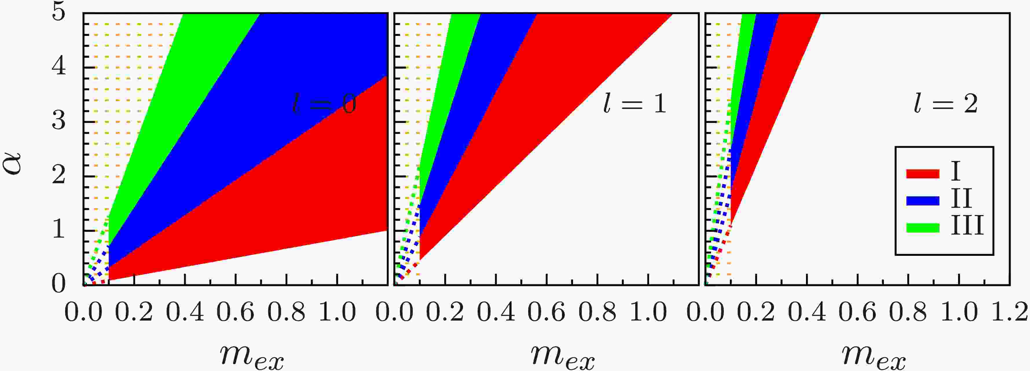
$ m_{\rm ex} $ and α. The panels, ordered from left to right, correspond to$ l=0 $ ,$ l=1 $ , and$ l=2 $ . The red (I), blue (II), and green (III) regions indicate the presence of one, two, and three bound states, respectively, for the given l. The dotted region denotes an area outside the scope of our discussion. Our calculations specifically consider the region where$ m_{\rm ex}\geq0.1 $ . The dashed lines show the critical-boundary curves obtained from our discrete numerical points and extrapolated toward smaller$ m_{\rm ex} $ in the$ (\alpha,m_{\rm ex}) $ plane, as justified below. We extrapolate the critical boundaries toward the origin for two reasons. First, when$ m_{\rm ex}\rightarrow 0 $ , bound states exist for any sufficiently small positive α, whereas none exist for$ \alpha=0 $ . Therefore, both α and$ m_{\rm ex} $ must approach zero along the critical line. Second, within the computed parameter range, we observe an approximately linear relation between the critical coupling α and$ m_{\rm ex} $ . Following this trend, the boundary curves are extended to smaller$ m_{\rm ex} $ and visually appear to converge to the origin as$ \alpha\rightarrow 0 $ . For the specific case of$ l=0 $ and$ \alpha=1 $ , the critical value of$ m_{\rm ex} $ is approximately$ 1.19 $ , consistent with the data presented in Table 2. We observe that the slope of the boundary curve increases with the orbital angular momentum quantum number l. This indicates that a larger coupling constant is required to form a bound state as l increases. Furthermore, the linear behavior of the region boundaries directly indicates that the critical values satisfy relations similar to Eq. (2). Such relations can, in fact, be determined through dimensional analysis.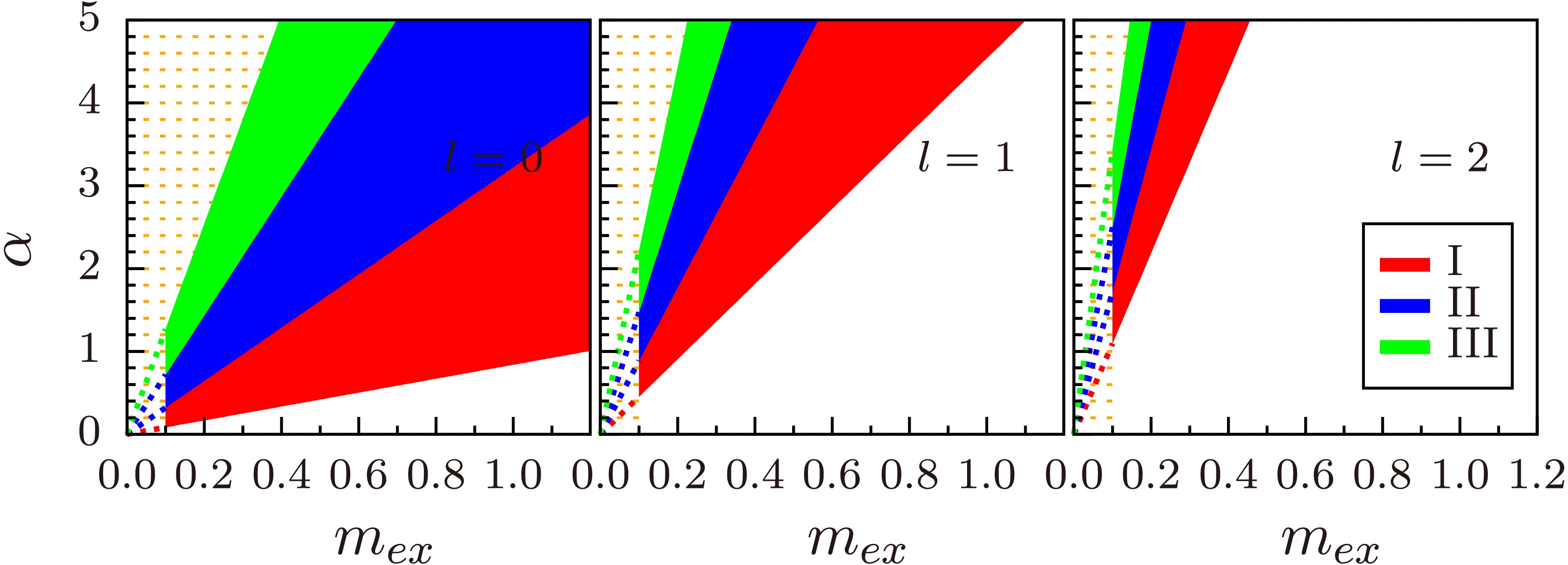
Figure 1. (color online) Critical boundaries for the number of bound states as functions of α and
$ m_{\rm ex} $ for specified angular momentum l in the$ V_0(r) $ case, with μ fixed at$ 1 $ . The panels, ordered from left to right, show the cases$ l=0 $ ,$ l=1 $ , and$ l=2 $ . The red (I), blue (II), and green (III) regions indicate the existence of one, two, and three bound states, respectively. -
For the Yukawa potential
$ V_0(r) $ , the critical value of$ m_{ex} $ has been studied in Refs. [39, 42−47]. As an initial test and comparison, we present our numerical results for the critical value of$ m_{ex} $ for the ground state in Table 2, with the coupling constant fixed at$ \alpha = 1 $ and the reduced mass fixed at$ \mu = 1 $ . The comparison shows that our results agree with those reported in Refs. [45−47] to approximately 30 significant digits, indicating that the shooting method is effective for obtaining high-precision results.work method value of $ m_{ex} $ Ref. [39] matrix propagation 1.190612421060618 Ref. [42] fifth-order perturbative calculation 1.1906122105(5) Ref. [43, 44] hidden supersymmetry and systematic expansion 1.1906124207(2) Ref. [45] the Lagrange Mesh Method (LMM) 1.190612 Ref. [45] perturbative calculation and Padé approximations (PT) 1.19061242106061770 Ref. [46] the generalized pseudospectral (GPS) method 1.190612421060617705342777106362 Ref. [47] coupled first-order differential equations 1.19061242106061770534277710636105 this work shooting method 1.1906124210606177053427771063610463 Table 2. Comparison of the critical value of
$ m_{ex} $ for the ground state, with the parameters set to$ \mu=1,\alpha=1 $ .The critical values of
$ m_{ex} $ for states with other quantum numbers n and l are presented in Tables 3,4,5,6. Most of our results are consistent with those reported in Refs. [39, 44, 45]. However, significant discrepancies are observed in some cases. Given that the approach employed in this work demonstrates sufficient accuracy for subsequent calculations, we conclude that the results obtained using the shooting method are reliable. These results also reveal a global property: for fixed n, the critical values of$ m_{ex} $ for$ l=1 $ are always smaller than those for$ l=0 $ .Table 3. Comparison of the critical values of
$ m_{ex} $ for states with principal quantum number$ n=2 $ and angular momentum quantum numbers$ l=0,1 $ in the$ V_0(r) $ case, with$ \mu=1 $ and$ \alpha=1 $ .Table 4. Comparison of the critical values of
$ m_{ex} $ for states with principal quantum number$ n=3 $ and angular momentum quantum numbers$ l=0,1 $ in the$ V_0(r) $ case, with parameters$ \mu=1,\alpha=1 $ .Table 5. Comparison of the critical values of
$ m_{ex} $ for states with principal quantum number$ n=4 $ and angular momentum quantum numbers$ l=0,1 $ in the$ V_0(r) $ case, with parameters$ \mu=1 $ and$ \alpha=1 $ . The notation "–" indicates that no calculation was reported in the corresponding reference.Table 6. Comparison of the critical values of
$ m_{ex} $ for states with principal quantum number$ n=5 $ and angular momentum quantum numbers$ l=0 $ and$ l=1 $ in the$ V_0(r) $ case, with parameters$ \mu=1, \alpha=1 $ . The notation "–" indicates that no calculation was reported in the corresponding reference.In Tables 3–6, we present our numerical results to 35 significant digits. In practical calculations, parameters such as
$ \text{WorkingPrecision} $ and$ \text{PrecisionGoal} $ can be increased to achieve higher accuracy. Furthermore, results for other states, such as those with$ l=2 $ , can also be readily obtained but are not listed here. The complete results demonstrate that the shooting method can yield highly accurate critical values of$ m_{ex} $ for states with high angular momentum (l). These high-precision values have not previously been reported in the literature.In Fig. 1, we show how the number of bound states depends on the parameters
$ m_{ex} $ and α. The panels, ordered from left to right, correspond to$ l=0 $ ,$ l=1 $ , and$ l=2 $ . The red (I), blue (II), and green (III) regions indicate the presence of one, two, and three bound states, respectively, for the given l. The dotted region denotes an area outside the scope of our discussion. Our calculations specifically consider the region where$ m_{ex}\geq0.1 $ . The dashed lines show the critical-boundary curves obtained from our discrete numerical points and extrapolated toward smaller$ m_{ex} $ in the$ (\alpha,m_{ex}) $ plane, as justified below. We extrapolate the critical boundaries toward the origin for two reasons. First, when$ m_{ex}\rightarrow 0 $ , bound states exist for any sufficiently small positive α, whereas none exist for$ \alpha=0 $ . Therefore, both α and$ m_{ex} $ must approach zero along the critical line. Second, within the computed parameter range, we observe an approximately linear relation between the critical coupling α and$ m_{ex} $ . Following this trend, the boundary curves are extended to smaller$ m_{ex} $ and visually appear to converge to the origin as$ \alpha\rightarrow 0 $ . For the specific case of$ l=0 $ and$ \alpha=1 $ , the critical value of$ m_{ex} $ is approximately$ 1.19 $ , consistent with the data presented in Table 2. We observe that the slope of the boundary curve increases with the orbital angular momentum quantum number l. This indicates that a larger coupling constant is required to form a bound state as l increases. Furthermore, the linear behavior of the region boundaries directly indicates that the critical values satisfy relations similar to Eq. (2). Such relations can, in fact, be determined through dimensional analysis.
Figure 1. (color online) Critical boundaries for the number of bound states as functions of α and
$ m_{ex} $ for specified angular momentum l in the$ V_0(r) $ case, with μ fixed at$ 1 $ . The panels, ordered from left to right, show the cases$ l=0 $ ,$ l=1 $ , and$ l=2 $ . The red (I), blue (II), and green (III) regions indicate the existence of one, two, and three bound states, respectively. -
For the Yukawa potential
$ V_0(r) $ , the critical value of$ m_{\rm ex} $ has been studied in Refs. [39, 42−47]. As an initial test and comparison, we present our numerical results for the critical value of$ m_{\rm ex} $ for the ground state in Table 2, with the coupling constant fixed at$ \alpha = 1 $ and the reduced mass fixed at$ \mu = 1 $ . The comparison shows that our results agree with those reported in Refs. [45−47] to approximately 30 significant digits, indicating that the shooting method is effective for obtaining high-precision results.work method value of $ m_{\rm ex} $ Ref. [39] matrix propagation 1.190612421060618 Ref. [42] fifth-order perturbative calculation 1.1906122105(5) Ref. [43, 44] hidden supersymmetry and systematic expansion 1.1906124207(2) Ref. [45] the Lagrange Mesh Method (LMM) 1.190612 Ref. [45] perturbative calculation and Padé approximations (PT) 1.19061242106061770 Ref. [46] the generalized pseudospectral (GPS) method 1.190612421060617705342777106362 Ref. [47] coupled first-order differential equations 1.19061242106061770534277710636105 this work shooting method 1.1906124210606177053427771063610463 Table 2. Comparison of the critical value of
$ m_{\rm ex} $ for the ground state, with the parameters set to$ \mu=1,\alpha=1 $ .The critical values of
$ m_{\rm ex} $ for states with other quantum numbers n and l are presented in Tables 3, 4, 5, 6. Most of our results are consistent with those reported in Refs. [39, 44, 45]. However, significant discrepancies are observed in some cases. Given that the approach employed in this work demonstrates sufficient accuracy for subsequent calculations, we conclude that the results obtained using the shooting method are reliable. These results also reveal a global property: for fixed n, the critical values of$ m_{\rm ex} $ for$ l=1 $ are always smaller than those for$ l=0 $ .Table 3. Comparison of the critical values of
$ m_{\rm ex} $ for states with principal quantum number$ n=2 $ and angular momentum quantum numbers$ l=0,1 $ in the$ V_0(r) $ case, with$ \mu=1 $ and$ \alpha=1 $ .Table 4. Comparison of the critical values of
$ m_{\rm ex} $ for states with principal quantum number$ n=3 $ and angular momentum quantum numbers$ l=0,1 $ in the$ V_0(r) $ case, with parameters$ \mu=1,\alpha=1 $ .Table 5. Comparison of the critical values of
$ m_{\rm ex} $ for states with principal quantum number$ n=4 $ and angular momentum quantum numbers$ l=0,1 $ in the$ V_0(r) $ case, with parameters$ \mu=1 $ and$ \alpha=1 $ . The notation "–" indicates that no calculation was reported in the corresponding reference.Table 6. Comparison of the critical values of
$ m_{\rm ex} $ for states with principal quantum number$ n=5 $ and angular momentum quantum numbers$ l=0 $ and$ l=1 $ in the$ V_0(r) $ case, with parameters$ \mu=1, \alpha=1 $ . The notation "–" indicates that no calculation was reported in the corresponding reference.In Tables 3–6, we present our numerical results to 35 significant digits. In practical calculations, parameters such as
$ \text{WorkingPrecision} $ and$ \text{PrecisionGoal} $ can be increased to achieve higher accuracy. Furthermore, results for other states, such as those with$ l=2 $ , can also be readily obtained but are not listed here. The complete results demonstrate that the shooting method can yield highly accurate critical values of$ m_{\rm ex} $ for states with high angular momentum (l). These high-precision values have not previously been reported in the literature.In Fig. 1, we show how the number of bound states depends on the parameters
$ m_{\rm ex} $ and α. The panels, ordered from left to right, correspond to$ l=0 $ ,$ l=1 $ , and$ l=2 $ . The red (I), blue (II), and green (III) regions indicate the presence of one, two, and three bound states, respectively, for the given l. The dotted region denotes an area outside the scope of our discussion. Our calculations specifically consider the region where$ m_{\rm ex}\geq0.1 $ . The dashed lines show the critical-boundary curves obtained from our discrete numerical points and extrapolated toward smaller$ m_{\rm ex} $ in the$ (\alpha,m_{\rm ex}) $ plane, as justified below. We extrapolate the critical boundaries toward the origin for two reasons. First, when$ m_{\rm ex}\rightarrow 0 $ , bound states exist for any sufficiently small positive α, whereas none exist for$ \alpha=0 $ . Therefore, both α and$ m_{\rm ex} $ must approach zero along the critical line. Second, within the computed parameter range, we observe an approximately linear relation between the critical coupling α and$ m_{\rm ex} $ . Following this trend, the boundary curves are extended to smaller$ m_{\rm ex} $ and visually appear to converge to the origin as$ \alpha\rightarrow 0 $ . For the specific case of$ l=0 $ and$ \alpha=1 $ , the critical value of$ m_{\rm ex} $ is approximately$ 1.19 $ , consistent with the data presented in Table 2. We observe that the slope of the boundary curve increases with the orbital angular momentum quantum number l. This indicates that a larger coupling constant is required to form a bound state as l increases. Furthermore, the linear behavior of the region boundaries directly indicates that the critical values satisfy relations similar to Eq. (2). Such relations can, in fact, be determined through dimensional analysis.
Figure 1. (color online) Critical boundaries for the number of bound states as functions of α and
$ m_{\rm ex} $ for specified angular momentum l in the$ V_0(r) $ case, with μ fixed at$ 1 $ . The panels, ordered from left to right, show the cases$ l=0 $ ,$ l=1 $ , and$ l=2 $ . The red (I), blue (II), and green (III) regions indicate the existence of one, two, and three bound states, respectively. -
The potential
$ V_1(r) $ is widely used to study molecular states within OBE models. Its critical parameters reflect the global properties of the system and are crucial for understanding the internal properties of the bound states. In this subsection, we discuss the properties associated with this potential. For simplicity, we continue to use the scalar system as an example.Table 7 provides the critical values of
$ m_{ex} $ for$ \mu=1 $ ,$ \alpha=1 $ , and$ \Lambda=1 $ , classified according to the quantum numbers n and l. Because no comparable results for the critical mass in the$ V_1 $ case are available in the literature, Table 7 reports only our values. Fig. 2 illustrates how the number of bound states evolves with the parameters$ m_{ex} $ and α, with Λ and μ fixed, using the same notation as in Fig. 1. Similarly, Fig. 3 shows how the number of bound states evolves with the parameters α and Λ, with$ m_{ex} $ and μ fixed.n l 0 1 1 0.67694250611421318125252931447993146 – 2 0.20562081503354359818299315422443232 0.20695075065871335259276932355973134 3 0.10387929422723629079373251602398867 0.10384898223045325459958290388192965 4 0.062812729606088808273694095206222191 0.063137840555479296025152192163701117 5 0.042070819608385184596535181069213768 0.042454393767796674198021311139945282 Table 7. The critical values of
$ m_{ex} $ for$ \mu=1 $ ,$ \alpha=1 $ , and$ \Lambda=1 $ , categorized by the quantum numbers n and l for the$ V_1(r) $ case.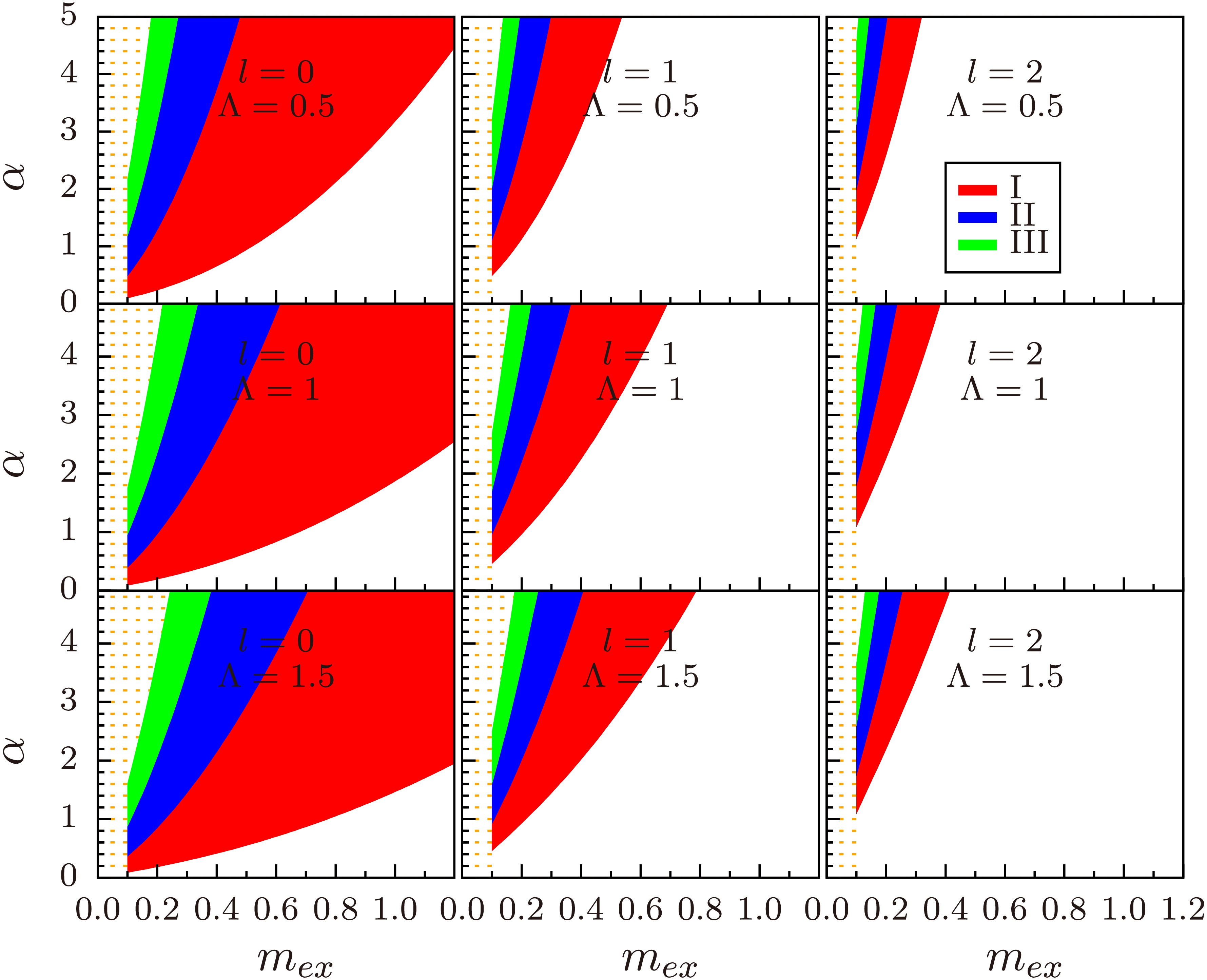
Figure 2. (color online) Critical boundaries of regions with different numbers of bound states as functions of α and
$ m_{ex} $ for fixed angular momentum l and cutoff Λ for the$ V_1(r) $ potential, with μ fixed at$ 1 $ . The panels, ordered from left to right, show the cases$ l=0 $ ,$ l=1 $ , and$ l=2 $ . The red (I), blue (II), and green (III) regions indicate the existence of one, two, and three bound states, respectively.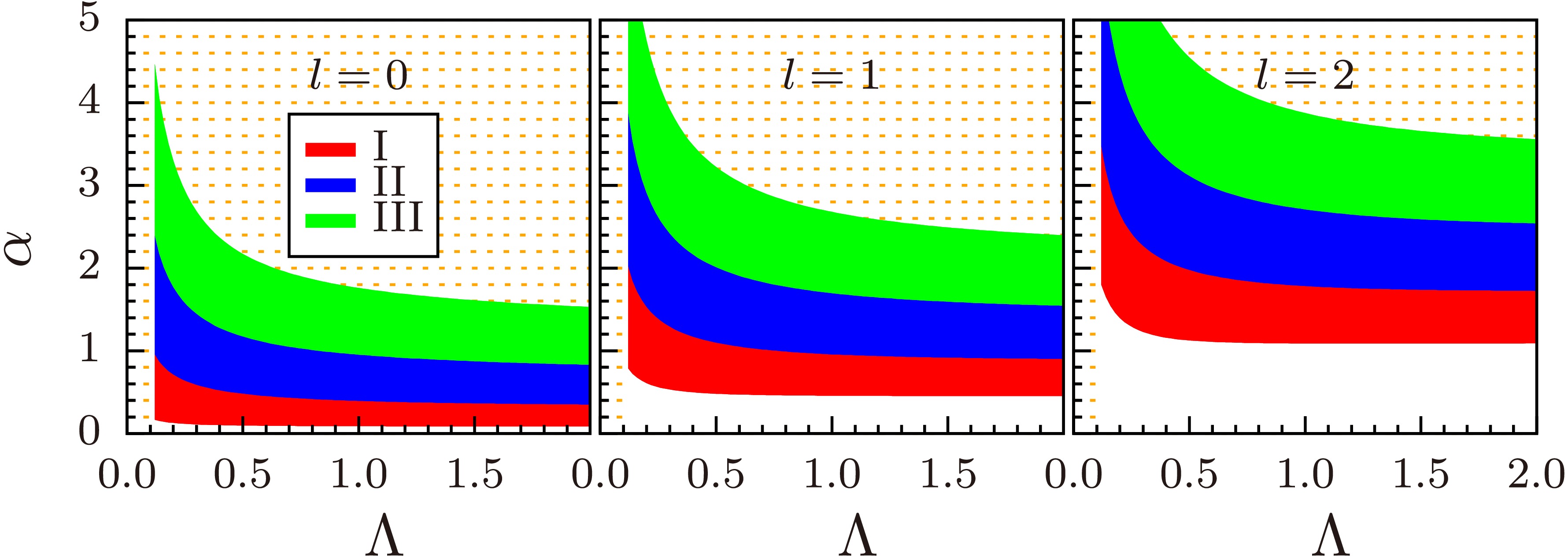
Figure 3. (color online) Critical boundaries for the number of bound states as functions of α and Λ for specified angular momenta l in the
$ V_1(r) $ case, with μ fixed at$ 1 $ and$ m_{ex} $ fixed at$ 0.1 $ . The panels, from left to right, show the cases$ l=0 $ ,$ l=1 $ , and$ l=2 $ . The red (I), blue (II), and green (III) regions indicate the existence of one, two, and three bound states, respectively.The results in Table 7 show an interesting feature that differs markedly from the
$ V_0 $ case: for some quantum numbers n, the critical value of$ m_{ex} $ in the$ l=1 $ case is larger than that in the$ l=0 $ case. The results in Fig. 2 also exhibit behavior distinct from that in the$ V_0 $ case: the boundaries of the regions are no longer straight. This indicates that, for finite Λ, the critical values of$ m_{ex} $ and α do not satisfy a linear relation analogous to Eq. (2). In addition, when$ m_{ex} $ is fixed, the corresponding critical value of α decreases as the cutoff Λ increases. This suggests that a smaller cutoff Λ has a more pronounced effect on the existence of bound states.The results in Fig. 3, with
$ m_{ex}=0.1 $ and$ \mu=1 $ , show that the critical values of α for the ground state depend only weakly on Λ. This suggests that varying Λ does not substantially alter the number of bound states in the large-Λ regime, particularly for the ground state. To illustrate this explicitly, we provide a short numerical table, Table 8, from which the trend can be read directly.Λ $ \alpha(l=0,n=1) $ $ \alpha(l=0,n=2) $ $ \alpha(l=0,n=3) $ $ \alpha(l=0,n=4) $ 0.5 0.096 0.482 1.173 2.171 1.0 0.088 0.395 0.954 1.760 1.5 0.086 0.365 0.874 1.610 2.0 0.085 0.351 0.832 1.530 2.5 0.085 0.343 0.806 1.479 3.0 0.085 0.338 0.788 1.443 3.5 0.084 0.335 0.775 1.417 4.0 0.084 0.332 0.766 1.397 Table 8. The critical values of α as functions of Λ in the case of
$ V_1(r) $ for$ l=0 $ , with μ fixed at$ 1 $ and$ m_{ex} $ fixed at$ 0.1 $ . -
The potential
$ V_1(r) $ is widely used to study molecular states within OBE models. Its critical parameters reflect the global properties of the system and are crucial for understanding the internal properties of the bound states. In this subsection, we discuss the properties associated with this potential. For simplicity, we continue to use the scalar system as an example.Table 7 provides the critical values of
$ m_{\rm ex} $ for$ \mu=1 $ ,$ \alpha=1 $ , and$ \Lambda=1 $ , classified according to the quantum numbers n and l. Because no comparable results for the critical mass in the$ V_1 $ case are available in the literature, Table 7 reports only our values. Figure 2 illustrates how the number of bound states evolves with the parameters$ m_{\rm ex} $ and α, with Λ and μ fixed, using the same notation as in Fig. 1. Similarly, Fig. 3 shows how the number of bound states evolves with the parameters α and Λ, with$ m_{\rm ex} $ and μ fixed.n l 0 1 1 0.67694250611421318125252931447993146 – 2 0.20562081503354359818299315422443232 0.20695075065871335259276932355973134 3 0.10387929422723629079373251602398867 0.10384898223045325459958290388192965 4 0.062812729606088808273694095206222191 0.063137840555479296025152192163701117 5 0.042070819608385184596535181069213768 0.042454393767796674198021311139945282 Table 7. The critical values of
$ m_{\rm ex} $ for$ \mu=1 $ ,$ \alpha=1 $ , and$ \Lambda=1 $ , categorized by the quantum numbers n and l for the$ V_1(r) $ case.
Figure 2. (color online) Critical boundaries of regions with different numbers of bound states as functions of α and
$ m_{\rm ex} $ for fixed angular momentum l and cutoff Λ for the$ V_1(r) $ potential, with μ fixed at$ 1 $ . The panels, ordered from left to right, show the cases$ l=0 $ ,$ l=1 $ , and$ l=2 $ . The red (I), blue (II), and green (III) regions indicate the existence of one, two, and three bound states, respectively.
Figure 3. (color online) Critical boundaries for the number of bound states as functions of α and Λ for specified angular momenta l in the
$ V_1(r) $ case, with μ fixed at$ 1 $ and$ m_{\rm ex} $ fixed at$ 0.1 $ . The panels, from left to right, show the cases$ l=0 $ ,$ l=1 $ , and$ l=2 $ . The red (I), blue (II), and green (III) regions indicate the existence of one, two, and three bound states, respectively.The results in Table 7 show an interesting feature that differs markedly from the
$ V_0 $ case: for some quantum numbers n, the critical value of$ m_{\rm ex} $ in the$ l=1 $ case is larger than that in the$ l=0 $ case. The results in Fig. 2 also exhibit behavior distinct from that in the$ V_0 $ case: the boundaries of the regions are no longer straight. This indicates that, for finite Λ, the critical values of$ m_{\rm ex} $ and α do not satisfy a linear relation analogous to Eq. (2). In addition, when$ m_{\rm ex} $ is fixed, the corresponding critical value of α decreases as the cutoff Λ increases. This suggests that a smaller cutoff Λ has a more pronounced effect on the existence of bound states.The results in Fig. 3, with
$ m_{\rm ex}=0.1 $ and$ \mu=1 $ , show that the critical values of α for the ground state depend only weakly on Λ. This suggests that varying Λ does not substantially alter the number of bound states in the large-Λ regime, particularly for the ground state. To illustrate this explicitly, we provide a short numerical table, Table 8, from which the trend can be read directly.Λ $ \alpha(l=0,n=1) $ $ \alpha(l=0,n=2) $ $ \alpha(l=0,n=3) $ $ \alpha(l=0,n=4) $ 0.5 0.096 0.482 1.173 2.171 1.0 0.088 0.395 0.954 1.760 1.5 0.086 0.365 0.874 1.610 2.0 0.085 0.351 0.832 1.530 2.5 0.085 0.343 0.806 1.479 3.0 0.085 0.338 0.788 1.443 3.5 0.084 0.335 0.775 1.417 4.0 0.084 0.332 0.766 1.397 Table 8. The critical values of α as functions of Λ in the case of
$ V_1(r) $ for$ l=0 $ , with μ fixed at$ 1 $ and$ m_{\rm ex} $ fixed at$ 0.1 $ . -
The potential
$ V_1(r) $ is widely used to study molecular states within OBE models. Its critical parameters reflect the global properties of the system and are crucial for understanding the internal properties of the bound states. In this subsection, we discuss the properties associated with this potential. For simplicity, we continue to use the scalar system as an example.Table 7 provides the critical values of
$ m_{\rm ex} $ for$ \mu=1 $ ,$ \alpha=1 $ , and$ \Lambda=1 $ , classified according to the quantum numbers n and l. Because no comparable results for the critical mass in the$ V_1 $ case are available in the literature, Table 7 reports only our values. Figure 2 illustrates how the number of bound states evolves with the parameters$ m_{\rm ex} $ and α, with Λ and μ fixed, using the same notation as in Fig. 1. Similarly, Fig. 3 shows how the number of bound states evolves with the parameters α and Λ, with$ m_{\rm ex} $ and μ fixed.n l 0 1 1 0.67694250611421318125252931447993146 – 2 0.20562081503354359818299315422443232 0.20695075065871335259276932355973134 3 0.10387929422723629079373251602398867 0.10384898223045325459958290388192965 4 0.062812729606088808273694095206222191 0.063137840555479296025152192163701117 5 0.042070819608385184596535181069213768 0.042454393767796674198021311139945282 Table 7. The critical values of
$ m_{\rm ex} $ for$ \mu=1 $ ,$ \alpha=1 $ , and$ \Lambda=1 $ , categorized by the quantum numbers n and l for the$ V_1(r) $ case.
Figure 2. (color online) Critical boundaries of regions with different numbers of bound states as functions of α and
$ m_{\rm ex} $ for fixed angular momentum l and cutoff Λ for the$ V_1(r) $ potential, with μ fixed at$ 1 $ . The panels, ordered from left to right, show the cases$ l=0 $ ,$ l=1 $ , and$ l=2 $ . The red (I), blue (II), and green (III) regions indicate the existence of one, two, and three bound states, respectively.
Figure 3. (color online) Critical boundaries for the number of bound states as functions of α and Λ for specified angular momenta l in the
$ V_1(r) $ case, with μ fixed at$ 1 $ and$ m_{\rm ex} $ fixed at$ 0.1 $ . The panels, from left to right, show the cases$ l=0 $ ,$ l=1 $ , and$ l=2 $ . The red (I), blue (II), and green (III) regions indicate the existence of one, two, and three bound states, respectively.The results in Table 7 show an interesting feature that differs markedly from the
$ V_0 $ case: for some quantum numbers n, the critical value of$ m_{\rm ex} $ in the$ l=1 $ case is larger than that in the$ l=0 $ case. The results in Fig. 2 also exhibit behavior distinct from that in the$ V_0 $ case: the boundaries of the regions are no longer straight. This indicates that, for finite Λ, the critical values of$ m_{\rm ex} $ and α do not satisfy a linear relation analogous to Eq. (2). In addition, when$ m_{\rm ex} $ is fixed, the corresponding critical value of α decreases as the cutoff Λ increases. This suggests that a smaller cutoff Λ has a more pronounced effect on the existence of bound states.The results in Fig. 3, with
$ m_{\rm ex}=0.1 $ and$ \mu=1 $ , show that the critical values of α for the ground state depend only weakly on Λ. This suggests that varying Λ does not substantially alter the number of bound states in the large-Λ regime, particularly for the ground state. To illustrate this explicitly, we provide a short numerical table, Table 8, from which the trend can be read directly.Λ $ \alpha(l=0,n=1) $ $ \alpha(l=0,n=2) $ $ \alpha(l=0,n=3) $ $ \alpha(l=0,n=4) $ 0.5 0.096 0.482 1.173 2.171 1.0 0.088 0.395 0.954 1.760 1.5 0.086 0.365 0.874 1.610 2.0 0.085 0.351 0.832 1.530 2.5 0.085 0.343 0.806 1.479 3.0 0.085 0.338 0.788 1.443 3.5 0.084 0.335 0.775 1.417 4.0 0.084 0.332 0.766 1.397 Table 8. The critical values of α as functions of Λ in the case of
$ V_1(r) $ for$ l=0 $ , with μ fixed at$ 1 $ and$ m_{\rm ex} $ fixed at$ 0.1 $ . -
As in the previous subsection, we use the dipole form factor with the same cutoff,
$ \Lambda = 1 $ . Table 9 shows that the critical values of$ m_{ex} $ are smaller than those in Table 7. This is expected because, for a given nominal cutoff, the strength and range of the effective interaction depend on whether a monopole or dipole form factor is adopted.n l 0 1 1 0.58558680838334368160717264884765735 – 2 0.18270070240342597051691912003895539 0.19689682790771643103189361708297792 3 0.095030571470798752697956881977611261 0.098383578056817713416914243429592524 4 0.058534282044609208097652179586460915 0.060272223040655954415361979835410004 5 0.039695180641185519311747813053258091 0.040805728711342126763446926499838344 Table 9. The critical values of
$ m_{ex} $ for$ \mu=1 $ ,$ \alpha=1 $ , and$ \Lambda=1 $ , categorized by the quantum numbers n and l in the$ V_2(r) $ case.Fig. 4 shows that the dependence of α on
$ m_{ex} $ is similar to that in Fig. 2, while Fig. 5 closely parallels Fig. 3 for the dependence of α on Λ. In addition, for the dipole form factor with the same Λ, a smaller$ m_{ex} $ and a larger coupling α are required for bound states to appear. By readjusting Λ, similar critical values can be reproduced within our framework.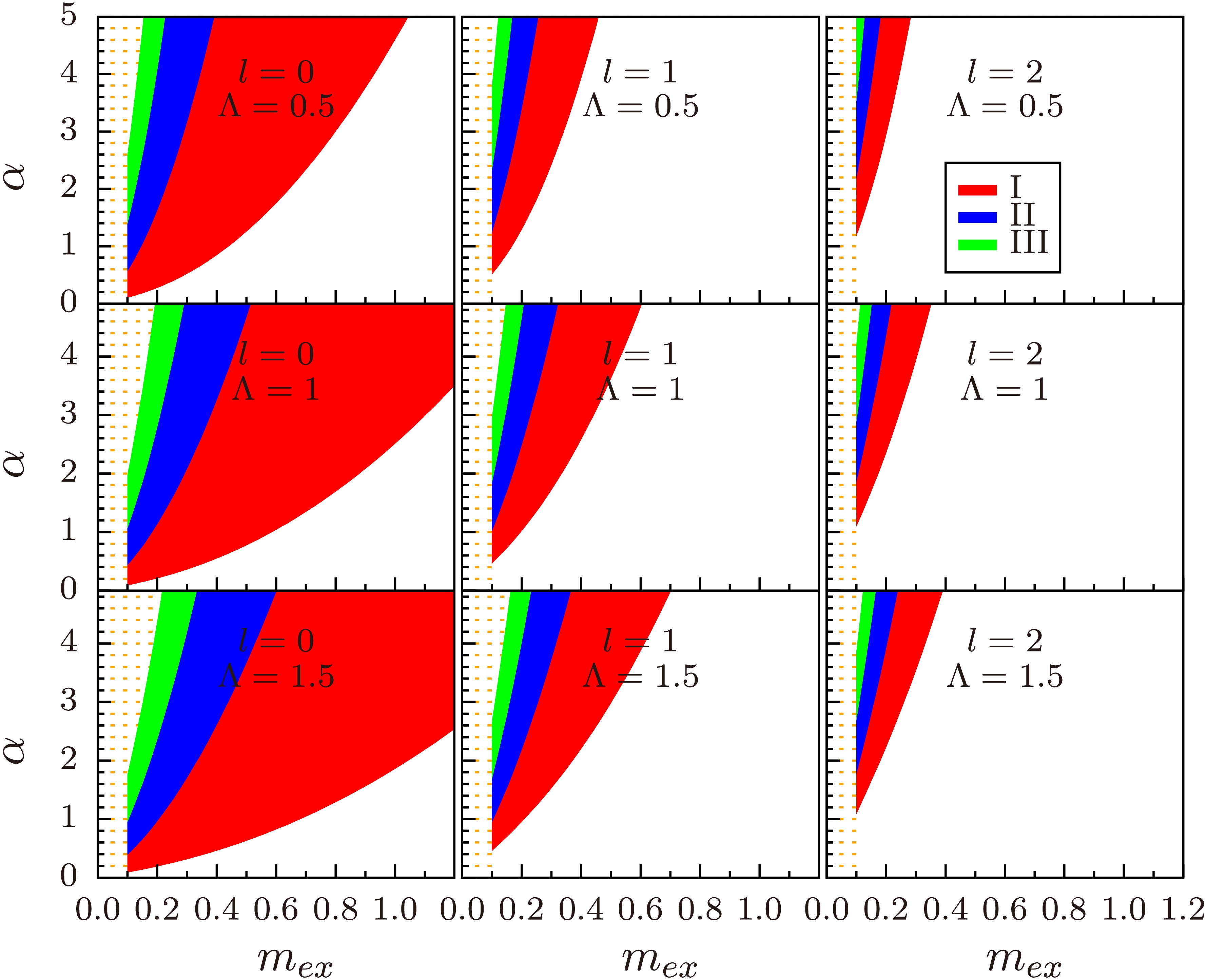
Figure 4. (color online) Critical boundaries for the number of bound states as functions of α and
$ m_{ex} $ for a given angular momentum l and cutoff Λ in the$ V_2(r) $ case, with μ fixed at$ 1 $ . The panels, from left to right, show the cases$ l=0 $ ,$ l=1 $ , and$ l=2 $ . The red (I), blue (II), and green (III) regions indicate the existence of one, two, and three bound states, respectively.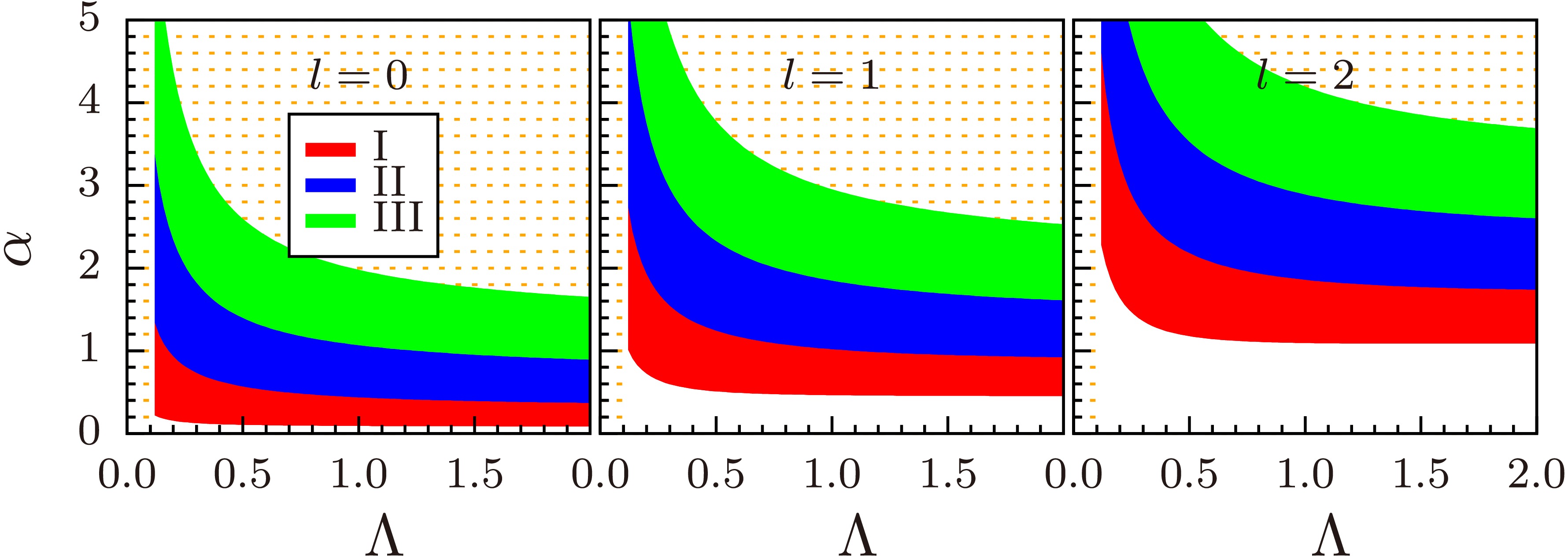
Figure 5. (color online) Critical boundaries for the number of bound states as functions of α and Λ for specific angular momentum l in the
$ V_2(r) $ case, with μ fixed at$ 1 $ and$ m_{ex} $ fixed at$ 0.1 $ . The panels, ordered from left to right, correspond to$ l=0 $ ,$ l=1 $ , and$ l=2 $ . The red (I), blue (II), and green (III) regions indicate the existence of one, two, and three bound states, respectively. -
As in the previous subsection, we use the dipole form factor with the same cutoff,
$ \Lambda = 1 $ . Table 9 shows that the critical values of$ m_{\rm ex} $ are smaller than those in Table 7. This is expected because, for a given nominal cutoff, the strength and range of the effective interaction depend on whether a monopole or dipole form factor is adopted.n l 0 1 1 0.58558680838334368160717264884765735 – 2 0.18270070240342597051691912003895539 0.19689682790771643103189361708297792 3 0.095030571470798752697956881977611261 0.098383578056817713416914243429592524 4 0.058534282044609208097652179586460915 0.060272223040655954415361979835410004 5 0.039695180641185519311747813053258091 0.040805728711342126763446926499838344 Table 9. The critical values of
$ m_{\rm ex} $ for$ \mu=1 $ ,$ \alpha=1 $ , and$ \Lambda=1 $ , categorized by the quantum numbers n and l in the$ V_2(r) $ case.Figure 4 shows that the dependence of α on
$ m_{\rm ex} $ is similar to that in Fig. 2, while Fig. 5 closely parallels Fig. 3 for the dependence of α on Λ. In addition, for the dipole form factor with the same Λ, a smaller$ m_{\rm ex} $ and a larger coupling α are required for bound states to appear. By readjusting Λ, similar critical values can be reproduced within our framework.
Figure 4. (color online) Critical boundaries for the number of bound states as functions of α and
$ m_{\rm ex} $ for a given angular momentum l and cutoff Λ in the$ V_2(r) $ case, with μ fixed at$ 1 $ . The panels, from left to right, show the cases$ l=0 $ ,$ l=1 $ , and$ l=2 $ . The red (I), blue (II), and green (III) regions indicate the existence of one, two, and three bound states, respectively.
Figure 5. (color online) Critical boundaries for the number of bound states as functions of α and Λ for specific angular momentum l in the
$ V_2(r) $ case, with μ fixed at$ 1 $ and$ m_{\rm ex} $ fixed at$ 0.1 $ . The panels, ordered from left to right, correspond to$ l=0 $ ,$ l=1 $ , and$ l=2 $ . The red (I), blue (II), and green (III) regions indicate the existence of one, two, and three bound states, respectively. -
As in the previous subsection, we use the dipole form factor with the same cutoff,
$ \Lambda = 1 $ . Table 9 shows that the critical values of$ m_{\rm ex} $ are smaller than those in Table 7. This is expected because, for a given nominal cutoff, the strength and range of the effective interaction depend on whether a monopole or dipole form factor is adopted.n l 0 1 1 0.58558680838334368160717264884765735 – 2 0.18270070240342597051691912003895539 0.19689682790771643103189361708297792 3 0.095030571470798752697956881977611261 0.098383578056817713416914243429592524 4 0.058534282044609208097652179586460915 0.060272223040655954415361979835410004 5 0.039695180641185519311747813053258091 0.040805728711342126763446926499838344 Table 9. The critical values of
$ m_{\rm ex} $ for$ \mu=1 $ ,$ \alpha=1 $ , and$ \Lambda=1 $ , categorized by the quantum numbers n and l in the$ V_2(r) $ case.Figure 4 shows that the dependence of α on
$ m_{\rm ex} $ is similar to that in Fig. 2, while Fig. 5 closely parallels Fig. 3 for the dependence of α on Λ. In addition, for the dipole form factor with the same Λ, a smaller$ m_{\rm ex} $ and a larger coupling α are required for bound states to appear. By readjusting Λ, similar critical values can be reproduced within our framework.
Figure 4. (color online) Critical boundaries for the number of bound states as functions of α and
$ m_{\rm ex} $ for a given angular momentum l and cutoff Λ in the$ V_2(r) $ case, with μ fixed at$ 1 $ . The panels, from left to right, show the cases$ l=0 $ ,$ l=1 $ , and$ l=2 $ . The red (I), blue (II), and green (III) regions indicate the existence of one, two, and three bound states, respectively.
Figure 5. (color online) Critical boundaries for the number of bound states as functions of α and Λ for specific angular momentum l in the
$ V_2(r) $ case, with μ fixed at$ 1 $ and$ m_{\rm ex} $ fixed at$ 0.1 $ . The panels, ordered from left to right, correspond to$ l=0 $ ,$ l=1 $ , and$ l=2 $ . The red (I), blue (II), and green (III) regions indicate the existence of one, two, and three bound states, respectively. -
In this subsection, we extend the preceding discussion to the
$ D\bar{D} $ system. The kernels$ K_{D\bar{D}} $ and the potential$ V_{D\bar{D}} $ introduced below follow Ref. [48] for the$ J=0 $ $ D\bar{D} $ channel; they should not be confused with the dipole form-factor potential denoted by$ V_2(r) $ in Sec. III.C. The energy spectrum of this system was studied in Ref. [48], where the corresponding potential in the Schrödinger equation for the$ J=0 $ state is given as follows:$ \begin{aligned}[b] K_{D\bar{D}}(\boldsymbol{q})=\;&{\rm i}g^2\left[\frac{3}{4}\bar{K}(\boldsymbol{q},m_\rho)+ \frac{1}{4}\bar{K}(\boldsymbol{q},m_\omega)\right]\\&+{\rm i}g^2_{\sigma}\bar{K}(\boldsymbol{q},m_{\sigma}), \end{aligned} $
(24) $ \begin{aligned}[b] V_{D\bar{D}}(r) =\;&-4\pi\alpha\left[\frac{3}{4}\bar{V}(r,m_\rho)+\frac{1}{4}\bar{V}(r,m_\omega)\right]\\&-{4\pi}\alpha_{\sigma} \bar{V}(r,m_{\sigma}), \end{aligned} $
(25) where
$ \alpha \equiv \dfrac{g^2}{4\pi} $ ,$ \alpha_{\sigma} \equiv \dfrac{g_{\sigma}^2}{4\pi} $ , and$ \bar{K}(\boldsymbol{q},m_{\rm ex})=\frac{1}{\boldsymbol{q}^2+m_{\rm ex}^2} \left(\frac{\Lambda^2-m_{\rm ex}^2}{\Lambda^2+\boldsymbol{q}^2}\right)^2, $
(26) $ \bar{V}(r,m_{\rm ex}) =\frac{1}{8\pi r} \Big[2{\rm e}^{-m_{\rm ex}r}-2{\rm e}^{-\Lambda r}+ {\rm e}^{-\Lambda r}\frac{(m_{\rm ex}^2-\Lambda^2)r}{\Lambda} \Big]. $
(27) We note that the form factor used here is not the dipole form but rather the specific form adopted in Ref. [48].
In Ref. [48], the coupling constants are taken to be
$ g_{\sigma}=-0.76 $ and$ g=5.247 $ (or$ \alpha=2.19 $ and$ \alpha_{\sigma}=0.046 $ ). Since$ \alpha_{\sigma} $ is much smaller than α, we fix its value in the following discussion to study the effects of α and Λ. The masses of the exchanged bosons are taken to be$ m_\rho=0.776 $ GeV,$ m_\omega=0.783 $ GeV, and$ m_\sigma=0.6 $ GeV. The masses of D and$ \bar{D} $ are taken to be$ m_D=m_{\bar{D}}=1.867 $ GeV.In Fig. 6, we show the critical boundaries for the number of bound states as functions of α and Λ, using the same notation as in Fig. 1. For comparison, the parameters used in Ref. [48] are also indicated by the two black triangles, which correspond to
$ \alpha=2.191 $ with$ \Lambda=1.46 $ GeV and$ \Lambda=1.76 $ GeV.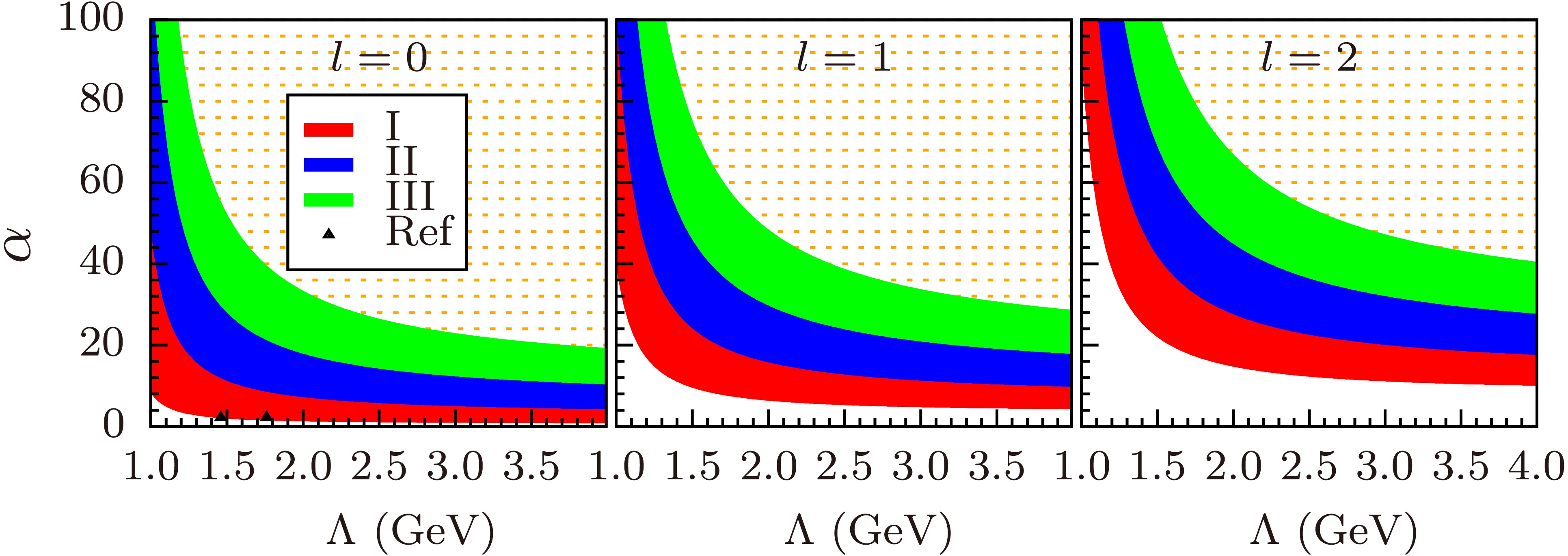
Figure 6. (color online) Critical boundaries indicating the number of bound states as functions of α and Λ for specified angular momentum l in the
$ D\bar{D} $ system. The panels, from left to right, show the cases for$ l=0 $ ,$ l=1 $ , and$ l=2 $ . The red (I), blue (II), and green (III) regions indicate the existence of one, two, and three bound states, respectively.The results in Fig. 6 suggest that the critical value of α for the ground state depends only weakly on Λ when
$ \Lambda>2 $ GeV. To illustrate this behavior in detail, Table 10 lists the corresponding values. These results show that the variation of α with Λ is much milder for$ \Lambda\in[2, 4] $ GeV than for$ \Lambda\in[1, 2] $ GeV.Λ $ \alpha(l=0,n=1) $ $ \alpha(l=0,n=2) $ $ \alpha(l=0,n=3) $ $ \alpha(l=0,n=4) $ 1.0 8.302 48.526 121.416 226.849 1.5 1.927 11.241 28.044 52.311 2.0 1.257 7.216 17.920 33.361 2.5 1.025 5.758 14.240 26.476 3.0 0.910 5.003 12.336 22.918 3.5 0.843 4.538 11.166 20.736 4.0 0.799 4.220 10.371 19.252 Table 10. Critical values of α as functions of Λ for the
$ l=0 $ state in the$ D\bar{D} $ system.Figure 7 shows the number of bound states N as a function of Λ for
$ \alpha=2.191 $ , 5, 10, and 20. For coupling strengths typical of the present phenomenological context, N remains equal to 1 for$ \Lambda>1.4 $ GeV. For$ \alpha=5 $ , N also remains equal to 1 for$ \Lambda>1.1 $ GeV. For larger values of α, N increases with Λ.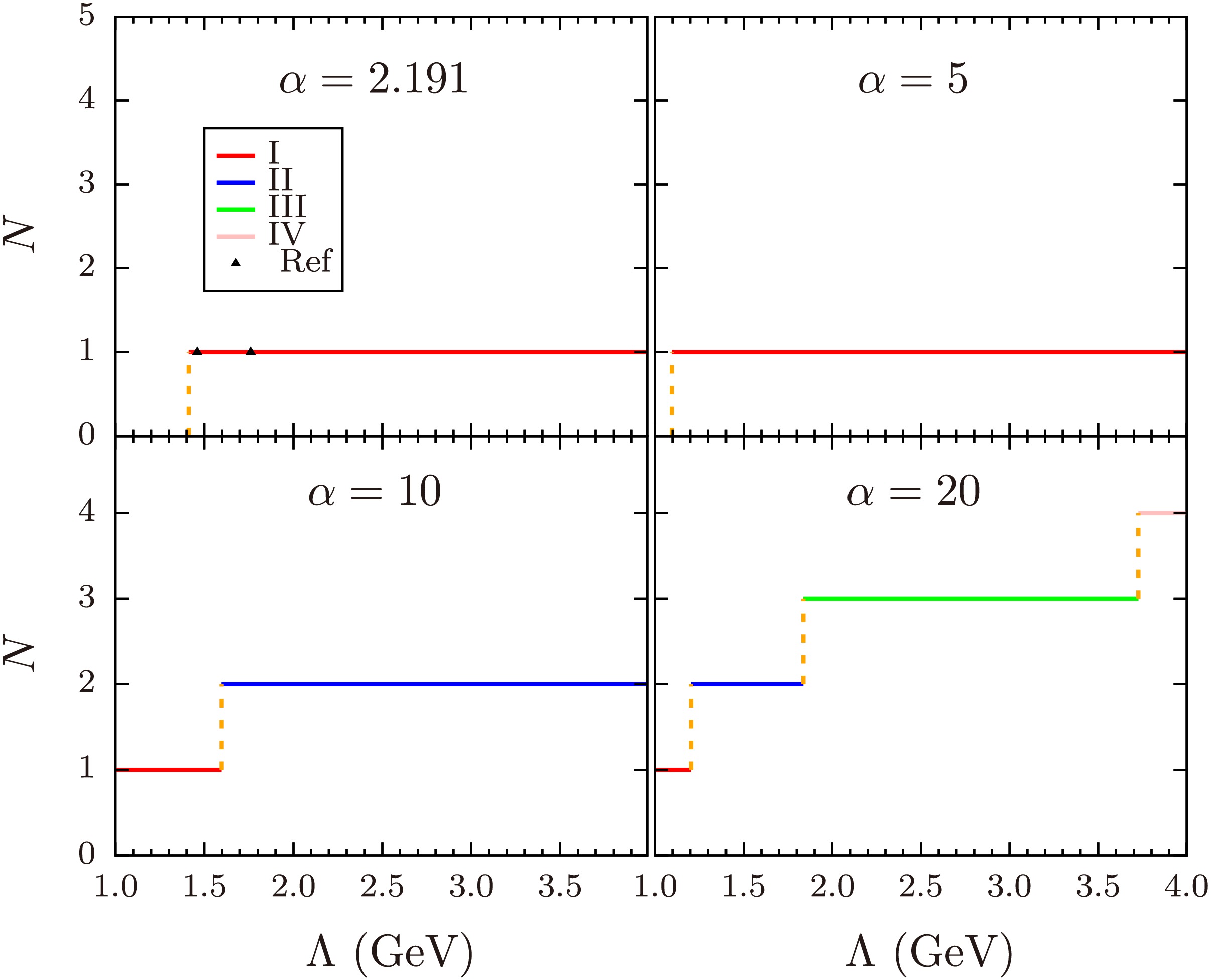
Figure 7. (color online) Number of bound states N as a function of Λ for selected values of α at
$ l=0 $ in the$ D\bar{D} $ system.In Fig. 8, we show the binding energy
$ E_b $ as a function of the coupling constant α for fixed Λ in the$ l=0 $ case. The parameters used in Ref. [48] are also indicated by the two black triangles. The notations$ 1^{\text{st}} $ ,$ 2^{\text{nd}} $ , and$ 3^{\text{rd}} $ refer to the first, second, and third bound states with$ l=0 $ , respectively. The results show that$ E_b $ is nearly linear in α. As α increases, additional bound states appear, demonstrating that the magnitude of the coupling constant plays a critical role in determining the number of bound states at a fixed cutoff Λ.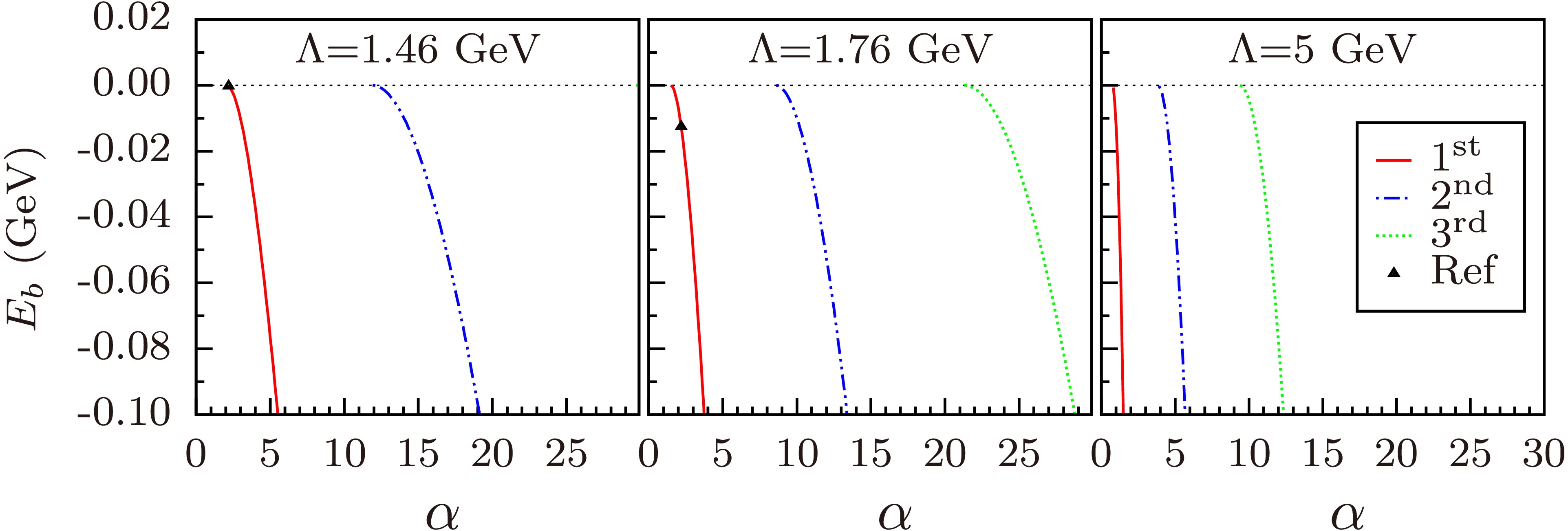
Figure 8. (color online) The binding energy
$ E_b $ as a function of α for fixed Λ in the$ l=0 $ case of the$ D\bar{D} $ system. The panels, ordered from left to right, show the cases for$ \Lambda=1.46 $ GeV,$ \Lambda=1.76 $ GeV, and$ \Lambda=5 $ GeV. The red, blue, and green lines denote the first, second, and third bound states, respectively. The two black triangles correspond to the results obtained using the parameters given in Ref. [48].In Fig. 9, we show the binding energy
$ E_b $ as a function of the cutoff Λ for fixed coupling constant α and angular momentum l. The results indicate that$ E_b $ is nearly linear with respect to the cutoff Λ at large Λ. When α is fixed at$ 2.19 $ (the value used in Ref. [48]), only one bound state is obtained.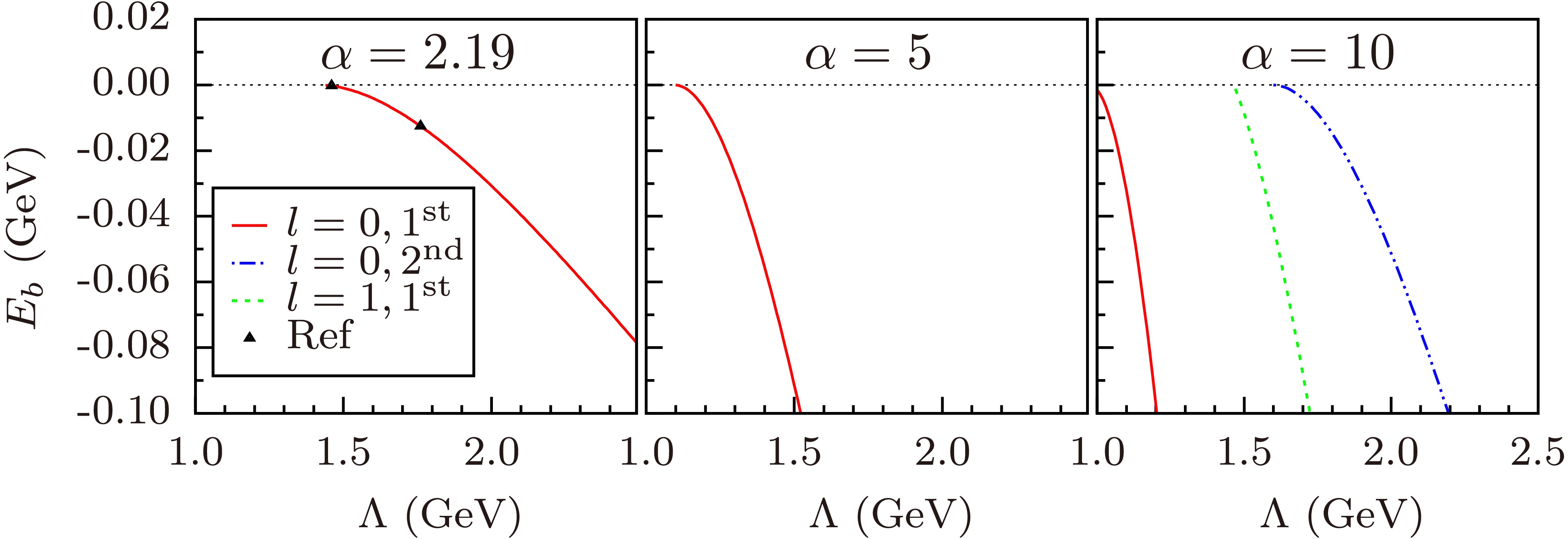
Figure 9. (color online) Binding energy
$ E_b $ as a function of Λ for fixed angular momentum l and coupling constant α in the$ D\bar{D} $ system. The panels, ordered from left to right, show the cases for$ \alpha=2.19 $ ,$ \alpha=5 $ , and$ \alpha=10 $ . The red, blue, and green lines denote the first bound state with$ l=0 $ , the second bound state with$ l=0 $ , and the first bound state with$ l=1 $ , respectively. The black triangle indicates the results obtained using the parameters given in Ref. [48].For comparison, we apply the same interaction parameters directly to the
$ B\bar{B} $ system. The corresponding results for the number of bound states N are shown in Fig. 10 and exhibit trends similar to those in the$ D\bar{D} $ case.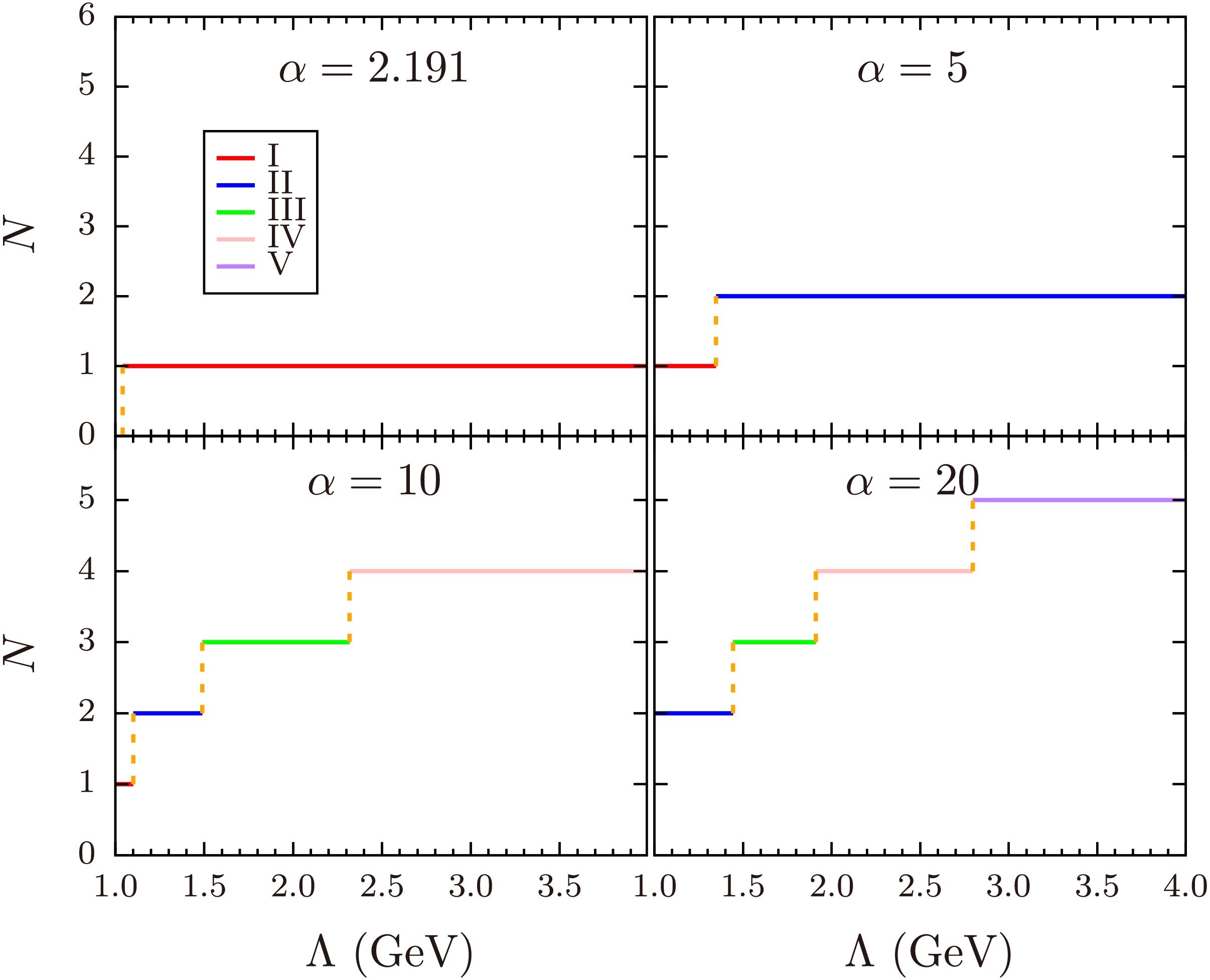
Figure 10. (color online) The number of bound states N as a function of Λ for selected values of α at
$ l=0 $ in the$ B\bar{B} $ system, with the interaction parameters taken from the$ D\bar{D} $ analysis as a test.Taken together, these results indicate that the existence and multiplicity of bound states are strongly correlated with the coupling constant α, particularly when α is small, but depend only weakly on the cutoff Λ over a broad region.
-
In this subsection, we extend the preceding discussion to the
$ D\bar{D} $ system. The kernels$ K_{D\bar{D}} $ and the potential$ V_{D\bar{D}} $ introduced below follow Ref. [48] for the$ J=0 $ $ D\bar{D} $ channel; they should not be confused with the dipole form-factor potential denoted by$ V_2(r) $ in Sec. 3.3. The energy spectrum of this system was studied in Ref. [48], where the corresponding potential in the Schrödinger equation for the$ J=0 $ state is given as follows:$ \begin{aligned}[b] K_{D\bar{D}}(\boldsymbol{q})=\;&ig^2\left[\frac{3}{4}\bar{K}(\boldsymbol{q},m_\rho)+ \frac{1}{4}\bar{K}(\boldsymbol{q},m_\omega)\right]\\&+ig^2_{\sigma}\bar{K}(\boldsymbol{q},m_{\sigma}), \end{aligned} $
(24) $ \begin{aligned}[b] V_{D\bar{D}}(r) =\;&-4\pi\alpha\left[\frac{3}{4}\bar{V}(r,m_\rho)+\frac{1}{4}\bar{V}(r,m_\omega)\right]\\&-{4\pi}\alpha_{\sigma} \bar{V}(r,m_{\sigma}), \end{aligned} $
(25) where
$ \alpha \equiv \dfrac{g^2}{4\pi} $ ,$ \alpha_{\sigma} \equiv \dfrac{g_{\sigma}^2}{4\pi} $ , and$ \bar{K}(\boldsymbol{q},m_{ex})=\frac{1}{\boldsymbol{q}^2+m_{ex}^2} \left(\frac{\Lambda^2-m_{ex}^2}{\Lambda^2+\boldsymbol{q}^2}\right)^2, $
(26) $ \bar{V}(r,m_{ex}) =\frac{1}{8\pi r} \Big[2e^{-m_{ex}r}-2e^{-\Lambda r}+ e^{-\Lambda r}\frac{(m_{ex}^2-\Lambda^2)r}{\Lambda} \Big]. $
(27) We note that the form factor used here is not the dipole form but rather the specific form adopted in Ref. [48].
In Ref. [48], the coupling constants are taken to be
$ g_{\sigma}=-0.76 $ and$ g=5.247 $ (or$ \alpha=2.19 $ and$ \alpha_{\sigma}=0.046 $ ). Since$ \alpha_{\sigma} $ is much smaller than α, we fix its value in the following discussion to study the effects of α and Λ. The masses of the exchanged bosons are taken to be$ m_\rho=0.776 $ GeV,$ m_\omega=0.783 $ GeV, and$ m_\sigma=0.6 $ GeV. The masses of D and$ \bar{D} $ are taken to be$ m_D=m_{\bar{D}}=1.867 $ GeV.In Fig. 6, we show the critical boundaries for the number of bound states as functions of α and Λ, using the same notation as in Fig. 1. For comparison, the parameters used in Ref. [48] are also indicated by the two black triangles, which correspond to
$ \alpha=2.191 $ with$ \Lambda=1.46 $ GeV and$ \Lambda=1.76 $ GeV.
Figure 6. (color online) Critical boundaries indicating the number of bound states as functions of α and Λ for specified angular momentum l in the
$ D\bar{D} $ system. The panels, from left to right, show the cases for$ l=0 $ ,$ l=1 $ , and$ l=2 $ . The red (I), blue (II), and green (III) regions indicate the existence of one, two, and three bound states, respectively.The results in Fig. 6 suggest that the critical value of α for the ground state depends only weakly on Λ when
$ \Lambda>2 $ GeV. To illustrate this behavior in detail, Table 10 lists the corresponding values. These results show that the variation of α with Λ is much milder for$ \Lambda\in[2, 4] $ GeV than for$ \Lambda\in[1, 2] $ GeV.Λ $ \alpha(l=0,n=1) $ $ \alpha(l=0,n=2) $ $ \alpha(l=0,n=3) $ $ \alpha(l=0,n=4) $ 1.0 8.302 48.526 121.416 226.849 1.5 1.927 11.241 28.044 52.311 2.0 1.257 7.216 17.920 33.361 2.5 1.025 5.758 14.240 26.476 3.0 0.910 5.003 12.336 22.918 3.5 0.843 4.538 11.166 20.736 4.0 0.799 4.220 10.371 19.252 Table 10. Critical values of α as functions of Λ for the
$ l=0 $ state in the$ D\bar{D} $ system.Figure 7 shows the number of bound states N as a function of Λ for
$ \alpha=2.191 $ , 5, 10, and 20. For coupling strengths typical of the present phenomenological context, N remains equal to 1 for$ \Lambda>1.4 $ GeV. For$ \alpha=5 $ , N also remains equal to 1 for$ \Lambda>1.1 $ GeV. For larger values of α, N increases with Λ.
Figure 7. (color online) Number of bound states N as a function of Λ for selected values of α at
$ l=0 $ in the$ D\bar{D} $ system.In Fig. 8, we show the binding energy
$ E_b $ as a function of the coupling constant α for fixed Λ in the$ l=0 $ case. The parameters used in Ref. [48] are also indicated by the two black triangles. The notations$ 1^{\text{st}} $ ,$ 2^{\text{nd}} $ , and$ 3^{\text{rd}} $ refer to the first, second, and third bound states with$ l=0 $ , respectively. The results show that$ E_b $ is nearly linear in α. As α increases, additional bound states appear, demonstrating that the magnitude of the coupling constant plays a critical role in determining the number of bound states at a fixed cutoff Λ.
Figure 8. (color online) The binding energy
$ E_b $ as a function of α for fixed Λ in the$ l=0 $ case of the$ D\bar{D} $ system. The panels, ordered from left to right, show the cases for$ \Lambda=1.46 $ GeV,$ \Lambda=1.76 $ GeV, and$ \Lambda=5 $ GeV. The red, blue, and green lines denote the first, second, and third bound states, respectively. The two black triangles correspond to the results obtained using the parameters given in Ref. [48].In Fig. 9, we show the binding energy
$ E_b $ as a function of the cutoff Λ for fixed coupling constant α and angular momentum l. The results indicate that$ E_b $ is nearly linear with respect to the cutoff Λ at large Λ. When α is fixed at$ 2.19 $ (the value used in Ref. [48]), only one bound state is obtained.
Figure 9. (color online) Binding energy
$ E_b $ as a function of Λ for fixed angular momentum l and coupling constant α in the$ D\bar{D} $ system. The panels, ordered from left to right, show the cases for$ \alpha=2.19 $ ,$ \alpha=5 $ , and$ \alpha=10 $ . The red, blue, and green lines denote the first bound state with$ l=0 $ , the second bound state with$ l=0 $ , and the first bound state with$ l=1 $ , respectively. The black triangle indicates the results obtained using the parameters given in Ref. [48].For comparison, we apply the same interaction parameters directly to the
$ B\bar{B} $ system. The corresponding results for the number of bound states N are shown in Fig. 10 and exhibit trends similar to those in the$ D\bar{D} $ case.
Figure 10. (color online) The number of bound states N as a function of Λ for selected values of α at
$ l=0 $ in the$ B\bar{B} $ system, with the interaction parameters taken from the$ D\bar{D} $ analysis as a test.Taken together, these results indicate that the existence and multiplicity of bound states are strongly correlated with the coupling constant α, particularly when α is small, but depend only weakly on the cutoff Λ over a broad region.
-
In this subsection, we extend the preceding discussion to the
$ D\bar{D} $ system. The kernels$ K_{D\bar{D}} $ and the potential$ V_{D\bar{D}} $ introduced below follow Ref. [48] for the$ J=0 $ $ D\bar{D} $ channel; they should not be confused with the dipole form-factor potential denoted by$ V_2(r) $ in Sec. III.C. The energy spectrum of this system was studied in Ref. [48], where the corresponding potential in the Schrödinger equation for the$ J=0 $ state is given as follows:$ \begin{aligned}[b] K_{D\bar{D}}(\boldsymbol{q})=\;&{\rm i}g^2\left[\frac{3}{4}\bar{K}(\boldsymbol{q},m_\rho)+ \frac{1}{4}\bar{K}(\boldsymbol{q},m_\omega)\right]\\&+{\rm i}g^2_{\sigma}\bar{K}(\boldsymbol{q},m_{\sigma}), \end{aligned} $
(24) $ \begin{aligned}[b] V_{D\bar{D}}(r) =\;&-4\pi\alpha\left[\frac{3}{4}\bar{V}(r,m_\rho)+\frac{1}{4}\bar{V}(r,m_\omega)\right]\\&-{4\pi}\alpha_{\sigma} \bar{V}(r,m_{\sigma}), \end{aligned} $
(25) where
$ \alpha \equiv \dfrac{g^2}{4\pi} $ ,$ \alpha_{\sigma} \equiv \dfrac{g_{\sigma}^2}{4\pi} $ , and$ \bar{K}(\boldsymbol{q},m_{\rm ex})=\frac{1}{\boldsymbol{q}^2+m_{\rm ex}^2} \left(\frac{\Lambda^2-m_{\rm ex}^2}{\Lambda^2+\boldsymbol{q}^2}\right)^2, $
(26) $ \bar{V}(r,m_{\rm ex}) =\frac{1}{8\pi r} \Big[2{\rm e}^{-m_{\rm ex}r}-2{\rm e}^{-\Lambda r}+ {\rm e}^{-\Lambda r}\frac{(m_{\rm ex}^2-\Lambda^2)r}{\Lambda} \Big]. $
(27) We note that the form factor used here is not the dipole form but rather the specific form adopted in Ref. [48].
In Ref. [48], the coupling constants are taken to be
$ g_{\sigma}=-0.76 $ and$ g=5.247 $ (or$ \alpha=2.19 $ and$ \alpha_{\sigma}=0.046 $ ). Since$ \alpha_{\sigma} $ is much smaller than α, we fix its value in the following discussion to study the effects of α and Λ. The masses of the exchanged bosons are taken to be$ m_\rho=0.776 $ GeV,$ m_\omega=0.783 $ GeV, and$ m_\sigma=0.6 $ GeV. The masses of D and$ \bar{D} $ are taken to be$ m_D=m_{\bar{D}}=1.867 $ GeV.In Fig. 6, we show the critical boundaries for the number of bound states as functions of α and Λ, using the same notation as in Fig. 1. For comparison, the parameters used in Ref. [48] are also indicated by the two black triangles, which correspond to
$ \alpha=2.191 $ with$ \Lambda=1.46 $ GeV and$ \Lambda=1.76 $ GeV.
Figure 6. (color online) Critical boundaries indicating the number of bound states as functions of α and Λ for specified angular momentum l in the
$ D\bar{D} $ system. The panels, from left to right, show the cases for$ l=0 $ ,$ l=1 $ , and$ l=2 $ . The red (I), blue (II), and green (III) regions indicate the existence of one, two, and three bound states, respectively.The results in Fig. 6 suggest that the critical value of α for the ground state depends only weakly on Λ when
$ \Lambda>2 $ GeV. To illustrate this behavior in detail, Table 10 lists the corresponding values. These results show that the variation of α with Λ is much milder for$ \Lambda\in[2, 4] $ GeV than for$ \Lambda\in[1, 2] $ GeV.Λ $ \alpha(l=0,n=1) $ $ \alpha(l=0,n=2) $ $ \alpha(l=0,n=3) $ $ \alpha(l=0,n=4) $ 1.0 8.302 48.526 121.416 226.849 1.5 1.927 11.241 28.044 52.311 2.0 1.257 7.216 17.920 33.361 2.5 1.025 5.758 14.240 26.476 3.0 0.910 5.003 12.336 22.918 3.5 0.843 4.538 11.166 20.736 4.0 0.799 4.220 10.371 19.252 Table 10. Critical values of α as functions of Λ for the
$ l=0 $ state in the$ D\bar{D} $ system.Figure 7 shows the number of bound states N as a function of Λ for
$ \alpha=2.191 $ , 5, 10, and 20. For coupling strengths typical of the present phenomenological context, N remains equal to 1 for$ \Lambda>1.4 $ GeV. For$ \alpha=5 $ , N also remains equal to 1 for$ \Lambda>1.1 $ GeV. For larger values of α, N increases with Λ.
Figure 7. (color online) Number of bound states N as a function of Λ for selected values of α at
$ l=0 $ in the$ D\bar{D} $ system.In Fig. 8, we show the binding energy
$ E_b $ as a function of the coupling constant α for fixed Λ in the$ l=0 $ case. The parameters used in Ref. [48] are also indicated by the two black triangles. The notations$ 1^{\text{st}} $ ,$ 2^{\text{nd}} $ , and$ 3^{\text{rd}} $ refer to the first, second, and third bound states with$ l=0 $ , respectively. The results show that$ E_b $ is nearly linear in α. As α increases, additional bound states appear, demonstrating that the magnitude of the coupling constant plays a critical role in determining the number of bound states at a fixed cutoff Λ.
Figure 8. (color online) The binding energy
$ E_b $ as a function of α for fixed Λ in the$ l=0 $ case of the$ D\bar{D} $ system. The panels, ordered from left to right, show the cases for$ \Lambda=1.46 $ GeV,$ \Lambda=1.76 $ GeV, and$ \Lambda=5 $ GeV. The red, blue, and green lines denote the first, second, and third bound states, respectively. The two black triangles correspond to the results obtained using the parameters given in Ref. [48].In Fig. 9, we show the binding energy
$ E_b $ as a function of the cutoff Λ for fixed coupling constant α and angular momentum l. The results indicate that$ E_b $ is nearly linear with respect to the cutoff Λ at large Λ. When α is fixed at$ 2.19 $ (the value used in Ref. [48]), only one bound state is obtained.
Figure 9. (color online) Binding energy
$ E_b $ as a function of Λ for fixed angular momentum l and coupling constant α in the$ D\bar{D} $ system. The panels, ordered from left to right, show the cases for$ \alpha=2.19 $ ,$ \alpha=5 $ , and$ \alpha=10 $ . The red, blue, and green lines denote the first bound state with$ l=0 $ , the second bound state with$ l=0 $ , and the first bound state with$ l=1 $ , respectively. The black triangle indicates the results obtained using the parameters given in Ref. [48].For comparison, we apply the same interaction parameters directly to the
$ B\bar{B} $ system. The corresponding results for the number of bound states N are shown in Fig. 10 and exhibit trends similar to those in the$ D\bar{D} $ case.
Figure 10. (color online) The number of bound states N as a function of Λ for selected values of α at
$ l=0 $ in the$ B\bar{B} $ system, with the interaction parameters taken from the$ D\bar{D} $ analysis as a test.Taken together, these results indicate that the existence and multiplicity of bound states are strongly correlated with the coupling constant α, particularly when α is small, but depend only weakly on the cutoff Λ over a broad region.
-
In this study, we investigate the critical behavior of bound states in the Yukawa potential and a modified version of it, both of which are widely used in the OBE model for hadronic molecular states. The analysis is based on a highly accurate numerical method. Our numerical result for the critical mass
$ m_{\rm ex} $ of the ground state is consistent with values reported in the literature. Furthermore, our results for the$ l=1 $ case are significantly more precise than previously reported values. For the$ D\bar{D} $ hadronic molecular system, our results indicate that the number of hadronic molecular states is only weakly sensitive to the cutoff Λ over a broad range (for example,$ \alpha\le5 $ and$ \Lambda>1.5\; \mathrm{GeV} $ ), although the binding energies may still depend on Λ, as discussed above. This behavior suggests an interesting global regularity in hadronic molecular states. Finally, this highly accurate numerical method can be straightforwardly applied to higher-l cases or other systems. -
In this study, we investigate the critical behavior of bound states in the Yukawa potential and a modified version of it, both of which are widely used in the OBE model for hadronic molecular states. The analysis is based on a highly accurate numerical method. Our numerical result for the critical mass
$ m_{\rm ex} $ of the ground state is consistent with values reported in the literature. Furthermore, our results for the$ l=1 $ case are significantly more precise than previously reported values. For the$ D\bar{D} $ hadronic molecular system, our results indicate that the number of hadronic molecular states is only weakly sensitive to the cutoff Λ over a broad range (for example,$ \alpha\le5 $ and$ \Lambda>1.5\; \mathrm{GeV} $ ), although the binding energies may still depend on Λ, as discussed above. This behavior suggests an interesting global regularity in hadronic molecular states. Finally, this highly accurate numerical method can be straightforwardly applied to higher-l cases or other systems. -
In this study, we investigate the critical behavior of bound states in the Yukawa potential and a modified version of it, both of which are widely used in the OBE model for hadronic molecular states. The analysis is based on a highly accurate numerical method. Our numerical result for the critical mass
$ m_{ex} $ of the ground state is consistent with values reported in the literature. Furthermore, our results for the$ l=1 $ case are significantly more precise than previously reported values. For the$ D\bar{D} $ hadronic molecular system, our results indicate that the number of hadronic molecular states is only weakly sensitive to the cutoff Λ over a broad range (for example,$ \alpha\le5 $ and$ \Lambda>1.5\; \mathrm{GeV} $ ), although the binding energies may still depend on Λ, as discussed above. This behavior suggests an interesting global regularity in hadronic molecular states. Finally, this highly accurate numerical method can be straightforwardly applied to higher-l cases or other systems.
Critical properties of bound states with one-boson-exchange potential
- Received Date: 2026-04-11
- Available Online: 2026-09-15
Abstract: In this study, we discuss general critical properties of bound states with a one-boson-exchange potential. For simplicity, we first consider a system of two identical scalar particles as an example. The interaction between these two scalar particles is described by the exchange of another massive scalar meson under the instantaneous approximation, which yields the Yukawa potential. A highly accurate numerical method is used to determine the critical mass of the system. The resulting critical mass for the ground state is consistent with values reported in the literature, agreeing to about 35 significant figures. Highly accurate results for the $l=1$ case are also presented, which are significantly more precise than those previously reported in the literature. Furthermore, we extend the discussion to physical hadronic molecular states, for which form factors are introduced in the interaction to describe the structure of hadrons. Our numerical results show that although the binding energies of the hadronic molecular states depend on the cutoff in the form factors, the number of hadronic molecular states is almost independent of the cutoffs over a very wide physically relevant range. This indicates a strong and important property: for physically small couplings, the number of hadronic molecular states is almost solely determined by the coupling constants and the masses of the exchange particles. This highly accurate numerical method can also be straightforwardly applied to higher l cases or other systems.



 DownLoad: