


 Abstract
 HTML
HTML Reference
 Related
 PDF
PDF


-
Since 2019, the Event Horizon Telescope (EHT) international collaboration has released images of the supermassive black holes at the centers of the radio galaxy M87* and of our Galaxy, SgrA* [1, 2], marking a new era in black hole physics. Both images exhibit similar structures: a bright, asymmetric ring surrounding a central region of diminished intensity. According to General Relativity (GR), a thin, bright photon ring—predicted theoretically but not yet directly observed by the EHT—is hidden within the bright emission ring, while the central dark region represents the black hole shadow [3]. When the accretion flow extends to the event horizon, the dark region corresponds to the inner shadow of the black hole, i.e., the direct projection of the event horizon onto the observer's screen. Its existence arises from the horizon itself, rather than from light rays being captured by the gravitational field. The shadow forms because light rays passing near the black hole are captured by its strong gravitational field and cannot reach the observer, thereby creating a dark region on the image plane [3]. The shadow image encodes valuable information about the spacetime geometry, accretion processes, and the surrounding matter distribution [4−6]. Consequently, it provides an unprecedented opportunity to test GR in the strong-field regime and to probe the complex plasma environment around compact objects [7]. Hence, constructing theoretical models of black hole shadows consistent with observational images has become one of the frontiers of contemporary black hole physics [8].
Supermassive black holes accrete hot, magnetized plasma, forming luminous accretion disks. Furthermore, for highly spinning black holes, electromagnetic energy can drive relativistic jets [9]. In theory, both the accretion disk and the jet can serve as light sources for generating black hole shadow images. In 1973, Shakura and Sunyaev first proposed the geometrically thin and optically thick standard accretion disk model [10]. Subsequently, in 1974, by incorporating the relativistic effects of matter motion near black holes [11], the Shapiro–Lightman–Eardley model was introduced, assuming that the accretion disk is both geometrically and optically thin. By studying the optical appearance of a black hole surrounded by a thin accretion disk, Jean-Pierre Luminet demonstrated in 1979 that the critical curve of a Schwarzschild black hole remains a perfect circle for any viewing angle [12]. Later, shadow images of black holes with Keplerian accretion disks in Kerr spacetime were also investigated [13]. In recent years, spherical accretion models [14−16], optically and geometrically thin disk models [17−21], and geometrically thick disk models [22−24] have all been extensively discussed. The observational achievements of the EHT have brought black hole shadow research into a new stage. Based on the EHT data, numerous studies have focused on constraining the parameters of various black hole models [25, 26]. Meanwhile, related topics such as hot spot images [27], polarized images [28−30], jet images [23], and boson star images [26, 31] have also attracted widespread interest.
In the study of black hole images, polarization images play a crucial role. By comparing theoretically predicted polarization images with observational data, one can gain deeper insights into the astrophysical properties of accretion flows [32]. For a Schwarzschild black hole background, the EHT collaboration successfully reproduced the observed polarization image of M87* by employing the analytical approximation of light rays derived by Beloborodov [33, 34]. This approach was later extended to the Kerr black hole. Gelles et al. constructed a simplified model with an equatorial emission source and produced the corresponding polarization image [35]. These studies suggest that polarization characteristics are governed not only by magnetic fields but also by black hole spacetime parameters and the observation inclination angle. Beyond the Schwarzschild and Kerr black holes, the polarization images of other black hole types and horizonless ultra-compact objects have also been widely investigated, yielding a series of important results [36−38].
Motivated by these developments, it is therefore important to further explore the shadow and polarization images of black holes in alternative gravitational theories. Such studies may provide new theoretical templates for future high-resolution observations and offer additional avenues for testing the nature of strong-field gravity. Among various modified gravity theories, Einstein–Gauss–Bonnet (EGB) gravity provides a particularly well-motivated framework to investigate gravitational phenomena beyond general relativity. It is widely recognized that the uniqueness of the Einstein field equations is established by Lovelock's theorem [39]. However, in higher-dimensional spacetimes (
$ D \gt 4 $ ), the Einstein–Hilbert action is no longer unique. A prominent example is EGB gravity, whose theoretical origin lies in heterotic string theory [40, 41]. EGB gravity has attracted extensive attention because it not only represents the low-energy limit of string theory [42] but also gives rise to ghost-free, nontrivial gravitational self-interactions [43]. Within this framework, one can explore fundamental problems of gravitation in a broader theoretical context than that of GR [44]. The spherically symmetric and static black hole solution in EGB theory was first proposed by Boulware and Deser [45], and subsequently, various interesting black hole solutions have been obtained for different matter sources [46−49]. For spherically symmetric black holes, the observable features under spherical accretion have been analyzed, and the influence of the GB parameter on the black hole shadow has been explored [15]. However, the observable features of rotating EGB black holes, particularly their shadow and polarization images, still await systematic investigation. To this end, we strategically adopt an optically thin and geometrically thin accretion disk as the emission source model, aiming to reveal the unique spacetime characteristics of EGB gravity through precise numerical simulations of the black hole shadow images. Furthermore, the polarization structure of rotating EGB black holes has not yet been explored. An in-depth study of their polarization images, combined with accretion disk imaging, may not only provide theoretical grounds for testing the validity of EGB gravity but also offer key observational criteria for distinguishing EGB gravity from general relativity. This paper aims to provide a systematic theoretical analysis of the observational features of rotating EGB black holes.The structure of this paper is organized as follows. In Sec. II, we briefly review the exact solution of the rotating EGB black hole and present the equations of null geodesics. Section III introduces the ray-tracing techniques and the camera projection method. In Secs. IV and V, we investigate the shadow and polarization images of the rotating EGB black hole illuminated by a thin accretion disk. Finally, Sec. VI provides the conclusion and discussion. Throughout this work, we adopt geometrized units with
$ c = G = 1 $ , where c and G denote the speed of light in vacuum and the gravitational constant, respectively. -
Since 2019, the Event Horizon Telescope (EHT) international collaboration has released images of the supermassive black holes at the centers of the radio galaxy M87* and of our Galaxy, SgrA* [1, 2], marking a new era in black hole physics. Both images exhibit similar structures: a bright, asymmetric ring surrounding a central region of diminished intensity. According to General Relativity (GR), a thin, bright photon ring—predicted theoretically but not yet directly observed by the EHT—is hidden within the bright emission ring, while the central dark region represents the black hole shadow [3]. When the accretion flow extends to the event horizon, the dark region corresponds to the inner shadow of the black hole, i.e., the direct projection of the event horizon onto the observer's screen. Its existence arises from the horizon itself, rather than from light rays being captured by the gravitational field. The shadow forms because light rays passing near the black hole are captured by its strong gravitational field and cannot reach the observer, thereby creating a dark region on the image plane [3]. The shadow image encodes valuable information about the spacetime geometry, accretion processes, and the surrounding matter distribution [4−6]. Consequently, it provides an unprecedented opportunity to test GR in the strong-field regime and to probe the complex plasma environment around compact objects [7]. Hence, constructing theoretical models of black hole shadows consistent with observational images has become one of the frontiers of contemporary black hole physics [8].
Supermassive black holes accrete hot, magnetized plasma, forming luminous accretion disks. Furthermore, for highly spinning black holes, electromagnetic energy can drive relativistic jets [9]. In theory, both the accretion disk and the jet can serve as light sources for generating black hole shadow images. In 1973, Shakura and Sunyaev first proposed the geometrically thin and optically thick standard accretion disk model [10]. Subsequently, in 1974, by incorporating the relativistic effects of matter motion near black holes [11], the Shapiro–Lightman–Eardley model was introduced, assuming that the accretion disk is both geometrically and optically thin. By studying the optical appearance of a black hole surrounded by a thin accretion disk, Jean-Pierre Luminet demonstrated in 1979 that the critical curve of a Schwarzschild black hole remains a perfect circle for any viewing angle [12]. Later, shadow images of black holes with Keplerian accretion disks in Kerr spacetime were also investigated [13]. In recent years, spherical accretion models [14−16], optically and geometrically thin disk models [17−21], and geometrically thick disk models [22−24] have all been extensively discussed. The observational achievements of the EHT have brought black hole shadow research into a new stage. Based on the EHT data, numerous studies have focused on constraining the parameters of various black hole models [25, 26]. Meanwhile, related topics such as hot spot images [27], polarized images [28−30], jet images [23], and boson star images [26, 31] have also attracted widespread interest.
In the study of black hole images, polarization images play a crucial role. By comparing theoretically predicted polarization images with observational data, one can gain deeper insights into the astrophysical properties of accretion flows [32]. For a Schwarzschild black hole background, the EHT collaboration successfully reproduced the observed polarization image of M87* by employing the analytical approximation of light rays derived by Beloborodov [33, 34]. This approach was later extended to the Kerr black hole. Gelles et al. constructed a simplified model with an equatorial emission source and produced the corresponding polarization image [35]. These studies suggest that polarization characteristics are governed not only by magnetic fields but also by black hole spacetime parameters and the observation inclination angle. Beyond the Schwarzschild and Kerr black holes, the polarization images of other black hole types and horizonless ultra-compact objects have also been widely investigated, yielding a series of important results [36−38].
Motivated by these developments, it is therefore important to further explore the shadow and polarization images of black holes in alternative gravitational theories. Such studies may provide new theoretical templates for future high-resolution observations and offer additional avenues for testing the nature of strong-field gravity. Among various modified gravity theories, Einstein–Gauss–Bonnet (EGB) gravity provides a particularly well-motivated framework to investigate gravitational phenomena beyond general relativity. It is widely recognized that the uniqueness of the Einstein field equations is established by Lovelock's theorem [39]. However, in higher-dimensional spacetimes (
$ D \gt 4 $ ), the Einstein–Hilbert action is no longer unique. A prominent example is EGB gravity, whose theoretical origin lies in heterotic string theory [40, 41]. EGB gravity has attracted extensive attention because it not only represents the low-energy limit of string theory [42] but also gives rise to ghost-free, nontrivial gravitational self-interactions [43]. Within this framework, one can explore fundamental problems of gravitation in a broader theoretical context than that of GR [44]. The spherically symmetric and static black hole solution in EGB theory was first proposed by Boulware and Deser [45], and subsequently, various interesting black hole solutions have been obtained for different matter sources [46−49]. For spherically symmetric black holes, the observable features under spherical accretion have been analyzed, and the influence of the GB parameter on the black hole shadow has been explored [15]. However, the observable features of rotating EGB black holes, particularly their shadow and polarization images, still await systematic investigation. To this end, we strategically adopt an optically thin and geometrically thin accretion disk as the emission source model, aiming to reveal the unique spacetime characteristics of EGB gravity through precise numerical simulations of the black hole shadow images. Furthermore, the polarization structure of rotating EGB black holes has not yet been explored. An in-depth study of their polarization images, combined with accretion disk imaging, may not only provide theoretical grounds for testing the validity of EGB gravity but also offer key observational criteria for distinguishing EGB gravity from general relativity. This paper aims to provide a systematic theoretical analysis of the observational features of rotating EGB black holes.The structure of this paper is organized as follows. In Sec. II, we briefly review the exact solution of the rotating EGB black hole and present the equations of null geodesics. Section III introduces the ray-tracing techniques and the camera projection method. In Secs. IV and V, we investigate the shadow and polarization images of the rotating EGB black hole illuminated by a thin accretion disk. Finally, Sec. VI provides the conclusion and discussion. Throughout this work, we adopt geometrized units with
$ c = G = 1 $ , where c and G denote the speed of light in vacuum and the gravitational constant, respectively. -
Since 2019, the Event Horizon Telescope (EHT) international collaboration has released images of the supermassive black holes at the centers of the radio galaxy M87* and of our Galaxy, SgrA* [1, 2], marking a new era in black hole physics. Both images exhibit similar structures: a bright, asymmetric ring surrounding a central region of diminished intensity. According to General Relativity (GR), a thin, bright photon ring—predicted theoretically but not yet directly observed by the EHT—is hidden within the bright emission ring, while the central dark region represents the black hole shadow [3]. When the accretion flow extends to the event horizon, the dark region corresponds to the inner shadow of the black hole, i.e., the direct projection of the event horizon onto the observer's screen. Its existence arises from the horizon itself, rather than from light rays being captured by the gravitational field. The shadow forms because light rays passing near the black hole are captured by its strong gravitational field and cannot reach the observer, thereby creating a dark region on the image plane [3]. The shadow image encodes valuable information about the spacetime geometry, accretion processes, and the surrounding matter distribution [4−6]. Consequently, it provides an unprecedented opportunity to test GR in the strong-field regime and to probe the complex plasma environment around compact objects [7]. Hence, constructing theoretical models of black hole shadows consistent with observational images has become one of the frontiers of contemporary black hole physics [8].
Supermassive black holes accrete hot, magnetized plasma, forming luminous accretion disks. Furthermore, for highly spinning black holes, electromagnetic energy can drive relativistic jets [9]. In theory, both the accretion disk and the jet can serve as light sources for generating black hole shadow images. In 1973, Shakura and Sunyaev first proposed the geometrically thin and optically thick standard accretion disk model [10]. Subsequently, in 1974, by incorporating the relativistic effects of matter motion near black holes [11], the Shapiro–Lightman–Eardley model was introduced, assuming that the accretion disk is both geometrically and optically thin. By studying the optical appearance of a black hole surrounded by a thin accretion disk, Jean-Pierre Luminet demonstrated in 1979 that the critical curve of a Schwarzschild black hole remains a perfect circle for any viewing angle [12]. Later, shadow images of black holes with Keplerian accretion disks in Kerr spacetime were also investigated [13]. In recent years, spherical accretion models [14−16], optically and geometrically thin disk models [17−21], and geometrically thick disk models [22−24] have all been extensively discussed. The observational achievements of the EHT have brought black hole shadow research into a new stage. Based on the EHT data, numerous studies have focused on constraining the parameters of various black hole models [25, 26]. Meanwhile, related topics such as hot spot images [27], polarized images [28−30], jet images [23], and boson star images [26, 31] have also attracted widespread interest.
In the study of black hole images, polarization images play a crucial role. By comparing theoretically predicted polarization images with observational data, one can gain deeper insights into the astrophysical properties of accretion flows [32]. For a Schwarzschild black hole background, the EHT collaboration successfully reproduced the observed polarization image of M87* by employing the analytical approximation of light rays derived by Beloborodov [33, 34]. This approach was later extended to the Kerr black hole. Gelles et al. constructed a simplified model with an equatorial emission source and produced the corresponding polarization image [35]. These studies suggest that polarization characteristics are governed not only by magnetic fields but also by black hole spacetime parameters and the observation inclination angle. Beyond the Schwarzschild and Kerr black holes, the polarization images of other black hole types and horizonless ultra-compact objects have also been widely investigated, yielding a series of important results [36−38].
Motivated by these developments, it is therefore important to further explore the shadow and polarization images of black holes in alternative gravitational theories. Such studies may provide new theoretical templates for future high-resolution observations and offer additional avenues for testing the nature of strong-field gravity. Among various modified gravity theories, Einstein–Gauss–Bonnet (EGB) gravity provides a particularly well-motivated framework to investigate gravitational phenomena beyond general relativity. It is widely recognized that the uniqueness of the Einstein field equations is established by Lovelock's theorem [39]. However, in higher-dimensional spacetimes (
$ D \gt 4 $ ), the Einstein–Hilbert action is no longer unique. A prominent example is EGB gravity, whose theoretical origin lies in heterotic string theory [40, 41]. EGB gravity has attracted extensive attention because it not only represents the low-energy limit of string theory [42] but also gives rise to ghost-free, nontrivial gravitational self-interactions [43]. Within this framework, one can explore fundamental problems of gravitation in a broader theoretical context than that of GR [44]. The spherically symmetric and static black hole solution in EGB theory was first proposed by Boulware and Deser [45], and subsequently, various interesting black hole solutions have been obtained for different matter sources [46−49]. For spherically symmetric black holes, the observable features under spherical accretion have been analyzed, and the influence of the GB parameter on the black hole shadow has been explored [15]. However, the observable features of rotating EGB black holes, particularly their shadow and polarization images, still await systematic investigation. To this end, we strategically adopt an optically thin and geometrically thin accretion disk as the emission source model, aiming to reveal the unique spacetime characteristics of EGB gravity through precise numerical simulations of the black hole shadow images. Furthermore, the polarization structure of rotating EGB black holes has not yet been explored. An in-depth study of their polarization images, combined with accretion disk imaging, may not only provide theoretical grounds for testing the validity of EGB gravity but also offer key observational criteria for distinguishing EGB gravity from general relativity. This paper aims to provide a systematic theoretical analysis of the observational features of rotating EGB black holes.The structure of this paper is organized as follows. In Sec. II, we briefly review the exact solution of the rotating EGB black hole and present the equations of null geodesics. Section III introduces the ray-tracing techniques and the camera projection method. In Secs. IV and V, we investigate the shadow and polarization images of the rotating EGB black hole illuminated by a thin accretion disk. Finally, Sec. VI provides the conclusion and discussion. Throughout this work, we adopt geometrized units with
$ c = G = 1 $ , where c and G denote the speed of light in vacuum and the gravitational constant, respectively. -
Since 2019, the Event Horizon Telescope (EHT) international collaboration has released images of the supermassive black holes at the centers of the radio galaxy M87* and of our Galaxy, SgrA* [1, 2], marking a new era in black hole physics. Both images exhibit similar structures: a bright, asymmetric ring surrounding a central region of diminished intensity. According to General Relativity (GR), a thin, bright photon ring—predicted theoretically but not yet directly observed by the EHT—is hidden within the bright emission ring, while the central dark region represents the black hole shadow [3]. When the accretion flow extends to the event horizon, the dark region corresponds to the inner shadow of the black hole, i.e., the direct projection of the event horizon onto the observer's screen. Its existence arises from the horizon itself, rather than from light rays being captured by the gravitational field. The shadow forms because light rays passing near the black hole are captured by its strong gravitational field and cannot reach the observer, thereby creating a dark region on the image plane [3]. The shadow image encodes valuable information about the spacetime geometry, accretion processes, and the surrounding matter distribution [4−6]. Consequently, it provides an unprecedented opportunity to test GR in the strong-field regime and to probe the complex plasma environment around compact objects [7]. Hence, constructing theoretical models of black hole shadows consistent with observational images has become one of the frontiers of contemporary black hole physics [8].
Supermassive black holes accrete hot, magnetized plasma, forming luminous accretion disks. Furthermore, for highly spinning black holes, electromagnetic energy can drive relativistic jets [9]. In theory, both the accretion disk and the jet can serve as light sources for generating black hole shadow images. In 1973, Shakura and Sunyaev first proposed the geometrically thin and optically thick standard accretion disk model [10]. Subsequently, in 1974, by incorporating the relativistic effects of matter motion near black holes [11], the Shapiro–Lightman–Eardley model was introduced, assuming that the accretion disk is both geometrically and optically thin. By studying the optical appearance of a black hole surrounded by a thin accretion disk, Jean-Pierre Luminet demonstrated in 1979 that the critical curve of a Schwarzschild black hole remains a perfect circle for any viewing angle [12]. Later, shadow images of black holes with Keplerian accretion disks in Kerr spacetime were also investigated [13]. In recent years, spherical accretion models [14−16], optically and geometrically thin disk models [17−21], and geometrically thick disk models [22−24] have all been extensively discussed. The observational achievements of the EHT have brought black hole shadow research into a new stage. Based on the EHT data, numerous studies have focused on constraining the parameters of various black hole models [25, 26]. Meanwhile, related topics such as hot spot images [27], polarized images [28−30], jet images [23], and boson star images [26, 31] have also attracted widespread interest.
In the study of black hole images, polarization images play a crucial role. By comparing theoretically predicted polarization images with observational data, one can gain deeper insights into the astrophysical properties of accretion flows [32]. For a Schwarzschild black hole background, the EHT collaboration successfully reproduced the observed polarization image of M87* by employing the analytical approximation of light rays derived by Beloborodov [33, 34]. This approach was later extended to the Kerr black hole. Gelles et al. constructed a simplified model with an equatorial emission source and produced the corresponding polarization image [35]. These studies suggest that polarization characteristics are governed not only by magnetic fields but also by black hole spacetime parameters and the observation inclination angle. Beyond the Schwarzschild and Kerr black holes, the polarization images of other black hole types and horizonless ultra-compact objects have also been widely investigated, yielding a series of important results [36−38].
Motivated by these developments, it is therefore important to further explore the shadow and polarization images of black holes in alternative gravitational theories. Such studies may provide new theoretical templates for future high-resolution observations and offer additional avenues for testing the nature of strong-field gravity. Among various modified gravity theories, Einstein–Gauss–Bonnet (EGB) gravity provides a particularly well-motivated framework to investigate gravitational phenomena beyond general relativity. It is widely recognized that the uniqueness of the Einstein field equations is established by Lovelock's theorem [39]. However, in higher-dimensional spacetimes (
$ D \gt 4 $ ), the Einstein–Hilbert action is no longer unique. A prominent example is EGB gravity, whose theoretical origin lies in heterotic string theory [40, 41]. EGB gravity has attracted extensive attention because it not only represents the low-energy limit of string theory [42] but also gives rise to ghost-free, nontrivial gravitational self-interactions [43]. Within this framework, one can explore fundamental problems of gravitation in a broader theoretical context than that of GR [44]. The spherically symmetric and static black hole solution in EGB theory was first proposed by Boulware and Deser [45], and subsequently, various interesting black hole solutions have been obtained for different matter sources [46−49]. For spherically symmetric black holes, the observable features under spherical accretion have been analyzed, and the influence of the GB parameter on the black hole shadow has been explored [15]. However, the observable features of rotating EGB black holes, particularly their shadow and polarization images, still await systematic investigation. To this end, we strategically adopt an optically thin and geometrically thin accretion disk as the emission source model, aiming to reveal the unique spacetime characteristics of EGB gravity through precise numerical simulations of the black hole shadow images. Furthermore, the polarization structure of rotating EGB black holes has not yet been explored. An in-depth study of their polarization images, combined with accretion disk imaging, may not only provide theoretical grounds for testing the validity of EGB gravity but also offer key observational criteria for distinguishing EGB gravity from general relativity. This paper aims to provide a systematic theoretical analysis of the observational features of rotating EGB black holes.The structure of this paper is organized as follows. In Sec. II, we briefly review the exact solution of the rotating EGB black hole and present the equations of null geodesics. Section III introduces the ray-tracing techniques and the camera projection method. In Secs. IV and V, we investigate the shadow and polarization images of the rotating EGB black hole illuminated by a thin accretion disk. Finally, Sec. VI provides the conclusion and discussion. Throughout this work, we adopt geometrized units with
$ c = G = 1 $ , where c and G denote the speed of light in vacuum and the gravitational constant, respectively. -
Since 2019, the Event Horizon Telescope (EHT) international collaboration has released images of the supermassive black holes at the centers of the radio galaxy M87* and of our Galaxy, SgrA* [1, 2], marking a new era in black hole physics. Both images exhibit similar structures: a bright, asymmetric ring surrounding a central region of diminished intensity. According to General Relativity (GR), a thin, bright photon ring—predicted theoretically but not yet directly observed by the EHT—is hidden within the bright emission ring, while the central dark region represents the black hole shadow [3]. When the accretion flow extends to the event horizon, the dark region corresponds to the inner shadow of the black hole, i.e., the direct projection of the event horizon onto the observer's screen. Its existence arises from the horizon itself, rather than from light rays being captured by the gravitational field. The shadow forms because light rays passing near the black hole are captured by its strong gravitational field and cannot reach the observer, thereby creating a dark region on the image plane [3]. The shadow image encodes valuable information about the spacetime geometry, accretion processes, and the surrounding matter distribution [4−6]. Consequently, it provides an unprecedented opportunity to test GR in the strong-field regime and to probe the complex plasma environment around compact objects [7]. Hence, constructing theoretical models of black hole shadows consistent with observational images has become one of the frontiers of contemporary black hole physics [8].
Supermassive black holes accrete hot, magnetized plasma, forming luminous accretion disks. Furthermore, for highly spinning black holes, electromagnetic energy can drive relativistic jets [9]. In theory, both the accretion disk and the jet can serve as light sources for generating black hole shadow images. In 1973, Shakura and Sunyaev first proposed the geometrically thin and optically thick standard accretion disk model [10]. Subsequently, in 1974, by incorporating the relativistic effects of matter motion near black holes [11], the Shapiro–Lightman–Eardley model was introduced, assuming that the accretion disk is both geometrically and optically thin. By studying the optical appearance of a black hole surrounded by a thin accretion disk, Jean-Pierre Luminet demonstrated in 1979 that the critical curve of a Schwarzschild black hole remains a perfect circle for any viewing angle [12]. Later, shadow images of black holes with Keplerian accretion disks in Kerr spacetime were also investigated [13]. In recent years, spherical accretion models [14−16], optically and geometrically thin disk models [17−21], and geometrically thick disk models [22−24] have all been extensively discussed. The observational achievements of the EHT have brought black hole shadow research into a new stage. Based on the EHT data, numerous studies have focused on constraining the parameters of various black hole models [25, 26]. Meanwhile, related topics such as hot spot images [27], polarized images [28−30], jet images [23], and boson star images [26, 31] have also attracted widespread interest.
In the study of black hole images, polarization images play a crucial role. By comparing theoretically predicted polarization images with observational data, one can gain deeper insights into the astrophysical properties of accretion flows [32]. For a Schwarzschild black hole background, the EHT collaboration successfully reproduced the observed polarization image of M87* by employing the analytical approximation of light rays derived by Beloborodov [33, 34]. This approach was later extended to the Kerr black hole. Gelles et al. constructed a simplified model with an equatorial emission source and produced the corresponding polarization image [35]. These studies suggest that polarization characteristics are governed not only by magnetic fields but also by black hole spacetime parameters and the observation inclination angle. Beyond the Schwarzschild and Kerr black holes, the polarization images of other black hole types and horizonless ultra-compact objects have also been widely investigated, yielding a series of important results [36−38].
Motivated by these developments, it is therefore important to further explore the shadow and polarization images of black holes in alternative gravitational theories. Such studies may provide new theoretical templates for future high-resolution observations and offer additional avenues for testing the nature of strong-field gravity. Among various modified gravity theories, Einstein–Gauss–Bonnet (EGB) gravity provides a particularly well-motivated framework to investigate gravitational phenomena beyond general relativity. It is widely recognized that the uniqueness of the Einstein field equations is established by Lovelock's theorem [39]. However, in higher-dimensional spacetimes (
$ D \gt 4 $ ), the Einstein–Hilbert action is no longer unique. A prominent example is EGB gravity, whose theoretical origin lies in heterotic string theory [40, 41]. EGB gravity has attracted extensive attention because it not only represents the low-energy limit of string theory [42] but also gives rise to ghost-free, nontrivial gravitational self-interactions [43]. Within this framework, one can explore fundamental problems of gravitation in a broader theoretical context than that of GR [44]. The spherically symmetric and static black hole solution in EGB theory was first proposed by Boulware and Deser [45], and subsequently, various interesting black hole solutions have been obtained for different matter sources [46−49]. For spherically symmetric black holes, the observable features under spherical accretion have been analyzed, and the influence of the GB parameter on the black hole shadow has been explored [15]. However, the observable features of rotating EGB black holes, particularly their shadow and polarization images, still await systematic investigation. To this end, we strategically adopt an optically thin and geometrically thin accretion disk as the emission source model, aiming to reveal the unique spacetime characteristics of EGB gravity through precise numerical simulations of the black hole shadow images. Furthermore, the polarization structure of rotating EGB black holes has not yet been explored. An in-depth study of their polarization images, combined with accretion disk imaging, may not only provide theoretical grounds for testing the validity of EGB gravity but also offer key observational criteria for distinguishing EGB gravity from general relativity. This paper aims to provide a systematic theoretical analysis of the observational features of rotating EGB black holes.The structure of this paper is organized as follows. In Sec. II, we briefly review the exact solution of the rotating EGB black hole and present the equations of null geodesics. Section III introduces the ray-tracing techniques and the camera projection method. In Secs. IV and V, we investigate the shadow and polarization images of the rotating EGB black hole illuminated by a thin accretion disk. Finally, Sec. VI provides the conclusion and discussion. Throughout this work, we adopt geometrized units with
$ c = G = 1 $ , where c and G denote the speed of light in vacuum and the gravitational constant, respectively. -
In this section, we first briefly review the black hole in the framework of four-dimensional EGB gravity. In dimensions higher than four, the EGB action can be written as [40, 41]
$ \begin{aligned}[b] S_{\rm{EGB}} = \frac{1}{16\pi G_D} \int d^Dx\sqrt{-g} \left( R+\alpha {\cal{G}} \right), \end{aligned} $
(1) where
$ \begin{aligned}[b] {\cal{G}} = R_{\mu\nu\rho\sigma}R^{\mu\nu\rho\sigma} -4R_{\mu\nu}R^{\mu\nu} +R^2, \end{aligned} $
(2) $ {\cal{G}} $ is the Gauss–Bonnet term. For$ D>4 $ ,$ {\cal{G}} $ gives a non-vanishing contribution to the gravitational field equations. In this sense, EGB gravity provides a natural higher-curvature extension of general relativity [50].In exactly four dimensions, the situation is different. The spacetime integral of the GB term
$ {\cal{G}} $ is a topological invariant related to the Euler characteristic of the manifold. Therefore, in a purely classical four-dimensional metric theory with a GB term,$ {\cal{G}} $ does not contribute to the local metric field equations [51–52]. Consequently, the black hole geometries considered in the present paper should not be understood as solutions obtained by simply adding a classical GB term to the four-dimensional Einstein–Hilbert action [51–52]. This point also distinguishes the effective four-dimensional EGB-inspired metric from quantum-corrected scenarios. Quantum corrections may generate effective higher-curvature terms, including GB-type contributions with typically small couplings [53]. By contrast, in classical four-dimensional gravity with a constant coupling, the GB term remains topological and has no local dynamical effect unless an appropriate regularization procedure is adopted or an additional degree of freedom, such as a scalar field, is introduced [54−56].A common method to obtain non-trivial four-dimensional EGB-type effects is to start from the D-dimensional EGB theory, rescale the Gauss–Bonnet coupling, and then consider a regularized
$ D\rightarrow4 $ limit. The original Glavan–Lin prescription was based on the replacement [57]$ \begin{aligned}[b] \alpha\rightarrow \frac{\alpha}{D-4}, \end{aligned} $
(3) followed by the formal limit
$ D\rightarrow4 $ . This procedure yields a finite modification to the spherically symmetric sector and produces a black hole metric that differs from the Schwarzschild solution. Nevertheless, the direct implementation of this limiting procedure at the level of the field equations is known to be subtle and has been criticized in the literature [58–59]. A more careful interpretation is provided by regularized formulations, such as counter-term regularization, conformal regularization, or a Kaluza–Klein-type reduction [56, 60–61]. In these formulations, the resulting four-dimensional theory can be viewed as a scalar–tensor theory belonging to a particular Horndeski class. In particular, the Gauss–Bonnet contribution may be represented, up to field redefinitions [56], by$ \begin{aligned}[b] S^{\rm{GB}}_{4} =\;& \alpha \int {\rm d}^4x\sqrt{-g} \left[ \phi{\cal{G}} +4G_{\mu\nu}\nabla^\mu\phi\nabla^\nu\phi\right. \\&\left.-4(\nabla\phi)^2\Box\phi +2(\nabla\phi)^4 \right], \end{aligned} $
(4) where ϕ is an additional scalar degree of freedom. For the static and spherically symmetric sector, the regularized theory admits a black-hole metric whose line element can be written as [62]
$ \begin{aligned}[b] {\rm d}s^2 = -f(r){\rm d}t^2+\frac{{\rm d}r^2}{f(r)} +r^2\left({\rm d}\theta^2+\sin^2\theta {\rm d}\varphi^2\right). \end{aligned} $
(5) For an asymptotically flat spacetime, the metric function is commonly expressed as
$ \begin{aligned}[b] f(r) = 1+\frac{r^2}{32\pi \xi} \left[ 1- \left( 1+\frac{128\pi \xi M}{r^3} \right)^{1/2} \right], \end{aligned} $
(6) where M is the black-hole mass and ξ is the effective GB coupling parameter. The construction of rotating black-hole solutions in four-dimensional EGB-type gravity is more delicate than in the static case. Following common practice, we adopt a Kerr-like rotating extension of the static EGB metric obtained through the modified Newman-Janis procedure without complexification. This geometry can be understood as an effective rotating EGB-inspired black-hole background. Thus, we will use this effective Kerr-like background to explore the influence of the GB parameter on black-hole images. Specifically, we investigate the effects of ξ on the inner shadow and the polarization images of radiation emitted from a thin accretion disk. In the Boyer–Lindquist (BL) coordinate system, the metric of a rotating EGB black hole is given by [63−65]
$ \begin{aligned}[b] {\rm d}s^{2} &= -\left(\frac{\Delta - a^{2}\sin^{2}\theta}{\Sigma}\right) {\rm d}t^{2} + \frac{\Sigma}{\Delta} {\rm d}r^{2} \\ &\quad- 2a\sin^{2}\theta\left(1 - \frac{\Delta - a^{2}\sin^{2}\theta}{\Sigma}\right) {\rm d}t\, {\rm d}\varphi + \Sigma\, {\rm d}\theta^{2} \\ &\quad + \sin^{2}\theta \left[\Sigma + a^{2}\sin^{2}\theta\left(2 - \frac{\Delta - a^{2}\sin^{2}\theta}{\Sigma}\right)\right] {\rm d}\varphi^{2}, \end{aligned} $
(7) where
$ \begin{aligned}[b] \Delta& = r^{2} + a^{2} + \frac{r^{4}}{32\pi\xi} \left[1 - \left(1 + \frac{128\pi\xi M}{r^{3}}\right)^{\frac{1}{2}}\right], \\ \Sigma &= r^{2} + a^{2}\cos^{2}\theta. \end{aligned} $
(8) Here, M and a denote the black hole mass and spin parameter, respectively, while ξ represents the Gauss–Bonnet (GB) coupling constant, which is taken to be positive definite and corresponds to the inverse string tension. In the limit
$ \xi \to 0 $ or$ r \to \infty $ , the metric (7) reduces to that of the Kerr black hole [66]. As in the Kerr case, the spacetime admits two linearly independent Killing vector fields,$ \left(\dfrac{\partial}{\partial t}\right)^{\mu} $ and$ \left(\dfrac{\partial}{\partial \varphi}\right)^{\mu} $ , which correspond to time-translation and rotational symmetries, respectively.The horizons and coordinate singularities of the rotating EGB black hole described by the metric (7) can be determined by the roots of
$ \begin{aligned}[b] g^{\mu\nu} \partial_\mu r \, \partial_\nu r = g^{rr} = \Delta = 0. \end{aligned} $
(9) For different values of M, a, and ξ, Eq. (9) admits three possibilities: two distinct real positive roots, two coincident real positive roots, or no real positive roots. These correspond to a non-extremal black hole, an extremal black hole, and a non-black-hole configuration, respectively. In this paper, we focus on the non-extremal case, where Eq. (9) possesses two positive real roots, denoted by the inner (Cauchy) horizon radius
$ r_- $ and the outer (event) horizon radius$ r_+ $ , satisfying$ r_- \le r_+ $ . An observer with zero angular momentum relative to spatial infinity is termed a zero-angular-momentum observer (ZAMO). The ZAMO corotates with the black hole due to the frame-dragging effect [67]. For the metric (7), the angular velocity ω of the ZAMO is$ \begin{aligned}[b] \omega = \frac{{\rm d}\varphi}{{\rm d}t} = -\frac{g_{t\varphi}}{g_{\varphi\varphi}} = \frac{a\left(r^{2} + a^{2} - \Delta\right)}{(r^{2} + a^{2})^{2} - \Delta a^{2} \sin^{2}\theta}. \end{aligned} $
(10) The angular velocity ω increases monotonically as the radial coordinate r decreases, reaching its maximum value at the event horizon
$ r = r_+ $ ,$ \begin{aligned}[b] \Omega = \omega\big|_{r=r_+} = \frac{a}{r_+^{2} + a^{2}} = \frac{32\pi\xi a}{r_+^{4}\left[-1 + \left(1 + \dfrac{128\pi\xi M}{r_+^{3}}\right)^{1/2}\right]}, \end{aligned} $
(11) where Ω can be interpreted as the angular velocity of the black hole.
The null geodesic equations accurately describe the trajectories of photons in the vicinity of a black hole. By applying the Hamilton–Jacobi equation, the geodesic equations for the metric (7) can be derived as
$ \begin{aligned}[b] \Sigma\frac{{\rm d}t}{{\rm d}\tau} &= \frac{r^{2} + a^{2}}{\Delta}\left[E(r^{2} + a^{2}) - aL\right] - a(aE\sin^{2}\theta - L), \end{aligned} $
(12) $ \begin{aligned}[b] \Sigma\frac{{\rm d}r}{{\rm d}\tau} &= \pm\sqrt{R(r)}, \end{aligned} $
(13) $ \begin{aligned}[b] \Sigma\frac{{\rm d}\theta}{{\rm d}\tau} &= \pm\sqrt{\Theta(\theta)}, \end{aligned} $
(14) $ \begin{aligned}[b] \Sigma\frac{{\rm d}\varphi}{{\rm d}\tau} &= \frac{a}{\Delta}\left[E(r^{2} + a^{2}) - aL\right] - \left(aE - \frac{L}{\sin^{2}\theta}\right). \end{aligned} $
(15) And, the functions
$ R(r) $ and$ \Theta(\theta) $ denote the radial and angular potentials, respectively,$ R(r) = \left[(r^{2} + a^{2})E - aL\right]^{2} - \Delta\left[(aE - L)^{2} + K\right], $
(16) $ \begin{aligned}[b] \Theta(\theta) &= K - \left(\frac{L^{2}}{\sin^{2}\theta} - a^{2}E^{2}\right)\cos^{2}\theta. \end{aligned} $
(17) In above equations, τ is the affine parameter along the geodesic, and the energy and angular momentum of photon are E and L, respectively, as well as K denotes the Carter constant [68]. These are the equations of motion for photons, which can be used for the study of black hole shadows. However, this paper aims to generate images of black hole accretion disks via ray-tracing. To this end, we adopt the Hamiltonian formulation of the photon geodesic equations and solve them numerically to produce the images.
-
In this section, we first briefly review the black hole in the framework of four-dimensional EGB gravity. In dimensions higher than four, the EGB action can be written as [40, 41]
$ \begin{aligned}[b] S_{\rm{EGB}} = \frac{1}{16\pi G_D} \int d^Dx\sqrt{-g} \left( R+\alpha {\cal{G}} \right), \end{aligned} $
(1) where
$ \begin{aligned}[b] {\cal{G}} = R_{\mu\nu\rho\sigma}R^{\mu\nu\rho\sigma} -4R_{\mu\nu}R^{\mu\nu} +R^2, \end{aligned} $
(2) $ {\cal{G}} $ is the Gauss–Bonnet term. For$ D>4 $ ,$ {\cal{G}} $ gives a non-vanishing contribution to the gravitational field equations. In this sense, EGB gravity provides a natural higher-curvature extension of general relativity [50].In exactly four dimensions, the situation is different. The spacetime integral of the GB term
$ {\cal{G}} $ is a topological invariant related to the Euler characteristic of the manifold. Therefore, in a purely classical four-dimensional metric theory with a GB term,$ {\cal{G}} $ does not contribute to the local metric field equations [51–52]. Consequently, the black hole geometries considered in the present paper should not be understood as solutions obtained by simply adding a classical GB term to the four-dimensional Einstein–Hilbert action [51–52]. This point also distinguishes the effective four-dimensional EGB-inspired metric from quantum-corrected scenarios. Quantum corrections may generate effective higher-curvature terms, including GB-type contributions with typically small couplings [53]. By contrast, in classical four-dimensional gravity with a constant coupling, the GB term remains topological and has no local dynamical effect unless an appropriate regularization procedure is adopted or an additional degree of freedom, such as a scalar field, is introduced [54−56].A common method to obtain non-trivial four-dimensional EGB-type effects is to start from the D-dimensional EGB theory, rescale the Gauss–Bonnet coupling, and then consider a regularized
$ D\rightarrow4 $ limit. The original Glavan–Lin prescription was based on the replacement [57]$ \begin{aligned}[b] \alpha\rightarrow \frac{\alpha}{D-4}, \end{aligned} $
(3) followed by the formal limit
$ D\rightarrow4 $ . This procedure yields a finite modification to the spherically symmetric sector and produces a black hole metric that differs from the Schwarzschild solution. Nevertheless, the direct implementation of this limiting procedure at the level of the field equations is known to be subtle and has been criticized in the literature [58–59]. A more careful interpretation is provided by regularized formulations, such as counter-term regularization, conformal regularization, or a Kaluza–Klein-type reduction [56, 60–61]. In these formulations, the resulting four-dimensional theory can be viewed as a scalar–tensor theory belonging to a particular Horndeski class. In particular, the Gauss–Bonnet contribution may be represented, up to field redefinitions [56], by$ \begin{aligned}[b] S^{\rm{GB}}_{4} =\;& \alpha \int {\rm d}^4x\sqrt{-g} \left[ \phi{\cal{G}} +4G_{\mu\nu}\nabla^\mu\phi\nabla^\nu\phi\right. \\&\left.-4(\nabla\phi)^2\Box\phi +2(\nabla\phi)^4 \right], \end{aligned} $
(4) where ϕ is an additional scalar degree of freedom. For the static and spherically symmetric sector, the regularized theory admits a black-hole metric whose line element can be written as [62]
$ \begin{aligned}[b] {\rm d}s^2 = -f(r){\rm d}t^2+\frac{{\rm d}r^2}{f(r)} +r^2\left({\rm d}\theta^2+\sin^2\theta {\rm d}\varphi^2\right). \end{aligned} $
(5) For an asymptotically flat spacetime, the metric function is commonly expressed as
$ \begin{aligned}[b] f(r) = 1+\frac{r^2}{32\pi \xi} \left[ 1- \left( 1+\frac{128\pi \xi M}{r^3} \right)^{1/2} \right], \end{aligned} $
(6) where M is the black-hole mass and ξ is the effective GB coupling parameter. The construction of rotating black-hole solutions in four-dimensional EGB-type gravity is more delicate than in the static case. Following common practice, we adopt a Kerr-like rotating extension of the static EGB metric obtained through the modified Newman-Janis procedure without complexification. This geometry can be understood as an effective rotating EGB-inspired black-hole background. Thus, we will use this effective Kerr-like background to explore the influence of the GB parameter on black-hole images. Specifically, we investigate the effects of ξ on the inner shadow and the polarization images of radiation emitted from a thin accretion disk. In the Boyer–Lindquist (BL) coordinate system, the metric of a rotating EGB black hole is given by [63−65]
$ \begin{aligned}[b] {\rm d}s^{2} &= -\left(\frac{\Delta - a^{2}\sin^{2}\theta}{\Sigma}\right) {\rm d}t^{2} + \frac{\Sigma}{\Delta} {\rm d}r^{2} \\ &\quad- 2a\sin^{2}\theta\left(1 - \frac{\Delta - a^{2}\sin^{2}\theta}{\Sigma}\right) {\rm d}t\, {\rm d}\varphi + \Sigma\, {\rm d}\theta^{2} \\ &\quad + \sin^{2}\theta \left[\Sigma + a^{2}\sin^{2}\theta\left(2 - \frac{\Delta - a^{2}\sin^{2}\theta}{\Sigma}\right)\right] {\rm d}\varphi^{2}, \end{aligned} $
(7) where
$ \begin{aligned}[b] \Delta& = r^{2} + a^{2} + \frac{r^{4}}{32\pi\xi} \left[1 - \left(1 + \frac{128\pi\xi M}{r^{3}}\right)^{\frac{1}{2}}\right], \\ \Sigma &= r^{2} + a^{2}\cos^{2}\theta. \end{aligned} $
(8) Here, M and a denote the black hole mass and spin parameter, respectively, while ξ represents the Gauss–Bonnet (GB) coupling constant, which is taken to be positive definite and corresponds to the inverse string tension. In the limit
$ \xi \to 0 $ or$ r \to \infty $ , the metric (7) reduces to that of the Kerr black hole [66]. As in the Kerr case, the spacetime admits two linearly independent Killing vector fields,$ \left(\dfrac{\partial}{\partial t}\right)^{\mu} $ and$ \left(\dfrac{\partial}{\partial \varphi}\right)^{\mu} $ , which correspond to time-translation and rotational symmetries, respectively.The horizons and coordinate singularities of the rotating EGB black hole described by the metric (7) can be determined by the roots of
$ \begin{aligned}[b] g^{\mu\nu} \partial_\mu r \, \partial_\nu r = g^{rr} = \Delta = 0. \end{aligned} $
(9) For different values of M, a, and ξ, Eq. (9) admits three possibilities: two distinct real positive roots, two coincident real positive roots, or no real positive roots. These correspond to a non-extremal black hole, an extremal black hole, and a non-black-hole configuration, respectively. In this paper, we focus on the non-extremal case, where Eq. (9) possesses two positive real roots, denoted by the inner (Cauchy) horizon radius
$ r_- $ and the outer (event) horizon radius$ r_+ $ , satisfying$ r_- \le r_+ $ . An observer with zero angular momentum relative to spatial infinity is termed a zero-angular-momentum observer (ZAMO). The ZAMO corotates with the black hole due to the frame-dragging effect [67]. For the metric (7), the angular velocity ω of the ZAMO is$ \begin{aligned}[b] \omega = \frac{{\rm d}\varphi}{{\rm d}t} = -\frac{g_{t\varphi}}{g_{\varphi\varphi}} = \frac{a\left(r^{2} + a^{2} - \Delta\right)}{(r^{2} + a^{2})^{2} - \Delta a^{2} \sin^{2}\theta}. \end{aligned} $
(10) The angular velocity ω increases monotonically as the radial coordinate r decreases, reaching its maximum value at the event horizon
$ r = r_+ $ ,$ \begin{aligned}[b] \Omega = \omega\big|_{r=r_+} = \frac{a}{r_+^{2} + a^{2}} = \frac{32\pi\xi a}{r_+^{4}\left[-1 + \left(1 + \dfrac{128\pi\xi M}{r_+^{3}}\right)^{1/2}\right]}, \end{aligned} $
(11) where Ω can be interpreted as the angular velocity of the black hole.
The null geodesic equations accurately describe the trajectories of photons in the vicinity of a black hole. By applying the Hamilton–Jacobi equation, the geodesic equations for the metric (7) can be derived as
$ \begin{aligned}[b] \Sigma\frac{{\rm d}t}{{\rm d}\tau} &= \frac{r^{2} + a^{2}}{\Delta}\left[E(r^{2} + a^{2}) - aL\right] - a(aE\sin^{2}\theta - L), \end{aligned} $
(12) $ \begin{aligned}[b] \Sigma\frac{{\rm d}r}{{\rm d}\tau} &= \pm\sqrt{R(r)}, \end{aligned} $
(13) $ \begin{aligned}[b] \Sigma\frac{{\rm d}\theta}{{\rm d}\tau} &= \pm\sqrt{\Theta(\theta)}, \end{aligned} $
(14) $ \begin{aligned}[b] \Sigma\frac{{\rm d}\varphi}{{\rm d}\tau} &= \frac{a}{\Delta}\left[E(r^{2} + a^{2}) - aL\right] - \left(aE - \frac{L}{\sin^{2}\theta}\right). \end{aligned} $
(15) And, the functions
$ R(r) $ and$ \Theta(\theta) $ denote the radial and angular potentials, respectively,$ R(r) = \left[(r^{2} + a^{2})E - aL\right]^{2} - \Delta\left[(aE - L)^{2} + K\right], $
(16) $ \begin{aligned}[b] \Theta(\theta) &= K - \left(\frac{L^{2}}{\sin^{2}\theta} - a^{2}E^{2}\right)\cos^{2}\theta. \end{aligned} $
(17) In above equations, τ is the affine parameter along the geodesic, and the energy and angular momentum of photon are E and L, respectively, as well as K denotes the Carter constant [68]. These are the equations of motion for photons, which can be used for the study of black hole shadows. However, this paper aims to generate images of black hole accretion disks via ray-tracing. To this end, we adopt the Hamiltonian formulation of the photon geodesic equations and solve them numerically to produce the images.
-
In this section, we first briefly review the black hole in the framework of four-dimensional EGB gravity. In dimensions higher than four, the EGB action can be written as [40, 41]
$ \begin{aligned}[b] S_{\rm{EGB}} = \frac{1}{16\pi G_D} \int d^Dx\sqrt{-g} \left( R+\alpha {\cal{G}} \right), \end{aligned} $
(1) where
$ \begin{aligned}[b] {\cal{G}} = R_{\mu\nu\rho\sigma}R^{\mu\nu\rho\sigma} -4R_{\mu\nu}R^{\mu\nu} +R^2, \end{aligned} $
(2) $ {\cal{G}} $ is the Gauss–Bonnet term. For$ D>4 $ ,$ {\cal{G}} $ gives a non-vanishing contribution to the gravitational field equations. In this sense, EGB gravity provides a natural higher-curvature extension of general relativity [50].In exactly four dimensions, the situation is different. The spacetime integral of the GB term
$ {\cal{G}} $ is a topological invariant related to the Euler characteristic of the manifold. Therefore, in a purely classical four-dimensional metric theory with a GB term,$ {\cal{G}} $ does not contribute to the local metric field equations [51–52]. Consequently, the black hole geometries considered in the present paper should not be understood as solutions obtained by simply adding a classical GB term to the four-dimensional Einstein–Hilbert action [51–52]. This point also distinguishes the effective four-dimensional EGB-inspired metric from quantum-corrected scenarios. Quantum corrections may generate effective higher-curvature terms, including GB-type contributions with typically small couplings [53]. By contrast, in classical four-dimensional gravity with a constant coupling, the GB term remains topological and has no local dynamical effect unless an appropriate regularization procedure is adopted or an additional degree of freedom, such as a scalar field, is introduced [54−56].A common method to obtain non-trivial four-dimensional EGB-type effects is to start from the D-dimensional EGB theory, rescale the Gauss–Bonnet coupling, and then consider a regularized
$ D\rightarrow4 $ limit. The original Glavan–Lin prescription was based on the replacement [57]$ \begin{aligned}[b] \alpha\rightarrow \frac{\alpha}{D-4}, \end{aligned} $
(3) followed by the formal limit
$ D\rightarrow4 $ . This procedure yields a finite modification to the spherically symmetric sector and produces a black hole metric that differs from the Schwarzschild solution. Nevertheless, the direct implementation of this limiting procedure at the level of the field equations is known to be subtle and has been criticized in the literature [58–59]. A more careful interpretation is provided by regularized formulations, such as counter-term regularization, conformal regularization, or a Kaluza–Klein-type reduction [56, 60–61]. In these formulations, the resulting four-dimensional theory can be viewed as a scalar–tensor theory belonging to a particular Horndeski class. In particular, the Gauss–Bonnet contribution may be represented, up to field redefinitions [56], by$ \begin{aligned}[b] S^{\rm{GB}}_{4} =\;& \alpha \int {\rm d}^4x\sqrt{-g} \left[ \phi{\cal{G}} +4G_{\mu\nu}\nabla^\mu\phi\nabla^\nu\phi\right. \\&\left.-4(\nabla\phi)^2\Box\phi +2(\nabla\phi)^4 \right], \end{aligned} $
(4) where ϕ is an additional scalar degree of freedom. For the static and spherically symmetric sector, the regularized theory admits a black-hole metric whose line element can be written as [62]
$ \begin{aligned}[b] {\rm d}s^2 = -f(r){\rm d}t^2+\frac{{\rm d}r^2}{f(r)} +r^2\left({\rm d}\theta^2+\sin^2\theta {\rm d}\varphi^2\right). \end{aligned} $
(5) For an asymptotically flat spacetime, the metric function is commonly expressed as
$ \begin{aligned}[b] f(r) = 1+\frac{r^2}{32\pi \xi} \left[ 1- \left( 1+\frac{128\pi \xi M}{r^3} \right)^{1/2} \right], \end{aligned} $
(6) where M is the black-hole mass and ξ is the effective GB coupling parameter. The construction of rotating black-hole solutions in four-dimensional EGB-type gravity is more delicate than in the static case. Following common practice, we adopt a Kerr-like rotating extension of the static EGB metric obtained through the modified Newman-Janis procedure without complexification. This geometry can be understood as an effective rotating EGB-inspired black-hole background. Thus, we will use this effective Kerr-like background to explore the influence of the GB parameter on black-hole images. Specifically, we investigate the effects of ξ on the inner shadow and the polarization images of radiation emitted from a thin accretion disk. In the Boyer–Lindquist (BL) coordinate system, the metric of a rotating EGB black hole is given by [63−65]
$ \begin{aligned}[b] {\rm d}s^{2} &= -\left(\frac{\Delta - a^{2}\sin^{2}\theta}{\Sigma}\right) {\rm d}t^{2} + \frac{\Sigma}{\Delta} {\rm d}r^{2} \\ &\quad- 2a\sin^{2}\theta\left(1 - \frac{\Delta - a^{2}\sin^{2}\theta}{\Sigma}\right) {\rm d}t\, {\rm d}\varphi + \Sigma\, {\rm d}\theta^{2} \\ &\quad + \sin^{2}\theta \left[\Sigma + a^{2}\sin^{2}\theta\left(2 - \frac{\Delta - a^{2}\sin^{2}\theta}{\Sigma}\right)\right] {\rm d}\varphi^{2}, \end{aligned} $
(7) where
$ \begin{aligned}[b] \Delta& = r^{2} + a^{2} + \frac{r^{4}}{32\pi\xi} \left[1 - \left(1 + \frac{128\pi\xi M}{r^{3}}\right)^{\frac{1}{2}}\right], \\ \Sigma &= r^{2} + a^{2}\cos^{2}\theta. \end{aligned} $
(8) Here, M and a denote the black hole mass and spin parameter, respectively, while ξ represents the Gauss–Bonnet (GB) coupling constant, which is taken to be positive definite and corresponds to the inverse string tension. In the limit
$ \xi \to 0 $ or$ r \to \infty $ , the metric (7) reduces to that of the Kerr black hole [66]. As in the Kerr case, the spacetime admits two linearly independent Killing vector fields,$ \left(\dfrac{\partial}{\partial t}\right)^{\mu} $ and$ \left(\dfrac{\partial}{\partial \varphi}\right)^{\mu} $ , which correspond to time-translation and rotational symmetries, respectively.The horizons and coordinate singularities of the rotating EGB black hole described by the metric (7) can be determined by the roots of
$ \begin{aligned}[b] g^{\mu\nu} \partial_\mu r \, \partial_\nu r = g^{rr} = \Delta = 0. \end{aligned} $
(9) For different values of M, a, and ξ, Eq. (9) admits three possibilities: two distinct real positive roots, two coincident real positive roots, or no real positive roots. These correspond to a non-extremal black hole, an extremal black hole, and a non-black-hole configuration, respectively. In this paper, we focus on the non-extremal case, where Eq. (9) possesses two positive real roots, denoted by the inner (Cauchy) horizon radius
$ r_- $ and the outer (event) horizon radius$ r_+ $ , satisfying$ r_- \le r_+ $ . An observer with zero angular momentum relative to spatial infinity is termed a zero-angular-momentum observer (ZAMO). The ZAMO corotates with the black hole due to the frame-dragging effect [67]. For the metric (7), the angular velocity ω of the ZAMO is$ \begin{aligned}[b] \omega = \frac{{\rm d}\varphi}{{\rm d}t} = -\frac{g_{t\varphi}}{g_{\varphi\varphi}} = \frac{a\left(r^{2} + a^{2} - \Delta\right)}{(r^{2} + a^{2})^{2} - \Delta a^{2} \sin^{2}\theta}. \end{aligned} $
(10) The angular velocity ω increases monotonically as the radial coordinate r decreases, reaching its maximum value at the event horizon
$ r = r_+ $ ,$ \begin{aligned}[b] \Omega = \omega\big|_{r=r_+} = \frac{a}{r_+^{2} + a^{2}} = \frac{32\pi\xi a}{r_+^{4}\left[-1 + \left(1 + \dfrac{128\pi\xi M}{r_+^{3}}\right)^{1/2}\right]}, \end{aligned} $
(11) where Ω can be interpreted as the angular velocity of the black hole.
The null geodesic equations accurately describe the trajectories of photons in the vicinity of a black hole. By applying the Hamilton–Jacobi equation, the geodesic equations for the metric (7) can be derived as
$ \begin{aligned}[b] \Sigma\frac{{\rm d}t}{{\rm d}\tau} &= \frac{r^{2} + a^{2}}{\Delta}\left[E(r^{2} + a^{2}) - aL\right] - a(aE\sin^{2}\theta - L), \end{aligned} $
(12) $ \begin{aligned}[b] \Sigma\frac{{\rm d}r}{{\rm d}\tau} &= \pm\sqrt{R(r)}, \end{aligned} $
(13) $ \begin{aligned}[b] \Sigma\frac{{\rm d}\theta}{{\rm d}\tau} &= \pm\sqrt{\Theta(\theta)}, \end{aligned} $
(14) $ \begin{aligned}[b] \Sigma\frac{{\rm d}\varphi}{{\rm d}\tau} &= \frac{a}{\Delta}\left[E(r^{2} + a^{2}) - aL\right] - \left(aE - \frac{L}{\sin^{2}\theta}\right). \end{aligned} $
(15) And, the functions
$ R(r) $ and$ \Theta(\theta) $ denote the radial and angular potentials, respectively,$ R(r) = \left[(r^{2} + a^{2})E - aL\right]^{2} - \Delta\left[(aE - L)^{2} + K\right], $
(16) $ \begin{aligned}[b] \Theta(\theta) &= K - \left(\frac{L^{2}}{\sin^{2}\theta} - a^{2}E^{2}\right)\cos^{2}\theta. \end{aligned} $
(17) In above equations, τ is the affine parameter along the geodesic, and the energy and angular momentum of photon are E and L, respectively, as well as K denotes the Carter constant [68]. These are the equations of motion for photons, which can be used for the study of black hole shadows. However, this paper aims to generate images of black hole accretion disks via ray-tracing. To this end, we adopt the Hamiltonian formulation of the photon geodesic equations and solve them numerically to produce the images.
-
In this section, we first briefly review the black hole in the framework of four-dimensional EGB gravity. In dimensions higher than four, the EGB action can be written as [40, 41]
$ \begin{aligned}[b] S_{\rm{EGB}} = \frac{1}{16\pi G_D} \int d^Dx\sqrt{-g} \left( R+\alpha {\cal{G}} \right), \end{aligned} $
(1) where
$ \begin{aligned}[b] {\cal{G}} = R_{\mu\nu\rho\sigma}R^{\mu\nu\rho\sigma} -4R_{\mu\nu}R^{\mu\nu} +R^2, \end{aligned} $
(2) $ {\cal{G}} $ is the Gauss–Bonnet term. For$ D>4 $ ,$ {\cal{G}} $ gives a non-vanishing contribution to the gravitational field equations. In this sense, EGB gravity provides a natural higher-curvature extension of general relativity [50].In exactly four dimensions, the situation is different. The spacetime integral of the GB term
$ {\cal{G}} $ is a topological invariant related to the Euler characteristic of the manifold. Therefore, in a purely classical four-dimensional metric theory with a GB term,$ {\cal{G}} $ does not contribute to the local metric field equations [51–52]. Consequently, the black hole geometries considered in the present paper should not be understood as solutions obtained by simply adding a classical GB term to the four-dimensional Einstein–Hilbert action [51–52]. This point also distinguishes the effective four-dimensional EGB-inspired metric from quantum-corrected scenarios. Quantum corrections may generate effective higher-curvature terms, including GB-type contributions with typically small couplings [53]. By contrast, in classical four-dimensional gravity with a constant coupling, the GB term remains topological and has no local dynamical effect unless an appropriate regularization procedure is adopted or an additional degree of freedom, such as a scalar field, is introduced [54−56].A common method to obtain non-trivial four-dimensional EGB-type effects is to start from the D-dimensional EGB theory, rescale the Gauss–Bonnet coupling, and then consider a regularized
$ D\rightarrow4 $ limit. The original Glavan–Lin prescription was based on the replacement [57]$ \begin{aligned}[b] \alpha\rightarrow \frac{\alpha}{D-4}, \end{aligned} $
(3) followed by the formal limit
$ D\rightarrow4 $ . This procedure yields a finite modification to the spherically symmetric sector and produces a black hole metric that differs from the Schwarzschild solution. Nevertheless, the direct implementation of this limiting procedure at the level of the field equations is known to be subtle and has been criticized in the literature [58–59]. A more careful interpretation is provided by regularized formulations, such as counter-term regularization, conformal regularization, or a Kaluza–Klein-type reduction [56, 60–61]. In these formulations, the resulting four-dimensional theory can be viewed as a scalar–tensor theory belonging to a particular Horndeski class. In particular, the Gauss–Bonnet contribution may be represented, up to field redefinitions [56], by$ \begin{aligned}[b] S^{\rm{GB}}_{4} =\;& \alpha \int {\rm d}^4x\sqrt{-g} \left[ \phi{\cal{G}} +4G_{\mu\nu}\nabla^\mu\phi\nabla^\nu\phi\right. \\&\left.-4(\nabla\phi)^2\Box\phi +2(\nabla\phi)^4 \right], \end{aligned} $
(4) where ϕ is an additional scalar degree of freedom. For the static and spherically symmetric sector, the regularized theory admits a black-hole metric whose line element can be written as [62]
$ \begin{aligned}[b] {\rm d}s^2 = -f(r){\rm d}t^2+\frac{{\rm d}r^2}{f(r)} +r^2\left({\rm d}\theta^2+\sin^2\theta {\rm d}\varphi^2\right). \end{aligned} $
(5) For an asymptotically flat spacetime, the metric function is commonly expressed as
$ \begin{aligned}[b] f(r) = 1+\frac{r^2}{32\pi \xi} \left[ 1- \left( 1+\frac{128\pi \xi M}{r^3} \right)^{1/2} \right], \end{aligned} $
(6) where M is the black-hole mass and ξ is the effective GB coupling parameter. The construction of rotating black-hole solutions in four-dimensional EGB-type gravity is more delicate than in the static case. Following common practice, we adopt a Kerr-like rotating extension of the static EGB metric obtained through the modified Newman-Janis procedure without complexification. This geometry can be understood as an effective rotating EGB-inspired black-hole background. Thus, we will use this effective Kerr-like background to explore the influence of the GB parameter on black-hole images. Specifically, we investigate the effects of ξ on the inner shadow and the polarization images of radiation emitted from a thin accretion disk. In the Boyer–Lindquist (BL) coordinate system, the metric of a rotating EGB black hole is given by [63−65]
$ \begin{aligned}[b] {\rm d}s^{2} &= -\left(\frac{\Delta - a^{2}\sin^{2}\theta}{\Sigma}\right) {\rm d}t^{2} + \frac{\Sigma}{\Delta} {\rm d}r^{2} \\ &\quad- 2a\sin^{2}\theta\left(1 - \frac{\Delta - a^{2}\sin^{2}\theta}{\Sigma}\right) {\rm d}t\, {\rm d}\varphi + \Sigma\, {\rm d}\theta^{2} \\ &\quad + \sin^{2}\theta \left[\Sigma + a^{2}\sin^{2}\theta\left(2 - \frac{\Delta - a^{2}\sin^{2}\theta}{\Sigma}\right)\right] {\rm d}\varphi^{2}, \end{aligned} $
(7) where
$ \begin{aligned}[b] \Delta& = r^{2} + a^{2} + \frac{r^{4}}{32\pi\xi} \left[1 - \left(1 + \frac{128\pi\xi M}{r^{3}}\right)^{\frac{1}{2}}\right], \\ \Sigma &= r^{2} + a^{2}\cos^{2}\theta. \end{aligned} $
(8) Here, M and a denote the black hole mass and spin parameter, respectively, while ξ represents the Gauss–Bonnet (GB) coupling constant, which is taken to be positive definite and corresponds to the inverse string tension. In the limit
$ \xi \to 0 $ or$ r \to \infty $ , the metric (7) reduces to that of the Kerr black hole [66]. As in the Kerr case, the spacetime admits two linearly independent Killing vector fields,$ \left(\dfrac{\partial}{\partial t}\right)^{\mu} $ and$ \left(\dfrac{\partial}{\partial \varphi}\right)^{\mu} $ , which correspond to time-translation and rotational symmetries, respectively.The horizons and coordinate singularities of the rotating EGB black hole described by the metric (7) can be determined by the roots of
$ \begin{aligned}[b] g^{\mu\nu} \partial_\mu r \, \partial_\nu r = g^{rr} = \Delta = 0. \end{aligned} $
(9) For different values of M, a, and ξ, Eq. (9) admits three possibilities: two distinct real positive roots, two coincident real positive roots, or no real positive roots. These correspond to a non-extremal black hole, an extremal black hole, and a non-black-hole configuration, respectively. In this paper, we focus on the non-extremal case, where Eq. (9) possesses two positive real roots, denoted by the inner (Cauchy) horizon radius
$ r_- $ and the outer (event) horizon radius$ r_+ $ , satisfying$ r_- \le r_+ $ . An observer with zero angular momentum relative to spatial infinity is termed a zero-angular-momentum observer (ZAMO). The ZAMO corotates with the black hole due to the frame-dragging effect [67]. For the metric (7), the angular velocity ω of the ZAMO is$ \begin{aligned}[b] \omega = \frac{{\rm d}\varphi}{{\rm d}t} = -\frac{g_{t\varphi}}{g_{\varphi\varphi}} = \frac{a\left(r^{2} + a^{2} - \Delta\right)}{(r^{2} + a^{2})^{2} - \Delta a^{2} \sin^{2}\theta}. \end{aligned} $
(10) The angular velocity ω increases monotonically as the radial coordinate r decreases, reaching its maximum value at the event horizon
$ r = r_+ $ ,$ \begin{aligned}[b] \Omega = \omega\big|_{r=r_+} = \frac{a}{r_+^{2} + a^{2}} = \frac{32\pi\xi a}{r_+^{4}\left[-1 + \left(1 + \dfrac{128\pi\xi M}{r_+^{3}}\right)^{1/2}\right]}, \end{aligned} $
(11) where Ω can be interpreted as the angular velocity of the black hole.
The null geodesic equations accurately describe the trajectories of photons in the vicinity of a black hole. By applying the Hamilton–Jacobi equation, the geodesic equations for the metric (7) can be derived as
$ \begin{aligned}[b] \Sigma\frac{{\rm d}t}{{\rm d}\tau} &= \frac{r^{2} + a^{2}}{\Delta}\left[E(r^{2} + a^{2}) - aL\right] - a(aE\sin^{2}\theta - L), \end{aligned} $
(12) $ \begin{aligned}[b] \Sigma\frac{{\rm d}r}{{\rm d}\tau} &= \pm\sqrt{R(r)}, \end{aligned} $
(13) $ \begin{aligned}[b] \Sigma\frac{{\rm d}\theta}{{\rm d}\tau} &= \pm\sqrt{\Theta(\theta)}, \end{aligned} $
(14) $ \begin{aligned}[b] \Sigma\frac{{\rm d}\varphi}{{\rm d}\tau} &= \frac{a}{\Delta}\left[E(r^{2} + a^{2}) - aL\right] - \left(aE - \frac{L}{\sin^{2}\theta}\right). \end{aligned} $
(15) And, the functions
$ R(r) $ and$ \Theta(\theta) $ denote the radial and angular potentials, respectively,$ R(r) = \left[(r^{2} + a^{2})E - aL\right]^{2} - \Delta\left[(aE - L)^{2} + K\right], $
(16) $ \begin{aligned}[b] \Theta(\theta) &= K - \left(\frac{L^{2}}{\sin^{2}\theta} - a^{2}E^{2}\right)\cos^{2}\theta. \end{aligned} $
(17) In above equations, τ is the affine parameter along the geodesic, and the energy and angular momentum of photon are E and L, respectively, as well as K denotes the Carter constant [68]. These are the equations of motion for photons, which can be used for the study of black hole shadows. However, this paper aims to generate images of black hole accretion disks via ray-tracing. To this end, we adopt the Hamiltonian formulation of the photon geodesic equations and solve them numerically to produce the images.
-
In this section, we first briefly review the black hole in the framework of four-dimensional EGB gravity. In dimensions higher than four, the EGB action can be written as [40, 41]
$ \begin{aligned}[b] S_{\rm{EGB}} = \frac{1}{16\pi G_D} \int d^Dx\sqrt{-g} \left( R+\alpha {\cal{G}} \right), \end{aligned} $
(1) where
$ \begin{aligned}[b] {\cal{G}} = R_{\mu\nu\rho\sigma}R^{\mu\nu\rho\sigma} -4R_{\mu\nu}R^{\mu\nu} +R^2, \end{aligned} $
(2) $ {\cal{G}} $ is the Gauss–Bonnet term. For$ D>4 $ ,$ {\cal{G}} $ gives a non-vanishing contribution to the gravitational field equations. In this sense, EGB gravity provides a natural higher-curvature extension of general relativity [50].In exactly four dimensions, the situation is different. The spacetime integral of the GB term
$ {\cal{G}} $ is a topological invariant related to the Euler characteristic of the manifold. Therefore, in a purely classical four-dimensional metric theory with a GB term,$ {\cal{G}} $ does not contribute to the local metric field equations [51–52]. Consequently, the black hole geometries considered in the present paper should not be understood as solutions obtained by simply adding a classical GB term to the four-dimensional Einstein–Hilbert action [51–52]. This point also distinguishes the effective four-dimensional EGB-inspired metric from quantum-corrected scenarios. Quantum corrections may generate effective higher-curvature terms, including GB-type contributions with typically small couplings [53]. By contrast, in classical four-dimensional gravity with a constant coupling, the GB term remains topological and has no local dynamical effect unless an appropriate regularization procedure is adopted or an additional degree of freedom, such as a scalar field, is introduced [54−56].A common method to obtain non-trivial four-dimensional EGB-type effects is to start from the D-dimensional EGB theory, rescale the Gauss–Bonnet coupling, and then consider a regularized
$ D\rightarrow4 $ limit. The original Glavan–Lin prescription was based on the replacement [57]$ \begin{aligned}[b] \alpha\rightarrow \frac{\alpha}{D-4}, \end{aligned} $
(3) followed by the formal limit
$ D\rightarrow4 $ . This procedure yields a finite modification to the spherically symmetric sector and produces a black hole metric that differs from the Schwarzschild solution. Nevertheless, the direct implementation of this limiting procedure at the level of the field equations is known to be subtle and has been criticized in the literature [58–59]. A more careful interpretation is provided by regularized formulations, such as counter-term regularization, conformal regularization, or a Kaluza–Klein-type reduction [56, 60–61]. In these formulations, the resulting four-dimensional theory can be viewed as a scalar–tensor theory belonging to a particular Horndeski class. In particular, the Gauss–Bonnet contribution may be represented, up to field redefinitions [56], by$ \begin{aligned}[b] S^{\rm{GB}}_{4} =\;& \alpha \int {\rm d}^4x\sqrt{-g} \left[ \phi{\cal{G}} +4G_{\mu\nu}\nabla^\mu\phi\nabla^\nu\phi\right. \\&\left.-4(\nabla\phi)^2\Box\phi +2(\nabla\phi)^4 \right], \end{aligned} $
(4) where ϕ is an additional scalar degree of freedom. For the static and spherically symmetric sector, the regularized theory admits a black-hole metric whose line element can be written as [62]
$ \begin{aligned}[b] {\rm d}s^2 = -f(r){\rm d}t^2+\frac{{\rm d}r^2}{f(r)} +r^2\left({\rm d}\theta^2+\sin^2\theta {\rm d}\varphi^2\right). \end{aligned} $
(5) For an asymptotically flat spacetime, the metric function is commonly expressed as
$ \begin{aligned}[b] f(r) = 1+\frac{r^2}{32\pi \xi} \left[ 1- \left( 1+\frac{128\pi \xi M}{r^3} \right)^{1/2} \right], \end{aligned} $
(6) where M is the black-hole mass and ξ is the effective GB coupling parameter. The construction of rotating black-hole solutions in four-dimensional EGB-type gravity is more delicate than in the static case. Following common practice, we adopt a Kerr-like rotating extension of the static EGB metric obtained through the modified Newman-Janis procedure without complexification. This geometry can be understood as an effective rotating EGB-inspired black-hole background. Thus, we will use this effective Kerr-like background to explore the influence of the GB parameter on black-hole images. Specifically, we investigate the effects of ξ on the inner shadow and the polarization images of radiation emitted from a thin accretion disk. In the Boyer–Lindquist (BL) coordinate system, the metric of a rotating EGB black hole is given by [63−65]
$ \begin{aligned}[b] {\rm d}s^{2} &= -\left(\frac{\Delta - a^{2}\sin^{2}\theta}{\Sigma}\right) {\rm d}t^{2} + \frac{\Sigma}{\Delta} {\rm d}r^{2} \\ &\quad- 2a\sin^{2}\theta\left(1 - \frac{\Delta - a^{2}\sin^{2}\theta}{\Sigma}\right) {\rm d}t\, {\rm d}\varphi + \Sigma\, {\rm d}\theta^{2} \\ &\quad + \sin^{2}\theta \left[\Sigma + a^{2}\sin^{2}\theta\left(2 - \frac{\Delta - a^{2}\sin^{2}\theta}{\Sigma}\right)\right] {\rm d}\varphi^{2}, \end{aligned} $
(7) where
$ \begin{aligned}[b] \Delta& = r^{2} + a^{2} + \frac{r^{4}}{32\pi\xi} \left[1 - \left(1 + \frac{128\pi\xi M}{r^{3}}\right)^{\frac{1}{2}}\right], \\ \Sigma &= r^{2} + a^{2}\cos^{2}\theta. \end{aligned} $
(8) Here, M and a denote the black hole mass and spin parameter, respectively, while ξ represents the Gauss–Bonnet (GB) coupling constant, which is taken to be positive definite and corresponds to the inverse string tension. In the limit
$ \xi \to 0 $ or$ r \to \infty $ , the metric (7) reduces to that of the Kerr black hole [66]. As in the Kerr case, the spacetime admits two linearly independent Killing vector fields,$ \left(\dfrac{\partial}{\partial t}\right)^{\mu} $ and$ \left(\dfrac{\partial}{\partial \varphi}\right)^{\mu} $ , which correspond to time-translation and rotational symmetries, respectively.The horizons and coordinate singularities of the rotating EGB black hole described by the metric (7) can be determined by the roots of
$ \begin{aligned}[b] g^{\mu\nu} \partial_\mu r \, \partial_\nu r = g^{rr} = \Delta = 0. \end{aligned} $
(9) For different values of M, a, and ξ, Eq. (9) admits three possibilities: two distinct real positive roots, two coincident real positive roots, or no real positive roots. These correspond to a non-extremal black hole, an extremal black hole, and a non-black-hole configuration, respectively. In this paper, we focus on the non-extremal case, where Eq. (9) possesses two positive real roots, denoted by the inner (Cauchy) horizon radius
$ r_- $ and the outer (event) horizon radius$ r_+ $ , satisfying$ r_- \le r_+ $ . An observer with zero angular momentum relative to spatial infinity is termed a zero-angular-momentum observer (ZAMO). The ZAMO corotates with the black hole due to the frame-dragging effect [67]. For the metric (7), the angular velocity ω of the ZAMO is$ \begin{aligned}[b] \omega = \frac{{\rm d}\varphi}{{\rm d}t} = -\frac{g_{t\varphi}}{g_{\varphi\varphi}} = \frac{a\left(r^{2} + a^{2} - \Delta\right)}{(r^{2} + a^{2})^{2} - \Delta a^{2} \sin^{2}\theta}. \end{aligned} $
(10) The angular velocity ω increases monotonically as the radial coordinate r decreases, reaching its maximum value at the event horizon
$ r = r_+ $ ,$ \begin{aligned}[b] \Omega = \omega\big|_{r=r_+} = \frac{a}{r_+^{2} + a^{2}} = \frac{32\pi\xi a}{r_+^{4}\left[-1 + \left(1 + \dfrac{128\pi\xi M}{r_+^{3}}\right)^{1/2}\right]}, \end{aligned} $
(11) where Ω can be interpreted as the angular velocity of the black hole.
The null geodesic equations accurately describe the trajectories of photons in the vicinity of a black hole. By applying the Hamilton–Jacobi equation, the geodesic equations for the metric (7) can be derived as
$ \begin{aligned}[b] \Sigma\frac{{\rm d}t}{{\rm d}\tau} &= \frac{r^{2} + a^{2}}{\Delta}\left[E(r^{2} + a^{2}) - aL\right] - a(aE\sin^{2}\theta - L), \end{aligned} $
(12) $ \begin{aligned}[b] \Sigma\frac{{\rm d}r}{{\rm d}\tau} &= \pm\sqrt{R(r)}, \end{aligned} $
(13) $ \begin{aligned}[b] \Sigma\frac{{\rm d}\theta}{{\rm d}\tau} &= \pm\sqrt{\Theta(\theta)}, \end{aligned} $
(14) $ \begin{aligned}[b] \Sigma\frac{{\rm d}\varphi}{{\rm d}\tau} &= \frac{a}{\Delta}\left[E(r^{2} + a^{2}) - aL\right] - \left(aE - \frac{L}{\sin^{2}\theta}\right). \end{aligned} $
(15) And, the functions
$ R(r) $ and$ \Theta(\theta) $ denote the radial and angular potentials, respectively,$ R(r) = \left[(r^{2} + a^{2})E - aL\right]^{2} - \Delta\left[(aE - L)^{2} + K\right], $
(16) $ \begin{aligned}[b] \Theta(\theta) &= K - \left(\frac{L^{2}}{\sin^{2}\theta} - a^{2}E^{2}\right)\cos^{2}\theta. \end{aligned} $
(17) In above equations, τ is the affine parameter along the geodesic, and the energy and angular momentum of photon are E and L, respectively, as well as K denotes the Carter constant [68]. These are the equations of motion for photons, which can be used for the study of black hole shadows. However, this paper aims to generate images of black hole accretion disks via ray-tracing. To this end, we adopt the Hamiltonian formulation of the photon geodesic equations and solve them numerically to produce the images.
-
In this section, we briefly introduce the ray-tracing techniques [69], which form the foundation of thin-disk imaging. The key to image construction lies in distinguishing between the light rays that reach the observer and those captured by the event horizon, the latter forming the dark region of the shadow on the projection plane. In this paper, we adopt the zero angular momentum observer (ZAMO), from which a local orthonormal tetrad can be established [17], expressed as
$ \begin{aligned}[b] {e_{0}}&= \frac{g_{\phi\phi}\partial_{t}-g_{t\phi}\partial_{\phi}}{\sqrt{g_{\phi\phi}(g_{t\phi}^{2}-g_{\phi\phi}g_{tt})}}, \quad e_{1}=-\frac{\partial_{r}}{\sqrt{g_{rr}}},\\ e_{2}&= \frac{\partial_{\theta}}{\sqrt{g_{\theta\theta}}},\quad e_{3}= - \frac{\partial_{\phi}}{\sqrt{g_{\phi\phi}}}. \end{aligned} $
(18) where
$ e_0 $ denotes the timelike vector corresponding to the observer’s four-velocity, and$ e_1 $ points toward the black hole center. In the ZAMO frame, the photon’s four-momentum is$ p_{(\mu)} = p_{\nu} e_{(\mu)}^{\nu} $ , where$ p_{\nu} $ is the four-momentum in the BL coordinate system, and$ e_{(\mu)}^{\nu} $ is closely related to Eqs. (18) [17]. To describe the trajectories of photons as viewed by the observer, celestial coordinates$ (\alpha, \beta) $ are introduced [17]. The relationship between the photon’s four-momentum and the celestial coordinates$ (\alpha, \beta) $ is given by [70]$ \begin{aligned}[b] \cos\alpha = \frac{p^{(1)}}{p^{(0)}}, \quad \tan\beta = \frac{p^{(3)}}{p^{(2)}}. \end{aligned} $
(19) On the projection screen, a Cartesian coordinate system
$ (x, y) $ is further constructed, which relates to the celestial coordinates through$ \begin{aligned}[b] x = -2\tan\frac{\alpha}{2}\sin\beta, \quad y = -2\tan\frac{\alpha}{2}\cos\beta. \end{aligned} $
(20) Next, we choose an appropriate field of view
$ \gamma_{{\rm{fov}}} $ and divide the imaging plane into$ n \times n $ pixels, thereby obtaining the relationship between celestial coordinates and pixel points, expressed as:$ \begin{aligned}[b] \tan\frac{\alpha}{2} &= \frac{1}{n}\tan\left(\frac{\gamma_{{\rm{fov}}}}{2}\right) \left[\left(i - \frac{n + 1}{2}\right)^{2} + \left(j - \frac{n + 1}{2}\right)^{2}\right]^{1/2}, \\ \tan\beta &= \frac{2j - (n + 1)}{2i - (n + 1)}, \end{aligned} $
(21) where i and j denote the coordinates (or indices) of a given pixel. In the next, we will continue to construct the images of a rotating Einstein–Gauss–Bonnet (EGB) black hole within the framework of an accretion disk model in next section.
-
In this section, we briefly introduce the ray-tracing techniques [69], which form the foundation of thin-disk imaging. The key to image construction lies in distinguishing between the light rays that reach the observer and those captured by the event horizon, the latter forming the dark region of the shadow on the projection plane. In this paper, we adopt the zero angular momentum observer (ZAMO), from which a local orthonormal tetrad can be established [17], expressed as
$ \begin{aligned}[b] {e_{0}}&= \frac{g_{\phi\phi}\partial_{t}-g_{t\phi}\partial_{\phi}}{\sqrt{g_{\phi\phi}(g_{t\phi}^{2}-g_{\phi\phi}g_{tt})}}, \quad e_{1}=-\frac{\partial_{r}}{\sqrt{g_{rr}}},\\ e_{2}&= \frac{\partial_{\theta}}{\sqrt{g_{\theta\theta}}},\quad e_{3}= - \frac{\partial_{\phi}}{\sqrt{g_{\phi\phi}}}. \end{aligned} $
(18) where
$ e_0 $ denotes the timelike vector corresponding to the observer’s four-velocity, and$ e_1 $ points toward the black hole center. In the ZAMO frame, the photon’s four-momentum is$ p_{(\mu)} = p_{\nu} e_{(\mu)}^{\nu} $ , where$ p_{\nu} $ is the four-momentum in the BL coordinate system, and$ e_{(\mu)}^{\nu} $ is closely related to Eqs. (18) [17]. To describe the trajectories of photons as viewed by the observer, celestial coordinates$ (\alpha, \beta) $ are introduced [17]. The relationship between the photon’s four-momentum and the celestial coordinates$ (\alpha, \beta) $ is given by [70]$ \begin{aligned}[b] \cos\alpha = \frac{p^{(1)}}{p^{(0)}}, \quad \tan\beta = \frac{p^{(3)}}{p^{(2)}}. \end{aligned} $
(19) On the projection screen, a Cartesian coordinate system
$ (x, y) $ is further constructed, which relates to the celestial coordinates through$ \begin{aligned}[b] x = -2\tan\frac{\alpha}{2}\sin\beta, \quad y = -2\tan\frac{\alpha}{2}\cos\beta. \end{aligned} $
(20) Next, we choose an appropriate field of view
$ \gamma_{{\rm{fov}}} $ and divide the imaging plane into$ n \times n $ pixels, thereby obtaining the relationship between celestial coordinates and pixel points, expressed as:$ \begin{aligned}[b] \tan\frac{\alpha}{2} &= \frac{1}{n}\tan\left(\frac{\gamma_{{\rm{fov}}}}{2}\right) \left[\left(i - \frac{n + 1}{2}\right)^{2} + \left(j - \frac{n + 1}{2}\right)^{2}\right]^{1/2}, \\ \tan\beta &= \frac{2j - (n + 1)}{2i - (n + 1)}, \end{aligned} $
(21) where i and j denote the coordinates (or indices) of a given pixel. In the next, we will continue to construct the images of a rotating Einstein–Gauss–Bonnet (EGB) black hole within the framework of an accretion disk model in next section.
-
In this section, we briefly introduce the ray-tracing techniques [69], which form the foundation of thin-disk imaging. The key to image construction lies in distinguishing between the light rays that reach the observer and those captured by the event horizon, the latter forming the dark region of the shadow on the projection plane. In this paper, we adopt the zero angular momentum observer (ZAMO), from which a local orthonormal tetrad can be established [17], expressed as
$ \begin{aligned}[b] {e_{0}}&= \frac{g_{\phi\phi}\partial_{t}-g_{t\phi}\partial_{\phi}}{\sqrt{g_{\phi\phi}(g_{t\phi}^{2}-g_{\phi\phi}g_{tt})}}, \quad e_{1}=-\frac{\partial_{r}}{\sqrt{g_{rr}}},\\ e_{2}&= \frac{\partial_{\theta}}{\sqrt{g_{\theta\theta}}},\quad e_{3}= - \frac{\partial_{\phi}}{\sqrt{g_{\phi\phi}}}. \end{aligned} $
(18) where
$ e_0 $ denotes the timelike vector corresponding to the observer’s four-velocity, and$ e_1 $ points toward the black hole center. In the ZAMO frame, the photon’s four-momentum is$ p_{(\mu)} = p_{\nu} e_{(\mu)}^{\nu} $ , where$ p_{\nu} $ is the four-momentum in the BL coordinate system, and$ e_{(\mu)}^{\nu} $ is closely related to Eqs. (18) [17]. To describe the trajectories of photons as viewed by the observer, celestial coordinates$ (\alpha, \beta) $ are introduced [17]. The relationship between the photon’s four-momentum and the celestial coordinates$ (\alpha, \beta) $ is given by [70]$ \begin{aligned}[b] \cos\alpha = \frac{p^{(1)}}{p^{(0)}}, \quad \tan\beta = \frac{p^{(3)}}{p^{(2)}}. \end{aligned} $
(19) On the projection screen, a Cartesian coordinate system
$ (x, y) $ is further constructed, which relates to the celestial coordinates through$ \begin{aligned}[b] x = -2\tan\frac{\alpha}{2}\sin\beta, \quad y = -2\tan\frac{\alpha}{2}\cos\beta. \end{aligned} $
(20) Next, we choose an appropriate field of view
$ \gamma_{{\rm{fov}}} $ and divide the imaging plane into$ n \times n $ pixels, thereby obtaining the relationship between celestial coordinates and pixel points, expressed as:$ \begin{aligned}[b] \tan\frac{\alpha}{2} &= \frac{1}{n}\tan\left(\frac{\gamma_{{\rm{fov}}}}{2}\right) \left[\left(i - \frac{n + 1}{2}\right)^{2} + \left(j - \frac{n + 1}{2}\right)^{2}\right]^{1/2}, \\ \tan\beta &= \frac{2j - (n + 1)}{2i - (n + 1)}, \end{aligned} $
(21) where i and j denote the coordinates (or indices) of a given pixel. In the next, we will continue to construct the images of a rotating Einstein–Gauss–Bonnet (EGB) black hole within the framework of an accretion disk model in next section.
-
In this section, we briefly introduce the ray-tracing techniques [69], which form the foundation of thin-disk imaging. The key to image construction lies in distinguishing between the light rays that reach the observer and those captured by the event horizon, the latter forming the dark region of the shadow on the projection plane. In this paper, we adopt the zero angular momentum observer (ZAMO), from which a local orthonormal tetrad can be established [17], expressed as
$ \begin{aligned}[b] {e_{0}}&= \frac{g_{\phi\phi}\partial_{t}-g_{t\phi}\partial_{\phi}}{\sqrt{g_{\phi\phi}(g_{t\phi}^{2}-g_{\phi\phi}g_{tt})}}, \quad e_{1}=-\frac{\partial_{r}}{\sqrt{g_{rr}}},\\ e_{2}&= \frac{\partial_{\theta}}{\sqrt{g_{\theta\theta}}},\quad e_{3}= - \frac{\partial_{\phi}}{\sqrt{g_{\phi\phi}}}. \end{aligned} $
(18) where
$ e_0 $ denotes the timelike vector corresponding to the observer’s four-velocity, and$ e_1 $ points toward the black hole center. In the ZAMO frame, the photon’s four-momentum is$ p_{(\mu)} = p_{\nu} e_{(\mu)}^{\nu} $ , where$ p_{\nu} $ is the four-momentum in the BL coordinate system, and$ e_{(\mu)}^{\nu} $ is closely related to Eqs. (18) [17]. To describe the trajectories of photons as viewed by the observer, celestial coordinates$ (\alpha, \beta) $ are introduced [17]. The relationship between the photon’s four-momentum and the celestial coordinates$ (\alpha, \beta) $ is given by [70]$ \begin{aligned}[b] \cos\alpha = \frac{p^{(1)}}{p^{(0)}}, \quad \tan\beta = \frac{p^{(3)}}{p^{(2)}}. \end{aligned} $
(19) On the projection screen, a Cartesian coordinate system
$ (x, y) $ is further constructed, which relates to the celestial coordinates through$ \begin{aligned}[b] x = -2\tan\frac{\alpha}{2}\sin\beta, \quad y = -2\tan\frac{\alpha}{2}\cos\beta. \end{aligned} $
(20) Next, we choose an appropriate field of view
$ \gamma_{{\rm{fov}}} $ and divide the imaging plane into$ n \times n $ pixels, thereby obtaining the relationship between celestial coordinates and pixel points, expressed as:$ \begin{aligned}[b] \tan\frac{\alpha}{2} &= \frac{1}{n}\tan\left(\frac{\gamma_{{\rm{fov}}}}{2}\right) \left[\left(i - \frac{n + 1}{2}\right)^{2} + \left(j - \frac{n + 1}{2}\right)^{2}\right]^{1/2}, \\ \tan\beta &= \frac{2j - (n + 1)}{2i - (n + 1)}, \end{aligned} $
(21) where i and j denote the coordinates (or indices) of a given pixel. In the next, we will continue to construct the images of a rotating Einstein–Gauss–Bonnet (EGB) black hole within the framework of an accretion disk model in next section.
-
In this section, we briefly introduce the ray-tracing techniques [69], which form the foundation of thin-disk imaging. The key to image construction lies in distinguishing between the light rays that reach the observer and those captured by the event horizon, the latter forming the dark region of the shadow on the projection plane. In this paper, we adopt the zero angular momentum observer (ZAMO), from which a local orthonormal tetrad can be established [17], expressed as
$ \begin{aligned}[b] {e_{0}}&= \frac{g_{\phi\phi}\partial_{t}-g_{t\phi}\partial_{\phi}}{\sqrt{g_{\phi\phi}(g_{t\phi}^{2}-g_{\phi\phi}g_{tt})}}, \quad e_{1}=-\frac{\partial_{r}}{\sqrt{g_{rr}}},\\ e_{2}&= \frac{\partial_{\theta}}{\sqrt{g_{\theta\theta}}},\quad e_{3}= - \frac{\partial_{\phi}}{\sqrt{g_{\phi\phi}}}. \end{aligned} $
(18) where
$ e_0 $ denotes the timelike vector corresponding to the observer’s four-velocity, and$ e_1 $ points toward the black hole center. In the ZAMO frame, the photon’s four-momentum is$ p_{(\mu)} = p_{\nu} e_{(\mu)}^{\nu} $ , where$ p_{\nu} $ is the four-momentum in the BL coordinate system, and$ e_{(\mu)}^{\nu} $ is closely related to Eqs. (18) [17]. To describe the trajectories of photons as viewed by the observer, celestial coordinates$ (\alpha, \beta) $ are introduced [17]. The relationship between the photon’s four-momentum and the celestial coordinates$ (\alpha, \beta) $ is given by [70]$ \begin{aligned}[b] \cos\alpha = \frac{p^{(1)}}{p^{(0)}}, \quad \tan\beta = \frac{p^{(3)}}{p^{(2)}}. \end{aligned} $
(19) On the projection screen, a Cartesian coordinate system
$ (x, y) $ is further constructed, which relates to the celestial coordinates through$ \begin{aligned}[b] x = -2\tan\frac{\alpha}{2}\sin\beta, \quad y = -2\tan\frac{\alpha}{2}\cos\beta. \end{aligned} $
(20) Next, we choose an appropriate field of view
$ \gamma_{{\rm{fov}}} $ and divide the imaging plane into$ n \times n $ pixels, thereby obtaining the relationship between celestial coordinates and pixel points, expressed as:$ \begin{aligned}[b] \tan\frac{\alpha}{2} &= \frac{1}{n}\tan\left(\frac{\gamma_{{\rm{fov}}}}{2}\right) \left[\left(i - \frac{n + 1}{2}\right)^{2} + \left(j - \frac{n + 1}{2}\right)^{2}\right]^{1/2}, \\ \tan\beta &= \frac{2j - (n + 1)}{2i - (n + 1)}, \end{aligned} $
(21) where i and j denote the coordinates (or indices) of a given pixel. In the next, we will continue to construct the images of a rotating Einstein–Gauss–Bonnet (EGB) black hole within the framework of an accretion disk model in next section.
-
In realistic astrophysical scenarios, black holes are typically surrounded by accretion disks. Therefore, the study of the shadow images of black holes illuminated by accretion disks is of significant importance. In this work, we assume that the observer is located sufficiently far away from the black hole, and the accretion disk lies in the equatorial plane and is both optically and geometrically thin. Here, optical thinness refers to the radiative property that photons emitted from the disk can propagate to the observer with negligible absorption and scattering. It does not imply that the disk matter is collisionless. In the simplified thin-disk model, the geometrically thin assumption allows the disk matter to be approximated as being confined to the equatorial plane. Moreover, we adopt an effective kinematic prescription in which pressure, viscous, and electromagnetic forces are neglected. Under this approximation, the motion of the emitting matter can be described by equatorial timelike geodesics of the background spacetime. To further describe the motion of particles in the accretion disk, and taking into account that matter too close to the black hole will inevitably fall into the event horizon, while matter sufficiently far away can maintain stable circular orbits around the black hole, we therefore introduce the inner stable circular orbit (ISCO) as the boundary separating these two regions [71].
Beyond the ISCO, the particles in the accretion disk move along Keplerian orbits, while inside the ISCO, they follow the critical plunging orbits and accelerate toward the event horizon. For simplicity, we adopt the assumption of a geometrically thin accretion disk flow from Ref. [71]. It should be noted, however, that in other accretion models (e.g., radiatively inefficient accretion flows, RIAFs), the ISCO does not necessarily constitute a necessary boundary [72]. The location of the ISCO is determined by the effective potential of the massive particle. For a massive, electrically neutral particle located in the equatorial plane, the effective potential can be expressed as
$ \begin{aligned}[b] {\cal{V}}_e(r) = 1 + g^{tt}{\cal{E}}^{2} + g^{\varphi\varphi}{\cal{L}}^{2} - 2g^{t\varphi}{\cal{E}}{\cal{L}}. \end{aligned} $
(22) Here,
$ {\cal{E}} $ and$ {\cal{L}} $ denote the specific energy and specific angular momentum of the electrically neutral particle, respectively. The ISCO radius$ r_I $ satisfies the conditions$ V_e(r_I) = 0 $ ,$ V_e'(r_I) = 0 $ , and$ V_e''(r_I) = 0 $ . Within the accretion disk, particles located in the region$ r_+ \lt r \leqslant r_I $ plunge into the event horizon along the critical plunging orbits, and their four-velocity is given by$ \begin{aligned}[b] u_{\rm{in}}^{t} &= -g^{tt}{\cal{E}}_I + g^{t\varphi}{\cal{L}}_I, \end{aligned} $
(23) $ \begin{aligned}[b] u_{\rm{in}}^{r} &= -\left( -\frac{1 + g_{tt}(u_{\rm{in}}^{t})^{2} + 2g_{t\varphi}u_{\rm{in}}^{t}u_{\rm{in}}^{\varphi} + g_{\varphi\varphi}(u_{\rm{in}}^{\varphi})^{2}}{g_{rr}}\right)^{1/2} , \end{aligned} $
(24) $ \begin{aligned}[b] u_{\rm{in}}^{\theta} &= 0, \end{aligned} $
(25) $ \begin{aligned}[b] u_{\rm{in}}^{\varphi} &= -g^{t\varphi}{\cal{E}}_I + g^{\varphi\varphi}{\cal{L}}_I, \end{aligned} $
(26) where
$ {\cal{E}}_I $ and$ {\cal{L}}_I $ denote the conserved quantities of the particle at$ r = r_I $ . The negative sign in$ u_{\rm{in}}^{r} $ indicates that the motion of the particle is directed toward the black hole. For the region$ r \gt r_I $ , the particles in the accretion disk move along Keplerian orbits, and their four-velocity can be written as$ \begin{aligned}[b] u_{\rm{out}}^{\mu} = \left(\frac{1}{-g_{tt} - 2g_{t\varphi}\omega - g_{\varphi\varphi}\omega^{2}}\right)^{1/2} (1, 0, 0, \omega), \end{aligned} $
(27) where ω represents the angular velocity. Furthermore, due to the gravitational lensing effect, photons emitted from the accretion disk may cross the black hole's equatorial plane multiple times before reaching the observer. Each intersection increases the brightness of the shadow image [73]. The image formed by the first intersection is called the direct image, while that formed by the second intersection is called the lensed image. When the number of intersections exceeds two, the resulting images are collectively called higher-order images. It should be noted that this phenomenon persists even when photon reflection is included or when the accretion disk has a non-zero thickness.
In general, the radial coordinates of the intersections between a light ray and the equatorial plane are not equal and are denoted
$ r_n $ ($ n = 1, 2, \cdots, N $ ), where N represents the maximum number of intersections. When a light ray interacts with the accretion disk, its intensity changes due to the emission and absorption of photons. Neglecting reflection effects, this process can be described by the radiative transfer equation$ \begin{aligned}[b] \frac{{\rm d}}{{\rm d}\tau}\left(\frac{\tilde{I}_\nu}{\nu^3}\right)=\frac{\tilde{E}_\nu-\tilde{A}_\nu \tilde{I}_\nu}{\nu^2}, \end{aligned} $
(28) where τ is the affine parameter along the null geodesic, and
$ \tilde{I}_{\nu} $ ,$ \tilde{E}_{\nu} $ , and$ \tilde{A}_{\nu} $ represent the specific intensity, emissivity, and absorption coefficient at frequency ν, respectively. When emission and absorption are absent,$ \tilde{I}_{\nu}/\nu^3 $ is conserved along the geodesic. Under the thin-disk approximation, the accretion disk lies in the equatorial plane, such that$ \tilde{E}_\nu=\tilde{A}_\nu=0 $ outside the plane. In this case, the total intensity at each position on the observer’s screen is given by$ \begin{aligned}[b] \tilde{I}_{o}=\sum\limits_{n=1}^{N_{\max}}g_n^3 \tilde{E}_n. \end{aligned} $
(29) Given that the EHT observes black hole images at a wavelength of
$ 1.3\; {\rm{mm}} $ ($ 230\; {\rm{GHz}} $ ), the emissivity of the thin disk,$ \tilde{E}_{\nu} $ , is modeled as a second-order polynomial in logarithmic space, expressed as$ \begin{aligned}[b] \tilde{E}_{\nu}(r)={\rm e}^{\left(-\frac12k^2-2k\right)},\quad k =\log\frac r{r_+}. \end{aligned} $
(30) Here,
$ g_n\equiv\nu_0/\nu_n $ is the redshift factor, where$ \nu_0 $ denotes the photon frequency measured on the observer’s screen and$ \nu_n $ denotes the frequency measured in the locally stationary frame comoving with the accretion disk. Since the accretion disk consists of an electrically neutral plasma moving along timelike geodesics with conserved quantities$ {\cal{E}} $ and$ {\cal{L}} $ , the redshift factor for$ r>r_{I} $ can be written as$ \begin{aligned}[b] g_n^{{\rm{out}}}=\left.\frac{c_2\left(1-c_1\dfrac{p_\varphi}{p_t}\right)}{c_3\left(1+\omega\dfrac{p_\varphi}{p_t}\right)}\right|_{r=r_n},\quad r>r_{I}, \end{aligned} $
(31) where
$ c_1=\frac{g_{t\varphi}}{g_{\varphi\varphi}},\quad c_2=\left(\frac{-g_{\varphi\varphi}}{g_{tt}g_{\varphi\varphi}-g_{t\varphi}^{2}}\right)^{\frac{1}{2}},$
$ c_3=\left(\frac{-1}{g_{tt}+2g_{t\varphi}\omega+g_{\varphi\varphi}\omega^{2}}\right)^{\frac{1}{2}}. $
(32) When
$ r<r_{I} $ , the accreting matter plunges into the event horizon along plunging orbits with a radial velocity$ u_{\rm{in}}^{r} $ , and the corresponding redshift factor is given by$ \begin{aligned}[b] g_{n}^{{\rm{in}}}&=-\left.\left[u_{\rm{in}}^{r}\frac{p_r}{p_t}-{\cal{E}}_{I}\left(g^{tt}-g^{t\varphi}\frac{p_\varphi}{p_t}\right)+{\cal{L}}_{I}\left(g^{\varphi\varphi}\frac{p_\varphi}{p_t}+g^{t\varphi}\right)\right]^{-1}\right|_{r=r_n},\\ r&<r_{I}. \end{aligned} $
(33) Therefore, once the redshift factor and the thin accretion disk model are specified, the observed image of the EGB black hole can be computed using Eq. (29).
-
In realistic astrophysical scenarios, black holes are typically surrounded by accretion disks. Therefore, the study of the shadow images of black holes illuminated by accretion disks is of significant importance. In this work, we assume that the observer is located sufficiently far away from the black hole, and the accretion disk lies in the equatorial plane and is both optically and geometrically thin. Here, optical thinness refers to the radiative property that photons emitted from the disk can propagate to the observer with negligible absorption and scattering. It does not imply that the disk matter is collisionless. In the simplified thin-disk model, the geometrically thin assumption allows the disk matter to be approximated as being confined to the equatorial plane. Moreover, we adopt an effective kinematic prescription in which pressure, viscous, and electromagnetic forces are neglected. Under this approximation, the motion of the emitting matter can be described by equatorial timelike geodesics of the background spacetime. To further describe the motion of particles in the accretion disk, and taking into account that matter too close to the black hole will inevitably fall into the event horizon, while matter sufficiently far away can maintain stable circular orbits around the black hole, we therefore introduce the inner stable circular orbit (ISCO) as the boundary separating these two regions [71].
Beyond the ISCO, the particles in the accretion disk move along Keplerian orbits, while inside the ISCO, they follow the critical plunging orbits and accelerate toward the event horizon. For simplicity, we adopt the assumption of a geometrically thin accretion disk flow from Ref. [71]. It should be noted, however, that in other accretion models (e.g., radiatively inefficient accretion flows, RIAFs), the ISCO does not necessarily constitute a necessary boundary [72]. The location of the ISCO is determined by the effective potential of the massive particle. For a massive, electrically neutral particle located in the equatorial plane, the effective potential can be expressed as
$ \begin{aligned}[b] {\cal{V}}_e(r) = 1 + g^{tt}{\cal{E}}^{2} + g^{\varphi\varphi}{\cal{L}}^{2} - 2g^{t\varphi}{\cal{E}}{\cal{L}}. \end{aligned} $
(22) Here,
$ {\cal{E}} $ and$ {\cal{L}} $ denote the specific energy and specific angular momentum of the electrically neutral particle, respectively. The ISCO radius$ r_I $ satisfies the conditions$ V_e(r_I) = 0 $ ,$ V_e'(r_I) = 0 $ , and$ V_e''(r_I) = 0 $ . Within the accretion disk, particles located in the region$ r_+ \lt r \leqslant r_I $ plunge into the event horizon along the critical plunging orbits, and their four-velocity is given by$ \begin{aligned}[b] u_{\rm{in}}^{t} &= -g^{tt}{\cal{E}}_I + g^{t\varphi}{\cal{L}}_I, \end{aligned} $
(23) $ \begin{aligned}[b] u_{\rm{in}}^{r} &= -\left( -\frac{1 + g_{tt}(u_{\rm{in}}^{t})^{2} + 2g_{t\varphi}u_{\rm{in}}^{t}u_{\rm{in}}^{\varphi} + g_{\varphi\varphi}(u_{\rm{in}}^{\varphi})^{2}}{g_{rr}}\right)^{1/2} , \end{aligned} $
(24) $ \begin{aligned}[b] u_{\rm{in}}^{\theta} &= 0, \end{aligned} $
(25) $ \begin{aligned}[b] u_{\rm{in}}^{\varphi} &= -g^{t\varphi}{\cal{E}}_I + g^{\varphi\varphi}{\cal{L}}_I, \end{aligned} $
(26) where
$ {\cal{E}}_I $ and$ {\cal{L}}_I $ denote the conserved quantities of the particle at$ r = r_I $ . The negative sign in$ u_{\rm{in}}^{r} $ indicates that the motion of the particle is directed toward the black hole. For the region$ r \gt r_I $ , the particles in the accretion disk move along Keplerian orbits, and their four-velocity can be written as$ \begin{aligned}[b] u_{\rm{out}}^{\mu} = \left(\frac{1}{-g_{tt} - 2g_{t\varphi}\omega - g_{\varphi\varphi}\omega^{2}}\right)^{1/2} (1, 0, 0, \omega), \end{aligned} $
(27) where ω represents the angular velocity. Furthermore, due to the gravitational lensing effect, photons emitted from the accretion disk may cross the black hole's equatorial plane multiple times before reaching the observer. Each intersection increases the brightness of the shadow image [73]. The image formed by the first intersection is called the direct image, while that formed by the second intersection is called the lensed image. When the number of intersections exceeds two, the resulting images are collectively called higher-order images. It should be noted that this phenomenon persists even when photon reflection is included or when the accretion disk has a non-zero thickness.
In general, the radial coordinates of the intersections between a light ray and the equatorial plane are not equal and are denoted
$ r_n $ ($ n = 1, 2, \cdots, N $ ), where N represents the maximum number of intersections. When a light ray interacts with the accretion disk, its intensity changes due to the emission and absorption of photons. Neglecting reflection effects, this process can be described by the radiative transfer equation$ \begin{aligned}[b] \frac{{\rm d}}{{\rm d}\tau}\left(\frac{\tilde{I}_\nu}{\nu^3}\right)=\frac{\tilde{E}_\nu-\tilde{A}_\nu \tilde{I}_\nu}{\nu^2}, \end{aligned} $
(28) where τ is the affine parameter along the null geodesic, and
$ \tilde{I}_{\nu} $ ,$ \tilde{E}_{\nu} $ , and$ \tilde{A}_{\nu} $ represent the specific intensity, emissivity, and absorption coefficient at frequency ν, respectively. When emission and absorption are absent,$ \tilde{I}_{\nu}/\nu^3 $ is conserved along the geodesic. Under the thin-disk approximation, the accretion disk lies in the equatorial plane, such that$ \tilde{E}_\nu=\tilde{A}_\nu=0 $ outside the plane. In this case, the total intensity at each position on the observer’s screen is given by$ \begin{aligned}[b] \tilde{I}_{o}=\sum\limits_{n=1}^{N_{\max}}g_n^3 \tilde{E}_n. \end{aligned} $
(29) Given that the EHT observes black hole images at a wavelength of
$ 1.3\; {\rm{mm}} $ ($ 230\; {\rm{GHz}} $ ), the emissivity of the thin disk,$ \tilde{E}_{\nu} $ , is modeled as a second-order polynomial in logarithmic space, expressed as$ \begin{aligned}[b] \tilde{E}_{\nu}(r)={\rm e}^{\left(-\frac12k^2-2k\right)},\quad k =\log\frac r{r_+}. \end{aligned} $
(30) Here,
$ g_n\equiv\nu_0/\nu_n $ is the redshift factor, where$ \nu_0 $ denotes the photon frequency measured on the observer’s screen and$ \nu_n $ denotes the frequency measured in the locally stationary frame comoving with the accretion disk. Since the accretion disk consists of an electrically neutral plasma moving along timelike geodesics with conserved quantities$ {\cal{E}} $ and$ {\cal{L}} $ , the redshift factor for$ r>r_{I} $ can be written as$ \begin{aligned}[b] g_n^{{\rm{out}}}=\left.\frac{c_2\left(1-c_1\dfrac{p_\varphi}{p_t}\right)}{c_3\left(1+\omega\dfrac{p_\varphi}{p_t}\right)}\right|_{r=r_n},\quad r>r_{I}, \end{aligned} $
(31) where
$ c_1=\frac{g_{t\varphi}}{g_{\varphi\varphi}},\quad c_2=\left(\frac{-g_{\varphi\varphi}}{g_{tt}g_{\varphi\varphi}-g_{t\varphi}^{2}}\right)^{\frac{1}{2}},$
$ c_3=\left(\frac{-1}{g_{tt}+2g_{t\varphi}\omega+g_{\varphi\varphi}\omega^{2}}\right)^{\frac{1}{2}}. $
(32) When
$ r<r_{I} $ , the accreting matter plunges into the event horizon along plunging orbits with a radial velocity$ u_{\rm{in}}^{r} $ , and the corresponding redshift factor is given by$ \begin{aligned}[b] g_{n}^{{\rm{in}}}&=-\left.\left[u_{\rm{in}}^{r}\frac{p_r}{p_t}-{\cal{E}}_{I}\left(g^{tt}-g^{t\varphi}\frac{p_\varphi}{p_t}\right)+{\cal{L}}_{I}\left(g^{\varphi\varphi}\frac{p_\varphi}{p_t}+g^{t\varphi}\right)\right]^{-1}\right|_{r=r_n},\\ r&<r_{I}. \end{aligned} $
(33) Therefore, once the redshift factor and the thin accretion disk model are specified, the observed image of the EGB black hole can be computed using Eq. (29).
-
In realistic astrophysical scenarios, black holes are typically surrounded by accretion disks. Therefore, the study of the shadow images of black holes illuminated by accretion disks is of significant importance. In this work, we assume that the observer is located sufficiently far away from the black hole, and the accretion disk lies in the equatorial plane and is both optically and geometrically thin. Here, optical thinness refers to the radiative property that photons emitted from the disk can propagate to the observer with negligible absorption and scattering. It does not imply that the disk matter is collisionless. In the simplified thin-disk model, the geometrically thin assumption allows the disk matter to be approximated as being confined to the equatorial plane. Moreover, we adopt an effective kinematic prescription in which pressure, viscous, and electromagnetic forces are neglected. Under this approximation, the motion of the emitting matter can be described by equatorial timelike geodesics of the background spacetime. To further describe the motion of particles in the accretion disk, and taking into account that matter too close to the black hole will inevitably fall into the event horizon, while matter sufficiently far away can maintain stable circular orbits around the black hole, we therefore introduce the inner stable circular orbit (ISCO) as the boundary separating these two regions [71].
Beyond the ISCO, the particles in the accretion disk move along Keplerian orbits, while inside the ISCO, they follow the critical plunging orbits and accelerate toward the event horizon. For simplicity, we adopt the assumption of a geometrically thin accretion disk flow from Ref. [71]. It should be noted, however, that in other accretion models (e.g., radiatively inefficient accretion flows, RIAFs), the ISCO does not necessarily constitute a necessary boundary [72]. The location of the ISCO is determined by the effective potential of the massive particle. For a massive, electrically neutral particle located in the equatorial plane, the effective potential can be expressed as
$ \begin{aligned}[b] {\cal{V}}_e(r) = 1 + g^{tt}{\cal{E}}^{2} + g^{\varphi\varphi}{\cal{L}}^{2} - 2g^{t\varphi}{\cal{E}}{\cal{L}}. \end{aligned} $
(22) Here,
$ {\cal{E}} $ and$ {\cal{L}} $ denote the specific energy and specific angular momentum of the electrically neutral particle, respectively. The ISCO radius$ r_I $ satisfies the conditions$ V_e(r_I) = 0 $ ,$ V_e'(r_I) = 0 $ , and$ V_e''(r_I) = 0 $ . Within the accretion disk, particles located in the region$ r_+ \lt r \leqslant r_I $ plunge into the event horizon along the critical plunging orbits, and their four-velocity is given by$ \begin{aligned}[b] u_{\rm{in}}^{t} &= -g^{tt}{\cal{E}}_I + g^{t\varphi}{\cal{L}}_I, \end{aligned} $
(23) $ \begin{aligned}[b] u_{\rm{in}}^{r} &= -\left( -\frac{1 + g_{tt}(u_{\rm{in}}^{t})^{2} + 2g_{t\varphi}u_{\rm{in}}^{t}u_{\rm{in}}^{\varphi} + g_{\varphi\varphi}(u_{\rm{in}}^{\varphi})^{2}}{g_{rr}}\right)^{1/2} , \end{aligned} $
(24) $ \begin{aligned}[b] u_{\rm{in}}^{\theta} &= 0, \end{aligned} $
(25) $ \begin{aligned}[b] u_{\rm{in}}^{\varphi} &= -g^{t\varphi}{\cal{E}}_I + g^{\varphi\varphi}{\cal{L}}_I, \end{aligned} $
(26) where
$ {\cal{E}}_I $ and$ {\cal{L}}_I $ denote the conserved quantities of the particle at$ r = r_I $ . The negative sign in$ u_{\rm{in}}^{r} $ indicates that the motion of the particle is directed toward the black hole. For the region$ r \gt r_I $ , the particles in the accretion disk move along Keplerian orbits, and their four-velocity can be written as$ \begin{aligned}[b] u_{\rm{out}}^{\mu} = \left(\frac{1}{-g_{tt} - 2g_{t\varphi}\omega - g_{\varphi\varphi}\omega^{2}}\right)^{1/2} (1, 0, 0, \omega), \end{aligned} $
(27) where ω represents the angular velocity. Furthermore, due to the gravitational lensing effect, photons emitted from the accretion disk may cross the black hole's equatorial plane multiple times before reaching the observer. Each intersection increases the brightness of the shadow image [73]. The image formed by the first intersection is called the direct image, while that formed by the second intersection is called the lensed image. When the number of intersections exceeds two, the resulting images are collectively called higher-order images. It should be noted that this phenomenon persists even when photon reflection is included or when the accretion disk has a non-zero thickness.
In general, the radial coordinates of the intersections between a light ray and the equatorial plane are not equal and are denoted
$ r_n $ ($ n = 1, 2, \cdots, N $ ), where N represents the maximum number of intersections. When a light ray interacts with the accretion disk, its intensity changes due to the emission and absorption of photons. Neglecting reflection effects, this process can be described by the radiative transfer equation$ \begin{aligned}[b] \frac{{\rm d}}{{\rm d}\tau}\left(\frac{\tilde{I}_\nu}{\nu^3}\right)=\frac{\tilde{E}_\nu-\tilde{A}_\nu \tilde{I}_\nu}{\nu^2}, \end{aligned} $
(28) where τ is the affine parameter along the null geodesic, and
$ \tilde{I}_{\nu} $ ,$ \tilde{E}_{\nu} $ , and$ \tilde{A}_{\nu} $ represent the specific intensity, emissivity, and absorption coefficient at frequency ν, respectively. When emission and absorption are absent,$ \tilde{I}_{\nu}/\nu^3 $ is conserved along the geodesic. Under the thin-disk approximation, the accretion disk lies in the equatorial plane, such that$ \tilde{E}_\nu=\tilde{A}_\nu=0 $ outside the plane. In this case, the total intensity at each position on the observer’s screen is given by$ \begin{aligned}[b] \tilde{I}_{o}=\sum\limits_{n=1}^{N_{\max}}g_n^3 \tilde{E}_n. \end{aligned} $
(29) Given that the EHT observes black hole images at a wavelength of
$ 1.3\; {\rm{mm}} $ ($ 230\; {\rm{GHz}} $ ), the emissivity of the thin disk,$ \tilde{E}_{\nu} $ , is modeled as a second-order polynomial in logarithmic space, expressed as$ \begin{aligned}[b] \tilde{E}_{\nu}(r)={\rm e}^{\left(-\frac12k^2-2k\right)},\quad k =\log\frac r{r_+}. \end{aligned} $
(30) Here,
$ g_n\equiv\nu_0/\nu_n $ is the redshift factor, where$ \nu_0 $ denotes the photon frequency measured on the observer’s screen and$ \nu_n $ denotes the frequency measured in the locally stationary frame comoving with the accretion disk. Since the accretion disk consists of an electrically neutral plasma moving along timelike geodesics with conserved quantities$ {\cal{E}} $ and$ {\cal{L}} $ , the redshift factor for$ r>r_{I} $ can be written as$ \begin{aligned}[b] g_n^{{\rm{out}}}=\left.\frac{c_2\left(1-c_1\dfrac{p_\varphi}{p_t}\right)}{c_3\left(1+\omega\dfrac{p_\varphi}{p_t}\right)}\right|_{r=r_n},\quad r>r_{I}, \end{aligned} $
(31) where
$ c_1=\frac{g_{t\varphi}}{g_{\varphi\varphi}},\quad c_2=\left(\frac{-g_{\varphi\varphi}}{g_{tt}g_{\varphi\varphi}-g_{t\varphi}^{2}}\right)^{\frac{1}{2}},$
$ c_3=\left(\frac{-1}{g_{tt}+2g_{t\varphi}\omega+g_{\varphi\varphi}\omega^{2}}\right)^{\frac{1}{2}}. $
(32) When
$ r<r_{I} $ , the accreting matter plunges into the event horizon along plunging orbits with a radial velocity$ u_{\rm{in}}^{r} $ , and the corresponding redshift factor is given by$ \begin{aligned}[b] g_{n}^{{\rm{in}}}&=-\left.\left[u_{\rm{in}}^{r}\frac{p_r}{p_t}-{\cal{E}}_{I}\left(g^{tt}-g^{t\varphi}\frac{p_\varphi}{p_t}\right)+{\cal{L}}_{I}\left(g^{\varphi\varphi}\frac{p_\varphi}{p_t}+g^{t\varphi}\right)\right]^{-1}\right|_{r=r_n},\\ r&<r_{I}. \end{aligned} $
(33) Therefore, once the redshift factor and the thin accretion disk model are specified, the observed image of the EGB black hole can be computed using Eq. (29).
-
In realistic astrophysical scenarios, black holes are typically surrounded by accretion disks. Therefore, the study of the shadow images of black holes illuminated by accretion disks is of significant importance. In this work, we assume that the observer is located sufficiently far away from the black hole, and the accretion disk lies in the equatorial plane and is both optically and geometrically thin. Here, optical thinness refers to the radiative property that photons emitted from the disk can propagate to the observer with negligible absorption and scattering. It does not imply that the disk matter is collisionless. In the simplified thin-disk model, the geometrically thin assumption allows the disk matter to be approximated as being confined to the equatorial plane. Moreover, we adopt an effective kinematic prescription in which pressure, viscous, and electromagnetic forces are neglected. Under this approximation, the motion of the emitting matter can be described by equatorial timelike geodesics of the background spacetime. To further describe the motion of particles in the accretion disk, and taking into account that matter too close to the black hole will inevitably fall into the event horizon, while matter sufficiently far away can maintain stable circular orbits around the black hole, we therefore introduce the inner stable circular orbit (ISCO) as the boundary separating these two regions [71].
Beyond the ISCO, the particles in the accretion disk move along Keplerian orbits, while inside the ISCO, they follow the critical plunging orbits and accelerate toward the event horizon. For simplicity, we adopt the assumption of a geometrically thin accretion disk flow from Ref. [71]. It should be noted, however, that in other accretion models (e.g., radiatively inefficient accretion flows, RIAFs), the ISCO does not necessarily constitute a necessary boundary [72]. The location of the ISCO is determined by the effective potential of the massive particle. For a massive, electrically neutral particle located in the equatorial plane, the effective potential can be expressed as
$ \begin{aligned}[b] {\cal{V}}_e(r) = 1 + g^{tt}{\cal{E}}^{2} + g^{\varphi\varphi}{\cal{L}}^{2} - 2g^{t\varphi}{\cal{E}}{\cal{L}}. \end{aligned} $
(22) Here,
$ {\cal{E}} $ and$ {\cal{L}} $ denote the specific energy and specific angular momentum of the electrically neutral particle, respectively. The ISCO radius$ r_I $ satisfies the conditions$ V_e(r_I) = 0 $ ,$ V_e'(r_I) = 0 $ , and$ V_e''(r_I) = 0 $ . Within the accretion disk, particles located in the region$ r_+ \lt r \leqslant r_I $ plunge into the event horizon along the critical plunging orbits, and their four-velocity is given by$ \begin{aligned}[b] u_{\rm{in}}^{t} &= -g^{tt}{\cal{E}}_I + g^{t\varphi}{\cal{L}}_I, \end{aligned} $
(23) $ \begin{aligned}[b] u_{\rm{in}}^{r} &= -\left( -\frac{1 + g_{tt}(u_{\rm{in}}^{t})^{2} + 2g_{t\varphi}u_{\rm{in}}^{t}u_{\rm{in}}^{\varphi} + g_{\varphi\varphi}(u_{\rm{in}}^{\varphi})^{2}}{g_{rr}}\right)^{1/2} , \end{aligned} $
(24) $ \begin{aligned}[b] u_{\rm{in}}^{\theta} &= 0, \end{aligned} $
(25) $ \begin{aligned}[b] u_{\rm{in}}^{\varphi} &= -g^{t\varphi}{\cal{E}}_I + g^{\varphi\varphi}{\cal{L}}_I, \end{aligned} $
(26) where
$ {\cal{E}}_I $ and$ {\cal{L}}_I $ denote the conserved quantities of the particle at$ r = r_I $ . The negative sign in$ u_{\rm{in}}^{r} $ indicates that the motion of the particle is directed toward the black hole. For the region$ r \gt r_I $ , the particles in the accretion disk move along Keplerian orbits, and their four-velocity can be written as$ \begin{aligned}[b] u_{\rm{out}}^{\mu} = \left(\frac{1}{-g_{tt} - 2g_{t\varphi}\omega - g_{\varphi\varphi}\omega^{2}}\right)^{1/2} (1, 0, 0, \omega), \end{aligned} $
(27) where ω represents the angular velocity. Furthermore, due to the gravitational lensing effect, photons emitted from the accretion disk may cross the black hole's equatorial plane multiple times before reaching the observer. Each intersection increases the brightness of the shadow image [73]. The image formed by the first intersection is called the direct image, while that formed by the second intersection is called the lensed image. When the number of intersections exceeds two, the resulting images are collectively called higher-order images. It should be noted that this phenomenon persists even when photon reflection is included or when the accretion disk has a non-zero thickness.
In general, the radial coordinates of the intersections between a light ray and the equatorial plane are not equal and are denoted
$ r_n $ ($ n = 1, 2, \cdots, N $ ), where N represents the maximum number of intersections. When a light ray interacts with the accretion disk, its intensity changes due to the emission and absorption of photons. Neglecting reflection effects, this process can be described by the radiative transfer equation$ \begin{aligned}[b] \frac{{\rm d}}{{\rm d}\tau}\left(\frac{\tilde{I}_\nu}{\nu^3}\right)=\frac{\tilde{E}_\nu-\tilde{A}_\nu \tilde{I}_\nu}{\nu^2}, \end{aligned} $
(28) where τ is the affine parameter along the null geodesic, and
$ \tilde{I}_{\nu} $ ,$ \tilde{E}_{\nu} $ , and$ \tilde{A}_{\nu} $ represent the specific intensity, emissivity, and absorption coefficient at frequency ν, respectively. When emission and absorption are absent,$ \tilde{I}_{\nu}/\nu^3 $ is conserved along the geodesic. Under the thin-disk approximation, the accretion disk lies in the equatorial plane, such that$ \tilde{E}_\nu=\tilde{A}_\nu=0 $ outside the plane. In this case, the total intensity at each position on the observer’s screen is given by$ \begin{aligned}[b] \tilde{I}_{o}=\sum\limits_{n=1}^{N_{\max}}g_n^3 \tilde{E}_n. \end{aligned} $
(29) Given that the EHT observes black hole images at a wavelength of
$ 1.3\; {\rm{mm}} $ ($ 230\; {\rm{GHz}} $ ), the emissivity of the thin disk,$ \tilde{E}_{\nu} $ , is modeled as a second-order polynomial in logarithmic space, expressed as$ \begin{aligned}[b] \tilde{E}_{\nu}(r)={\rm e}^{\left(-\frac12k^2-2k\right)},\quad k =\log\frac r{r_+}. \end{aligned} $
(30) Here,
$ g_n\equiv\nu_0/\nu_n $ is the redshift factor, where$ \nu_0 $ denotes the photon frequency measured on the observer’s screen and$ \nu_n $ denotes the frequency measured in the locally stationary frame comoving with the accretion disk. Since the accretion disk consists of an electrically neutral plasma moving along timelike geodesics with conserved quantities$ {\cal{E}} $ and$ {\cal{L}} $ , the redshift factor for$ r>r_{I} $ can be written as$ \begin{aligned}[b] g_n^{{\rm{out}}}=\left.\frac{c_2\left(1-c_1\dfrac{p_\varphi}{p_t}\right)}{c_3\left(1+\omega\dfrac{p_\varphi}{p_t}\right)}\right|_{r=r_n},\quad r>r_{I}, \end{aligned} $
(31) where
$ c_1=\frac{g_{t\varphi}}{g_{\varphi\varphi}},\quad c_2=\left(\frac{-g_{\varphi\varphi}}{g_{tt}g_{\varphi\varphi}-g_{t\varphi}^{2}}\right)^{\frac{1}{2}},$
$ c_3=\left(\frac{-1}{g_{tt}+2g_{t\varphi}\omega+g_{\varphi\varphi}\omega^{2}}\right)^{\frac{1}{2}}. $
(32) When
$ r<r_{I} $ , the accreting matter plunges into the event horizon along plunging orbits with a radial velocity$ u_{\rm{in}}^{r} $ , and the corresponding redshift factor is given by$ \begin{aligned}[b] g_{n}^{{\rm{in}}}&=-\left.\left[u_{\rm{in}}^{r}\frac{p_r}{p_t}-{\cal{E}}_{I}\left(g^{tt}-g^{t\varphi}\frac{p_\varphi}{p_t}\right)+{\cal{L}}_{I}\left(g^{\varphi\varphi}\frac{p_\varphi}{p_t}+g^{t\varphi}\right)\right]^{-1}\right|_{r=r_n},\\ r&<r_{I}. \end{aligned} $
(33) Therefore, once the redshift factor and the thin accretion disk model are specified, the observed image of the EGB black hole can be computed using Eq. (29).
-
In realistic astrophysical scenarios, black holes are typically surrounded by accretion disks. Therefore, the study of the shadow images of black holes illuminated by accretion disks is of significant importance. In this work, we assume that the observer is located sufficiently far away from the black hole, and the accretion disk lies in the equatorial plane and is both optically and geometrically thin. Here, optical thinness refers to the radiative property that photons emitted from the disk can propagate to the observer with negligible absorption and scattering. It does not imply that the disk matter is collisionless. In the simplified thin-disk model, the geometrically thin assumption allows the disk matter to be approximated as being confined to the equatorial plane. Moreover, we adopt an effective kinematic prescription in which pressure, viscous, and electromagnetic forces are neglected. Under this approximation, the motion of the emitting matter can be described by equatorial timelike geodesics of the background spacetime. To further describe the motion of particles in the accretion disk, and taking into account that matter too close to the black hole will inevitably fall into the event horizon, while matter sufficiently far away can maintain stable circular orbits around the black hole, we therefore introduce the inner stable circular orbit (ISCO) as the boundary separating these two regions [71].
Beyond the ISCO, the particles in the accretion disk move along Keplerian orbits, while inside the ISCO, they follow the critical plunging orbits and accelerate toward the event horizon. For simplicity, we adopt the assumption of a geometrically thin accretion disk flow from Ref. [71]. It should be noted, however, that in other accretion models (e.g., radiatively inefficient accretion flows, RIAFs), the ISCO does not necessarily constitute a necessary boundary [72]. The location of the ISCO is determined by the effective potential of the massive particle. For a massive, electrically neutral particle located in the equatorial plane, the effective potential can be expressed as
$ \begin{aligned}[b] {\cal{V}}_e(r) = 1 + g^{tt}{\cal{E}}^{2} + g^{\varphi\varphi}{\cal{L}}^{2} - 2g^{t\varphi}{\cal{E}}{\cal{L}}. \end{aligned} $
(22) Here,
$ {\cal{E}} $ and$ {\cal{L}} $ denote the specific energy and specific angular momentum of the electrically neutral particle, respectively. The ISCO radius$ r_I $ satisfies the conditions$ V_e(r_I) = 0 $ ,$ V_e'(r_I) = 0 $ , and$ V_e''(r_I) = 0 $ . Within the accretion disk, particles located in the region$ r_+ \lt r \leqslant r_I $ plunge into the event horizon along the critical plunging orbits, and their four-velocity is given by$ \begin{aligned}[b] u_{\rm{in}}^{t} &= -g^{tt}{\cal{E}}_I + g^{t\varphi}{\cal{L}}_I, \end{aligned} $
(23) $ \begin{aligned}[b] u_{\rm{in}}^{r} &= -\left( -\frac{1 + g_{tt}(u_{\rm{in}}^{t})^{2} + 2g_{t\varphi}u_{\rm{in}}^{t}u_{\rm{in}}^{\varphi} + g_{\varphi\varphi}(u_{\rm{in}}^{\varphi})^{2}}{g_{rr}}\right)^{1/2} , \end{aligned} $
(24) $ \begin{aligned}[b] u_{\rm{in}}^{\theta} &= 0, \end{aligned} $
(25) $ \begin{aligned}[b] u_{\rm{in}}^{\varphi} &= -g^{t\varphi}{\cal{E}}_I + g^{\varphi\varphi}{\cal{L}}_I, \end{aligned} $
(26) where
$ {\cal{E}}_I $ and$ {\cal{L}}_I $ denote the conserved quantities of the particle at$ r = r_I $ . The negative sign in$ u_{\rm{in}}^{r} $ indicates that the motion of the particle is directed toward the black hole. For the region$ r \gt r_I $ , the particles in the accretion disk move along Keplerian orbits, and their four-velocity can be written as$ \begin{aligned}[b] u_{\rm{out}}^{\mu} = \left(\frac{1}{-g_{tt} - 2g_{t\varphi}\omega - g_{\varphi\varphi}\omega^{2}}\right)^{1/2} (1, 0, 0, \omega), \end{aligned} $
(27) where ω represents the angular velocity. Furthermore, due to the gravitational lensing effect, photons emitted from the accretion disk may cross the black hole's equatorial plane multiple times before reaching the observer. Each intersection increases the brightness of the shadow image [73]. The image formed by the first intersection is called the direct image, while that formed by the second intersection is called the lensed image. When the number of intersections exceeds two, the resulting images are collectively called higher-order images. It should be noted that this phenomenon persists even when photon reflection is included or when the accretion disk has a non-zero thickness.
In general, the radial coordinates of the intersections between a light ray and the equatorial plane are not equal and are denoted
$ r_n $ ($ n = 1, 2, \cdots, N $ ), where N represents the maximum number of intersections. When a light ray interacts with the accretion disk, its intensity changes due to the emission and absorption of photons. Neglecting reflection effects, this process can be described by the radiative transfer equation$ \begin{aligned}[b] \frac{{\rm d}}{{\rm d}\tau}\left(\frac{\tilde{I}_\nu}{\nu^3}\right)=\frac{\tilde{E}_\nu-\tilde{A}_\nu \tilde{I}_\nu}{\nu^2}, \end{aligned} $
(28) where τ is the affine parameter along the null geodesic, and
$ \tilde{I}_{\nu} $ ,$ \tilde{E}_{\nu} $ , and$ \tilde{A}_{\nu} $ represent the specific intensity, emissivity, and absorption coefficient at frequency ν, respectively. When emission and absorption are absent,$ \tilde{I}_{\nu}/\nu^3 $ is conserved along the geodesic. Under the thin-disk approximation, the accretion disk lies in the equatorial plane, such that$ \tilde{E}_\nu=\tilde{A}_\nu=0 $ outside the plane. In this case, the total intensity at each position on the observer’s screen is given by$ \begin{aligned}[b] \tilde{I}_{o}=\sum\limits_{n=1}^{N_{\max}}g_n^3 \tilde{E}_n. \end{aligned} $
(29) Given that the EHT observes black hole images at a wavelength of
$ 1.3\; {\rm{mm}} $ ($ 230\; {\rm{GHz}} $ ), the emissivity of the thin disk,$ \tilde{E}_{\nu} $ , is modeled as a second-order polynomial in logarithmic space, expressed as$ \begin{aligned}[b] \tilde{E}_{\nu}(r)={\rm e}^{\left(-\frac12k^2-2k\right)},\quad k =\log\frac r{r_+}. \end{aligned} $
(30) Here,
$ g_n\equiv\nu_0/\nu_n $ is the redshift factor, where$ \nu_0 $ denotes the photon frequency measured on the observer’s screen and$ \nu_n $ denotes the frequency measured in the locally stationary frame comoving with the accretion disk. Since the accretion disk consists of an electrically neutral plasma moving along timelike geodesics with conserved quantities$ {\cal{E}} $ and$ {\cal{L}} $ , the redshift factor for$ r>r_{I} $ can be written as$ \begin{aligned}[b] g_n^{{\rm{out}}}=\left.\frac{c_2\left(1-c_1\dfrac{p_\varphi}{p_t}\right)}{c_3\left(1+\omega\dfrac{p_\varphi}{p_t}\right)}\right|_{r=r_n},\quad r>r_{I}, \end{aligned} $
(31) where
$ c_1=\frac{g_{t\varphi}}{g_{\varphi\varphi}},\quad c_2=\left(\frac{-g_{\varphi\varphi}}{g_{tt}g_{\varphi\varphi}-g_{t\varphi}^{2}}\right)^{\frac{1}{2}},$
$ c_3=\left(\frac{-1}{g_{tt}+2g_{t\varphi}\omega+g_{\varphi\varphi}\omega^{2}}\right)^{\frac{1}{2}}. $
(32) When
$ r<r_{I} $ , the accreting matter plunges into the event horizon along plunging orbits with a radial velocity$ u_{\rm{in}}^{r} $ , and the corresponding redshift factor is given by$ \begin{aligned}[b] g_{n}^{{\rm{in}}}&=-\left.\left[u_{\rm{in}}^{r}\frac{p_r}{p_t}-{\cal{E}}_{I}\left(g^{tt}-g^{t\varphi}\frac{p_\varphi}{p_t}\right)+{\cal{L}}_{I}\left(g^{\varphi\varphi}\frac{p_\varphi}{p_t}+g^{t\varphi}\right)\right]^{-1}\right|_{r=r_n},\\ r&<r_{I}. \end{aligned} $
(33) Therefore, once the redshift factor and the thin accretion disk model are specified, the observed image of the EGB black hole can be computed using Eq. (29).
-
This subsection presents the numerical results for the shadow images of a rotating EGB black hole under the thin accretion disk model. For the spacetime described by Eq. (7), we set the black hole mass to
$ M=1 $ and focus on examining the effects of the GB coupling constant ξ, the spin parameter a, and the observer inclination angle$ \theta_o $ on the shadow images. In the numerical calculations, the observer is placed at$ r_o = 500M = 500 $ , and the inclination angles are chosen as$ \theta_o = 0^\circ $ ,$ 17^\circ $ , and$ 70^\circ $ . A prograde accretion disk configuration is adopted, where the disk rotates in the same direction as the black hole spin.The effect of the GB coupling constant ξ on the shadow images is illustrated in Fig. 1, with
$ \xi = 0.005 $ ,$ 0.01 $ , and$ 0.015 $ from top to bottom and the spin parameter fixed at$ a = 0.2 $ . In each image, a distinct dark region appears at the center, known as the inner shadow [73]. Light rays that fall directly into the event horizon (i.e.,$ n = 0 $ ) lead to$ \tilde{I}_{o} = 0 $ according to Eq. (29), meaning that the corresponding pixels in the inner shadow are completely black. Outside the inner shadow lies a luminous ring, referred to as the photon ring, which originates from light rays that cross the equatorial plane multiple times. Each time a photon intersects the accretion disk, its energy increases, thereby enhancing the intensity of the corresponding pixel. Consequently, the photon ring appears significantly brighter than the surrounding region.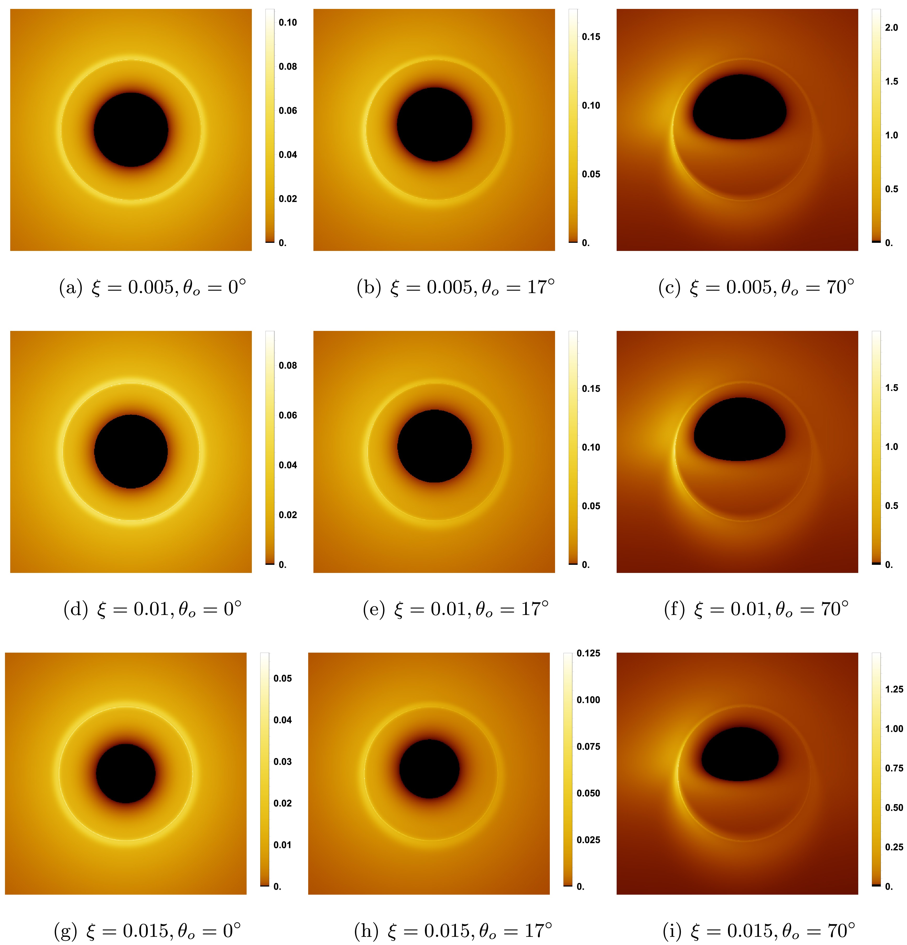
Figure 1. (color online) Shadow images of rotating EGB black holes with a thin accretion disk for
$ M=1 $ and$ a=0.2 $ .When
$ \theta_o = 0^\circ $ (the first column), the inner shadow is perfectly circular, and the photon ring forms a symmetric annulus. This occurs because, at$ \theta_o = 0^\circ $ , the observer's line of sight is perpendicular to the equatorial plane and aligned with the rotation axes of both the accretion disk and the black hole. When$ \theta_o = 17^\circ $ (the second column), the inner shadow becomes slightly deformed, and the photon ring shifts toward the lower right. As$ \theta_o $ increases to$ 70^\circ $ (the third column), the inner shadow is significantly distorted into a ''D''-shaped structure, and a crescent-shaped bright region emerges on the left side of the photon ring, where the brightness is markedly higher than elsewhere. This phenomenon arises because a higher inclination angle amplifies the Doppler effect: in a prograde accretion disk, light rays on the left side move toward the observer, producing a blueshift that enhances the photon energy and brightens the image, whereas light rays on the right side move away, producing a redshift that reduces photon energy and darkens the image.Comparing the rows reveals that as ξ increases, the inner shadow's shape remains unchanged while its size gradually decreases. Notably, regardless of the parameter variations, both the inner shadow and the photon ring persist, indicating that they are intrinsic features of the spacetime described by the metric (7).
To provide a more intuitive illustration of the number of times light rays cross the equatorial plane, Fig. 2 shows the lensing bands of the rotating EGB black hole for two values of the GB coupling constant:
$ \xi = 0.005 $ and$ \xi = 0.015 $ . In Fig. 2, the black, purple, yellow, and red regions represent light rays that cross the equatorial plane zero, one, two, and more than two times, corresponding, respectively, to the inner shadow, the direct image, the lensed image, and the higher-order images. It can be seen that the direct image occupies the widest region, whereas the higher-order images are always contained within the area of the lensed image. When the observation inclination angle is$ \theta_o = 0^\circ $ (the first column), both the lensed and higher-order images exhibit concentric ring structures that share the same center as the inner shadow. As ξ increases, the ring radii slightly decrease. When$ \theta_o $ increases to$ 17^\circ $ (the second column), the lensed and higher-order images shift downward on the screen, and the ring structures become asymmetric. When$ \theta_o $ further increases to$ 70^\circ $ (the third column), the inner shadow, lensed image, and higher-order images are all significantly distorted. In particular, the lensed image extends markedly toward the lower part of the screen, while the higher-order images become more distinguishable in the lower region than in the upper region. The above analysis indicates that the GB coupling constant ξ primarily affects the overall size of the black hole shadow, whereas the observation inclination angle$ \theta_o $ governs the spatial distribution of the inner shadow and the lensed images.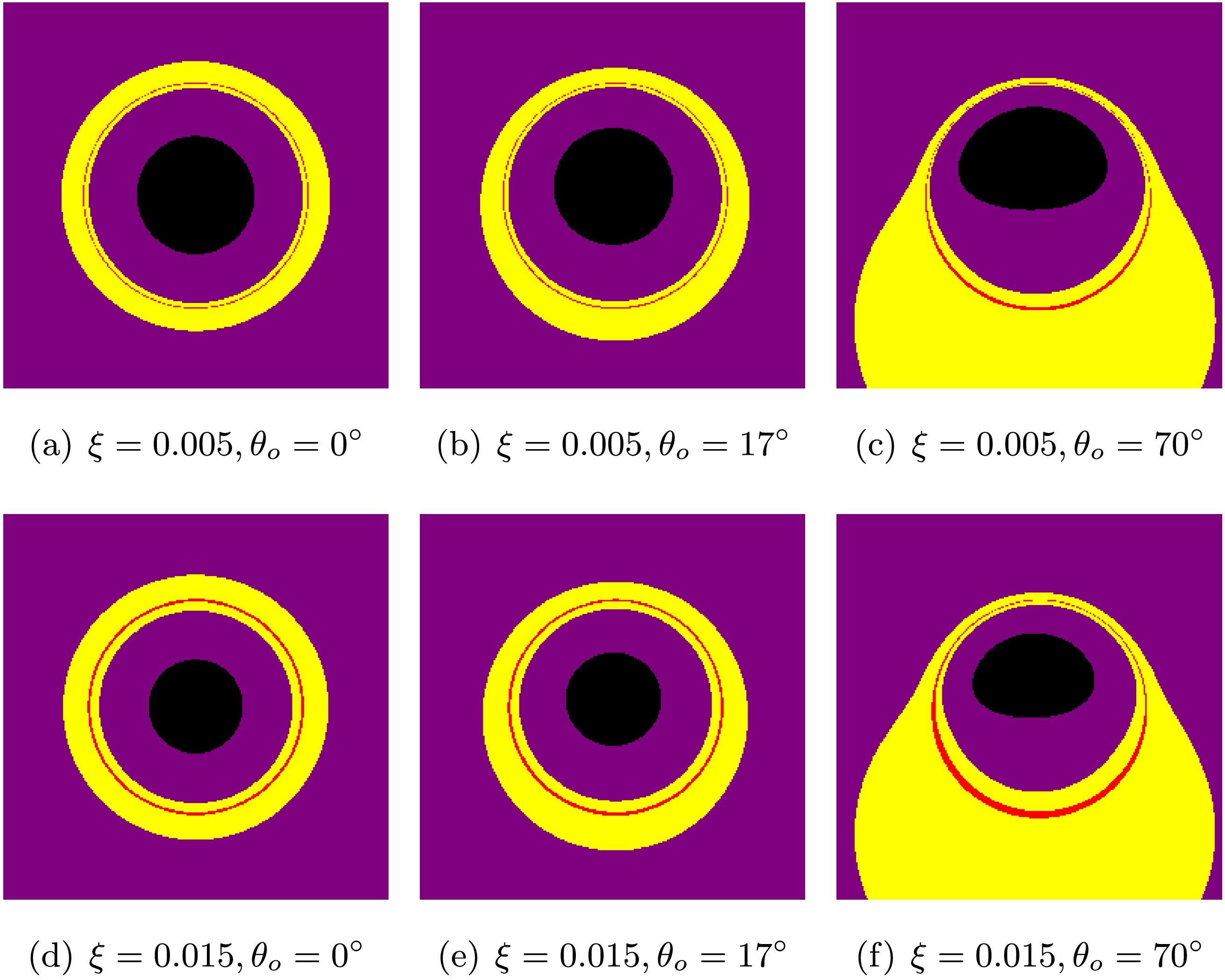
Figure 2. (color online) The lensing bands of rotating EGB black holes with
$ a = 0.2 $ . The black, purple, yellow, and red regions correspond to the inner shadow, direct image, lensed image, and higher-order images, respectively.Figure 3 illustrates the influence of the spin parameter a on the shadow images for fixed
$ \xi=0.005 $ , and Fig. 4 shows the corresponding lensing bands. From Fig. 3, increasing a reduces the sizes of both the inner shadow and the photon ring, while increasing$ \theta_o $ deforms the inner shadow. Comparing each column of images reveals a noteworthy phenomenon: for fixed a and ξ, changing$ \theta_o $ alters the brightness symmetry of the photon ring but leaves its position nearly unchanged. For the spacetime described by the metric (7), the photon ring position is uniquely determined by the photon equations of motion once the spacetime parameters are specified. As shown in Fig. 4, the effect of a on the lensing bands is similar to that of ξ. In the lower-left region of Fig. 4(f), the higher-order image zone is clearly visible because a larger spin parameter and a higher observer inclination enhance the frame-dragging effect and Doppler redshift.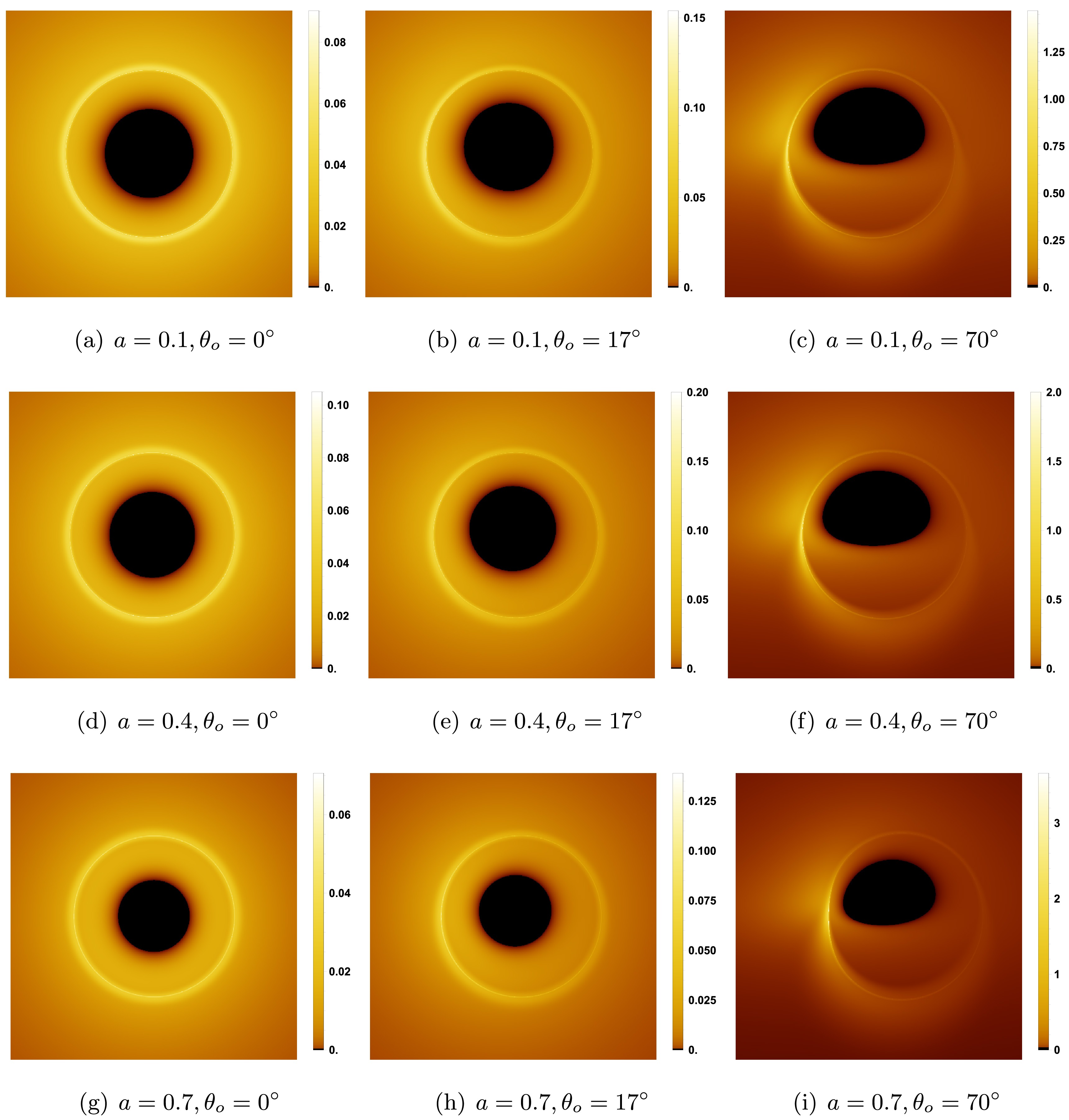
Figure 3. (color online) Shadow images of rotating EGB black holes with a thin accretion disk, for
$ M = 1 $ and$ \xi = 0.005 $ .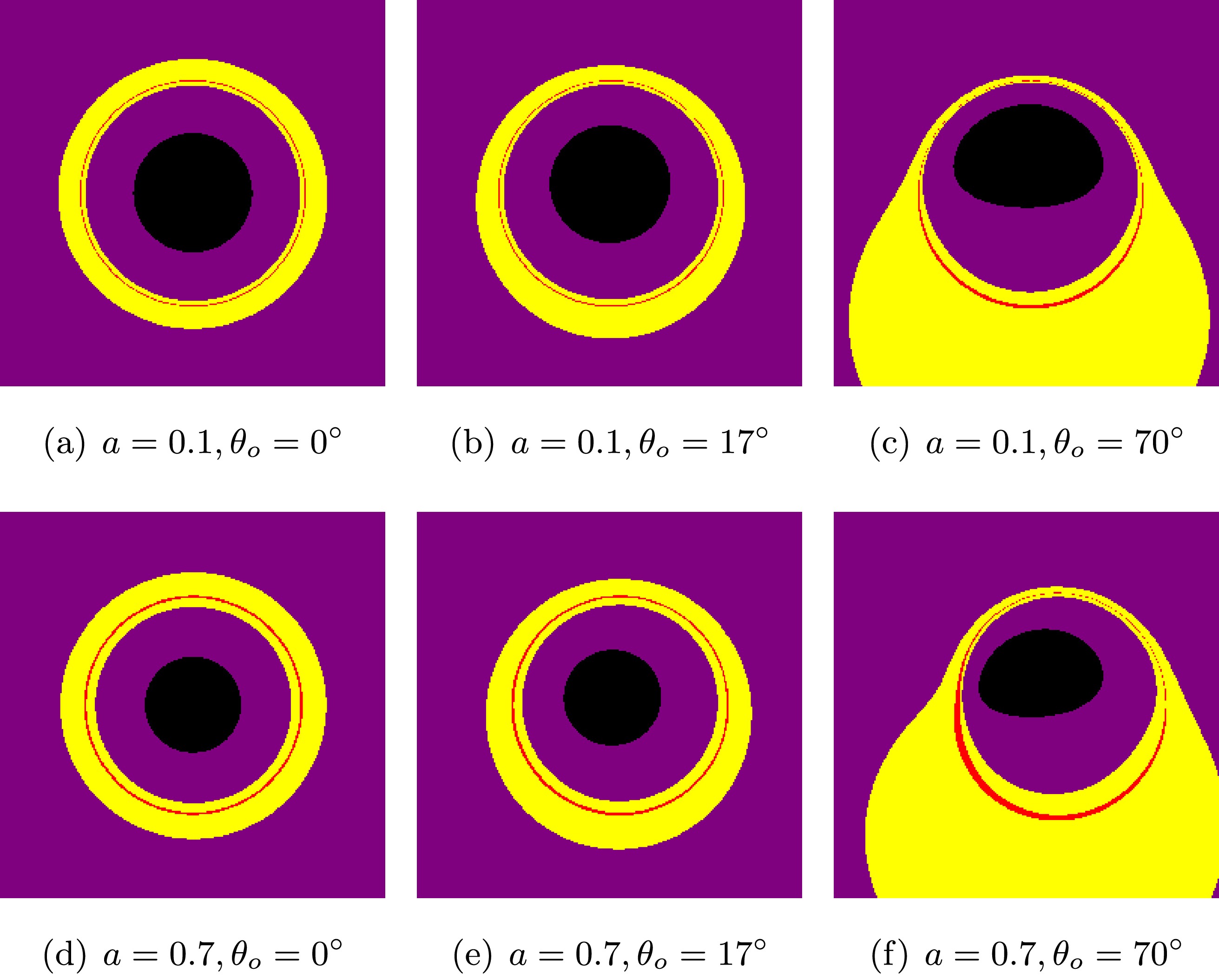
Figure 4. (color online) The lensing bands of rotating EGB black holes with
$ \xi = 0.005 $ : the black, purple, yellow, and red regions correspond to the inner shadow, the direct image, the lensed image, and the higher-order images, respectively.To further analyze the effect of parameter variations on the intensity, Fig. 5 presents the intensity cuts along the X-axis with
$ \theta_o = 0^\circ $ held fixed. The intensity cuts are symmetrically distributed with respect to the Y-axis. Near the origin, the intensity vanishes, corresponding to the event horizon, while the two peaks correspond to the photon ring. As a or ξ increases, the peak values of the intensity cuts gradually decrease, indicating a reduction in the brightness of the photon ring. For a Schwarzschild black hole of unit mass, the photon ring lies at$ r_p = 3 $ ; however, in the black hole models discussed in this work,$ r_p $ is always greater than$ 3 $ , suggesting that the introduction of the GB coupling constant ξ increases the photon ring radius.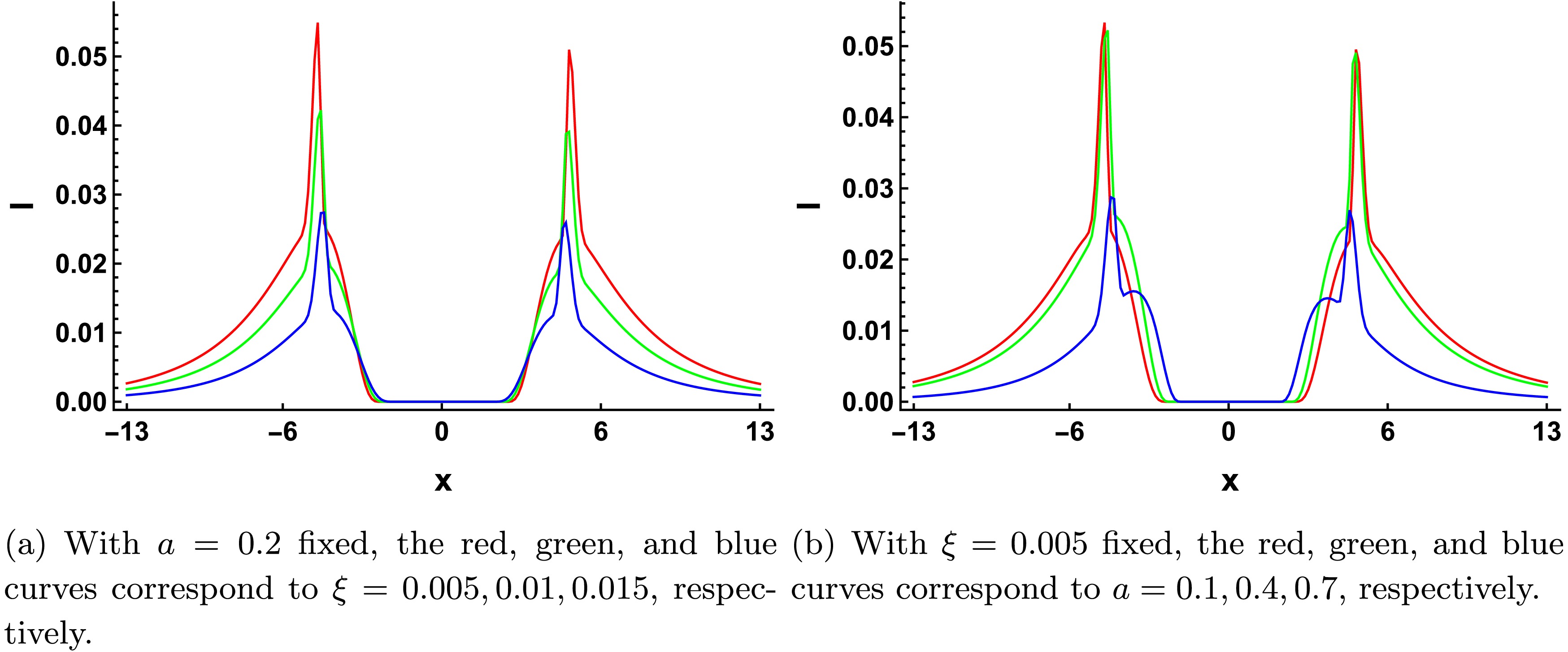
Figure 5. (color online) Intensity cuts along the X-axis for
$ \theta_o = 0^\circ $ . -
This subsection presents the numerical results for the shadow images of a rotating EGB black hole under the thin accretion disk model. For the spacetime described by Eq. (7), we set the black hole mass to
$ M=1 $ and focus on examining the effects of the GB coupling constant ξ, the spin parameter a, and the observer inclination angle$ \theta_o $ on the shadow images. In the numerical calculations, the observer is placed at$ r_o = 500M = 500 $ , and the inclination angles are chosen as$ \theta_o = 0^\circ $ ,$ 17^\circ $ , and$ 70^\circ $ . A prograde accretion disk configuration is adopted, where the disk rotates in the same direction as the black hole spin.The effect of the GB coupling constant ξ on the shadow images is illustrated in Fig. 1, with
$ \xi = 0.005 $ ,$ 0.01 $ , and$ 0.015 $ from top to bottom and the spin parameter fixed at$ a = 0.2 $ . In each image, a distinct dark region appears at the center, known as the inner shadow [73]. Light rays that fall directly into the event horizon (i.e.,$ n = 0 $ ) lead to$ \tilde{I}_{o} = 0 $ according to Eq. (29), meaning that the corresponding pixels in the inner shadow are completely black. Outside the inner shadow lies a luminous ring, referred to as the photon ring, which originates from light rays that cross the equatorial plane multiple times. Each time a photon intersects the accretion disk, its energy increases, thereby enhancing the intensity of the corresponding pixel. Consequently, the photon ring appears significantly brighter than the surrounding region.
Figure 1. (color online) Shadow images of rotating EGB black holes with a thin accretion disk for
$ M=1 $ and$ a=0.2 $ .When
$ \theta_o = 0^\circ $ (the first column), the inner shadow is perfectly circular, and the photon ring forms a symmetric annulus. This occurs because, at$ \theta_o = 0^\circ $ , the observer's line of sight is perpendicular to the equatorial plane and aligned with the rotation axes of both the accretion disk and the black hole. When$ \theta_o = 17^\circ $ (the second column), the inner shadow becomes slightly deformed, and the photon ring shifts toward the lower right. As$ \theta_o $ increases to$ 70^\circ $ (the third column), the inner shadow is significantly distorted into a ''D''-shaped structure, and a crescent-shaped bright region emerges on the left side of the photon ring, where the brightness is markedly higher than elsewhere. This phenomenon arises because a higher inclination angle amplifies the Doppler effect: in a prograde accretion disk, light rays on the left side move toward the observer, producing a blueshift that enhances the photon energy and brightens the image, whereas light rays on the right side move away, producing a redshift that reduces photon energy and darkens the image.Comparing the rows reveals that as ξ increases, the inner shadow's shape remains unchanged while its size gradually decreases. Notably, regardless of the parameter variations, both the inner shadow and the photon ring persist, indicating that they are intrinsic features of the spacetime described by the metric (7).
To provide a more intuitive illustration of the number of times light rays cross the equatorial plane, Fig. 2 shows the lensing bands of the rotating EGB black hole for two values of the GB coupling constant:
$ \xi = 0.005 $ and$ \xi = 0.015 $ . In Fig. 2, the black, purple, yellow, and red regions represent light rays that cross the equatorial plane zero, one, two, and more than two times, corresponding, respectively, to the inner shadow, the direct image, the lensed image, and the higher-order images. It can be seen that the direct image occupies the widest region, whereas the higher-order images are always contained within the area of the lensed image. When the observation inclination angle is$ \theta_o = 0^\circ $ (the first column), both the lensed and higher-order images exhibit concentric ring structures that share the same center as the inner shadow. As ξ increases, the ring radii slightly decrease. When$ \theta_o $ increases to$ 17^\circ $ (the second column), the lensed and higher-order images shift downward on the screen, and the ring structures become asymmetric. When$ \theta_o $ further increases to$ 70^\circ $ (the third column), the inner shadow, lensed image, and higher-order images are all significantly distorted. In particular, the lensed image extends markedly toward the lower part of the screen, while the higher-order images become more distinguishable in the lower region than in the upper region. The above analysis indicates that the GB coupling constant ξ primarily affects the overall size of the black hole shadow, whereas the observation inclination angle$ \theta_o $ governs the spatial distribution of the inner shadow and the lensed images.
Figure 2. (color online) The lensing bands of rotating EGB black holes with
$ a = 0.2 $ . The black, purple, yellow, and red regions correspond to the inner shadow, direct image, lensed image, and higher-order images, respectively.Figure 3 illustrates the influence of the spin parameter a on the shadow images for fixed
$ \xi=0.005 $ , and Fig. 4 shows the corresponding lensing bands. From Fig. 3, increasing a reduces the sizes of both the inner shadow and the photon ring, while increasing$ \theta_o $ deforms the inner shadow. Comparing each column of images reveals a noteworthy phenomenon: for fixed a and ξ, changing$ \theta_o $ alters the brightness symmetry of the photon ring but leaves its position nearly unchanged. For the spacetime described by the metric (7), the photon ring position is uniquely determined by the photon equations of motion once the spacetime parameters are specified. As shown in Fig. 4, the effect of a on the lensing bands is similar to that of ξ. In the lower-left region of Fig. 4(f), the higher-order image zone is clearly visible because a larger spin parameter and a higher observer inclination enhance the frame-dragging effect and Doppler redshift.
Figure 3. (color online) Shadow images of rotating EGB black holes with a thin accretion disk, for
$ M = 1 $ and$ \xi = 0.005 $ .
Figure 4. (color online) The lensing bands of rotating EGB black holes with
$ \xi = 0.005 $ : the black, purple, yellow, and red regions correspond to the inner shadow, the direct image, the lensed image, and the higher-order images, respectively.To further analyze the effect of parameter variations on the intensity, Fig. 5 presents the intensity cuts along the X-axis with
$ \theta_o = 0^\circ $ held fixed. The intensity cuts are symmetrically distributed with respect to the Y-axis. Near the origin, the intensity vanishes, corresponding to the event horizon, while the two peaks correspond to the photon ring. As a or ξ increases, the peak values of the intensity cuts gradually decrease, indicating a reduction in the brightness of the photon ring. For a Schwarzschild black hole of unit mass, the photon ring lies at$ r_p = 3 $ ; however, in the black hole models discussed in this work,$ r_p $ is always greater than$ 3 $ , suggesting that the introduction of the GB coupling constant ξ increases the photon ring radius.
Figure 5. (color online) Intensity cuts along the X-axis for
$ \theta_o = 0^\circ $ . -
This subsection presents the numerical results for the shadow images of a rotating EGB black hole under the thin accretion disk model. For the spacetime described by Eq. (7), we set the black hole mass to
$ M=1 $ and focus on examining the effects of the GB coupling constant ξ, the spin parameter a, and the observer inclination angle$ \theta_o $ on the shadow images. In the numerical calculations, the observer is placed at$ r_o = 500M = 500 $ , and the inclination angles are chosen as$ \theta_o = 0^\circ $ ,$ 17^\circ $ , and$ 70^\circ $ . A prograde accretion disk configuration is adopted, where the disk rotates in the same direction as the black hole spin.The effect of the GB coupling constant ξ on the shadow images is illustrated in Fig. 1, with
$ \xi = 0.005 $ ,$ 0.01 $ , and$ 0.015 $ from top to bottom and the spin parameter fixed at$ a = 0.2 $ . In each image, a distinct dark region appears at the center, known as the inner shadow [73]. Light rays that fall directly into the event horizon (i.e.,$ n = 0 $ ) lead to$ \tilde{I}_{o} = 0 $ according to Eq. (29), meaning that the corresponding pixels in the inner shadow are completely black. Outside the inner shadow lies a luminous ring, referred to as the photon ring, which originates from light rays that cross the equatorial plane multiple times. Each time a photon intersects the accretion disk, its energy increases, thereby enhancing the intensity of the corresponding pixel. Consequently, the photon ring appears significantly brighter than the surrounding region.
Figure 1. (color online) Shadow images of rotating EGB black holes with a thin accretion disk for
$ M=1 $ and$ a=0.2 $ .When
$ \theta_o = 0^\circ $ (the first column), the inner shadow is perfectly circular, and the photon ring forms a symmetric annulus. This occurs because, at$ \theta_o = 0^\circ $ , the observer's line of sight is perpendicular to the equatorial plane and aligned with the rotation axes of both the accretion disk and the black hole. When$ \theta_o = 17^\circ $ (the second column), the inner shadow becomes slightly deformed, and the photon ring shifts toward the lower right. As$ \theta_o $ increases to$ 70^\circ $ (the third column), the inner shadow is significantly distorted into a ''D''-shaped structure, and a crescent-shaped bright region emerges on the left side of the photon ring, where the brightness is markedly higher than elsewhere. This phenomenon arises because a higher inclination angle amplifies the Doppler effect: in a prograde accretion disk, light rays on the left side move toward the observer, producing a blueshift that enhances the photon energy and brightens the image, whereas light rays on the right side move away, producing a redshift that reduces photon energy and darkens the image.Comparing the rows reveals that as ξ increases, the inner shadow's shape remains unchanged while its size gradually decreases. Notably, regardless of the parameter variations, both the inner shadow and the photon ring persist, indicating that they are intrinsic features of the spacetime described by the metric (7).
To provide a more intuitive illustration of the number of times light rays cross the equatorial plane, Fig. 2 shows the lensing bands of the rotating EGB black hole for two values of the GB coupling constant:
$ \xi = 0.005 $ and$ \xi = 0.015 $ . In Fig. 2, the black, purple, yellow, and red regions represent light rays that cross the equatorial plane zero, one, two, and more than two times, corresponding, respectively, to the inner shadow, the direct image, the lensed image, and the higher-order images. It can be seen that the direct image occupies the widest region, whereas the higher-order images are always contained within the area of the lensed image. When the observation inclination angle is$ \theta_o = 0^\circ $ (the first column), both the lensed and higher-order images exhibit concentric ring structures that share the same center as the inner shadow. As ξ increases, the ring radii slightly decrease. When$ \theta_o $ increases to$ 17^\circ $ (the second column), the lensed and higher-order images shift downward on the screen, and the ring structures become asymmetric. When$ \theta_o $ further increases to$ 70^\circ $ (the third column), the inner shadow, lensed image, and higher-order images are all significantly distorted. In particular, the lensed image extends markedly toward the lower part of the screen, while the higher-order images become more distinguishable in the lower region than in the upper region. The above analysis indicates that the GB coupling constant ξ primarily affects the overall size of the black hole shadow, whereas the observation inclination angle$ \theta_o $ governs the spatial distribution of the inner shadow and the lensed images.
Figure 2. (color online) The lensing bands of rotating EGB black holes with
$ a = 0.2 $ . The black, purple, yellow, and red regions correspond to the inner shadow, direct image, lensed image, and higher-order images, respectively.Figure 3 illustrates the influence of the spin parameter a on the shadow images for fixed
$ \xi=0.005 $ , and Fig. 4 shows the corresponding lensing bands. From Fig. 3, increasing a reduces the sizes of both the inner shadow and the photon ring, while increasing$ \theta_o $ deforms the inner shadow. Comparing each column of images reveals a noteworthy phenomenon: for fixed a and ξ, changing$ \theta_o $ alters the brightness symmetry of the photon ring but leaves its position nearly unchanged. For the spacetime described by the metric (7), the photon ring position is uniquely determined by the photon equations of motion once the spacetime parameters are specified. As shown in Fig. 4, the effect of a on the lensing bands is similar to that of ξ. In the lower-left region of Fig. 4(f), the higher-order image zone is clearly visible because a larger spin parameter and a higher observer inclination enhance the frame-dragging effect and Doppler redshift.
Figure 3. (color online) Shadow images of rotating EGB black holes with a thin accretion disk, for
$ M = 1 $ and$ \xi = 0.005 $ .
Figure 4. (color online) The lensing bands of rotating EGB black holes with
$ \xi = 0.005 $ : the black, purple, yellow, and red regions correspond to the inner shadow, the direct image, the lensed image, and the higher-order images, respectively.To further analyze the effect of parameter variations on the intensity, Fig. 5 presents the intensity cuts along the X-axis with
$ \theta_o = 0^\circ $ held fixed. The intensity cuts are symmetrically distributed with respect to the Y-axis. Near the origin, the intensity vanishes, corresponding to the event horizon, while the two peaks correspond to the photon ring. As a or ξ increases, the peak values of the intensity cuts gradually decrease, indicating a reduction in the brightness of the photon ring. For a Schwarzschild black hole of unit mass, the photon ring lies at$ r_p = 3 $ ; however, in the black hole models discussed in this work,$ r_p $ is always greater than$ 3 $ , suggesting that the introduction of the GB coupling constant ξ increases the photon ring radius.
Figure 5. (color online) Intensity cuts along the X-axis for
$ \theta_o = 0^\circ $ . -
This subsection presents the numerical results for the shadow images of a rotating EGB black hole under the thin accretion disk model. For the spacetime described by Eq. (7), we set the black hole mass to
$ M=1 $ and focus on examining the effects of the GB coupling constant ξ, the spin parameter a, and the observer inclination angle$ \theta_o $ on the shadow images. In the numerical calculations, the observer is placed at$ r_o = 500M = 500 $ , and the inclination angles are chosen as$ \theta_o = 0^\circ $ ,$ 17^\circ $ , and$ 70^\circ $ . A prograde accretion disk configuration is adopted, where the disk rotates in the same direction as the black hole spin.The effect of the GB coupling constant ξ on the shadow images is illustrated in Fig. 1, with
$ \xi = 0.005 $ ,$ 0.01 $ , and$ 0.015 $ from top to bottom and the spin parameter fixed at$ a = 0.2 $ . In each image, a distinct dark region appears at the center, known as the inner shadow [73]. Light rays that fall directly into the event horizon (i.e.,$ n = 0 $ ) lead to$ \tilde{I}_{o} = 0 $ according to Eq. (29), meaning that the corresponding pixels in the inner shadow are completely black. Outside the inner shadow lies a luminous ring, referred to as the photon ring, which originates from light rays that cross the equatorial plane multiple times. Each time a photon intersects the accretion disk, its energy increases, thereby enhancing the intensity of the corresponding pixel. Consequently, the photon ring appears significantly brighter than the surrounding region.
Figure 1. (color online) Shadow images of rotating EGB black holes with a thin accretion disk for
$ M=1 $ and$ a=0.2 $ .When
$ \theta_o = 0^\circ $ (the first column), the inner shadow is perfectly circular, and the photon ring forms a symmetric annulus. This occurs because, at$ \theta_o = 0^\circ $ , the observer's line of sight is perpendicular to the equatorial plane and aligned with the rotation axes of both the accretion disk and the black hole. When$ \theta_o = 17^\circ $ (the second column), the inner shadow becomes slightly deformed, and the photon ring shifts toward the lower right. As$ \theta_o $ increases to$ 70^\circ $ (the third column), the inner shadow is significantly distorted into a ''D''-shaped structure, and a crescent-shaped bright region emerges on the left side of the photon ring, where the brightness is markedly higher than elsewhere. This phenomenon arises because a higher inclination angle amplifies the Doppler effect: in a prograde accretion disk, light rays on the left side move toward the observer, producing a blueshift that enhances the photon energy and brightens the image, whereas light rays on the right side move away, producing a redshift that reduces photon energy and darkens the image.Comparing the rows reveals that as ξ increases, the inner shadow's shape remains unchanged while its size gradually decreases. Notably, regardless of the parameter variations, both the inner shadow and the photon ring persist, indicating that they are intrinsic features of the spacetime described by the metric (7).
To provide a more intuitive illustration of the number of times light rays cross the equatorial plane, Fig. 2 shows the lensing bands of the rotating EGB black hole for two values of the GB coupling constant:
$ \xi = 0.005 $ and$ \xi = 0.015 $ . In Fig. 2, the black, purple, yellow, and red regions represent light rays that cross the equatorial plane zero, one, two, and more than two times, corresponding, respectively, to the inner shadow, the direct image, the lensed image, and the higher-order images. It can be seen that the direct image occupies the widest region, whereas the higher-order images are always contained within the area of the lensed image. When the observation inclination angle is$ \theta_o = 0^\circ $ (the first column), both the lensed and higher-order images exhibit concentric ring structures that share the same center as the inner shadow. As ξ increases, the ring radii slightly decrease. When$ \theta_o $ increases to$ 17^\circ $ (the second column), the lensed and higher-order images shift downward on the screen, and the ring structures become asymmetric. When$ \theta_o $ further increases to$ 70^\circ $ (the third column), the inner shadow, lensed image, and higher-order images are all significantly distorted. In particular, the lensed image extends markedly toward the lower part of the screen, while the higher-order images become more distinguishable in the lower region than in the upper region. The above analysis indicates that the GB coupling constant ξ primarily affects the overall size of the black hole shadow, whereas the observation inclination angle$ \theta_o $ governs the spatial distribution of the inner shadow and the lensed images.
Figure 2. (color online) The lensing bands of rotating EGB black holes with
$ a = 0.2 $ . The black, purple, yellow, and red regions correspond to the inner shadow, direct image, lensed image, and higher-order images, respectively.Figure 3 illustrates the influence of the spin parameter a on the shadow images for fixed
$ \xi=0.005 $ , and Fig. 4 shows the corresponding lensing bands. From Fig. 3, increasing a reduces the sizes of both the inner shadow and the photon ring, while increasing$ \theta_o $ deforms the inner shadow. Comparing each column of images reveals a noteworthy phenomenon: for fixed a and ξ, changing$ \theta_o $ alters the brightness symmetry of the photon ring but leaves its position nearly unchanged. For the spacetime described by the metric (7), the photon ring position is uniquely determined by the photon equations of motion once the spacetime parameters are specified. As shown in Fig. 4, the effect of a on the lensing bands is similar to that of ξ. In the lower-left region of Fig. 4(f), the higher-order image zone is clearly visible because a larger spin parameter and a higher observer inclination enhance the frame-dragging effect and Doppler redshift.
Figure 3. (color online) Shadow images of rotating EGB black holes with a thin accretion disk, for
$ M = 1 $ and$ \xi = 0.005 $ .
Figure 4. (color online) The lensing bands of rotating EGB black holes with
$ \xi = 0.005 $ : the black, purple, yellow, and red regions correspond to the inner shadow, the direct image, the lensed image, and the higher-order images, respectively.To further analyze the effect of parameter variations on the intensity, Fig. 5 presents the intensity cuts along the X-axis with
$ \theta_o = 0^\circ $ held fixed. The intensity cuts are symmetrically distributed with respect to the Y-axis. Near the origin, the intensity vanishes, corresponding to the event horizon, while the two peaks correspond to the photon ring. As a or ξ increases, the peak values of the intensity cuts gradually decrease, indicating a reduction in the brightness of the photon ring. For a Schwarzschild black hole of unit mass, the photon ring lies at$ r_p = 3 $ ; however, in the black hole models discussed in this work,$ r_p $ is always greater than$ 3 $ , suggesting that the introduction of the GB coupling constant ξ increases the photon ring radius.
Figure 5. (color online) Intensity cuts along the X-axis for
$ \theta_o = 0^\circ $ . -
This subsection presents the numerical results for the shadow images of a rotating EGB black hole under the thin accretion disk model. For the spacetime described by Eq. (7), we set the black hole mass to
$ M=1 $ and focus on examining the effects of the GB coupling constant ξ, the spin parameter a, and the observer inclination angle$ \theta_o $ on the shadow images. In the numerical calculations, the observer is placed at$ r_o = 500M = 500 $ , and the inclination angles are chosen as$ \theta_o = 0^\circ $ ,$ 17^\circ $ , and$ 70^\circ $ . A prograde accretion disk configuration is adopted, where the disk rotates in the same direction as the black hole spin.The effect of the GB coupling constant ξ on the shadow images is illustrated in Fig. 1, with
$ \xi = 0.005 $ ,$ 0.01 $ , and$ 0.015 $ from top to bottom and the spin parameter fixed at$ a = 0.2 $ . In each image, a distinct dark region appears at the center, known as the inner shadow [73]. Light rays that fall directly into the event horizon (i.e.,$ n = 0 $ ) lead to$ \tilde{I}_{o} = 0 $ according to Eq. (29), meaning that the corresponding pixels in the inner shadow are completely black. Outside the inner shadow lies a luminous ring, referred to as the photon ring, which originates from light rays that cross the equatorial plane multiple times. Each time a photon intersects the accretion disk, its energy increases, thereby enhancing the intensity of the corresponding pixel. Consequently, the photon ring appears significantly brighter than the surrounding region.
Figure 1. (color online) Shadow images of rotating EGB black holes with a thin accretion disk for
$ M=1 $ and$ a=0.2 $ .When
$ \theta_o = 0^\circ $ (the first column), the inner shadow is perfectly circular, and the photon ring forms a symmetric annulus. This occurs because, at$ \theta_o = 0^\circ $ , the observer's line of sight is perpendicular to the equatorial plane and aligned with the rotation axes of both the accretion disk and the black hole. When$ \theta_o = 17^\circ $ (the second column), the inner shadow becomes slightly deformed, and the photon ring shifts toward the lower right. As$ \theta_o $ increases to$ 70^\circ $ (the third column), the inner shadow is significantly distorted into a ''D''-shaped structure, and a crescent-shaped bright region emerges on the left side of the photon ring, where the brightness is markedly higher than elsewhere. This phenomenon arises because a higher inclination angle amplifies the Doppler effect: in a prograde accretion disk, light rays on the left side move toward the observer, producing a blueshift that enhances the photon energy and brightens the image, whereas light rays on the right side move away, producing a redshift that reduces photon energy and darkens the image.Comparing the rows reveals that as ξ increases, the inner shadow's shape remains unchanged while its size gradually decreases. Notably, regardless of the parameter variations, both the inner shadow and the photon ring persist, indicating that they are intrinsic features of the spacetime described by the metric (7).
To provide a more intuitive illustration of the number of times light rays cross the equatorial plane, Fig. 2 shows the lensing bands of the rotating EGB black hole for two values of the GB coupling constant:
$ \xi = 0.005 $ and$ \xi = 0.015 $ . In Fig. 2, the black, purple, yellow, and red regions represent light rays that cross the equatorial plane zero, one, two, and more than two times, corresponding, respectively, to the inner shadow, the direct image, the lensed image, and the higher-order images. It can be seen that the direct image occupies the widest region, whereas the higher-order images are always contained within the area of the lensed image. When the observation inclination angle is$ \theta_o = 0^\circ $ (the first column), both the lensed and higher-order images exhibit concentric ring structures that share the same center as the inner shadow. As ξ increases, the ring radii slightly decrease. When$ \theta_o $ increases to$ 17^\circ $ (the second column), the lensed and higher-order images shift downward on the screen, and the ring structures become asymmetric. When$ \theta_o $ further increases to$ 70^\circ $ (the third column), the inner shadow, lensed image, and higher-order images are all significantly distorted. In particular, the lensed image extends markedly toward the lower part of the screen, while the higher-order images become more distinguishable in the lower region than in the upper region. The above analysis indicates that the GB coupling constant ξ primarily affects the overall size of the black hole shadow, whereas the observation inclination angle$ \theta_o $ governs the spatial distribution of the inner shadow and the lensed images.
Figure 2. (color online) The lensing bands of rotating EGB black holes with
$ a = 0.2 $ . The black, purple, yellow, and red regions correspond to the inner shadow, direct image, lensed image, and higher-order images, respectively.Figure 3 illustrates the influence of the spin parameter a on the shadow images for fixed
$ \xi=0.005 $ , and Fig. 4 shows the corresponding lensing bands. From Fig. 3, increasing a reduces the sizes of both the inner shadow and the photon ring, while increasing$ \theta_o $ deforms the inner shadow. Comparing each column of images reveals a noteworthy phenomenon: for fixed a and ξ, changing$ \theta_o $ alters the brightness symmetry of the photon ring but leaves its position nearly unchanged. For the spacetime described by the metric (7), the photon ring position is uniquely determined by the photon equations of motion once the spacetime parameters are specified. As shown in Fig. 4, the effect of a on the lensing bands is similar to that of ξ. In the lower-left region of Fig. 4(f), the higher-order image zone is clearly visible because a larger spin parameter and a higher observer inclination enhance the frame-dragging effect and Doppler redshift.
Figure 3. (color online) Shadow images of rotating EGB black holes with a thin accretion disk, for
$ M = 1 $ and$ \xi = 0.005 $ .
Figure 4. (color online) The lensing bands of rotating EGB black holes with
$ \xi = 0.005 $ : the black, purple, yellow, and red regions correspond to the inner shadow, the direct image, the lensed image, and the higher-order images, respectively.To further analyze the effect of parameter variations on the intensity, Fig. 5 presents the intensity cuts along the X-axis with
$ \theta_o = 0^\circ $ held fixed. The intensity cuts are symmetrically distributed with respect to the Y-axis. Near the origin, the intensity vanishes, corresponding to the event horizon, while the two peaks correspond to the photon ring. As a or ξ increases, the peak values of the intensity cuts gradually decrease, indicating a reduction in the brightness of the photon ring. For a Schwarzschild black hole of unit mass, the photon ring lies at$ r_p = 3 $ ; however, in the black hole models discussed in this work,$ r_p $ is always greater than$ 3 $ , suggesting that the introduction of the GB coupling constant ξ increases the photon ring radius.
Figure 5. (color online) Intensity cuts along the X-axis for
$ \theta_o = 0^\circ $ . -
To gain a more comprehensive understanding of the features of the rotating EGB spacetime, this section investigates its polarization images within the thin accretion disk model. We assume that the source of polarized radiation is synchrotron emission produced by electrons in the plasma. For an observer comoving with the plasma, with four-velocity
$ u^\mu $ , in an optically thin medium the polarization direction$ \vec{f} $ of the emitted light is always orthogonal to both the local magnetic field$ \vec{b} $ and the photon wave vector$ \vec{k} $ [34, 74]$ \begin{aligned}[b] \vec{f}=\frac{\vec{k}\times\vec{b}}{|\vec{k}||\vec{b}|}. \end{aligned} $
(34) Equivalently, this condition can be written in a generally covariant form as
$ f^\mu \propto \epsilon^{\mu\nu\alpha\beta}u_\nu k_\alpha b_\beta $ [29, 75]. Additionally, the orthonormality condition$ f^{\mu}f_{\mu}=1 $ must be satisfied. The intensities of linearly polarized light and unpolarized light at the emission point are denoted by the emissivity functions$ \tilde{E}_p $ and$ \tilde{E}_i $ , respectively. For simplicity, we assume that the emission intensity is independent of photon frequency and the magnetic field, depending only on position, i.e.,$ \tilde{E}_i=\tilde{E}_i(r),\tilde{E}_p=q \tilde{E}_i(r), $ where$ q\in[0,1] $ describes the fraction of linearly polarized light in the total emission. If the emitted light is completely linearly polarized,$ q=1 $ . Under the geometric optics approximation, the polarization vector$ f^\mu $ is parallel transported along the photon geodesic$ k^{\nu}\nabla_{\nu}f^{\mu}=0 $ , which can also be expressed as$\dfrac{\rm d}{{\rm d}\tau}f^{\mu}+\Gamma^{\mu}{}_{\nu\alpha}k^{\nu}f^{\alpha}=0,$ where τ is the affine parameter. At the observer’s position, the specific intensity of linearly polarized light$ \tilde{P}_{\nu_o} $ and the total intensity$ \tilde{I}_{\nu_o} $ are given by the same form as in the unpolarized case$ \begin{aligned}[b] \tilde{P}_{\nu_o}= g^3\tilde{E}_p,\qquad \tilde{I}_{\nu_o}=g^3\tilde{E}_i, \end{aligned} $
(35) where g is the redshift factor. In Eq. (18), we construct an orthonormal tetrad for a zero angular momentum observer (ZAMO) at the observer's position and define the imaging screen accordingly. Choosing an orthonormal basis
$ (e_{(\theta)},\,e_{(\varphi)}) $ on the screen, the projection of the polarization vector onto the image plane is given by$ \begin{aligned}[b] f^{(\alpha)}=f^\mu\cdot e_\alpha=-f^\mu\cdot e_\varphi,\qquad f^{(\beta)}=f^\mu\cdot e_\beta=-f^\mu\cdot e_\theta. \end{aligned} $
(36) After determining the polarization vector direction, the total linearly polarized intensity can be obtained by summing the contributions from each emission point in the equatorial plane. The Stokes parameters Q and U satisfy the principle of linear superposition [76]. Therefore, the final results are obtained by summing Q and U [35]
$ \begin{aligned}[b] Q_{\rm all}&=\sum_{n=1}^{N}\chi_n^3\tilde{E}_{pn}\left[\left(f_n^{(\alpha)}\right)^2-\left(f_n^{(\beta)}\right)^2\right],\\ U_{\rm all}&=\sum_{n=1}^{N}\chi_n^3\tilde{E}_{pn}\left(2f_n^{(\alpha)}f_n^{(\beta)}\right). \end{aligned} $
(37) Based on the preceding analysis, the total linearly polarized intensity and the electric vector position angle (EVPA) of the observed light are given by
$ \begin{aligned}[b] \tilde{P}_o=\left(Q_{\rm all}^2+U_{\rm all}^2\right)^{\frac12},\quad\Theta_E=\frac{1}{2}\arctan\frac{U_{\rm all}}{Q_{\rm all}}. \end{aligned} $
(38) After the EVPA is obtained and combined with the polarization intensity, the polarization image of a rotating EGB black hole in a thin accretion disk background can be constructed.
-
To gain a more comprehensive understanding of the features of the rotating EGB spacetime, this section investigates its polarization images within the thin accretion disk model. We assume that the source of polarized radiation is synchrotron emission produced by electrons in the plasma. For an observer comoving with the plasma, with four-velocity
$ u^\mu $ , in an optically thin medium the polarization direction$ \vec{f} $ of the emitted light is always orthogonal to both the local magnetic field$ \vec{b} $ and the photon wave vector$ \vec{k} $ [34, 74]$ \begin{aligned}[b] \vec{f}=\frac{\vec{k}\times\vec{b}}{|\vec{k}||\vec{b}|}. \end{aligned} $
(34) Equivalently, this condition can be written in a generally covariant form as
$ f^\mu \propto \epsilon^{\mu\nu\alpha\beta}u_\nu k_\alpha b_\beta $ [29, 75]. Additionally, the orthonormality condition$ f^{\mu}f_{\mu}=1 $ must be satisfied. The intensities of linearly polarized light and unpolarized light at the emission point are denoted by the emissivity functions$ \tilde{E}_p $ and$ \tilde{E}_i $ , respectively. For simplicity, we assume that the emission intensity is independent of photon frequency and the magnetic field, depending only on position, i.e.,$ \tilde{E}_i=\tilde{E}_i(r),\tilde{E}_p=q \tilde{E}_i(r), $ where$ q\in[0,1] $ describes the fraction of linearly polarized light in the total emission. If the emitted light is completely linearly polarized,$ q=1 $ . Under the geometric optics approximation, the polarization vector$ f^\mu $ is parallel transported along the photon geodesic$ k^{\nu}\nabla_{\nu}f^{\mu}=0 $ , which can also be expressed as$\dfrac{\rm d}{{\rm d}\tau}f^{\mu}+\Gamma^{\mu}{}_{\nu\alpha}k^{\nu}f^{\alpha}=0,$ where τ is the affine parameter. At the observer’s position, the specific intensity of linearly polarized light$ \tilde{P}_{\nu_o} $ and the total intensity$ \tilde{I}_{\nu_o} $ are given by the same form as in the unpolarized case$ \begin{aligned}[b] \tilde{P}_{\nu_o}= g^3\tilde{E}_p,\qquad \tilde{I}_{\nu_o}=g^3\tilde{E}_i, \end{aligned} $
(35) where g is the redshift factor. In Eq. (18), we construct an orthonormal tetrad for a zero angular momentum observer (ZAMO) at the observer's position and define the imaging screen accordingly. Choosing an orthonormal basis
$ (e_{(\theta)},\,e_{(\varphi)}) $ on the screen, the projection of the polarization vector onto the image plane is given by$ \begin{aligned}[b] f^{(\alpha)}=f^\mu\cdot e_\alpha=-f^\mu\cdot e_\varphi,\qquad f^{(\beta)}=f^\mu\cdot e_\beta=-f^\mu\cdot e_\theta. \end{aligned} $
(36) After determining the polarization vector direction, the total linearly polarized intensity can be obtained by summing the contributions from each emission point in the equatorial plane. The Stokes parameters Q and U satisfy the principle of linear superposition [76]. Therefore, the final results are obtained by summing Q and U [35]
$ \begin{aligned}[b] Q_{\rm all}&=\sum_{n=1}^{N}\chi_n^3\tilde{E}_{pn}\left[\left(f_n^{(\alpha)}\right)^2-\left(f_n^{(\beta)}\right)^2\right],\\ U_{\rm all}&=\sum_{n=1}^{N}\chi_n^3\tilde{E}_{pn}\left(2f_n^{(\alpha)}f_n^{(\beta)}\right). \end{aligned} $
(37) Based on the preceding analysis, the total linearly polarized intensity and the electric vector position angle (EVPA) of the observed light are given by
$ \begin{aligned}[b] \tilde{P}_o=\left(Q_{\rm all}^2+U_{\rm all}^2\right)^{\frac12},\quad\Theta_E=\frac{1}{2}\arctan\frac{U_{\rm all}}{Q_{\rm all}}. \end{aligned} $
(38) After the EVPA is obtained and combined with the polarization intensity, the polarization image of a rotating EGB black hole in a thin accretion disk background can be constructed.
-
To gain a more comprehensive understanding of the features of the rotating EGB spacetime, this section investigates its polarization images within the thin accretion disk model. We assume that the source of polarized radiation is synchrotron emission produced by electrons in the plasma. For an observer comoving with the plasma, with four-velocity
$ u^\mu $ , in an optically thin medium the polarization direction$ \vec{f} $ of the emitted light is always orthogonal to both the local magnetic field$ \vec{b} $ and the photon wave vector$ \vec{k} $ [34, 74]$ \begin{aligned}[b] \vec{f}=\frac{\vec{k}\times\vec{b}}{|\vec{k}||\vec{b}|}. \end{aligned} $
(34) Equivalently, this condition can be written in a generally covariant form as
$ f^\mu \propto \epsilon^{\mu\nu\alpha\beta}u_\nu k_\alpha b_\beta $ [29, 75]. Additionally, the orthonormality condition$ f^{\mu}f_{\mu}=1 $ must be satisfied. The intensities of linearly polarized light and unpolarized light at the emission point are denoted by the emissivity functions$ \tilde{E}_p $ and$ \tilde{E}_i $ , respectively. For simplicity, we assume that the emission intensity is independent of photon frequency and the magnetic field, depending only on position, i.e.,$ \tilde{E}_i=\tilde{E}_i(r),\tilde{E}_p=q \tilde{E}_i(r), $ where$ q\in[0,1] $ describes the fraction of linearly polarized light in the total emission. If the emitted light is completely linearly polarized,$ q=1 $ . Under the geometric optics approximation, the polarization vector$ f^\mu $ is parallel transported along the photon geodesic$ k^{\nu}\nabla_{\nu}f^{\mu}=0 $ , which can also be expressed as$\dfrac{\rm d}{{\rm d}\tau}f^{\mu}+\Gamma^{\mu}{}_{\nu\alpha}k^{\nu}f^{\alpha}=0,$ where τ is the affine parameter. At the observer’s position, the specific intensity of linearly polarized light$ \tilde{P}_{\nu_o} $ and the total intensity$ \tilde{I}_{\nu_o} $ are given by the same form as in the unpolarized case$ \begin{aligned}[b] \tilde{P}_{\nu_o}= g^3\tilde{E}_p,\qquad \tilde{I}_{\nu_o}=g^3\tilde{E}_i, \end{aligned} $
(35) where g is the redshift factor. In Eq. (18), we construct an orthonormal tetrad for a zero angular momentum observer (ZAMO) at the observer's position and define the imaging screen accordingly. Choosing an orthonormal basis
$ (e_{(\theta)},\,e_{(\varphi)}) $ on the screen, the projection of the polarization vector onto the image plane is given by$ \begin{aligned}[b] f^{(\alpha)}=f^\mu\cdot e_\alpha=-f^\mu\cdot e_\varphi,\qquad f^{(\beta)}=f^\mu\cdot e_\beta=-f^\mu\cdot e_\theta. \end{aligned} $
(36) After determining the polarization vector direction, the total linearly polarized intensity can be obtained by summing the contributions from each emission point in the equatorial plane. The Stokes parameters Q and U satisfy the principle of linear superposition [76]. Therefore, the final results are obtained by summing Q and U [35]
$ \begin{aligned}[b] Q_{\rm all}&=\sum_{n=1}^{N}\chi_n^3\tilde{E}_{pn}\left[\left(f_n^{(\alpha)}\right)^2-\left(f_n^{(\beta)}\right)^2\right],\\ U_{\rm all}&=\sum_{n=1}^{N}\chi_n^3\tilde{E}_{pn}\left(2f_n^{(\alpha)}f_n^{(\beta)}\right). \end{aligned} $
(37) Based on the preceding analysis, the total linearly polarized intensity and the electric vector position angle (EVPA) of the observed light are given by
$ \begin{aligned}[b] \tilde{P}_o=\left(Q_{\rm all}^2+U_{\rm all}^2\right)^{\frac12},\quad\Theta_E=\frac{1}{2}\arctan\frac{U_{\rm all}}{Q_{\rm all}}. \end{aligned} $
(38) After the EVPA is obtained and combined with the polarization intensity, the polarization image of a rotating EGB black hole in a thin accretion disk background can be constructed.
-
To gain a more comprehensive understanding of the features of the rotating EGB spacetime, this section investigates its polarization images within the thin accretion disk model. We assume that the source of polarized radiation is synchrotron emission produced by electrons in the plasma. For an observer comoving with the plasma, with four-velocity
$ u^\mu $ , in an optically thin medium the polarization direction$ \vec{f} $ of the emitted light is always orthogonal to both the local magnetic field$ \vec{b} $ and the photon wave vector$ \vec{k} $ [34, 74]$ \begin{aligned}[b] \vec{f}=\frac{\vec{k}\times\vec{b}}{|\vec{k}||\vec{b}|}. \end{aligned} $
(34) Equivalently, this condition can be written in a generally covariant form as
$ f^\mu \propto \epsilon^{\mu\nu\alpha\beta}u_\nu k_\alpha b_\beta $ [29, 75]. Additionally, the orthonormality condition$ f^{\mu}f_{\mu}=1 $ must be satisfied. The intensities of linearly polarized light and unpolarized light at the emission point are denoted by the emissivity functions$ \tilde{E}_p $ and$ \tilde{E}_i $ , respectively. For simplicity, we assume that the emission intensity is independent of photon frequency and the magnetic field, depending only on position, i.e.,$ \tilde{E}_i=\tilde{E}_i(r),\tilde{E}_p=q \tilde{E}_i(r), $ where$ q\in[0,1] $ describes the fraction of linearly polarized light in the total emission. If the emitted light is completely linearly polarized,$ q=1 $ . Under the geometric optics approximation, the polarization vector$ f^\mu $ is parallel transported along the photon geodesic$ k^{\nu}\nabla_{\nu}f^{\mu}=0 $ , which can also be expressed as$\dfrac{\rm d}{{\rm d}\tau}f^{\mu}+\Gamma^{\mu}{}_{\nu\alpha}k^{\nu}f^{\alpha}=0,$ where τ is the affine parameter. At the observer’s position, the specific intensity of linearly polarized light$ \tilde{P}_{\nu_o} $ and the total intensity$ \tilde{I}_{\nu_o} $ are given by the same form as in the unpolarized case$ \begin{aligned}[b] \tilde{P}_{\nu_o}= g^3\tilde{E}_p,\qquad \tilde{I}_{\nu_o}=g^3\tilde{E}_i, \end{aligned} $
(35) where g is the redshift factor. In Eq. (18), we construct an orthonormal tetrad for a zero angular momentum observer (ZAMO) at the observer's position and define the imaging screen accordingly. Choosing an orthonormal basis
$ (e_{(\theta)},\,e_{(\varphi)}) $ on the screen, the projection of the polarization vector onto the image plane is given by$ \begin{aligned}[b] f^{(\alpha)}=f^\mu\cdot e_\alpha=-f^\mu\cdot e_\varphi,\qquad f^{(\beta)}=f^\mu\cdot e_\beta=-f^\mu\cdot e_\theta. \end{aligned} $
(36) After determining the polarization vector direction, the total linearly polarized intensity can be obtained by summing the contributions from each emission point in the equatorial plane. The Stokes parameters Q and U satisfy the principle of linear superposition [76]. Therefore, the final results are obtained by summing Q and U [35]
$ \begin{aligned}[b] Q_{\rm all}&=\sum_{n=1}^{N}\chi_n^3\tilde{E}_{pn}\left[\left(f_n^{(\alpha)}\right)^2-\left(f_n^{(\beta)}\right)^2\right],\\ U_{\rm all}&=\sum_{n=1}^{N}\chi_n^3\tilde{E}_{pn}\left(2f_n^{(\alpha)}f_n^{(\beta)}\right). \end{aligned} $
(37) Based on the preceding analysis, the total linearly polarized intensity and the electric vector position angle (EVPA) of the observed light are given by
$ \begin{aligned}[b] \tilde{P}_o=\left(Q_{\rm all}^2+U_{\rm all}^2\right)^{\frac12},\quad\Theta_E=\frac{1}{2}\arctan\frac{U_{\rm all}}{Q_{\rm all}}. \end{aligned} $
(38) After the EVPA is obtained and combined with the polarization intensity, the polarization image of a rotating EGB black hole in a thin accretion disk background can be constructed.
-
To gain a more comprehensive understanding of the features of the rotating EGB spacetime, this section investigates its polarization images within the thin accretion disk model. We assume that the source of polarized radiation is synchrotron emission produced by electrons in the plasma. For an observer comoving with the plasma, with four-velocity
$ u^\mu $ , in an optically thin medium the polarization direction$ \vec{f} $ of the emitted light is always orthogonal to both the local magnetic field$ \vec{b} $ and the photon wave vector$ \vec{k} $ [34, 74]$ \begin{aligned}[b] \vec{f}=\frac{\vec{k}\times\vec{b}}{|\vec{k}||\vec{b}|}. \end{aligned} $
(34) Equivalently, this condition can be written in a generally covariant form as
$ f^\mu \propto \epsilon^{\mu\nu\alpha\beta}u_\nu k_\alpha b_\beta $ [29, 75]. Additionally, the orthonormality condition$ f^{\mu}f_{\mu}=1 $ must be satisfied. The intensities of linearly polarized light and unpolarized light at the emission point are denoted by the emissivity functions$ \tilde{E}_p $ and$ \tilde{E}_i $ , respectively. For simplicity, we assume that the emission intensity is independent of photon frequency and the magnetic field, depending only on position, i.e.,$ \tilde{E}_i=\tilde{E}_i(r),\tilde{E}_p=q \tilde{E}_i(r), $ where$ q\in[0,1] $ describes the fraction of linearly polarized light in the total emission. If the emitted light is completely linearly polarized,$ q=1 $ . Under the geometric optics approximation, the polarization vector$ f^\mu $ is parallel transported along the photon geodesic$ k^{\nu}\nabla_{\nu}f^{\mu}=0 $ , which can also be expressed as$\dfrac{\rm d}{{\rm d}\tau}f^{\mu}+\Gamma^{\mu}{}_{\nu\alpha}k^{\nu}f^{\alpha}=0,$ where τ is the affine parameter. At the observer’s position, the specific intensity of linearly polarized light$ \tilde{P}_{\nu_o} $ and the total intensity$ \tilde{I}_{\nu_o} $ are given by the same form as in the unpolarized case$ \begin{aligned}[b] \tilde{P}_{\nu_o}= g^3\tilde{E}_p,\qquad \tilde{I}_{\nu_o}=g^3\tilde{E}_i, \end{aligned} $
(35) where g is the redshift factor. In Eq. (18), we construct an orthonormal tetrad for a zero angular momentum observer (ZAMO) at the observer's position and define the imaging screen accordingly. Choosing an orthonormal basis
$ (e_{(\theta)},\,e_{(\varphi)}) $ on the screen, the projection of the polarization vector onto the image plane is given by$ \begin{aligned}[b] f^{(\alpha)}=f^\mu\cdot e_\alpha=-f^\mu\cdot e_\varphi,\qquad f^{(\beta)}=f^\mu\cdot e_\beta=-f^\mu\cdot e_\theta. \end{aligned} $
(36) After determining the polarization vector direction, the total linearly polarized intensity can be obtained by summing the contributions from each emission point in the equatorial plane. The Stokes parameters Q and U satisfy the principle of linear superposition [76]. Therefore, the final results are obtained by summing Q and U [35]
$ \begin{aligned}[b] Q_{\rm all}&=\sum_{n=1}^{N}\chi_n^3\tilde{E}_{pn}\left[\left(f_n^{(\alpha)}\right)^2-\left(f_n^{(\beta)}\right)^2\right],\\ U_{\rm all}&=\sum_{n=1}^{N}\chi_n^3\tilde{E}_{pn}\left(2f_n^{(\alpha)}f_n^{(\beta)}\right). \end{aligned} $
(37) Based on the preceding analysis, the total linearly polarized intensity and the electric vector position angle (EVPA) of the observed light are given by
$ \begin{aligned}[b] \tilde{P}_o=\left(Q_{\rm all}^2+U_{\rm all}^2\right)^{\frac12},\quad\Theta_E=\frac{1}{2}\arctan\frac{U_{\rm all}}{Q_{\rm all}}. \end{aligned} $
(38) After the EVPA is obtained and combined with the polarization intensity, the polarization image of a rotating EGB black hole in a thin accretion disk background can be constructed.
-
For M87*, we artificially prescribe the magnetic-field configuration
$ \vec{B}=(0.87,0.5,0) $ as a representative phenomenological setup, following the previous work [34]. This manually specified configuration is not intended to represent a unique or source-independent magnetic-field model for M87* but only serves as an illustrative example within a restricted parameter space. Consequently, the polarization features discussed below are understood as model-dependent results for this particular magnetic-field prescription. Similar to the previous analysis, we consider three observer inclination angles:$ \theta_o=0^\circ $ ,$ 17^\circ $ , and$ 70^\circ $ . Under this setup, the polarization images are presented in Fig. 6 and 7.
Figure 6. (color online) Polarization images of rotating EGB black holes with spin
$ a = 0.2 $ .
Figure 7. (color online) Polarization images of rotating EGB black holes with
$ \xi = 0.005 $ .Figures 6 and 7 show the effects of ξ and a, respectively, on the polarization vectors. In each figure, the length and direction of the black arrows represent the linearly polarized intensity
$ \tilde{P}_o $ and the electric vector position angle$ \Theta_E $ , while the background image corresponds to the thin accretion disk emission, consistent with Figs. 1 and 3. It should be noted that, for black holes, radiation cannot escape beyond the event horizon; theoretically, no polarization signatures can be observed within this region. However, for horizonless compact objects (such as boson stars), strong polarization signatures can appear in the central region [26, 77]. Furthermore, it can be observed that the magnitude of$ \tilde{P}_o $ is positively correlated with the total intensity: the linearly polarized intensity is significantly stronger in bright regions than in dimmer regions and reaches its maximum near the photon ring. Notably, when$ \theta_o $ is small, the rotation of the polarization vectors appears more ordered compared to the case with a larger observation inclination angle. More importantly, as the parameter ξ increases, the polarization direction near the inner shadow changes significantly, indicating that the polarization direction can also serve as a probe for testing the validity of the EGB gravity theory.To quantify the sensitivity of polarimetric observables to the parameter ξ, we analyze the EVPA at the specific pixel
$ (223,409) $ in Fig. 6. The image resolution is$ 512 \times 512 $ . For a low-inclination configuration ($ \theta_o=0^\circ $ ), corresponding to the datasets with$ \xi = 0.005 $ , 0.01, 0.015, the EVPA exhibits a clear and nearly linear increase with ξ, evolving from$ 171.95^\circ $ to$ 175.98^\circ $ and further to$ 181.10^\circ $ . This corresponds to a total variation of$ \Delta {\rm{EVPA}} \simeq 9.15^\circ $ , indicating a strong sensitivity of the polarization direction to the underlying spacetime feature. In contrast, for the high-inclination configuration ($ \theta_o=70^\circ $ ) and the same set of ξ values, the EVPA shows a much weaker and opposite trend, decreasing smoothly from$ 5.50^\circ $ to$ 4.92^\circ $ and then to$ 4.41^\circ $ , with a total variation of only$ \Delta {\rm{EVPA}} \simeq 1.09^\circ $ . This stark difference demonstrates that the EVPA response to ξ is strongly inclination-dependent: while low-inclination observations preserve the imprints of spacetime modifications in the polarization structure, high-inclination configurations tend to suppress such signatures due to projection effects and enhanced lensing of photon trajectories. These results suggest that nearly face-on viewing geometries provide a more favorable window for constraining spacetime parameters using polarimetric observations. -
For M87*, we artificially prescribe the magnetic-field configuration
$ \vec{B}=(0.87,0.5,0) $ as a representative phenomenological setup, following the previous work [34]. This manually specified configuration is not intended to represent a unique or source-independent magnetic-field model for M87* but only serves as an illustrative example within a restricted parameter space. Consequently, the polarization features discussed below are understood as model-dependent results for this particular magnetic-field prescription. Similar to the previous analysis, we consider three observer inclination angles:$ \theta_o=0^\circ $ ,$ 17^\circ $ , and$ 70^\circ $ . Under this setup, the polarization images are presented in Fig. 6 and 7.
Figure 6. (color online) Polarization images of rotating EGB black holes with spin
$ a = 0.2 $ .
Figure 7. (color online) Polarization images of rotating EGB black holes with
$ \xi = 0.005 $ .Figures 6 and 7 show the effects of ξ and a, respectively, on the polarization vectors. In each figure, the length and direction of the black arrows represent the linearly polarized intensity
$ \tilde{P}_o $ and the electric vector position angle$ \Theta_E $ , while the background image corresponds to the thin accretion disk emission, consistent with Figs. 1 and 3. It should be noted that, for black holes, radiation cannot escape beyond the event horizon; theoretically, no polarization signatures can be observed within this region. However, for horizonless compact objects (such as boson stars), strong polarization signatures can appear in the central region [26, 77]. Furthermore, it can be observed that the magnitude of$ \tilde{P}_o $ is positively correlated with the total intensity: the linearly polarized intensity is significantly stronger in bright regions than in dimmer regions and reaches its maximum near the photon ring. Notably, when$ \theta_o $ is small, the rotation of the polarization vectors appears more ordered compared to the case with a larger observation inclination angle. More importantly, as the parameter ξ increases, the polarization direction near the inner shadow changes significantly, indicating that the polarization direction can also serve as a probe for testing the validity of the EGB gravity theory.To quantify the sensitivity of polarimetric observables to the parameter ξ, we analyze the EVPA at the specific pixel
$ (223,409) $ in Fig. 6. The image resolution is$ 512 \times 512 $ . For a low-inclination configuration ($ \theta_o=0^\circ $ ), corresponding to the datasets with$ \xi = 0.005 $ , 0.01, 0.015, the EVPA exhibits a clear and nearly linear increase with ξ, evolving from$ 171.95^\circ $ to$ 175.98^\circ $ and further to$ 181.10^\circ $ . This corresponds to a total variation of$ \Delta {\rm{EVPA}} \simeq 9.15^\circ $ , indicating a strong sensitivity of the polarization direction to the underlying spacetime feature. In contrast, for the high-inclination configuration ($ \theta_o=70^\circ $ ) and the same set of ξ values, the EVPA shows a much weaker and opposite trend, decreasing smoothly from$ 5.50^\circ $ to$ 4.92^\circ $ and then to$ 4.41^\circ $ , with a total variation of only$ \Delta {\rm{EVPA}} \simeq 1.09^\circ $ . This stark difference demonstrates that the EVPA response to ξ is strongly inclination-dependent: while low-inclination observations preserve the imprints of spacetime modifications in the polarization structure, high-inclination configurations tend to suppress such signatures due to projection effects and enhanced lensing of photon trajectories. These results suggest that nearly face-on viewing geometries provide a more favorable window for constraining spacetime parameters using polarimetric observations. -
For M87*, we artificially prescribe the magnetic-field configuration
$ \vec{B}=(0.87,0.5,0) $ as a representative phenomenological setup, following the previous work [34]. This manually specified configuration is not intended to represent a unique or source-independent magnetic-field model for M87* but only serves as an illustrative example within a restricted parameter space. Consequently, the polarization features discussed below are understood as model-dependent results for this particular magnetic-field prescription. Similar to the previous analysis, we consider three observer inclination angles:$ \theta_o=0^\circ $ ,$ 17^\circ $ , and$ 70^\circ $ . Under this setup, the polarization images are presented in Fig. 6 and 7.
Figure 6. (color online) Polarization images of rotating EGB black holes with spin
$ a = 0.2 $ .
Figure 7. (color online) Polarization images of rotating EGB black holes with
$ \xi = 0.005 $ .Figures 6 and 7 show the effects of ξ and a, respectively, on the polarization vectors. In each figure, the length and direction of the black arrows represent the linearly polarized intensity
$ \tilde{P}_o $ and the electric vector position angle$ \Theta_E $ , while the background image corresponds to the thin accretion disk emission, consistent with Figs. 1 and 3. It should be noted that, for black holes, radiation cannot escape beyond the event horizon; theoretically, no polarization signatures can be observed within this region. However, for horizonless compact objects (such as boson stars), strong polarization signatures can appear in the central region [26, 77]. Furthermore, it can be observed that the magnitude of$ \tilde{P}_o $ is positively correlated with the total intensity: the linearly polarized intensity is significantly stronger in bright regions than in dimmer regions and reaches its maximum near the photon ring. Notably, when$ \theta_o $ is small, the rotation of the polarization vectors appears more ordered compared to the case with a larger observation inclination angle. More importantly, as the parameter ξ increases, the polarization direction near the inner shadow changes significantly, indicating that the polarization direction can also serve as a probe for testing the validity of the EGB gravity theory.To quantify the sensitivity of polarimetric observables to the parameter ξ, we analyze the EVPA at the specific pixel
$ (223,409) $ in Fig. 6. The image resolution is$ 512 \times 512 $ . For a low-inclination configuration ($ \theta_o=0^\circ $ ), corresponding to the datasets with$ \xi = 0.005 $ , 0.01, 0.015, the EVPA exhibits a clear and nearly linear increase with ξ, evolving from$ 171.95^\circ $ to$ 175.98^\circ $ and further to$ 181.10^\circ $ . This corresponds to a total variation of$ \Delta {\rm{EVPA}} \simeq 9.15^\circ $ , indicating a strong sensitivity of the polarization direction to the underlying spacetime feature. In contrast, for the high-inclination configuration ($ \theta_o=70^\circ $ ) and the same set of ξ values, the EVPA shows a much weaker and opposite trend, decreasing smoothly from$ 5.50^\circ $ to$ 4.92^\circ $ and then to$ 4.41^\circ $ , with a total variation of only$ \Delta {\rm{EVPA}} \simeq 1.09^\circ $ . This stark difference demonstrates that the EVPA response to ξ is strongly inclination-dependent: while low-inclination observations preserve the imprints of spacetime modifications in the polarization structure, high-inclination configurations tend to suppress such signatures due to projection effects and enhanced lensing of photon trajectories. These results suggest that nearly face-on viewing geometries provide a more favorable window for constraining spacetime parameters using polarimetric observations. -
For M87*, we artificially prescribe the magnetic-field configuration
$ \vec{B}=(0.87,0.5,0) $ as a representative phenomenological setup, following the previous work [34]. This manually specified configuration is not intended to represent a unique or source-independent magnetic-field model for M87* but only serves as an illustrative example within a restricted parameter space. Consequently, the polarization features discussed below are understood as model-dependent results for this particular magnetic-field prescription. Similar to the previous analysis, we consider three observer inclination angles:$ \theta_o=0^\circ $ ,$ 17^\circ $ , and$ 70^\circ $ . Under this setup, the polarization images are presented in Fig. 6 and 7.
Figure 6. (color online) Polarization images of rotating EGB black holes with spin
$ a = 0.2 $ .
Figure 7. (color online) Polarization images of rotating EGB black holes with
$ \xi = 0.005 $ .Figures 6 and 7 show the effects of ξ and a, respectively, on the polarization vectors. In each figure, the length and direction of the black arrows represent the linearly polarized intensity
$ \tilde{P}_o $ and the electric vector position angle$ \Theta_E $ , while the background image corresponds to the thin accretion disk emission, consistent with Figs. 1 and 3. It should be noted that, for black holes, radiation cannot escape beyond the event horizon; theoretically, no polarization signatures can be observed within this region. However, for horizonless compact objects (such as boson stars), strong polarization signatures can appear in the central region [26, 77]. Furthermore, it can be observed that the magnitude of$ \tilde{P}_o $ is positively correlated with the total intensity: the linearly polarized intensity is significantly stronger in bright regions than in dimmer regions and reaches its maximum near the photon ring. Notably, when$ \theta_o $ is small, the rotation of the polarization vectors appears more ordered compared to the case with a larger observation inclination angle. More importantly, as the parameter ξ increases, the polarization direction near the inner shadow changes significantly, indicating that the polarization direction can also serve as a probe for testing the validity of the EGB gravity theory.To quantify the sensitivity of polarimetric observables to the parameter ξ, we analyze the EVPA at the specific pixel
$ (223,409) $ in Fig. 6. The image resolution is$ 512 \times 512 $ . For a low-inclination configuration ($ \theta_o=0^\circ $ ), corresponding to the datasets with$ \xi = 0.005 $ , 0.01, 0.015, the EVPA exhibits a clear and nearly linear increase with ξ, evolving from$ 171.95^\circ $ to$ 175.98^\circ $ and further to$ 181.10^\circ $ . This corresponds to a total variation of$ \Delta {\rm{EVPA}} \simeq 9.15^\circ $ , indicating a strong sensitivity of the polarization direction to the underlying spacetime feature. In contrast, for the high-inclination configuration ($ \theta_o=70^\circ $ ) and the same set of ξ values, the EVPA shows a much weaker and opposite trend, decreasing smoothly from$ 5.50^\circ $ to$ 4.92^\circ $ and then to$ 4.41^\circ $ , with a total variation of only$ \Delta {\rm{EVPA}} \simeq 1.09^\circ $ . This stark difference demonstrates that the EVPA response to ξ is strongly inclination-dependent: while low-inclination observations preserve the imprints of spacetime modifications in the polarization structure, high-inclination configurations tend to suppress such signatures due to projection effects and enhanced lensing of photon trajectories. These results suggest that nearly face-on viewing geometries provide a more favorable window for constraining spacetime parameters using polarimetric observations. -
For M87*, we artificially prescribe the magnetic-field configuration
$ \vec{B}=(0.87,0.5,0) $ as a representative phenomenological setup, following the previous work [34]. This manually specified configuration is not intended to represent a unique or source-independent magnetic-field model for M87* but only serves as an illustrative example within a restricted parameter space. Consequently, the polarization features discussed below are understood as model-dependent results for this particular magnetic-field prescription. Similar to the previous analysis, we consider three observer inclination angles:$ \theta_o=0^\circ $ ,$ 17^\circ $ , and$ 70^\circ $ . Under this setup, the polarization images are presented in Fig. 6 and 7.
Figure 6. (color online) Polarization images of rotating EGB black holes with spin
$ a = 0.2 $ .
Figure 7. (color online) Polarization images of rotating EGB black holes with
$ \xi = 0.005 $ .Figures 6 and 7 show the effects of ξ and a, respectively, on the polarization vectors. In each figure, the length and direction of the black arrows represent the linearly polarized intensity
$ \tilde{P}_o $ and the electric vector position angle$ \Theta_E $ , while the background image corresponds to the thin accretion disk emission, consistent with Figs. 1 and 3. It should be noted that, for black holes, radiation cannot escape beyond the event horizon; theoretically, no polarization signatures can be observed within this region. However, for horizonless compact objects (such as boson stars), strong polarization signatures can appear in the central region [26, 77]. Furthermore, it can be observed that the magnitude of$ \tilde{P}_o $ is positively correlated with the total intensity: the linearly polarized intensity is significantly stronger in bright regions than in dimmer regions and reaches its maximum near the photon ring. Notably, when$ \theta_o $ is small, the rotation of the polarization vectors appears more ordered compared to the case with a larger observation inclination angle. More importantly, as the parameter ξ increases, the polarization direction near the inner shadow changes significantly, indicating that the polarization direction can also serve as a probe for testing the validity of the EGB gravity theory.To quantify the sensitivity of polarimetric observables to the parameter ξ, we analyze the EVPA at the specific pixel
$ (223,409) $ in Fig. 6. The image resolution is$ 512 \times 512 $ . For a low-inclination configuration ($ \theta_o=0^\circ $ ), corresponding to the datasets with$ \xi = 0.005 $ , 0.01, 0.015, the EVPA exhibits a clear and nearly linear increase with ξ, evolving from$ 171.95^\circ $ to$ 175.98^\circ $ and further to$ 181.10^\circ $ . This corresponds to a total variation of$ \Delta {\rm{EVPA}} \simeq 9.15^\circ $ , indicating a strong sensitivity of the polarization direction to the underlying spacetime feature. In contrast, for the high-inclination configuration ($ \theta_o=70^\circ $ ) and the same set of ξ values, the EVPA shows a much weaker and opposite trend, decreasing smoothly from$ 5.50^\circ $ to$ 4.92^\circ $ and then to$ 4.41^\circ $ , with a total variation of only$ \Delta {\rm{EVPA}} \simeq 1.09^\circ $ . This stark difference demonstrates that the EVPA response to ξ is strongly inclination-dependent: while low-inclination observations preserve the imprints of spacetime modifications in the polarization structure, high-inclination configurations tend to suppress such signatures due to projection effects and enhanced lensing of photon trajectories. These results suggest that nearly face-on viewing geometries provide a more favorable window for constraining spacetime parameters using polarimetric observations. -
In this work, we systematically investigated the shadow and polarization images of rotating EGB black holes using the ray-tracing method. For the shadow images, we considered a geometrically and optically thin accretion disk in the equatorial plane as the light source; for the polarization images, we assumed that the polarized emission originates from synchrotron radiation produced by electrons in the plasma. We focused on analyzing the effects of the GB coupling constant ξ, the spin parameter a, and the observation inclination angle
$ \theta_o $ on both types of images.For the thin disk images, we found that regardless of how the parameter space
$ (\xi, a, \theta_o) $ varies, the image always exhibits a central dark region and a bright ring, corresponding to the inner shadow and the photon ring, respectively. As$ \theta_o $ increases, the inner shadow deforms significantly from a circular shape to a characteristic "D" shape. A larger$ \theta_o $ also enhances the Doppler redshift, causing the brightness of the photon ring to become asymmetric. In the case of a prograde accretion disk, a crescent-shaped bright region appears on the left side of the photon ring. However, changes in$ \theta_o $ do not affect the position of the photon ring. These results indicate that the inner shadow and the photon ring are intrinsic features of the spacetime of rotating EGB black holes. On the other hand, the size of the inner shadow is highly sensitive to variations in ξ and a. Increasing either ξ or a reduces the size of the inner shadow but does not alter its overall shape. In addition, we examined the lensing bands of rotating EGB black holes, where colors indicate the number of times light rays cross the equatorial plane. The analysis shows that higher-order images are always located within the region of the lensing image. When$ \theta_o = 0^\circ $ , the inner shadow, lensing image, and higher-order images form concentric rings. Increasing$ \theta_o $ causes the lensing image to shift downward on the screen, and the higher-order images in the lower part of the screen become considerably more distinct than those in the upper part. If the spin parameter a is further increased under these conditions, the frame-dragging effect enhances the visibility of the higher-order images in the lower part of the screen. Furthermore, increasing the GB parameter enlarges the region of the lensing bands.Finally, from intensity profiles along the X-axis at
$ \theta_o = 0^\circ $ , we find that the GB coupling constant ξ decreases not only the radius of the photon ring but also that of the inner shadow, with a more pronounced effect on the inner shadow. Moreover, the maximum intensity decreases with increasing ξ.For the polarization images, we found that the polarization intensity is positively correlated with the brightness of the optical image; the polarization strength in high-brightness regions is significantly greater than in low-brightness regions. Each time a photon crosses the equatorial plane, its intensity increases, causing the polarization intensity to reach its maximum near the photon ring. Moreover, at
$ \theta_o=0^\circ $ , for$ \xi=0.005, 0.01, 0.015 $ , the EVPA shows a clear, nearly linear increase with ξ, evolving from$ 171.95^\circ $ to$ 175.98^\circ $ and$ 181.10^\circ $ , yielding a total variation of$ \Delta {\rm{EVPA}} \simeq 9.15^\circ $ . In contrast, for the high-inclination case ($ \theta_o=70^\circ $ ) with$ \xi=0.005,0.01,0.015 $ , the EVPA exhibits a much weaker and opposite trend, decreasing smoothly from$ 5.50^\circ $ to$ 4.92^\circ $ and$ 4.41^\circ $ , with a total variation of only$ \Delta {\rm{EVPA}} \simeq 1.09^\circ $ . However, high-inclination configurations suppress the spacetime features due to projection effects and strong variations in the lensing region. This indicates that a near face-on viewing geometry provides a more favorable window for constraining spacetime parameters using polarimetric observations. Thus, both the magnitude and orientation of the polarization exhibit strong dependence on$ (\xi, \theta_o) $ , indicating that the polarization features of rotating EGB black holes can effectively reflect the intrinsic spacetime structure.Our study reveals the impact of the GB parameter ξ on black hole images within the thin accretion disk model. Compared with analyzing accretion disk images alone, combining them with polarization effects allows for a more comprehensive and in-depth characterization of the unique spacetime structure inherent to EGB black holes. In future work, we plan to consider more realistic accretion disk models, such as analytic thick disks, and to perform numerical simulations of EGB black hole shadow images. These efforts are expected to provide valuable theoretical guidance for future astronomical observations and serve as a powerful tool for the observational testing of EGB gravity.
-
In this work, we systematically investigated the shadow and polarization images of rotating EGB black holes using the ray-tracing method. For the shadow images, we considered a geometrically and optically thin accretion disk in the equatorial plane as the light source; for the polarization images, we assumed that the polarized emission originates from synchrotron radiation produced by electrons in the plasma. We focused on analyzing the effects of the GB coupling constant ξ, the spin parameter a, and the observation inclination angle
$ \theta_o $ on both types of images.For the thin disk images, we found that regardless of how the parameter space
$ (\xi, a, \theta_o) $ varies, the image always exhibits a central dark region and a bright ring, corresponding to the inner shadow and the photon ring, respectively. As$ \theta_o $ increases, the inner shadow deforms significantly from a circular shape to a characteristic "D" shape. A larger$ \theta_o $ also enhances the Doppler redshift, causing the brightness of the photon ring to become asymmetric. In the case of a prograde accretion disk, a crescent-shaped bright region appears on the left side of the photon ring. However, changes in$ \theta_o $ do not affect the position of the photon ring. These results indicate that the inner shadow and the photon ring are intrinsic features of the spacetime of rotating EGB black holes. On the other hand, the size of the inner shadow is highly sensitive to variations in ξ and a. Increasing either ξ or a reduces the size of the inner shadow but does not alter its overall shape. In addition, we examined the lensing bands of rotating EGB black holes, where colors indicate the number of times light rays cross the equatorial plane. The analysis shows that higher-order images are always located within the region of the lensing image. When$ \theta_o = 0^\circ $ , the inner shadow, lensing image, and higher-order images form concentric rings. Increasing$ \theta_o $ causes the lensing image to shift downward on the screen, and the higher-order images in the lower part of the screen become considerably more distinct than those in the upper part. If the spin parameter a is further increased under these conditions, the frame-dragging effect enhances the visibility of the higher-order images in the lower part of the screen. Furthermore, increasing the GB parameter enlarges the region of the lensing bands.Finally, from intensity profiles along the X-axis at
$ \theta_o = 0^\circ $ , we find that the GB coupling constant ξ decreases not only the radius of the photon ring but also that of the inner shadow, with a more pronounced effect on the inner shadow. Moreover, the maximum intensity decreases with increasing ξ.For the polarization images, we found that the polarization intensity is positively correlated with the brightness of the optical image; the polarization strength in high-brightness regions is significantly greater than in low-brightness regions. Each time a photon crosses the equatorial plane, its intensity increases, causing the polarization intensity to reach its maximum near the photon ring. Moreover, at
$ \theta_o=0^\circ $ , for$ \xi=0.005, 0.01, 0.015 $ , the EVPA shows a clear, nearly linear increase with ξ, evolving from$ 171.95^\circ $ to$ 175.98^\circ $ and$ 181.10^\circ $ , yielding a total variation of$ \Delta {\rm{EVPA}} \simeq 9.15^\circ $ . In contrast, for the high-inclination case ($ \theta_o=70^\circ $ ) with$ \xi=0.005,0.01,0.015 $ , the EVPA exhibits a much weaker and opposite trend, decreasing smoothly from$ 5.50^\circ $ to$ 4.92^\circ $ and$ 4.41^\circ $ , with a total variation of only$ \Delta {\rm{EVPA}} \simeq 1.09^\circ $ . However, high-inclination configurations suppress the spacetime features due to projection effects and strong variations in the lensing region. This indicates that a near face-on viewing geometry provides a more favorable window for constraining spacetime parameters using polarimetric observations. Thus, both the magnitude and orientation of the polarization exhibit strong dependence on$ (\xi, \theta_o) $ , indicating that the polarization features of rotating EGB black holes can effectively reflect the intrinsic spacetime structure.Our study reveals the impact of the GB parameter ξ on black hole images within the thin accretion disk model. Compared with analyzing accretion disk images alone, combining them with polarization effects allows for a more comprehensive and in-depth characterization of the unique spacetime structure inherent to EGB black holes. In future work, we plan to consider more realistic accretion disk models, such as analytic thick disks, and to perform numerical simulations of EGB black hole shadow images. These efforts are expected to provide valuable theoretical guidance for future astronomical observations and serve as a powerful tool for the observational testing of EGB gravity.
-
In this work, we systematically investigated the shadow and polarization images of rotating EGB black holes using the ray-tracing method. For the shadow images, we considered a geometrically and optically thin accretion disk in the equatorial plane as the light source; for the polarization images, we assumed that the polarized emission originates from synchrotron radiation produced by electrons in the plasma. We focused on analyzing the effects of the GB coupling constant ξ, the spin parameter a, and the observation inclination angle
$ \theta_o $ on both types of images.For the thin disk images, we found that regardless of how the parameter space
$ (\xi, a, \theta_o) $ varies, the image always exhibits a central dark region and a bright ring, corresponding to the inner shadow and the photon ring, respectively. As$ \theta_o $ increases, the inner shadow deforms significantly from a circular shape to a characteristic "D" shape. A larger$ \theta_o $ also enhances the Doppler redshift, causing the brightness of the photon ring to become asymmetric. In the case of a prograde accretion disk, a crescent-shaped bright region appears on the left side of the photon ring. However, changes in$ \theta_o $ do not affect the position of the photon ring. These results indicate that the inner shadow and the photon ring are intrinsic features of the spacetime of rotating EGB black holes. On the other hand, the size of the inner shadow is highly sensitive to variations in ξ and a. Increasing either ξ or a reduces the size of the inner shadow but does not alter its overall shape. In addition, we examined the lensing bands of rotating EGB black holes, where colors indicate the number of times light rays cross the equatorial plane. The analysis shows that higher-order images are always located within the region of the lensing image. When$ \theta_o = 0^\circ $ , the inner shadow, lensing image, and higher-order images form concentric rings. Increasing$ \theta_o $ causes the lensing image to shift downward on the screen, and the higher-order images in the lower part of the screen become considerably more distinct than those in the upper part. If the spin parameter a is further increased under these conditions, the frame-dragging effect enhances the visibility of the higher-order images in the lower part of the screen. Furthermore, increasing the GB parameter enlarges the region of the lensing bands.Finally, from intensity profiles along the X-axis at
$ \theta_o = 0^\circ $ , we find that the GB coupling constant ξ decreases not only the radius of the photon ring but also that of the inner shadow, with a more pronounced effect on the inner shadow. Moreover, the maximum intensity decreases with increasing ξ.For the polarization images, we found that the polarization intensity is positively correlated with the brightness of the optical image; the polarization strength in high-brightness regions is significantly greater than in low-brightness regions. Each time a photon crosses the equatorial plane, its intensity increases, causing the polarization intensity to reach its maximum near the photon ring. Moreover, at
$ \theta_o=0^\circ $ , for$ \xi=0.005, 0.01, 0.015 $ , the EVPA shows a clear, nearly linear increase with ξ, evolving from$ 171.95^\circ $ to$ 175.98^\circ $ and$ 181.10^\circ $ , yielding a total variation of$ \Delta {\rm{EVPA}} \simeq 9.15^\circ $ . In contrast, for the high-inclination case ($ \theta_o=70^\circ $ ) with$ \xi=0.005,0.01,0.015 $ , the EVPA exhibits a much weaker and opposite trend, decreasing smoothly from$ 5.50^\circ $ to$ 4.92^\circ $ and$ 4.41^\circ $ , with a total variation of only$ \Delta {\rm{EVPA}} \simeq 1.09^\circ $ . However, high-inclination configurations suppress the spacetime features due to projection effects and strong variations in the lensing region. This indicates that a near face-on viewing geometry provides a more favorable window for constraining spacetime parameters using polarimetric observations. Thus, both the magnitude and orientation of the polarization exhibit strong dependence on$ (\xi, \theta_o) $ , indicating that the polarization features of rotating EGB black holes can effectively reflect the intrinsic spacetime structure.Our study reveals the impact of the GB parameter ξ on black hole images within the thin accretion disk model. Compared with analyzing accretion disk images alone, combining them with polarization effects allows for a more comprehensive and in-depth characterization of the unique spacetime structure inherent to EGB black holes. In future work, we plan to consider more realistic accretion disk models, such as analytic thick disks, and to perform numerical simulations of EGB black hole shadow images. These efforts are expected to provide valuable theoretical guidance for future astronomical observations and serve as a powerful tool for the observational testing of EGB gravity.
-
In this work, we systematically investigated the shadow and polarization images of rotating EGB black holes using the ray-tracing method. For the shadow images, we considered a geometrically and optically thin accretion disk in the equatorial plane as the light source; for the polarization images, we assumed that the polarized emission originates from synchrotron radiation produced by electrons in the plasma. We focused on analyzing the effects of the GB coupling constant ξ, the spin parameter a, and the observation inclination angle
$ \theta_o $ on both types of images.For the thin disk images, we found that regardless of how the parameter space
$ (\xi, a, \theta_o) $ varies, the image always exhibits a central dark region and a bright ring, corresponding to the inner shadow and the photon ring, respectively. As$ \theta_o $ increases, the inner shadow deforms significantly from a circular shape to a characteristic "D" shape. A larger$ \theta_o $ also enhances the Doppler redshift, causing the brightness of the photon ring to become asymmetric. In the case of a prograde accretion disk, a crescent-shaped bright region appears on the left side of the photon ring. However, changes in$ \theta_o $ do not affect the position of the photon ring. These results indicate that the inner shadow and the photon ring are intrinsic features of the spacetime of rotating EGB black holes. On the other hand, the size of the inner shadow is highly sensitive to variations in ξ and a. Increasing either ξ or a reduces the size of the inner shadow but does not alter its overall shape. In addition, we examined the lensing bands of rotating EGB black holes, where colors indicate the number of times light rays cross the equatorial plane. The analysis shows that higher-order images are always located within the region of the lensing image. When$ \theta_o = 0^\circ $ , the inner shadow, lensing image, and higher-order images form concentric rings. Increasing$ \theta_o $ causes the lensing image to shift downward on the screen, and the higher-order images in the lower part of the screen become considerably more distinct than those in the upper part. If the spin parameter a is further increased under these conditions, the frame-dragging effect enhances the visibility of the higher-order images in the lower part of the screen. Furthermore, increasing the GB parameter enlarges the region of the lensing bands.Finally, from intensity profiles along the X-axis at
$ \theta_o = 0^\circ $ , we find that the GB coupling constant ξ decreases not only the radius of the photon ring but also that of the inner shadow, with a more pronounced effect on the inner shadow. Moreover, the maximum intensity decreases with increasing ξ.For the polarization images, we found that the polarization intensity is positively correlated with the brightness of the optical image; the polarization strength in high-brightness regions is significantly greater than in low-brightness regions. Each time a photon crosses the equatorial plane, its intensity increases, causing the polarization intensity to reach its maximum near the photon ring. Moreover, at
$ \theta_o=0^\circ $ , for$ \xi=0.005, 0.01, 0.015 $ , the EVPA shows a clear, nearly linear increase with ξ, evolving from$ 171.95^\circ $ to$ 175.98^\circ $ and$ 181.10^\circ $ , yielding a total variation of$ \Delta {\rm{EVPA}} \simeq 9.15^\circ $ . In contrast, for the high-inclination case ($ \theta_o=70^\circ $ ) with$ \xi=0.005,0.01,0.015 $ , the EVPA exhibits a much weaker and opposite trend, decreasing smoothly from$ 5.50^\circ $ to$ 4.92^\circ $ and$ 4.41^\circ $ , with a total variation of only$ \Delta {\rm{EVPA}} \simeq 1.09^\circ $ . However, high-inclination configurations suppress the spacetime features due to projection effects and strong variations in the lensing region. This indicates that a near face-on viewing geometry provides a more favorable window for constraining spacetime parameters using polarimetric observations. Thus, both the magnitude and orientation of the polarization exhibit strong dependence on$ (\xi, \theta_o) $ , indicating that the polarization features of rotating EGB black holes can effectively reflect the intrinsic spacetime structure.Our study reveals the impact of the GB parameter ξ on black hole images within the thin accretion disk model. Compared with analyzing accretion disk images alone, combining them with polarization effects allows for a more comprehensive and in-depth characterization of the unique spacetime structure inherent to EGB black holes. In future work, we plan to consider more realistic accretion disk models, such as analytic thick disks, and to perform numerical simulations of EGB black hole shadow images. These efforts are expected to provide valuable theoretical guidance for future astronomical observations and serve as a powerful tool for the observational testing of EGB gravity.
-
In this work, we systematically investigated the shadow and polarization images of rotating EGB black holes using the ray-tracing method. For the shadow images, we considered a geometrically and optically thin accretion disk in the equatorial plane as the light source; for the polarization images, we assumed that the polarized emission originates from synchrotron radiation produced by electrons in the plasma. We focused on analyzing the effects of the GB coupling constant ξ, the spin parameter a, and the observation inclination angle
$ \theta_o $ on both types of images.For the thin disk images, we found that regardless of how the parameter space
$ (\xi, a, \theta_o) $ varies, the image always exhibits a central dark region and a bright ring, corresponding to the inner shadow and the photon ring, respectively. As$ \theta_o $ increases, the inner shadow deforms significantly from a circular shape to a characteristic "D" shape. A larger$ \theta_o $ also enhances the Doppler redshift, causing the brightness of the photon ring to become asymmetric. In the case of a prograde accretion disk, a crescent-shaped bright region appears on the left side of the photon ring. However, changes in$ \theta_o $ do not affect the position of the photon ring. These results indicate that the inner shadow and the photon ring are intrinsic features of the spacetime of rotating EGB black holes. On the other hand, the size of the inner shadow is highly sensitive to variations in ξ and a. Increasing either ξ or a reduces the size of the inner shadow but does not alter its overall shape. In addition, we examined the lensing bands of rotating EGB black holes, where colors indicate the number of times light rays cross the equatorial plane. The analysis shows that higher-order images are always located within the region of the lensing image. When$ \theta_o = 0^\circ $ , the inner shadow, lensing image, and higher-order images form concentric rings. Increasing$ \theta_o $ causes the lensing image to shift downward on the screen, and the higher-order images in the lower part of the screen become considerably more distinct than those in the upper part. If the spin parameter a is further increased under these conditions, the frame-dragging effect enhances the visibility of the higher-order images in the lower part of the screen. Furthermore, increasing the GB parameter enlarges the region of the lensing bands.Finally, from intensity profiles along the X-axis at
$ \theta_o = 0^\circ $ , we find that the GB coupling constant ξ decreases not only the radius of the photon ring but also that of the inner shadow, with a more pronounced effect on the inner shadow. Moreover, the maximum intensity decreases with increasing ξ.For the polarization images, we found that the polarization intensity is positively correlated with the brightness of the optical image; the polarization strength in high-brightness regions is significantly greater than in low-brightness regions. Each time a photon crosses the equatorial plane, its intensity increases, causing the polarization intensity to reach its maximum near the photon ring. Moreover, at
$ \theta_o=0^\circ $ , for$ \xi=0.005, 0.01, 0.015 $ , the EVPA shows a clear, nearly linear increase with ξ, evolving from$ 171.95^\circ $ to$ 175.98^\circ $ and$ 181.10^\circ $ , yielding a total variation of$ \Delta {\rm{EVPA}} \simeq 9.15^\circ $ . In contrast, for the high-inclination case ($ \theta_o=70^\circ $ ) with$ \xi=0.005,0.01,0.015 $ , the EVPA exhibits a much weaker and opposite trend, decreasing smoothly from$ 5.50^\circ $ to$ 4.92^\circ $ and$ 4.41^\circ $ , with a total variation of only$ \Delta {\rm{EVPA}} \simeq 1.09^\circ $ . However, high-inclination configurations suppress the spacetime features due to projection effects and strong variations in the lensing region. This indicates that a near face-on viewing geometry provides a more favorable window for constraining spacetime parameters using polarimetric observations. Thus, both the magnitude and orientation of the polarization exhibit strong dependence on$ (\xi, \theta_o) $ , indicating that the polarization features of rotating EGB black holes can effectively reflect the intrinsic spacetime structure.Our study reveals the impact of the GB parameter ξ on black hole images within the thin accretion disk model. Compared with analyzing accretion disk images alone, combining them with polarization effects allows for a more comprehensive and in-depth characterization of the unique spacetime structure inherent to EGB black holes. In future work, we plan to consider more realistic accretion disk models, such as analytic thick disks, and to perform numerical simulations of EGB black hole shadow images. These efforts are expected to provide valuable theoretical guidance for future astronomical observations and serve as a powerful tool for the observational testing of EGB gravity.
Unveiling inner shadows and polarization signatures of rotating Einstein–Gauss–Bonnet black holes
- Received Date: 2026-04-08
- Available Online: 2026-10-15
Abstract: Based on the backward ray-tracing method, we investigate the intensity and polarization images of a rotating Einstein–Gauss–Bonnet (EGB) black hole surrounded by a thin accretion disk. We examine the effects of the GB parameter ξ, the spin parameter a, and the viewing inclination on the horizon-scale image of the black hole. Our results show that ξ mainly affects the size of the inner shadow, while the spin parameter controls its deformation. The photon-ring morphology is more sensitive to the viewing inclination than to the GB coupling. For polarized emission, the polarized-intensity distribution is consistent with the total-intensity distribution of the thin-disk image, but the polarization direction near the inner shadow and photon-ring regions responds clearly to changes in ξ. Finally, we conclude that, compared to relying on either accretion-disk images or polarization images alone, the simultaneous combination and synergistic analysis of both can more profoundly reveal the optical properties of rotating EGB black holes, providing a stronger theoretical basis for identifying such black holes through future high-resolution observations.



 DownLoad: