


 Abstract
 HTML
HTML Reference
 Related
 PDF
PDF


-
Over the past few decades, significant progress has been made in studies of the hadron spectrum, driven by the observation of numerous exotic states [1]. Although many of these exotic states can be interpreted as multiquark states or hadronic molecules, some observed structures may not correspond to poles of the S-matrix but may instead arise from kinematic singularities [2−4]. Among such kinematic effects, the triangle singularity (TS), first proposed by Landau in 1959 [5, 6], has attracted increasing interest. A triangle mechanism originates from the following sequential process: an initial particle A decays into two internal particles, labeled 1 and 2, which move back-to-back in the rest frame of A. Particle 2 subsequently decays into an internal particle 3 and an external particle B, with particle 3 moving in the same direction as particle 1. The two internal particles 1 and 3 then undergo rescattering and form an external particle C. According to the Coleman-Norton theorem [7], the emergence of a TS depends on whether the above processes can be interpreted as a classical scattering process and whether all three internal particles can simultaneously go on shell and become collinear in the rest frame of the decaying particle [5]. In reality, the internal particles have finite widths, which smear the singular behavior and transform the TS into a finite peak that can be observed experimentally.
Phenomenological studies have successfully applied the TS mechanism to explain a variety of long-standing puzzles in hadron physics. The anomalously large isospin violation observed in the decay
$ J/\psi \to \gamma \eta(1405/ 1475) \to \gamma \pi^0 f_0(980) \to \gamma 3\pi $ , reported by the BESIII Collaboration [8], was interpreted in terms of the TS in Ref. [9]. This mechanism has contributed to a better understanding of the nature of the two nearby states$ \eta(1405) $ and$ \eta(1475) $ , as well as the mixing between the$ a_0(980) $ and$ f_0(980) $ resonances, which has been further investigated in a series of subsequent works [10−14]. Meanwhile, the triangle mechanism has also been employed to interpret the properties of heavy exotic hadronic states, such as the$ Y(4260) $ ,$ Z_c(3900) $ ,$ Z_b(10610) $ , and$ Z_b(10650) $ , in various processes [15−23]. A milestone in the development of the triangle mechanism was achieved in Ref. [24], where a detailed analysis of the singularities in a triangle loop integral was presented and a compact formula was derived for evaluating the TS on the physical boundary. This formalism was successfully applied to the decay$ \Lambda_b \to J/\psi K^- p $ through a$ \Lambda^* $ -charmonium-proton triangle loop. Thereafter, the triangle mechanism involving an$ f_0(980) $ or$ a_0(980) $ final state was further explored in a variety of processes [25−31]. In Ref. [26], the authors identified two nonresonant peaks associated with the TS at approximately$ 2850 $ and$ 3000\; \mathrm{MeV} $ in the invariant mass distributions of the$ \pi D_{s0} $ and$ \pi D_{s1} $ systems, respectively. That work also demonstrated the relation between the structure of the triangle amplitude and the finite widths of the internal particles in the loop. A comprehensive review of threshold cusps and various TS structures in hadronic reactions can be found in Ref. [32], where their roles in phenomena related to exotic hadron candidates are systematically summarized.The triangle mechanism has been extensively discussed in a wide range of hadronic decays involving charmonium [33−39], the Λ baryon family [40−46], and the D-meson sector [47−50]. In addition, decays of the B-meson family provide a promising platform for probing this mechanism, such as
$ B^- \to D^{*0} \pi^- \pi^+ \pi^-(\pi^0 \eta) $ [26],$ B^- \to K^- \pi^0 X(3872) $ [51],$ B^- \to K^- X(3872) $ with$ X(3872) \to \pi^0 \pi^+ \pi^- $ [52],$ B^- \to K^- \pi^- D_{s0/s1}^+ $ [53],$ B^+ \to J/\psi \phi K^+ $ [54],$ B^+ \to J/\psi \pi^{+} \pi^0 K^0 $ and$ B^+ \to J/\psi \pi^{+} \pi^- K^+ $ [55],$ B^+ \to D^- D_s^+ \pi^+ $ and$ B^0 \to \bar{D}^0 D_s^+ \pi^- $ [56],$ B^0 \to J/\psi K^0 f_0(980)(a_0(980)) $ [31],$ \bar{B}^0 \to \chi_{c1} K^- \pi^+ $ [57],$ B \to (J/\psi \pi^+ \pi^-) K \pi $ [58],$ \bar{B}_s^0 \to J/\psi \pi^0 f_0(980) $ [29], and$ B_c \to B_s \pi \pi $ [59]. Beyond hadronic decays, the triangle mechanism has also been explored in a variety of other processes, including semileptonic τ-lepton decays [60−62], photon-proton collisions [63, 64], electron-positron annihilation [65, 66], and proton-proton collisions [67, 68]. Furthermore, an interesting study [69] discussed the structure of TS involving new-physics particles at high-energy colliders. In addition, numerous other investigations have been devoted to the triangle mechanism and its phenomenological implications [70−81].In particular, the TS explanation for the observation of the
$ a_1(1420) $ reported by the COMPASS Collaboration [82, 83] has been widely accepted. In this mechanism, the$ a_1(1260) $ first decays into$ K^{*}\bar{K} $ , with$ K^{*}\to \pi K $ , after which the$ K\bar{K} $ pair fuses to form the$ f_0(980) $ , giving the observed$ \pi f_0(980) $ decay mode. In addition, it has also been studied in various processes [28, 29, 37, 40, 60, 84]. Based on previous studies, in this work we explore the physical effects of the TS and identify its contribution to the$ B^0 \to D^- \pi^+ a_0(980) $ decay. The observation of the weak decay$ B^0 \to D^- K^+ \bar{K}^{*0} $ by the Belle Collaboration [85], together with the cascade decay$ \bar{K}^{*0} \to K^- \pi^+ $ , allows the construction of a$ \bar{K}^{*0} $ -K-K triangle loop. As we will show, the invariant mass of the$ \bar{K}^{*0} K^+ $ system in the$ B^0 $ decay allows the production of the$ a_0(980) $ in the region where the TS condition is satisfied. This leads to a pronounced peak structure in the$ \pi^+ a_0(980) $ invariant mass spectrum around$ 1420\; \mathrm{MeV} $ . In the above calculation, the triangle amplitude is evaluated following the analytical formulations developed in Refs. [24, 32]. Furthermore, within the chiral unitary approach, the$ a_0(980) $ can be regarded as a dynamically generated state arising from meson-meson interactions [86−88]. An enhancement around$ 980\; \mathrm{MeV} $ is expected to be reproduced in the$ \pi^0 \eta $ invariant mass distribution. Consequently, the$ B^0 \to D^- \pi^+ a_0(980)(\pi^0\eta) $ decay provides a potential platform to investigate both the TS structure associated with the$ \bar{K}^{*0} $ -K-K triangle loop and the nature of the$ a_0(980) $ resonance.The paper is organized as follows. In Sec. II, we present the theoretical formalism and detail the kinematic conditions for the
$ \bar{K}^{*0} $ -K-K triangle loop considered here. In Sec. III, the weak decay mechanism for$ B^0 \to D^- K^+ \bar{K}^{*0} $ is described, and the effective coupling strength is extracted from current experimental measurements. In Sec. IV, we formulate the$ B^0 \to D^- \pi^+ a_0(980) $ decay by incorporating the triangle mechanism and provide the details of the derivation. The$ a_0(980) $ is further treated as a dynamically generated state, and the sequential process$ B^0 \to D^- \pi^+ a_0(980) $ with$ a_0(980) \to \pi^0 \eta $ is analyzed. In Sec. V, we present the numerical results for these processes. The peaks around$ 1420 $ and$ 980\; \mathrm{MeV} $ are reproduced in the invariant mass distributions of the$ \pi a_0 $ and$ \pi^0 \eta $ systems, respectively. Finally, a brief summary is provided in Sec. VI. -
Over the past few decades, significant progress has been made in studies of the hadron spectrum, driven by the observation of numerous exotic states [1]. Although many of these exotic states can be interpreted as multiquark states or hadronic molecules, some observed structures may not correspond to poles of the S-matrix but may instead arise from kinematic singularities [2−4]. Among such kinematic effects, the triangle singularity (TS), first proposed by Landau in 1959 [5, 6], has attracted increasing interest. A triangle mechanism originates from the following sequential process: an initial particle A decays into two internal particles, labeled 1 and 2, which move back-to-back in the rest frame of A. Particle 2 subsequently decays into an internal particle 3 and an external particle B, with particle 3 moving in the same direction as particle 1. The two internal particles 1 and 3 then undergo rescattering and form an external particle C. According to the Coleman-Norton theorem [7], the emergence of a TS depends on whether the above processes can be interpreted as a classical scattering process and whether all three internal particles can simultaneously go on shell and become collinear in the rest frame of the decaying particle [5]. In reality, the internal particles have finite widths, which smear the singular behavior and transform the TS into a finite peak that can be observed experimentally.
Phenomenological studies have successfully applied the TS mechanism to explain a variety of long-standing puzzles in hadron physics. The anomalously large isospin violation observed in the decay
$ J/\psi \to \gamma \eta(1405/ 1475) \to \gamma \pi^0 f_0(980) \to \gamma 3\pi $ , reported by the BESIII Collaboration [8], was interpreted in terms of the TS in Ref. [9]. This mechanism has contributed to a better understanding of the nature of the two nearby states$ \eta(1405) $ and$ \eta(1475) $ , as well as the mixing between the$ a_0(980) $ and$ f_0(980) $ resonances, which has been further investigated in a series of subsequent works [10−14]. Meanwhile, the triangle mechanism has also been employed to interpret the properties of heavy exotic hadronic states, such as the$ Y(4260) $ ,$ Z_c(3900) $ ,$ Z_b(10610) $ , and$ Z_b(10650) $ , in various processes [15−23]. A milestone in the development of the triangle mechanism was achieved in Ref. [24], where a detailed analysis of the singularities in a triangle loop integral was presented and a compact formula was derived for evaluating the TS on the physical boundary. This formalism was successfully applied to the decay$ \Lambda_b \to J/\psi K^- p $ through a$ \Lambda^* $ -charmonium-proton triangle loop. Thereafter, the triangle mechanism involving an$ f_0(980) $ or$ a_0(980) $ final state was further explored in a variety of processes [25−31]. In Ref. [26], the authors identified two nonresonant peaks associated with the TS at approximately$ 2850 $ and$ 3000\; \mathrm{MeV} $ in the invariant mass distributions of the$ \pi D_{s0} $ and$ \pi D_{s1} $ systems, respectively. That work also demonstrated the relation between the structure of the triangle amplitude and the finite widths of the internal particles in the loop. A comprehensive review of threshold cusps and various TS structures in hadronic reactions can be found in Ref. [32], where their roles in phenomena related to exotic hadron candidates are systematically summarized.The triangle mechanism has been extensively discussed in a wide range of hadronic decays involving charmonium [33−39], the Λ baryon family [40−46], and the D-meson sector [47−50]. In addition, decays of the B-meson family provide a promising platform for probing this mechanism, such as
$ B^- \to D^{*0} \pi^- \pi^+ \pi^-(\pi^0 \eta) $ [26],$ B^- \to K^- \pi^0 X(3872) $ [51],$ B^- \to K^- X(3872) $ with$ X(3872) \to \pi^0 \pi^+ \pi^- $ [52],$ B^- \to K^- \pi^- D_{s0/s1}^+ $ [53],$ B^+ \to J/\psi \phi K^+ $ [54],$ B^+ \to J/\psi \pi^{+} \pi^0 K^0 $ and$ B^+ \to J/\psi \pi^{+} \pi^- K^+ $ [55],$ B^+ \to D^- D_s^+ \pi^+ $ and$ B^0 \to \bar{D}^0 D_s^+ \pi^- $ [56],$ B^0 \to J/\psi K^0 f_0(980)(a_0(980)) $ [31],$ \bar{B}^0 \to \chi_{c1} K^- \pi^+ $ [57],$ B \to (J/\psi \pi^+ \pi^-) K \pi $ [58],$ \bar{B}_s^0 \to J/\psi \pi^0 f_0(980) $ [29], and$ B_c \to B_s \pi \pi $ [59]. Beyond hadronic decays, the triangle mechanism has also been explored in a variety of other processes, including semileptonic τ-lepton decays [60−62], photon-proton collisions [63, 64], electron-positron annihilation [65, 66], and proton-proton collisions [67, 68]. Furthermore, an interesting study [69] discussed the structure of TS involving new-physics particles at high-energy colliders. In addition, numerous other investigations have been devoted to the triangle mechanism and its phenomenological implications [70−81].In particular, the TS explanation for the observation of the
$ a_1(1420) $ reported by the COMPASS Collaboration [82, 83] has been widely accepted. In this mechanism, the$ a_1(1260) $ first decays into$ K^{*}\bar{K} $ , with$ K^{*}\to \pi K $ , after which the$ K\bar{K} $ pair fuses to form the$ f_0(980) $ , giving the observed$ \pi f_0(980) $ decay mode. In addition, it has also been studied in various processes [28, 29, 37, 40, 60, 84]. Based on previous studies, in this work we explore the physical effects of the TS and identify its contribution to the$ B^0 \to D^- \pi^+ a_0(980) $ decay. The observation of the weak decay$ B^0 \to D^- K^+ \bar{K}^{*0} $ by the Belle Collaboration [85], together with the cascade decay$ \bar{K}^{*0} \to K^- \pi^+ $ , allows the construction of a$ \bar{K}^{*0} $ -K-K triangle loop. As we will show, the invariant mass of the$ \bar{K}^{*0} K^+ $ system in the$ B^0 $ decay allows the production of the$ a_0(980) $ in the region where the TS condition is satisfied. This leads to a pronounced peak structure in the$ \pi^+ a_0(980) $ invariant mass spectrum around$ 1420\; \mathrm{MeV} $ . In the above calculation, the triangle amplitude is evaluated following the analytical formulations developed in Refs. [24, 32]. Furthermore, within the chiral unitary approach, the$ a_0(980) $ can be regarded as a dynamically generated state arising from meson-meson interactions [86−88]. An enhancement around$ 980\; \mathrm{MeV} $ is expected to be reproduced in the$ \pi^0 \eta $ invariant mass distribution. Consequently, the$ B^0 \to D^- \pi^+ a_0(980)(\pi^0\eta) $ decay provides a potential platform to investigate both the TS structure associated with the$ \bar{K}^{*0} $ -K-K triangle loop and the nature of the$ a_0(980) $ resonance.The paper is organized as follows. In Sec. II, we present the theoretical formalism and detail the kinematic conditions for the
$ \bar{K}^{*0} $ -K-K triangle loop considered here. In Sec. III, the weak decay mechanism for$ B^0 \to D^- K^+ \bar{K}^{*0} $ is described, and the effective coupling strength is extracted from current experimental measurements. In Sec. IV, we formulate the$ B^0 \to D^- \pi^+ a_0(980) $ decay by incorporating the triangle mechanism and provide the details of the derivation. The$ a_0(980) $ is further treated as a dynamically generated state, and the sequential process$ B^0 \to D^- \pi^+ a_0(980) $ with$ a_0(980) \to \pi^0 \eta $ is analyzed. In Sec. V, we present the numerical results for these processes. The peaks around$ 1420 $ and$ 980\; \mathrm{MeV} $ are reproduced in the invariant mass distributions of the$ \pi a_0 $ and$ \pi^0 \eta $ systems, respectively. Finally, a brief summary is provided in Sec. VI. -
Over the past few decades, significant progress has been made in studies of the hadron spectrum, driven by the observation of numerous exotic states [1]. Although many of these exotic states can be interpreted as multiquark states or hadronic molecules, some observed structures may not correspond to poles of the S-matrix but may instead arise from kinematic singularities [2−4]. Among such kinematic effects, the triangle singularity (TS), first proposed by Landau in 1959 [5, 6], has attracted increasing interest. A triangle mechanism originates from the following sequential process: an initial particle A decays into two internal particles, labeled 1 and 2, which move back-to-back in the rest frame of A. Particle 2 subsequently decays into an internal particle 3 and an external particle B, with particle 3 moving in the same direction as particle 1. The two internal particles 1 and 3 then undergo rescattering and form an external particle C. According to the Coleman-Norton theorem [7], the emergence of a TS depends on whether the above processes can be interpreted as a classical scattering process and whether all three internal particles can simultaneously go on shell and become collinear in the rest frame of the decaying particle [5]. In reality, the internal particles have finite widths, which smear the singular behavior and transform the TS into a finite peak that can be observed experimentally.
Phenomenological studies have successfully applied the TS mechanism to explain a variety of long-standing puzzles in hadron physics. The anomalously large isospin violation observed in the decay
$ J/\psi \to \gamma \eta(1405/ 1475) \to \gamma \pi^0 f_0(980) \to \gamma 3\pi $ , reported by the BESIII Collaboration [8], was interpreted in terms of the TS in Ref. [9]. This mechanism has contributed to a better understanding of the nature of the two nearby states$ \eta(1405) $ and$ \eta(1475) $ , as well as the mixing between the$ a_0(980) $ and$ f_0(980) $ resonances, which has been further investigated in a series of subsequent works [10−14]. Meanwhile, the triangle mechanism has also been employed to interpret the properties of heavy exotic hadronic states, such as the$ Y(4260) $ ,$ Z_c(3900) $ ,$ Z_b(10610) $ , and$ Z_b(10650) $ , in various processes [15−23]. A milestone in the development of the triangle mechanism was achieved in Ref. [24], where a detailed analysis of the singularities in a triangle loop integral was presented and a compact formula was derived for evaluating the TS on the physical boundary. This formalism was successfully applied to the decay$ \Lambda_b \to J/\psi K^- p $ through a$ \Lambda^* $ -charmonium-proton triangle loop. Thereafter, the triangle mechanism involving an$ f_0(980) $ or$ a_0(980) $ final state was further explored in a variety of processes [25−31]. In Ref. [26], the authors identified two nonresonant peaks associated with the TS at approximately$ 2850 $ and$ 3000\; \mathrm{MeV} $ in the invariant mass distributions of the$ \pi D_{s0} $ and$ \pi D_{s1} $ systems, respectively. That work also demonstrated the relation between the structure of the triangle amplitude and the finite widths of the internal particles in the loop. A comprehensive review of threshold cusps and various TS structures in hadronic reactions can be found in Ref. [32], where their roles in phenomena related to exotic hadron candidates are systematically summarized.The triangle mechanism has been extensively discussed in a wide range of hadronic decays involving charmonium [33−39], the Λ baryon family [40−46], and the D-meson sector [47−50]. In addition, decays of the B-meson family provide a promising platform for probing this mechanism, such as
$ B^- \to D^{*0} \pi^- \pi^+ \pi^-(\pi^0 \eta) $ [26],$ B^- \to K^- \pi^0 X(3872) $ [51],$ B^- \to K^- X(3872) $ with$ X(3872) \to \pi^0 \pi^+ \pi^- $ [52],$ B^- \to K^- \pi^- D_{s0/s1}^+ $ [53],$ B^+ \to J/\psi \phi K^+ $ [54],$ B^+ \to J/\psi \pi^{+} \pi^0 K^0 $ and$ B^+ \to J/\psi \pi^{+} \pi^- K^+ $ [55],$ B^+ \to D^- D_s^+ \pi^+ $ and$ B^0 \to \bar{D}^0 D_s^+ \pi^- $ [56],$ B^0 \to J/\psi K^0 f_0(980)(a_0(980)) $ [31],$ \bar{B}^0 \to \chi_{c1} K^- \pi^+ $ [57],$ B \to (J/\psi \pi^+ \pi^-) K \pi $ [58],$ \bar{B}_s^0 \to J/\psi \pi^0 f_0(980) $ [29], and$ B_c \to B_s \pi \pi $ [59]. Beyond hadronic decays, the triangle mechanism has also been explored in a variety of other processes, including semileptonic τ-lepton decays [60−62], photon-proton collisions [63, 64], electron-positron annihilation [65, 66], and proton-proton collisions [67, 68]. Furthermore, an interesting study [69] discussed the structure of TS involving new-physics particles at high-energy colliders. In addition, numerous other investigations have been devoted to the triangle mechanism and its phenomenological implications [70−81].In particular, the TS explanation for the observation of the
$ a_1(1420) $ reported by the COMPASS Collaboration [82, 83] has been widely accepted. In this mechanism, the$ a_1(1260) $ first decays into$ K^{*}\bar{K} $ , with$ K^{*}\to \pi K $ , after which the$ K\bar{K} $ pair fuses to form the$ f_0(980) $ , giving the observed$ \pi f_0(980) $ decay mode. In addition, it has also been studied in various processes [28, 29, 37, 40, 60, 84]. Based on previous studies, in this work we explore the physical effects of the TS and identify its contribution to the$ B^0 \to D^- \pi^+ a_0(980) $ decay. The observation of the weak decay$ B^0 \to D^- K^+ \bar{K}^{*0} $ by the Belle Collaboration [85], together with the cascade decay$ \bar{K}^{*0} \to K^- \pi^+ $ , allows the construction of a$ \bar{K}^{*0} $ -K-K triangle loop. As we will show, the invariant mass of the$ \bar{K}^{*0} K^+ $ system in the$ B^0 $ decay allows the production of the$ a_0(980) $ in the region where the TS condition is satisfied. This leads to a pronounced peak structure in the$ \pi^+ a_0(980) $ invariant mass spectrum around$ 1420\; \mathrm{MeV} $ . In the above calculation, the triangle amplitude is evaluated following the analytical formulations developed in Refs. [24, 32]. Furthermore, within the chiral unitary approach, the$ a_0(980) $ can be regarded as a dynamically generated state arising from meson-meson interactions [86−88]. An enhancement around$ 980\; \mathrm{MeV} $ is expected to be reproduced in the$ \pi^0 \eta $ invariant mass distribution. Consequently, the$ B^0 \to D^- \pi^+ a_0(980)(\pi^0\eta) $ decay provides a potential platform to investigate both the TS structure associated with the$ \bar{K}^{*0} $ -K-K triangle loop and the nature of the$ a_0(980) $ resonance.The paper is organized as follows. In Sec. II, we present the theoretical formalism and detail the kinematic conditions for the
$ \bar{K}^{*0} $ -K-K triangle loop considered here. In Sec. III, the weak decay mechanism for$ B^0 \to D^- K^+ \bar{K}^{*0} $ is described, and the effective coupling strength is extracted from current experimental measurements. In Sec. IV, we formulate the$ B^0 \to D^- \pi^+ a_0(980) $ decay by incorporating the triangle mechanism and provide the details of the derivation. The$ a_0(980) $ is further treated as a dynamically generated state, and the sequential process$ B^0 \to D^- \pi^+ a_0(980) $ with$ a_0(980) \to \pi^0 \eta $ is analyzed. In Sec. V, we present the numerical results for these processes. The peaks around$ 1420 $ and$ 980\; \mathrm{MeV} $ are reproduced in the invariant mass distributions of the$ \pi a_0 $ and$ \pi^0 \eta $ systems, respectively. Finally, a brief summary is provided in Sec. VI. -
Over the past few decades, significant progress has been made in studies of the hadron spectrum, driven by the observation of numerous exotic states [1]. Although many of these exotic states can be interpreted as multiquark states or hadronic molecules, some observed structures may not correspond to poles of the S-matrix but may instead arise from kinematic singularities [2−4]. Among such kinematic effects, the triangle singularity (TS), first proposed by Landau in 1959 [5, 6], has attracted increasing interest. A triangle mechanism originates from the following sequential process: an initial particle A decays into two internal particles, labeled 1 and 2, which move back-to-back in the rest frame of A. Particle 2 subsequently decays into an internal particle 3 and an external particle B, with particle 3 moving in the same direction as particle 1. The two internal particles 1 and 3 then undergo rescattering and form an external particle C. According to the Coleman-Norton theorem [7], the emergence of a TS depends on whether the above processes can be interpreted as a classical scattering process and whether all three internal particles can simultaneously go on shell and become collinear in the rest frame of the decaying particle [5]. In reality, the internal particles have finite widths, which smear the singular behavior and transform the TS into a finite peak that can be observed experimentally.
Phenomenological studies have successfully applied the TS mechanism to explain a variety of long-standing puzzles in hadron physics. The anomalously large isospin violation observed in the decay
$ J/\psi \to \gamma \eta(1405/ 1475) \to \gamma \pi^0 f_0(980) \to \gamma 3\pi $ , reported by the BESIII Collaboration [8], was interpreted in terms of the TS in Ref. [9]. This mechanism has contributed to a better understanding of the nature of the two nearby states$ \eta(1405) $ and$ \eta(1475) $ , as well as the mixing between the$ a_0(980) $ and$ f_0(980) $ resonances, which has been further investigated in a series of subsequent works [10−14]. Meanwhile, the triangle mechanism has also been employed to interpret the properties of heavy exotic hadronic states, such as the$ Y(4260) $ ,$ Z_c(3900) $ ,$ Z_b(10610) $ , and$ Z_b(10650) $ , in various processes [15−23]. A milestone in the development of the triangle mechanism was achieved in Ref. [24], where a detailed analysis of the singularities in a triangle loop integral was presented and a compact formula was derived for evaluating the TS on the physical boundary. This formalism was successfully applied to the decay$ \Lambda_b \to J/\psi K^- p $ through a$ \Lambda^* $ -charmonium-proton triangle loop. Thereafter, the triangle mechanism involving an$ f_0(980) $ or$ a_0(980) $ final state was further explored in a variety of processes [25−31]. In Ref. [26], the authors identified two nonresonant peaks associated with the TS at approximately$ 2850 $ and$ 3000\; \mathrm{MeV} $ in the invariant mass distributions of the$ \pi D_{s0} $ and$ \pi D_{s1} $ systems, respectively. That work also demonstrated the relation between the structure of the triangle amplitude and the finite widths of the internal particles in the loop. A comprehensive review of threshold cusps and various TS structures in hadronic reactions can be found in Ref. [32], where their roles in phenomena related to exotic hadron candidates are systematically summarized.The triangle mechanism has been extensively discussed in a wide range of hadronic decays involving charmonium [33−39], the Λ baryon family [40−46], and the D-meson sector [47−50]. In addition, decays of the B-meson family provide a promising platform for probing this mechanism, such as
$ B^- \to D^{*0} \pi^- \pi^+ \pi^-(\pi^0 \eta) $ [26],$ B^- \to K^- \pi^0 X(3872) $ [51],$ B^- \to K^- X(3872) $ with$ X(3872) \to \pi^0 \pi^+ \pi^- $ [52],$ B^- \to K^- \pi^- D_{s0/s1}^+ $ [53],$ B^+ \to J/\psi \phi K^+ $ [54],$ B^+ \to J/\psi \pi^{+} \pi^0 K^0 $ and$ B^+ \to J/\psi \pi^{+} \pi^- K^+ $ [55],$ B^+ \to D^- D_s^+ \pi^+ $ and$ B^0 \to \bar{D}^0 D_s^+ \pi^- $ [56],$ B^0 \to J/\psi K^0 f_0(980)(a_0(980)) $ [31],$ \bar{B}^0 \to \chi_{c1} K^- \pi^+ $ [57],$ B \to (J/\psi \pi^+ \pi^-) K \pi $ [58],$ \bar{B}_s^0 \to J/\psi \pi^0 f_0(980) $ [29], and$ B_c \to B_s \pi \pi $ [59]. Beyond hadronic decays, the triangle mechanism has also been explored in a variety of other processes, including semileptonic τ-lepton decays [60−62], photon-proton collisions [63, 64], electron-positron annihilation [65, 66], and proton-proton collisions [67, 68]. Furthermore, an interesting study [69] discussed the structure of TS involving new-physics particles at high-energy colliders. In addition, numerous other investigations have been devoted to the triangle mechanism and its phenomenological implications [70−81].In particular, the TS explanation for the observation of the
$ a_1(1420) $ reported by the COMPASS Collaboration [82, 83] has been widely accepted. In this mechanism, the$ a_1(1260) $ first decays into$ K^{*}\bar{K} $ , with$ K^{*}\to \pi K $ , after which the$ K\bar{K} $ pair fuses to form the$ f_0(980) $ , giving the observed$ \pi f_0(980) $ decay mode. In addition, it has also been studied in various processes [28, 29, 37, 40, 60, 84]. Based on previous studies, in this work we explore the physical effects of the TS and identify its contribution to the$ B^0 \to D^- \pi^+ a_0(980) $ decay. The observation of the weak decay$ B^0 \to D^- K^+ \bar{K}^{*0} $ by the Belle Collaboration [85], together with the cascade decay$ \bar{K}^{*0} \to K^- \pi^+ $ , allows the construction of a$ \bar{K}^{*0} $ -K-K triangle loop. As we will show, the invariant mass of the$ \bar{K}^{*0} K^+ $ system in the$ B^0 $ decay allows the production of the$ a_0(980) $ in the region where the TS condition is satisfied. This leads to a pronounced peak structure in the$ \pi^+ a_0(980) $ invariant mass spectrum around$ 1420\; \mathrm{MeV} $ . In the above calculation, the triangle amplitude is evaluated following the analytical formulations developed in Refs. [24, 32]. Furthermore, within the chiral unitary approach, the$ a_0(980) $ can be regarded as a dynamically generated state arising from meson-meson interactions [86−88]. An enhancement around$ 980\; \mathrm{MeV} $ is expected to be reproduced in the$ \pi^0 \eta $ invariant mass distribution. Consequently, the$ B^0 \to D^- \pi^+ a_0(980)(\pi^0\eta) $ decay provides a potential platform to investigate both the TS structure associated with the$ \bar{K}^{*0} $ -K-K triangle loop and the nature of the$ a_0(980) $ resonance.The paper is organized as follows. In Sec. II, we present the theoretical formalism and detail the kinematic conditions for the
$ \bar{K}^{*0} $ -K-K triangle loop considered here. In Sec. III, the weak decay mechanism for$ B^0 \to D^- K^+ \bar{K}^{*0} $ is described, and the effective coupling strength is extracted from current experimental measurements. In Sec. IV, we formulate the$ B^0 \to D^- \pi^+ a_0(980) $ decay by incorporating the triangle mechanism and provide the details of the derivation. The$ a_0(980) $ is further treated as a dynamically generated state, and the sequential process$ B^0 \to D^- \pi^+ a_0(980) $ with$ a_0(980) \to \pi^0 \eta $ is analyzed. In Sec. V, we present the numerical results for these processes. The peaks around$ 1420 $ and$ 980\; \mathrm{MeV} $ are reproduced in the invariant mass distributions of the$ \pi a_0 $ and$ \pi^0 \eta $ systems, respectively. Finally, a brief summary is provided in Sec. VI. -
Over the past few decades, significant progress has been made in studies of the hadron spectrum, driven by the observation of numerous exotic states [1]. Although many of these exotic states can be interpreted as multiquark states or hadronic molecules, some observed structures may not correspond to poles of the S-matrix but may instead arise from kinematic singularities [2−4]. Among such kinematic effects, the triangle singularity (TS), first proposed by Landau in 1959 [5, 6], has attracted increasing interest. A triangle mechanism originates from the following sequential process: an initial particle A decays into two internal particles, labeled 1 and 2, which move back-to-back in the rest frame of A. Particle 2 subsequently decays into an internal particle 3 and an external particle B, with particle 3 moving in the same direction as particle 1. The two internal particles 1 and 3 then undergo rescattering and form an external particle C. According to the Coleman-Norton theorem [7], the emergence of a TS depends on whether the above processes can be interpreted as a classical scattering process and whether all three internal particles can simultaneously go on shell and become collinear in the rest frame of the decaying particle [5]. In reality, the internal particles have finite widths, which smear the singular behavior and transform the TS into a finite peak that can be observed experimentally.
Phenomenological studies have successfully applied the TS mechanism to explain a variety of long-standing puzzles in hadron physics. The anomalously large isospin violation observed in the decay
$ J/\psi \to \gamma \eta(1405/ 1475) \to \gamma \pi^0 f_0(980) \to \gamma 3\pi $ , reported by the BESIII Collaboration [8], was interpreted in terms of the TS in Ref. [9]. This mechanism has contributed to a better understanding of the nature of the two nearby states$ \eta(1405) $ and$ \eta(1475) $ , as well as the mixing between the$ a_0(980) $ and$ f_0(980) $ resonances, which has been further investigated in a series of subsequent works [10−14]. Meanwhile, the triangle mechanism has also been employed to interpret the properties of heavy exotic hadronic states, such as the$ Y(4260) $ ,$ Z_c(3900) $ ,$ Z_b(10610) $ , and$ Z_b(10650) $ , in various processes [15−23]. A milestone in the development of the triangle mechanism was achieved in Ref. [24], where a detailed analysis of the singularities in a triangle loop integral was presented and a compact formula was derived for evaluating the TS on the physical boundary. This formalism was successfully applied to the decay$ \Lambda_b \to J/\psi K^- p $ through a$ \Lambda^* $ -charmonium-proton triangle loop. Thereafter, the triangle mechanism involving an$ f_0(980) $ or$ a_0(980) $ final state was further explored in a variety of processes [25−31]. In Ref. [26], the authors identified two nonresonant peaks associated with the TS at approximately$ 2850 $ and$ 3000\; \mathrm{MeV} $ in the invariant mass distributions of the$ \pi D_{s0} $ and$ \pi D_{s1} $ systems, respectively. That work also demonstrated the relation between the structure of the triangle amplitude and the finite widths of the internal particles in the loop. A comprehensive review of threshold cusps and various TS structures in hadronic reactions can be found in Ref. [32], where their roles in phenomena related to exotic hadron candidates are systematically summarized.The triangle mechanism has been extensively discussed in a wide range of hadronic decays involving charmonium [33−39], the Λ baryon family [40−46], and the D-meson sector [47−50]. In addition, decays of the B-meson family provide a promising platform for probing this mechanism, such as
$ B^- \to D^{*0} \pi^- \pi^+ \pi^-(\pi^0 \eta) $ [26],$ B^- \to K^- \pi^0 X(3872) $ [51],$ B^- \to K^- X(3872) $ with$ X(3872) \to \pi^0 \pi^+ \pi^- $ [52],$ B^- \to K^- \pi^- D_{s0/s1}^+ $ [53],$ B^+ \to J/\psi \phi K^+ $ [54],$ B^+ \to J/\psi \pi^{+} \pi^0 K^0 $ and$ B^+ \to J/\psi \pi^{+} \pi^- K^+ $ [55],$ B^+ \to D^- D_s^+ \pi^+ $ and$ B^0 \to \bar{D}^0 D_s^+ \pi^- $ [56],$ B^0 \to J/\psi K^0 f_0(980)(a_0(980)) $ [31],$ \bar{B}^0 \to \chi_{c1} K^- \pi^+ $ [57],$ B \to (J/\psi \pi^+ \pi^-) K \pi $ [58],$ \bar{B}_s^0 \to J/\psi \pi^0 f_0(980) $ [29], and$ B_c \to B_s \pi \pi $ [59]. Beyond hadronic decays, the triangle mechanism has also been explored in a variety of other processes, including semileptonic τ-lepton decays [60−62], photon-proton collisions [63, 64], electron-positron annihilation [65, 66], and proton-proton collisions [67, 68]. Furthermore, an interesting study [69] discussed the structure of TS involving new-physics particles at high-energy colliders. In addition, numerous other investigations have been devoted to the triangle mechanism and its phenomenological implications [70−81].In particular, the TS explanation for the observation of the
$ a_1(1420) $ reported by the COMPASS Collaboration [82, 83] has been widely accepted. In this mechanism, the$ a_1(1260) $ first decays into$ K^{*}\bar{K} $ , with$ K^{*}\to \pi K $ , after which the$ K\bar{K} $ pair fuses to form the$ f_0(980) $ , giving the observed$ \pi f_0(980) $ decay mode. In addition, it has also been studied in various processes [28, 29, 37, 40, 60, 84]. Based on previous studies, in this work we explore the physical effects of the TS and identify its contribution to the$ B^0 \to D^- \pi^+ a_0(980) $ decay. The observation of the weak decay$ B^0 \to D^- K^+ \bar{K}^{*0} $ by the Belle Collaboration [85], together with the cascade decay$ \bar{K}^{*0} \to K^- \pi^+ $ , allows the construction of a$ \bar{K}^{*0} $ -K-K triangle loop. As we will show, the invariant mass of the$ \bar{K}^{*0} K^+ $ system in the$ B^0 $ decay allows the production of the$ a_0(980) $ in the region where the TS condition is satisfied. This leads to a pronounced peak structure in the$ \pi^+ a_0(980) $ invariant mass spectrum around$ 1420\; \mathrm{MeV} $ . In the above calculation, the triangle amplitude is evaluated following the analytical formulations developed in Refs. [24, 32]. Furthermore, within the chiral unitary approach, the$ a_0(980) $ can be regarded as a dynamically generated state arising from meson-meson interactions [86−88]. An enhancement around$ 980\; \mathrm{MeV} $ is expected to be reproduced in the$ \pi^0 \eta $ invariant mass distribution. Consequently, the$ B^0 \to D^- \pi^+ a_0(980)(\pi^0\eta) $ decay provides a potential platform to investigate both the TS structure associated with the$ \bar{K}^{*0} $ -K-K triangle loop and the nature of the$ a_0(980) $ resonance.The paper is organized as follows. In Sec. II, we present the theoretical formalism and detail the kinematic conditions for the
$ \bar{K}^{*0} $ -K-K triangle loop considered here. In Sec. III, the weak decay mechanism for$ B^0 \to D^- K^+ \bar{K}^{*0} $ is described, and the effective coupling strength is extracted from current experimental measurements. In Sec. IV, we formulate the$ B^0 \to D^- \pi^+ a_0(980) $ decay by incorporating the triangle mechanism and provide the details of the derivation. The$ a_0(980) $ is further treated as a dynamically generated state, and the sequential process$ B^0 \to D^- \pi^+ a_0(980) $ with$ a_0(980) \to \pi^0 \eta $ is analyzed. In Sec. V, we present the numerical results for these processes. The peaks around$ 1420 $ and$ 980\; \mathrm{MeV} $ are reproduced in the invariant mass distributions of the$ \pi a_0 $ and$ \pi^0 \eta $ systems, respectively. Finally, a brief summary is provided in Sec. VI. -
Over the past few decades, significant progress has been made in studies of the hadron spectrum, driven by the observation of numerous exotic states [1]. Although many of these exotic states can be interpreted as multiquark states or hadronic molecules, some observed structures may not correspond to poles of the S-matrix but may instead arise from kinematic singularities [2−4]. Among such kinematic effects, the triangle singularity (TS), first proposed by Landau in 1959 [5, 6], has attracted increasing interest. A triangle mechanism originates from the following sequential process: an initial particle A decays into two internal particles, labeled 1 and 2, which move back-to-back in the rest frame of A. Particle 2 subsequently decays into an internal particle 3 and an external particle B, with particle 3 moving in the same direction as particle 1. The two internal particles 1 and 3 then undergo rescattering and form an external particle C. According to the Coleman-Norton theorem [7], the emergence of a TS depends on whether the above processes can be interpreted as a classical scattering process and whether all three internal particles can simultaneously go on shell and become collinear in the rest frame of the decaying particle [5]. In reality, the internal particles have finite widths, which smear the singular behavior and transform the TS into a finite peak that can be observed experimentally.
Phenomenological studies have successfully applied the TS mechanism to explain a variety of long-standing puzzles in hadron physics. The anomalously large isospin violation observed in the decay
$ J/\psi \to \gamma \eta(1405/ 1475) \to \gamma \pi^0 f_0(980) \to \gamma 3\pi $ , reported by the BESIII Collaboration [8], was interpreted in terms of the TS in Ref. [9]. This mechanism has contributed to a better understanding of the nature of the two nearby states$ \eta(1405) $ and$ \eta(1475) $ , as well as the mixing between the$ a_0(980) $ and$ f_0(980) $ resonances, which has been further investigated in a series of subsequent works [10−14]. Meanwhile, the triangle mechanism has also been employed to interpret the properties of heavy exotic hadronic states, such as the$ Y(4260) $ ,$ Z_c(3900) $ ,$ Z_b(10610) $ , and$ Z_b(10650) $ , in various processes [15−23]. A milestone in the development of the triangle mechanism was achieved in Ref. [24], where a detailed analysis of the singularities in a triangle loop integral was presented and a compact formula was derived for evaluating the TS on the physical boundary. This formalism was successfully applied to the decay$ \Lambda_b \to J/\psi K^- p $ through a$ \Lambda^* $ -charmonium-proton triangle loop. Thereafter, the triangle mechanism involving an$ f_0(980) $ or$ a_0(980) $ final state was further explored in a variety of processes [25−31]. In Ref. [26], the authors identified two nonresonant peaks associated with the TS at approximately$ 2850 $ and$ 3000\; \mathrm{MeV} $ in the invariant mass distributions of the$ \pi D_{s0} $ and$ \pi D_{s1} $ systems, respectively. That work also demonstrated the relation between the structure of the triangle amplitude and the finite widths of the internal particles in the loop. A comprehensive review of threshold cusps and various TS structures in hadronic reactions can be found in Ref. [32], where their roles in phenomena related to exotic hadron candidates are systematically summarized.The triangle mechanism has been extensively discussed in a wide range of hadronic decays involving charmonium [33−39], the Λ baryon family [40−46], and the D-meson sector [47−50]. In addition, decays of the B-meson family provide a promising platform for probing this mechanism, such as
$ B^- \to D^{*0} \pi^- \pi^+ \pi^-(\pi^0 \eta) $ [26],$ B^- \to K^- \pi^0 X(3872) $ [51],$ B^- \to K^- X(3872) $ with$ X(3872) \to \pi^0 \pi^+ \pi^- $ [52],$ B^- \to K^- \pi^- D_{s0/s1}^+ $ [53],$ B^+ \to J/\psi \phi K^+ $ [54],$ B^+ \to J/\psi \pi^{+} \pi^0 K^0 $ and$ B^+ \to J/\psi \pi^{+} \pi^- K^+ $ [55],$ B^+ \to D^- D_s^+ \pi^+ $ and$ B^0 \to \bar{D}^0 D_s^+ \pi^- $ [56],$ B^0 \to J/\psi K^0 f_0(980)(a_0(980)) $ [31],$ \bar{B}^0 \to \chi_{c1} K^- \pi^+ $ [57],$ B \to (J/\psi \pi^+ \pi^-) K \pi $ [58],$ \bar{B}_s^0 \to J/\psi \pi^0 f_0(980) $ [29], and$ B_c \to B_s \pi \pi $ [59]. Beyond hadronic decays, the triangle mechanism has also been explored in a variety of other processes, including semileptonic τ-lepton decays [60−62], photon-proton collisions [63, 64], electron-positron annihilation [65, 66], and proton-proton collisions [67, 68]. Furthermore, an interesting study [69] discussed the structure of TS involving new-physics particles at high-energy colliders. In addition, numerous other investigations have been devoted to the triangle mechanism and its phenomenological implications [70−81].In particular, the TS explanation for the observation of the
$ a_1(1420) $ reported by the COMPASS Collaboration [82, 83] has been widely accepted. In this mechanism, the$ a_1(1260) $ first decays into$ K^{*}\bar{K} $ , with$ K^{*}\to \pi K $ , after which the$ K\bar{K} $ pair fuses to form the$ f_0(980) $ , giving the observed$ \pi f_0(980) $ decay mode. In addition, it has also been studied in various processes [28, 29, 37, 40, 60, 84]. Based on previous studies, in this work we explore the physical effects of the TS and identify its contribution to the$ B^0 \to D^- \pi^+ a_0(980) $ decay. The observation of the weak decay$ B^0 \to D^- K^+ \bar{K}^{*0} $ by the Belle Collaboration [85], together with the cascade decay$ \bar{K}^{*0} \to K^- \pi^+ $ , allows the construction of a$ \bar{K}^{*0} $ -K-K triangle loop. As we will show, the invariant mass of the$ \bar{K}^{*0} K^+ $ system in the$ B^0 $ decay allows the production of the$ a_0(980) $ in the region where the TS condition is satisfied. This leads to a pronounced peak structure in the$ \pi^+ a_0(980) $ invariant mass spectrum around$ 1420\; \mathrm{MeV} $ . In the above calculation, the triangle amplitude is evaluated following the analytical formulations developed in Refs. [24, 32]. Furthermore, within the chiral unitary approach, the$ a_0(980) $ can be regarded as a dynamically generated state arising from meson-meson interactions [86−88]. An enhancement around$ 980\; \mathrm{MeV} $ is expected to be reproduced in the$ \pi^0 \eta $ invariant mass distribution. Consequently, the$ B^0 \to D^- \pi^+ a_0(980)(\pi^0\eta) $ decay provides a potential platform to investigate both the TS structure associated with the$ \bar{K}^{*0} $ -K-K triangle loop and the nature of the$ a_0(980) $ resonance.The paper is organized as follows. In Sec. II, we present the theoretical formalism and detail the kinematic conditions for the
$ \bar{K}^{*0} $ -K-K triangle loop considered here. In Sec. III, the weak decay mechanism for$ B^0 \to D^- K^+ \bar{K}^{*0} $ is described, and the effective coupling strength is extracted from current experimental measurements. In Sec. IV, we formulate the$ B^0 \to D^- \pi^+ a_0(980) $ decay by incorporating the triangle mechanism and provide the details of the derivation. The$ a_0(980) $ is further treated as a dynamically generated state, and the sequential process$ B^0 \to D^- \pi^+ a_0(980) $ with$ a_0(980) \to \pi^0 \eta $ is analyzed. In Sec. V, we present the numerical results for these processes. The peaks around$ 1420 $ and$ 980\; \mathrm{MeV} $ are reproduced in the invariant mass distributions of the$ \pi a_0 $ and$ \pi^0 \eta $ systems, respectively. Finally, a brief summary is provided in Sec. VI. -
In this section, we show that a peak structure around
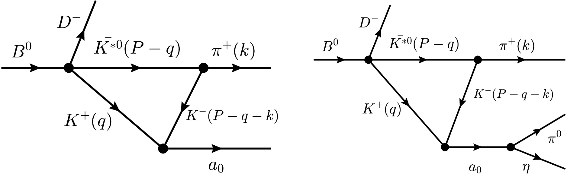
$ 1420\; \mathrm{MeV} $ , induced by the TS, can be generated in the$ B^0 \to D^- \pi^+ a_0(980) $ decay. The Feynman diagram is shown in the left panel of Fig. 1. In this process, the$ B^0 $ first decays into$ D^- \bar{K}^{*0} K^+ $ , after which the$ \bar{K}^{*0} $ decays into$ K^- $ and$ \pi^+ $ . The$ K^+ $ and$ K^- $ move in the same direction, with the$ K^- $ moving faster than the$ K^+ $ , allowing the$ K^+K^- $ pair to fuse into the$ a_0(980) $ . The channel$ B^0 \to D^{-} \bar{K}^{0} K^{*+} $ has not yet been observed experimentally. Therefore, the contribution of the$ K^{*+} $ -$ \bar{K}^{0} $ -$ K^{0} $ triangle loop from the$ B^0 \to D^{-} \bar{K}^{0} K^{*+} $ decay is not considered in the present work. Furthermore, the$ a_0(980) $ can be interpreted as a dynamically generated state with isospin$ I=1 $ , arising from the coupled channels$ \pi^0\eta $ ,$ K^+K^- $ , and$ K^0\bar{K}^0 $ within the chiral unitary approach [87, 88]. The decay of$ a_0(980) $ is shown in the right panel of Fig. 1.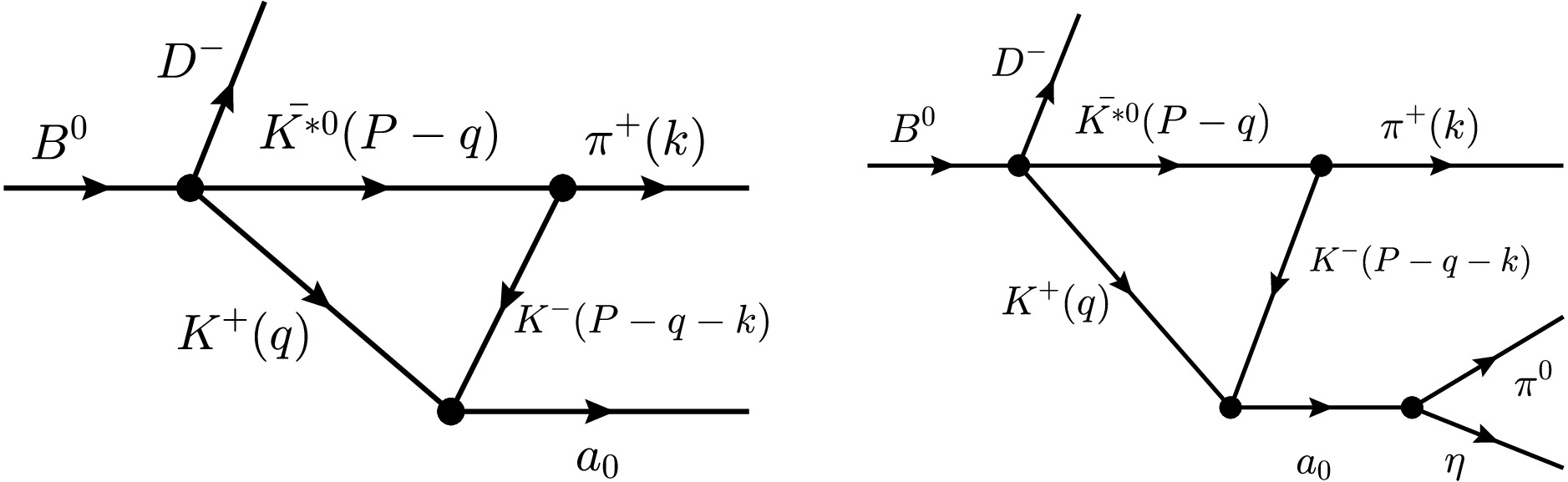
Figure 1. The Feynman diagrams for the
$ B^0 \to D^- \pi^+ a_0(980) $ and$ B^0 \to D^- \pi^+ a_0(980), a_0(980)\to\pi^0 \eta $ processes involving a$ \bar{K}^{*} $ -K-$ \bar{K} $ triangle loop are shown in the left and right panels, respectively.The TS occurs when the kinematic variables of the internal particles satisfy the following condition
$ \begin{aligned}[b] &\lim\limits_{\epsilon \to 0} \left( q_+^{\text{on}} -q_-^{\text{a}} \right)=0, \\& q_+^{\text{on}} =\frac{\lambda^{\tfrac{1}{2}}\left(m_{\text{inv}}^2(\pi a_0),m_{K}^2,m_{\bar{K}^{*0}}^2\right)}{2m_{\text{inv}}(\pi a_0)} + {\rm i} \epsilon, \end{aligned} $
(1) where
$ q_{+}^{\text{on}} $ denotes the on-shell three-momentum of$ K^{+} $ in the center-of-mass frame (COM) of the$ \bar{K}^{*0} K^+ $ system. The quantity$ m_{\text{inv}}(\pi a_0) $ is the invariant mass of the$ \bar{K}^{*0} K^+ $ system, and$ \lambda(x, y, z)=x^2 +y^2 +z^2 -2xy-2yz -2xz $ is the Källén function. Meanwhile,$ q_-^{\text{a}} $ is given by$ q_-^{\text{a}} =\gamma(\nu E_{K^-}^*-p_{K^-}^*)-{\rm i} \epsilon, $
(2) with the definitions
$ \begin{aligned}[b] &\nu = \frac{k}{E_{a_0}}, \qquad \gamma=\frac{1}{\sqrt{1-\nu^2}}=\frac{E_{a_0}}{m_{a_0}},\\& E_{K^-}^*= \frac{m_{a_0}}{2},\qquad p_{K^-}^*=\frac{\lambda^{\tfrac{1}{2}}(m_{a_0}^2,m_{K}^2,m_{K}^2)}{2m_{a_0}}, \end{aligned} $
(3) where
$ E_{K^{-}}^* $ and$ p_{K^{-}}^* $ are the energy and momentum of the$ K^{-} $ meson in the rest frame of$ a_0 $ . ν and γ denote the velocity of the$ K^+ K^- $ system and the Lorentz boost factor, respectively. Eq. (1) implies that all three particles in the loop are on shell and that$ K^+ $ in the rest frame of$ a_0(980) $ and$ a_0(980) $ in the COM frame of$ \pi a_0(980) $ move in the same direction. The formation of$ a_0(980) $ through$ K^+ K^- $ fusion further requires that the momentum of$ K^+ $ in the COM frame of$ \pi a_0 $ be smaller than that of$ K^- $ in the rest frame of$ \bar{K}^{*0} $ . Equivalently, Eq. (1) can be understood as the condition that$ q^a_- $ and$ q^{\text{on}}_+ $ represent the singularities of the triangle loop function in the upper and lower halves of the complex-q plane, respectively. The integration contour of the loop function in Eq. (21) is then pinched between$ q^a_- $ and$ q^{\text{on}}_+ $ at the same point on the real axis. Consequently, solving Eq. (1) yields a TS around$ 1420 $ MeV in the$ m_{\text{inv}}(\pi a_0) $ invariant mass distribution. When the finite width of the$ \bar{K}^{*0} $ is taken into account by replacing$m_{\bar{K}^{*0}} \to m_{\bar{K}^{*0}} - {\rm i}\Gamma_{\bar{K}^{*0}}/2$ with$ \Gamma_{\bar{K}^{*0}} = 47\; \mathrm{MeV} $ , the TS moves into the complex plane, yielding$1420.7 - {\rm i}\,28.0\; \mathrm{MeV}$ . -
In this section, we show that a peak structure around
$ 1420\; \mathrm{MeV} $ , induced by the TS, can be generated in the$ B^0 \to D^- \pi^+ a_0(980) $ decay. The Feynman diagram is shown in the left panel of Fig. 1. In this process, the$ B^0 $ first decays into$ D^- \bar{K}^{*0} K^+ $ , after which the$ \bar{K}^{*0} $ decays into$ K^- $ and$ \pi^+ $ . The$ K^+ $ and$ K^- $ move in the same direction, with the$ K^- $ moving faster than the$ K^+ $ , allowing the$ K^+K^- $ pair to fuse into the$ a_0(980) $ . The channel$ B^0 \to D^{-} \bar{K}^{0} K^{*+} $ has not yet been observed experimentally. Therefore, the contribution of the$ K^{*+} $ -$ \bar{K}^{0} $ -$ K^{0} $ triangle loop from the$ B^0 \to D^{-} \bar{K}^{0} K^{*+} $ decay is not considered in the present work. Furthermore, the$ a_0(980) $ can be interpreted as a dynamically generated state with isospin$ I=1 $ , arising from the coupled channels$ \pi^0\eta $ ,$ K^+K^- $ , and$ K^0\bar{K}^0 $ within the chiral unitary approach [87, 88]. The decay of$ a_0(980) $ is shown in the right panel of Fig. 1.
Figure 1. The Feynman diagrams for the
$ B^0 \to D^- \pi^+ a_0(980) $ and$ B^0 \to D^- \pi^+ a_0(980), a_0(980)\to\pi^0 \eta $ processes involving a$ \bar{K}^{*} $ -K-$ \bar{K} $ triangle loop are shown in the left and right panels, respectively.The TS occurs when the kinematic variables of the internal particles satisfy the following condition
$ \begin{aligned}[b] &\lim\limits_{\epsilon \to 0} \left( q_+^{\text{on}} -q_-^{\text{a}} \right)=0, \\& q_+^{\text{on}} =\frac{\lambda^{\tfrac{1}{2}}\left(m_{\text{inv}}^2(\pi a_0),m_{K}^2,m_{\bar{K}^{*0}}^2\right)}{2m_{\text{inv}}(\pi a_0)} + {\rm i} \epsilon, \end{aligned} $
(1) where
$ q_{+}^{\text{on}} $ denotes the on-shell three-momentum of$ K^{+} $ in the center-of-mass frame (COM) of the$ \bar{K}^{*0} K^+ $ system. The quantity$ m_{\text{inv}}(\pi a_0) $ is the invariant mass of the$ \bar{K}^{*0} K^+ $ system, and$ \lambda(x, y, z)=x^2 +y^2 +z^2 -2xy-2yz -2xz $ is the Källén function. Meanwhile,$ q_-^{\text{a}} $ is given by$ q_-^{\text{a}} =\gamma(\nu E_{K^-}^*-p_{K^-}^*)-{\rm i} \epsilon, $
(2) with the definitions
$ \begin{aligned}[b] &\nu = \frac{k}{E_{a_0}}, \qquad \gamma=\frac{1}{\sqrt{1-\nu^2}}=\frac{E_{a_0}}{m_{a_0}},\\& E_{K^-}^*= \frac{m_{a_0}}{2},\qquad p_{K^-}^*=\frac{\lambda^{\tfrac{1}{2}}(m_{a_0}^2,m_{K}^2,m_{K}^2)}{2m_{a_0}}, \end{aligned} $
(3) where
$ E_{K^{-}}^* $ and$ p_{K^{-}}^* $ are the energy and momentum of the$ K^{-} $ meson in the rest frame of$ a_0 $ . ν and γ denote the velocity of the$ K^+ K^- $ system and the Lorentz boost factor, respectively. Eq. (1) implies that all three particles in the loop are on shell and that$ K^+ $ in the rest frame of$ a_0(980) $ and$ a_0(980) $ in the COM frame of$ \pi a_0(980) $ move in the same direction. The formation of$ a_0(980) $ through$ K^+ K^- $ fusion further requires that the momentum of$ K^+ $ in the COM frame of$ \pi a_0 $ be smaller than that of$ K^- $ in the rest frame of$ \bar{K}^{*0} $ . Equivalently, Eq. (1) can be understood as the condition that$ q^a_- $ and$ q^{\text{on}}_+ $ represent the singularities of the triangle loop function in the upper and lower halves of the complex-q plane, respectively. The integration contour of the loop function in Eq. (21) is then pinched between$ q^a_- $ and$ q^{\text{on}}_+ $ at the same point on the real axis. Consequently, solving Eq. (1) yields a TS around$ 1420 $ MeV in the$ m_{\text{inv}}(\pi a_0) $ invariant mass distribution. When the finite width of the$ \bar{K}^{*0} $ is taken into account by replacing$m_{\bar{K}^{*0}} \to m_{\bar{K}^{*0}} - {\rm i}\Gamma_{\bar{K}^{*0}}/2$ with$ \Gamma_{\bar{K}^{*0}} = 47\; \mathrm{MeV} $ , the TS moves into the complex plane, yielding$1420.7 - {\rm i}\,28.0\; \mathrm{MeV}$ . -
In this section, we show that a peak structure around
$ 1420\; \mathrm{MeV} $ , induced by the TS, can be generated in the$ B^0 \to D^- \pi^+ a_0(980) $ decay. The Feynman diagram is shown in the left panel of Fig. 1. In this process, the$ B^0 $ first decays into$ D^- \bar{K}^{*0} K^+ $ , after which the$ \bar{K}^{*0} $ decays into$ K^- $ and$ \pi^+ $ . The$ K^+ $ and$ K^- $ move in the same direction, with the$ K^- $ moving faster than the$ K^+ $ , allowing the$ K^+K^- $ pair to fuse into the$ a_0(980) $ . The channel$ B^0 \to D^{-} \bar{K}^{0} K^{*+} $ has not yet been observed experimentally. Therefore, the contribution of the$ K^{*+} $ -$ \bar{K}^{0} $ -$ K^{0} $ triangle loop from the$ B^0 \to D^{-} \bar{K}^{0} K^{*+} $ decay is not considered in the present work. Furthermore, the$ a_0(980) $ can be interpreted as a dynamically generated state with isospin$ I=1 $ , arising from the coupled channels$ \pi^0\eta $ ,$ K^+K^- $ , and$ K^0\bar{K}^0 $ within the chiral unitary approach [87, 88]. The decay of$ a_0(980) $ is shown in the right panel of Fig. 1.
Figure 1. The Feynman diagrams for the
$ B^0 \to D^- \pi^+ a_0(980) $ and$ B^0 \to D^- \pi^+ a_0(980), a_0(980)\to\pi^0 \eta $ processes involving a$ \bar{K}^{*} $ -K-$ \bar{K} $ triangle loop are shown in the left and right panels, respectively.The TS occurs when the kinematic variables of the internal particles satisfy the following condition
$ \begin{aligned}[b] &\lim\limits_{\epsilon \to 0} \left( q_+^{\text{on}} -q_-^{\text{a}} \right)=0, \\& q_+^{\text{on}} =\frac{\lambda^{\tfrac{1}{2}}\left(m_{\text{inv}}^2(\pi a_0),m_{K}^2,m_{\bar{K}^{*0}}^2\right)}{2m_{\text{inv}}(\pi a_0)} + {\rm i} \epsilon, \end{aligned} $
(1) where
$ q_{+}^{\text{on}} $ denotes the on-shell three-momentum of$ K^{+} $ in the center-of-mass frame (COM) of the$ \bar{K}^{*0} K^+ $ system. The quantity$ m_{\text{inv}}(\pi a_0) $ is the invariant mass of the$ \bar{K}^{*0} K^+ $ system, and$ \lambda(x, y, z)=x^2 +y^2 +z^2 -2xy-2yz -2xz $ is the Källén function. Meanwhile,$ q_-^{\text{a}} $ is given by$ q_-^{\text{a}} =\gamma(\nu E_{K^-}^*-p_{K^-}^*)-{\rm i} \epsilon, $
(2) with the definitions
$ \begin{aligned}[b] &\nu = \frac{k}{E_{a_0}}, \qquad \gamma=\frac{1}{\sqrt{1-\nu^2}}=\frac{E_{a_0}}{m_{a_0}},\\& E_{K^-}^*= \frac{m_{a_0}}{2},\qquad p_{K^-}^*=\frac{\lambda^{\tfrac{1}{2}}(m_{a_0}^2,m_{K}^2,m_{K}^2)}{2m_{a_0}}, \end{aligned} $
(3) where
$ E_{K^{-}}^* $ and$ p_{K^{-}}^* $ are the energy and momentum of the$ K^{-} $ meson in the rest frame of$ a_0 $ . ν and γ denote the velocity of the$ K^+ K^- $ system and the Lorentz boost factor, respectively. Eq. (1) implies that all three particles in the loop are on shell and that$ K^+ $ in the rest frame of$ a_0(980) $ and$ a_0(980) $ in the COM frame of$ \pi a_0(980) $ move in the same direction. The formation of$ a_0(980) $ through$ K^+ K^- $ fusion further requires that the momentum of$ K^+ $ in the COM frame of$ \pi a_0 $ be smaller than that of$ K^- $ in the rest frame of$ \bar{K}^{*0} $ . Equivalently, Eq. (1) can be understood as the condition that$ q^a_- $ and$ q^{\text{on}}_+ $ represent the singularities of the triangle loop function in the upper and lower halves of the complex-q plane, respectively. The integration contour of the loop function in Eq. (21) is then pinched between$ q^a_- $ and$ q^{\text{on}}_+ $ at the same point on the real axis. Consequently, solving Eq. (1) yields a TS around$ 1420 $ MeV in the$ m_{\text{inv}}(\pi a_0) $ invariant mass distribution. When the finite width of the$ \bar{K}^{*0} $ is taken into account by replacing$m_{\bar{K}^{*0}} \to m_{\bar{K}^{*0}} - {\rm i}\Gamma_{\bar{K}^{*0}}/2$ with$ \Gamma_{\bar{K}^{*0}} = 47\; \mathrm{MeV} $ , the TS moves into the complex plane, yielding$1420.7 - {\rm i}\,28.0\; \mathrm{MeV}$ . -
In this section, we show that a peak structure around
$ 1420\; \mathrm{MeV} $ , induced by the TS, can be generated in the$ B^0 \to D^- \pi^+ a_0(980) $ decay. The Feynman diagram is shown in the left panel of Fig. 1. In this process, the$ B^0 $ first decays into$ D^- \bar{K}^{*0} K^+ $ , after which the$ \bar{K}^{*0} $ decays into$ K^- $ and$ \pi^+ $ . The$ K^+ $ and$ K^- $ move in the same direction, with the$ K^- $ moving faster than the$ K^+ $ , allowing the$ K^+K^- $ pair to fuse into the$ a_0(980) $ . The channel$ B^0 \to D^{-} \bar{K}^{0} K^{*+} $ has not yet been observed experimentally. Therefore, the contribution of the$ K^{*+} $ -$ \bar{K}^{0} $ -$ K^{0} $ triangle loop from the$ B^0 \to D^{-} \bar{K}^{0} K^{*+} $ decay is not considered in the present work. Furthermore, the$ a_0(980) $ can be interpreted as a dynamically generated state with isospin$ I=1 $ , arising from the coupled channels$ \pi^0\eta $ ,$ K^+K^- $ , and$ K^0\bar{K}^0 $ within the chiral unitary approach [87, 88]. The decay of$ a_0(980) $ is shown in the right panel of Fig. 1.
Figure 1. The Feynman diagrams for the
$ B^0 \to D^- \pi^+ a_0(980) $ and$ B^0 \to D^- \pi^+ a_0(980), a_0(980)\to\pi^0 \eta $ processes involving a$ \bar{K}^{*} $ -K-$ \bar{K} $ triangle loop are shown in the left and right panels, respectively.The TS occurs when the kinematic variables of the internal particles satisfy the following condition
$ \begin{aligned}[b] &\lim\limits_{\epsilon \to 0} \left( q_+^{\text{on}} -q_-^{\text{a}} \right)=0, \\& q_+^{\text{on}} =\frac{\lambda^{\tfrac{1}{2}}\left(m_{\text{inv}}^2(\pi a_0),m_{K}^2,m_{\bar{K}^{*0}}^2\right)}{2m_{\text{inv}}(\pi a_0)} + {\rm i} \epsilon, \end{aligned} $
(1) where
$ q_{+}^{\text{on}} $ denotes the on-shell three-momentum of$ K^{+} $ in the center-of-mass frame (COM) of the$ \bar{K}^{*0} K^+ $ system. The quantity$ m_{\text{inv}}(\pi a_0) $ is the invariant mass of the$ \bar{K}^{*0} K^+ $ system, and$ \lambda(x, y, z)=x^2 +y^2 +z^2 -2xy-2yz -2xz $ is the Källén function. Meanwhile,$ q_-^{\text{a}} $ is given by$ q_-^{\text{a}} =\gamma(\nu E_{K^-}^*-p_{K^-}^*)-{\rm i} \epsilon, $
(2) with the definitions
$ \begin{aligned}[b] &\nu = \frac{k}{E_{a_0}}, \qquad \gamma=\frac{1}{\sqrt{1-\nu^2}}=\frac{E_{a_0}}{m_{a_0}},\\& E_{K^-}^*= \frac{m_{a_0}}{2},\qquad p_{K^-}^*=\frac{\lambda^{\tfrac{1}{2}}(m_{a_0}^2,m_{K}^2,m_{K}^2)}{2m_{a_0}}, \end{aligned} $
(3) where
$ E_{K^{-}}^* $ and$ p_{K^{-}}^* $ are the energy and momentum of the$ K^{-} $ meson in the rest frame of$ a_0 $ . ν and γ denote the velocity of the$ K^+ K^- $ system and the Lorentz boost factor, respectively. Eq. (1) implies that all three particles in the loop are on shell and that$ K^+ $ in the rest frame of$ a_0(980) $ and$ a_0(980) $ in the COM frame of$ \pi a_0(980) $ move in the same direction. The formation of$ a_0(980) $ through$ K^+ K^- $ fusion further requires that the momentum of$ K^+ $ in the COM frame of$ \pi a_0 $ be smaller than that of$ K^- $ in the rest frame of$ \bar{K}^{*0} $ . Equivalently, Eq. (1) can be understood as the condition that$ q^a_- $ and$ q^{\text{on}}_+ $ represent the singularities of the triangle loop function in the upper and lower halves of the complex-q plane, respectively. The integration contour of the loop function in Eq. (21) is then pinched between$ q^a_- $ and$ q^{\text{on}}_+ $ at the same point on the real axis. Consequently, solving Eq. (1) yields a TS around$ 1420 $ MeV in the$ m_{\text{inv}}(\pi a_0) $ invariant mass distribution. When the finite width of the$ \bar{K}^{*0} $ is taken into account by replacing$m_{\bar{K}^{*0}} \to m_{\bar{K}^{*0}} - {\rm i}\Gamma_{\bar{K}^{*0}}/2$ with$ \Gamma_{\bar{K}^{*0}} = 47\; \mathrm{MeV} $ , the TS moves into the complex plane, yielding$1420.7 - {\rm i}\,28.0\; \mathrm{MeV}$ . -
In this section, we show that a peak structure around
$ 1420\; \mathrm{MeV} $ , induced by the TS, can be generated in the$ B^0 \to D^- \pi^+ a_0(980) $ decay. The Feynman diagram is shown in the left panel of Fig. 1. In this process, the$ B^0 $ first decays into$ D^- \bar{K}^{*0} K^+ $ , after which the$ \bar{K}^{*0} $ decays into$ K^- $ and$ \pi^+ $ . The$ K^+ $ and$ K^- $ move in the same direction, with the$ K^- $ moving faster than the$ K^+ $ , allowing the$ K^+K^- $ pair to fuse into the$ a_0(980) $ . The channel$ B^0 \to D^{-} \bar{K}^{0} K^{*+} $ has not yet been observed experimentally. Therefore, the contribution of the$ K^{*+} $ -$ \bar{K}^{0} $ -$ K^{0} $ triangle loop from the$ B^0 \to D^{-} \bar{K}^{0} K^{*+} $ decay is not considered in the present work. Furthermore, the$ a_0(980) $ can be interpreted as a dynamically generated state with isospin$ I=1 $ , arising from the coupled channels$ \pi^0\eta $ ,$ K^+K^- $ , and$ K^0\bar{K}^0 $ within the chiral unitary approach [87, 88]. The decay of$ a_0(980) $ is shown in the right panel of Fig. 1.
Figure 1. The Feynman diagrams for the
$ B^0 \to D^- \pi^+ a_0(980) $ and$ B^0 \to D^- \pi^+ a_0(980), a_0(980)\to\pi^0 \eta $ processes involving a$ \bar{K}^{*} $ -K-$ \bar{K} $ triangle loop are shown in the left and right panels, respectively.The TS occurs when the kinematic variables of the internal particles satisfy the following condition
$ \begin{aligned}[b] &\lim\limits_{\epsilon \to 0} \left( q_+^{\text{on}} -q_-^{\text{a}} \right)=0, \\& q_+^{\text{on}} =\frac{\lambda^{\tfrac{1}{2}}\left(m_{\text{inv}}^2(\pi a_0),m_{K}^2,m_{\bar{K}^{*0}}^2\right)}{2m_{\text{inv}}(\pi a_0)} + {\rm i} \epsilon, \end{aligned} $
(1) where
$ q_{+}^{\text{on}} $ denotes the on-shell three-momentum of$ K^{+} $ in the center-of-mass frame (COM) of the$ \bar{K}^{*0} K^+ $ system. The quantity$ m_{\text{inv}}(\pi a_0) $ is the invariant mass of the$ \bar{K}^{*0} K^+ $ system, and$ \lambda(x, y, z)=x^2 +y^2 +z^2 -2xy-2yz -2xz $ is the Källén function. Meanwhile,$ q_-^{\text{a}} $ is given by$ q_-^{\text{a}} =\gamma(\nu E_{K^-}^*-p_{K^-}^*)-{\rm i} \epsilon, $
(2) with the definitions
$ \begin{aligned}[b] &\nu = \frac{k}{E_{a_0}}, \qquad \gamma=\frac{1}{\sqrt{1-\nu^2}}=\frac{E_{a_0}}{m_{a_0}},\\& E_{K^-}^*= \frac{m_{a_0}}{2},\qquad p_{K^-}^*=\frac{\lambda^{\tfrac{1}{2}}(m_{a_0}^2,m_{K}^2,m_{K}^2)}{2m_{a_0}}, \end{aligned} $
(3) where
$ E_{K^{-}}^* $ and$ p_{K^{-}}^* $ are the energy and momentum of the$ K^{-} $ meson in the rest frame of$ a_0 $ . ν and γ denote the velocity of the$ K^+ K^- $ system and the Lorentz boost factor, respectively. Eq. (1) implies that all three particles in the loop are on shell and that$ K^+ $ in the rest frame of$ a_0(980) $ and$ a_0(980) $ in the COM frame of$ \pi a_0(980) $ move in the same direction. The formation of$ a_0(980) $ through$ K^+ K^- $ fusion further requires that the momentum of$ K^+ $ in the COM frame of$ \pi a_0 $ be smaller than that of$ K^- $ in the rest frame of$ \bar{K}^{*0} $ . Equivalently, Eq. (1) can be understood as the condition that$ q^a_- $ and$ q^{\text{on}}_+ $ represent the singularities of the triangle loop function in the upper and lower halves of the complex-q plane, respectively. The integration contour of the loop function in Eq. (21) is then pinched between$ q^a_- $ and$ q^{\text{on}}_+ $ at the same point on the real axis. Consequently, solving Eq. (1) yields a TS around$ 1420 $ MeV in the$ m_{\text{inv}}(\pi a_0) $ invariant mass distribution. When the finite width of the$ \bar{K}^{*0} $ is taken into account by replacing$m_{\bar{K}^{*0}} \to m_{\bar{K}^{*0}} - {\rm i}\Gamma_{\bar{K}^{*0}}/2$ with$ \Gamma_{\bar{K}^{*0}} = 47\; \mathrm{MeV} $ , the TS moves into the complex plane, yielding$1420.7 - {\rm i}\,28.0\; \mathrm{MeV}$ . -
In this section, we show that a peak structure around
$ 1420\; \mathrm{MeV} $ , induced by the TS, can be generated in the$ B^0 \to D^- \pi^+ a_0(980) $ decay. The Feynman diagram is shown in the left panel of Fig. 1. In this process, the$ B^0 $ first decays into$ D^- \bar{K}^{*0} K^+ $ , after which the$ \bar{K}^{*0} $ decays into$ K^- $ and$ \pi^+ $ . The$ K^+ $ and$ K^- $ move in the same direction, with the$ K^- $ moving faster than the$ K^+ $ , allowing the$ K^+K^- $ pair to fuse into the$ a_0(980) $ . The channel$ B^0 \to D^{-} \bar{K}^{0} K^{*+} $ has not yet been observed experimentally. Therefore, the contribution of the$ K^{*+} $ -$ \bar{K}^{0} $ -$ K^{0} $ triangle loop from the$ B^0 \to D^{-} \bar{K}^{0} K^{*+} $ decay is not considered in the present work. Furthermore, the$ a_0(980) $ can be interpreted as a dynamically generated state with isospin$ I=1 $ , arising from the coupled channels$ \pi^0\eta $ ,$ K^+K^- $ , and$ K^0\bar{K}^0 $ within the chiral unitary approach [87, 88]. The decay of$ a_0(980) $ is shown in the right panel of Fig. 1.
Figure 1. The Feynman diagrams for the
$ B^0 \to D^- \pi^+ a_0(980) $ and$ B^0 \to D^- \pi^+ a_0(980), a_0(980)\to\pi^0 \eta $ processes involving a$ \bar{K}^{*} $ -K-$ \bar{K} $ triangle loop are shown in the left and right panels, respectively.The TS occurs when the kinematic variables of the internal particles satisfy the following condition
$ \begin{aligned}[b] &\lim\limits_{\epsilon \to 0} \left( q_+^{\text{on}} -q_-^{\text{a}} \right)=0, \\& q_+^{\text{on}} =\frac{\lambda^{\tfrac{1}{2}}\left(m_{\text{inv}}^2(\pi a_0),m_{K}^2,m_{\bar{K}^{*0}}^2\right)}{2m_{\text{inv}}(\pi a_0)} + {\rm i} \epsilon, \end{aligned} $
(1) where
$ q_{+}^{\text{on}} $ denotes the on-shell three-momentum of$ K^{+} $ in the center-of-mass frame (COM) of the$ \bar{K}^{*0} K^+ $ system. The quantity$ m_{\text{inv}}(\pi a_0) $ is the invariant mass of the$ \bar{K}^{*0} K^+ $ system, and$ \lambda(x, y, z)=x^2 +y^2 +z^2 -2xy-2yz -2xz $ is the Källén function. Meanwhile,$ q_-^{\text{a}} $ is given by$ q_-^{\text{a}} =\gamma(\nu E_{K^-}^*-p_{K^-}^*)-{\rm i} \epsilon, $
(2) with the definitions
$ \begin{aligned}[b] &\nu = \frac{k}{E_{a_0}}, \qquad \gamma=\frac{1}{\sqrt{1-\nu^2}}=\frac{E_{a_0}}{m_{a_0}},\\& E_{K^-}^*= \frac{m_{a_0}}{2},\qquad p_{K^-}^*=\frac{\lambda^{\tfrac{1}{2}}(m_{a_0}^2,m_{K}^2,m_{K}^2)}{2m_{a_0}}, \end{aligned} $
(3) where
$ E_{K^{-}}^* $ and$ p_{K^{-}}^* $ are the energy and momentum of the$ K^{-} $ meson in the rest frame of$ a_0 $ . ν and γ denote the velocity of the$ K^+ K^- $ system and the Lorentz boost factor, respectively. Eq. (1) implies that all three particles in the loop are on shell and that$ K^+ $ in the rest frame of$ a_0(980) $ and$ a_0(980) $ in the COM frame of$ \pi a_0(980) $ move in the same direction. The formation of$ a_0(980) $ through$ K^+ K^- $ fusion further requires that the momentum of$ K^+ $ in the COM frame of$ \pi a_0 $ be smaller than that of$ K^- $ in the rest frame of$ \bar{K}^{*0} $ . Equivalently, Eq. (1) can be understood as the condition that$ q^a_- $ and$ q^{\text{on}}_+ $ represent the singularities of the triangle loop function in the upper and lower halves of the complex-q plane, respectively. The integration contour of the loop function in Eq. (21) is then pinched between$ q^a_- $ and$ q^{\text{on}}_+ $ at the same point on the real axis. Consequently, solving Eq. (1) yields a TS around$ 1420 $ MeV in the$ m_{\text{inv}}(\pi a_0) $ invariant mass distribution. When the finite width of the$ \bar{K}^{*0} $ is taken into account by replacing$m_{\bar{K}^{*0}} \to m_{\bar{K}^{*0}} - {\rm i}\Gamma_{\bar{K}^{*0}}/2$ with$ \Gamma_{\bar{K}^{*0}} = 47\; \mathrm{MeV} $ , the TS moves into the complex plane, yielding$1420.7 - {\rm i}\,28.0\; \mathrm{MeV}$ . -
To evaluate the amplitude shown in Fig. 1, the effective coupling strength of the
$ B^0 \to D^- K^+ \bar{K}^{*0} $ vertex is required. The$ B^0 $ meson can decay into the$ D^- K^+ \bar{K}^{*0} $ final state through the weak decay of the b quark, as illustrated in Fig. 2. At the quark level, the b quark undergoes a weak transition into a c quark through the emission of a W boson and hadronizes into the$ D^- $ meson. The emitted W boson subsequently decays into a$ u\bar{d} $ pair, which combines with an additional$ q\bar{q} $ pair from the vacuum to form the$ \bar{K}^{*0}K^+ $ final state.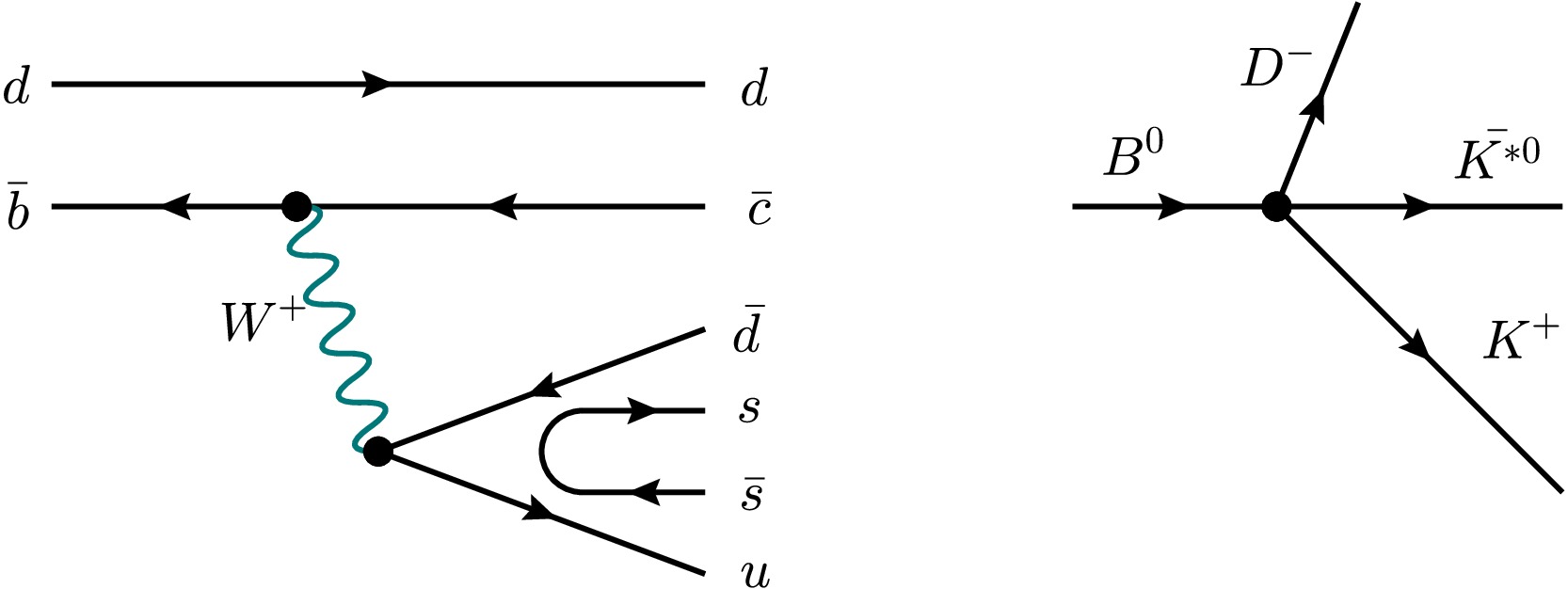
Figure 2. (color online) The quark-level and hadron-level Feynman diagrams for the decay
$ B^0 \to D^- K^+ \bar{K}^{*0} $ are shown in the left and right panels, respectively.The interaction of the effective vertex in Fig. 2 can be constructed using the P-wave interaction. Following the convention adopted in Refs. [28, 53], we write
$ -{\rm i}t_{B \to D K \bar{K}^{*0}}=-{\rm i}C \vec{\epsilon}_{\bar{K}^{*0}} \cdot \vec{p}_{D}, $
(4) where
$ \vec{\epsilon}_{\bar{K}^{*0}} $ and$ \vec{p}_{D} $ are the polarization vector of the$ \bar{K}^{*0} $ and the momentum of the$ D^- $ , respectively. Below, we present the details of the calculation of the vertex coupling strength C. By solving Eq. (1), a TS around$1420\; \mathrm{MeV}$ is obtained. The three-momentum of the$ \bar{K}^{*0} $ in the$ \pi a_0 $ rest frame is approximately$ 135.66\; \mathrm{MeV} $ , which is smaller than the$ \bar{K}^{*0} $ mass of$ 895.81 $ MeV. Therefore, the time component$ \epsilon^0 $ of the$ \bar{K}^{*0} $ polarization vector can be safely neglected. We take the polarization sum for the$ \bar{K}^{*0} $ as$ \begin{aligned}[b] &\displaystyle\sum\limits_{\mu, \nu} \epsilon_{\bar{K}^{*0}\mu}\epsilon_{\bar{K}^{*0}\nu} \sim \displaystyle\sum\limits_{i,j} \epsilon_{\bar{K}^{*0}i}\epsilon_{\bar{K}^{*0}j}=\delta_{ij}; \\& \;\;\;\; \mu=i,\ \mu=j;\qquad i,j=1,2,3. \end{aligned} $
(5) The decay width for the process
$ B \to D K \bar{K}^{*0} $ is given by$ \begin{aligned}[b] \Gamma_{B \to D K \bar{K}^{*0}} =&\int {\rm d} m_{\text{inv}}( \bar{K}^{*0} K^+) \\& \times \frac{1}{(2\pi)^3}\frac{|\vec{\tilde{p}}_{D} | |\vec{\tilde{p}}^\prime_{\bar{K}^{*0}} | }{4m_{B}^2} \displaystyle\sum\limits_{\text{pol}}|t_{B \to D K \bar{K}^{*0}}|^2, \end{aligned} $
(6) where
$ m_{\mathrm{inv}}(\bar{K}^{*0}K^+) $ is the invariant mass of the$ \bar{K}^{*0}K^+ $ system. Here,$ \vec{\tilde{p}}^{\,\prime}_{\bar{K}^{*0}} $ and$ \vec{\tilde{p}}_{D} $ denote the three-momenta of the$ \bar{K}^{*0} $ in the$ \bar{K}^{*0}K^+ $ COM frame and of the$ D^- $ in the$ B^0 $ rest frame, respectively. They are given by$ \begin{aligned}[b] &|\vec{\tilde{p}}_{D} | =\frac{\lambda^{\tfrac{1}{2}}\left(m^2_{B},\ m_{\text{inv}}^2( \bar{K}^{*0} K^+),\ m^2_{D} \right)}{2 m_{B}}, \\& |\vec{\tilde{p}}^\prime_{\bar{K}^{*0}} | =\frac{\lambda^{\tfrac{1}{2}}\left(m_{\text{inv}}^2( \bar{K}^{*0} K^+),\ m^2_{K},\ m^2_{\bar{K}^{*0}}\right)}{2 m_{\text{inv}}( \bar{K}^{*0} K^+ )}. \end{aligned} $
(7) After squaring the amplitude
$ t_{B \to D K \bar{K}^{*0} } $ and applying the polarization sum in Eq. (5), we obtain$ \sum \limits_{\text{pol}} |t_{B \to D K \bar{K}^{*0}}|^2=C^2 |\vec{\tilde{p}}_{D}^\prime|^2, $
(8) where
$ \vec{\tilde{p}}_{D}^\prime $ is the three-momentum of the$ D^- $ in the COM frame of the$ \bar{K}^{*0}K^+ $ system.$ |\vec{\tilde{p}}_{D}^\prime |=\frac{\lambda^{\tfrac{1}{2}}\left(m^2_{B},\ m_{\text{inv}}^2( \bar{K}^{*0} K^+),\ m^2_{D} \right)}{2 m_{\text{inv}}( \bar{K}^{*0} K^+)}. $
(9) From recent measurements [1, 85], the partial decay branching fraction is given by Br(
$ B^0 \to D^- K^+ \bar{K}^{*0} $ ) =$ (7.7\pm 0.6)\times 10^{-4} $ . Combining Eq. (6) with Eq. (8), we obtain$ \frac{C^2}{\Gamma_{B^0}}=\frac{\text{Br} \left( B^0 \to D^- K^+ \bar{K}^{*0}\right) }{\displaystyle\int {\rm d} m_{\text{inv}}( \bar{K}^{*0} K^+)\dfrac{1}{(2\pi)^3}\dfrac{ |\vec{\tilde{p}}_{D} | |\vec{\tilde{p}}^\prime_{\bar{K}^{*0}} |}{4m_{B}^2} |\vec{\tilde{p}}_{D}^\prime|^2}. $
(10) -
To evaluate the amplitude shown in Fig. 1, the effective coupling strength of the
$ B^0 \to D^- K^+ \bar{K}^{*0} $ vertex is required. The$ B^0 $ meson can decay into the$ D^- K^+ \bar{K}^{*0} $ final state through the weak decay of the b quark, as illustrated in Fig. 2. At the quark level, the b quark undergoes a weak transition into a c quark through the emission of a W boson and hadronizes into the$ D^- $ meson. The emitted W boson subsequently decays into a$ u\bar{d} $ pair, which combines with an additional$ q\bar{q} $ pair from the vacuum to form the$ \bar{K}^{*0}K^+ $ final state.
Figure 2. (color online) The quark-level and hadron-level Feynman diagrams for the decay
$ B^0 \to D^- K^+ \bar{K}^{*0} $ are shown in the left and right panels, respectively.The interaction of the effective vertex in Fig. 2 can be constructed using the P-wave interaction. Following the convention adopted in Refs. [28, 53], we write
$ -{\rm i}t_{B \to D K \bar{K}^{*0}}=-{\rm i}C \vec{\epsilon}_{\bar{K}^{*0}} \cdot \vec{p}_{D}, $
(4) where
$ \vec{\epsilon}_{\bar{K}^{*0}} $ and$ \vec{p}_{D} $ are the polarization vector of the$ \bar{K}^{*0} $ and the momentum of the$ D^- $ , respectively. Below, we present the details of the calculation of the vertex coupling strength C. By solving Eq. (1), a TS around$1420\; \mathrm{MeV}$ is obtained. The three-momentum of the$ \bar{K}^{*0} $ in the$ \pi a_0 $ rest frame is approximately$ 135.66\; \mathrm{MeV} $ , which is smaller than the$ \bar{K}^{*0} $ mass of$ 895.81 $ MeV. Therefore, the time component$ \epsilon^0 $ of the$ \bar{K}^{*0} $ polarization vector can be safely neglected. We take the polarization sum for the$ \bar{K}^{*0} $ as$ \begin{aligned}[b] &\displaystyle\sum\limits_{\mu, \nu} \epsilon_{\bar{K}^{*0}\mu}\epsilon_{\bar{K}^{*0}\nu} \sim \displaystyle\sum\limits_{i,j} \epsilon_{\bar{K}^{*0}i}\epsilon_{\bar{K}^{*0}j}=\delta_{ij}; \\& \;\;\;\; \mu=i,\ \mu=j;\qquad i,j=1,2,3. \end{aligned} $
(5) The decay width for the process
$ B \to D K \bar{K}^{*0} $ is given by$ \begin{aligned}[b] \Gamma_{B \to D K \bar{K}^{*0}} =&\int {\rm d} m_{\text{inv}}( \bar{K}^{*0} K^+) \\& \times \frac{1}{(2\pi)^3}\frac{|\vec{\tilde{p}}_{D} | |\vec{\tilde{p}}^\prime_{\bar{K}^{*0}} | }{4m_{B}^2} \displaystyle\sum\limits_{\text{pol}}|t_{B \to D K \bar{K}^{*0}}|^2, \end{aligned} $
(6) where
$ m_{\mathrm{inv}}(\bar{K}^{*0}K^+) $ is the invariant mass of the$ \bar{K}^{*0}K^+ $ system. Here,$ \vec{\tilde{p}}^{\,\prime}_{\bar{K}^{*0}} $ and$ \vec{\tilde{p}}_{D} $ denote the three-momenta of the$ \bar{K}^{*0} $ in the$ \bar{K}^{*0}K^+ $ COM frame and of the$ D^- $ in the$ B^0 $ rest frame, respectively. They are given by$ \begin{aligned}[b] &|\vec{\tilde{p}}_{D} | =\frac{\lambda^{\tfrac{1}{2}}\left(m^2_{B},\ m_{\text{inv}}^2( \bar{K}^{*0} K^+),\ m^2_{D} \right)}{2 m_{B}}, \\& |\vec{\tilde{p}}^\prime_{\bar{K}^{*0}} | =\frac{\lambda^{\tfrac{1}{2}}\left(m_{\text{inv}}^2( \bar{K}^{*0} K^+),\ m^2_{K},\ m^2_{\bar{K}^{*0}}\right)}{2 m_{\text{inv}}( \bar{K}^{*0} K^+ )}. \end{aligned} $
(7) After squaring the amplitude
$ t_{B \to D K \bar{K}^{*0} } $ and applying the polarization sum in Eq. (5), we obtain$ \sum \limits_{\text{pol}} |t_{B \to D K \bar{K}^{*0}}|^2=C^2 |\vec{\tilde{p}}_{D}^\prime|^2, $
(8) where
$ \vec{\tilde{p}}_{D}^\prime $ is the three-momentum of the$ D^- $ in the COM frame of the$ \bar{K}^{*0}K^+ $ system.$ |\vec{\tilde{p}}_{D}^\prime |=\frac{\lambda^{\tfrac{1}{2}}\left(m^2_{B},\ m_{\text{inv}}^2( \bar{K}^{*0} K^+),\ m^2_{D} \right)}{2 m_{\text{inv}}( \bar{K}^{*0} K^+)}. $
(9) From recent measurements [1, 85], the partial decay branching fraction is given by Br(
$ B^0 \to D^- K^+ \bar{K}^{*0} $ ) =$ (7.7\pm 0.6)\times 10^{-4} $ . Combining Eq. (6) with Eq. (8), we obtain$ \frac{C^2}{\Gamma_{B^0}}=\frac{\text{Br} \left( B^0 \to D^- K^+ \bar{K}^{*0}\right) }{\displaystyle\int {\rm d} m_{\text{inv}}( \bar{K}^{*0} K^+)\dfrac{1}{(2\pi)^3}\dfrac{ |\vec{\tilde{p}}_{D} | |\vec{\tilde{p}}^\prime_{\bar{K}^{*0}} |}{4m_{B}^2} |\vec{\tilde{p}}_{D}^\prime|^2}. $
(10) -
To evaluate the amplitude shown in Fig. 1, the effective coupling strength of the
$ B^0 \to D^- K^+ \bar{K}^{*0} $ vertex is required. The$ B^0 $ meson can decay into the$ D^- K^+ \bar{K}^{*0} $ final state through the weak decay of the b quark, as illustrated in Fig. 2. At the quark level, the b quark undergoes a weak transition into a c quark through the emission of a W boson and hadronizes into the$ D^- $ meson. The emitted W boson subsequently decays into a$ u\bar{d} $ pair, which combines with an additional$ q\bar{q} $ pair from the vacuum to form the$ \bar{K}^{*0}K^+ $ final state.
Figure 2. (color online) The quark-level and hadron-level Feynman diagrams for the decay
$ B^0 \to D^- K^+ \bar{K}^{*0} $ are shown in the left and right panels, respectively.The interaction of the effective vertex in Fig. 2 can be constructed using the P-wave interaction. Following the convention adopted in Refs. [28, 53], we write
$ -{\rm i}t_{B \to D K \bar{K}^{*0}}=-{\rm i}C \vec{\epsilon}_{\bar{K}^{*0}} \cdot \vec{p}_{D}, $
(4) where
$ \vec{\epsilon}_{\bar{K}^{*0}} $ and$ \vec{p}_{D} $ are the polarization vector of the$ \bar{K}^{*0} $ and the momentum of the$ D^- $ , respectively. Below, we present the details of the calculation of the vertex coupling strength C. By solving Eq. (1), a TS around$1420\; \mathrm{MeV}$ is obtained. The three-momentum of the$ \bar{K}^{*0} $ in the$ \pi a_0 $ rest frame is approximately$ 135.66\; \mathrm{MeV} $ , which is smaller than the$ \bar{K}^{*0} $ mass of$ 895.81 $ MeV. Therefore, the time component$ \epsilon^0 $ of the$ \bar{K}^{*0} $ polarization vector can be safely neglected. We take the polarization sum for the$ \bar{K}^{*0} $ as$ \begin{aligned}[b] &\displaystyle\sum\limits_{\mu, \nu} \epsilon_{\bar{K}^{*0}\mu}\epsilon_{\bar{K}^{*0}\nu} \sim \displaystyle\sum\limits_{i,j} \epsilon_{\bar{K}^{*0}i}\epsilon_{\bar{K}^{*0}j}=\delta_{ij}; \\& \;\;\;\; \mu=i,\ \mu=j;\qquad i,j=1,2,3. \end{aligned} $
(5) The decay width for the process
$ B \to D K \bar{K}^{*0} $ is given by$ \begin{aligned}[b] \Gamma_{B \to D K \bar{K}^{*0}} =&\int {\rm d} m_{\text{inv}}( \bar{K}^{*0} K^+) \\& \times \frac{1}{(2\pi)^3}\frac{|\vec{\tilde{p}}_{D} | |\vec{\tilde{p}}^\prime_{\bar{K}^{*0}} | }{4m_{B}^2} \displaystyle\sum\limits_{\text{pol}}|t_{B \to D K \bar{K}^{*0}}|^2, \end{aligned} $
(6) where
$ m_{\mathrm{inv}}(\bar{K}^{*0}K^+) $ is the invariant mass of the$ \bar{K}^{*0}K^+ $ system. Here,$ \vec{\tilde{p}}^{\,\prime}_{\bar{K}^{*0}} $ and$ \vec{\tilde{p}}_{D} $ denote the three-momenta of the$ \bar{K}^{*0} $ in the$ \bar{K}^{*0}K^+ $ COM frame and of the$ D^- $ in the$ B^0 $ rest frame, respectively. They are given by$ \begin{aligned}[b] &|\vec{\tilde{p}}_{D} | =\frac{\lambda^{\tfrac{1}{2}}\left(m^2_{B},\ m_{\text{inv}}^2( \bar{K}^{*0} K^+),\ m^2_{D} \right)}{2 m_{B}}, \\& |\vec{\tilde{p}}^\prime_{\bar{K}^{*0}} | =\frac{\lambda^{\tfrac{1}{2}}\left(m_{\text{inv}}^2( \bar{K}^{*0} K^+),\ m^2_{K},\ m^2_{\bar{K}^{*0}}\right)}{2 m_{\text{inv}}( \bar{K}^{*0} K^+ )}. \end{aligned} $
(7) After squaring the amplitude
$ t_{B \to D K \bar{K}^{*0} } $ and applying the polarization sum in Eq. (5), we obtain$ \sum \limits_{\text{pol}} |t_{B \to D K \bar{K}^{*0}}|^2=C^2 |\vec{\tilde{p}}_{D}^\prime|^2, $
(8) where
$ \vec{\tilde{p}}_{D}^\prime $ is the three-momentum of the$ D^- $ in the COM frame of the$ \bar{K}^{*0}K^+ $ system.$ |\vec{\tilde{p}}_{D}^\prime |=\frac{\lambda^{\tfrac{1}{2}}\left(m^2_{B},\ m_{\text{inv}}^2( \bar{K}^{*0} K^+),\ m^2_{D} \right)}{2 m_{\text{inv}}( \bar{K}^{*0} K^+)}. $
(9) From recent measurements [1, 85], the partial decay branching fraction is given by Br(
$ B^0 \to D^- K^+ \bar{K}^{*0} $ ) =$ (7.7\pm 0.6)\times 10^{-4} $ . Combining Eq. (6) with Eq. (8), we obtain$ \frac{C^2}{\Gamma_{B^0}}=\frac{\text{Br} \left( B^0 \to D^- K^+ \bar{K}^{*0}\right) }{\displaystyle\int {\rm d} m_{\text{inv}}( \bar{K}^{*0} K^+)\dfrac{1}{(2\pi)^3}\dfrac{ |\vec{\tilde{p}}_{D} | |\vec{\tilde{p}}^\prime_{\bar{K}^{*0}} |}{4m_{B}^2} |\vec{\tilde{p}}_{D}^\prime|^2}. $
(10) -
To evaluate the amplitude shown in Fig. 1, the effective coupling strength of the
$ B^0 \to D^- K^+ \bar{K}^{*0} $ vertex is required. The$ B^0 $ meson can decay into the$ D^- K^+ \bar{K}^{*0} $ final state through the weak decay of the b quark, as illustrated in Fig. 2. At the quark level, the b quark undergoes a weak transition into a c quark through the emission of a W boson and hadronizes into the$ D^- $ meson. The emitted W boson subsequently decays into a$ u\bar{d} $ pair, which combines with an additional$ q\bar{q} $ pair from the vacuum to form the$ \bar{K}^{*0}K^+ $ final state.
Figure 2. (color online) The quark-level and hadron-level Feynman diagrams for the decay
$ B^0 \to D^- K^+ \bar{K}^{*0} $ are shown in the left and right panels, respectively.The interaction of the effective vertex in Fig. 2 can be constructed using the P-wave interaction. Following the convention adopted in Refs. [28, 53], we write
$ -{\rm i}t_{B \to D K \bar{K}^{*0}}=-{\rm i}C \vec{\epsilon}_{\bar{K}^{*0}} \cdot \vec{p}_{D}, $
(4) where
$ \vec{\epsilon}_{\bar{K}^{*0}} $ and$ \vec{p}_{D} $ are the polarization vector of the$ \bar{K}^{*0} $ and the momentum of the$ D^- $ , respectively. Below, we present the details of the calculation of the vertex coupling strength C. By solving Eq. (1), a TS around$1420\; \mathrm{MeV}$ is obtained. The three-momentum of the$ \bar{K}^{*0} $ in the$ \pi a_0 $ rest frame is approximately$ 135.66\; \mathrm{MeV} $ , which is smaller than the$ \bar{K}^{*0} $ mass of$ 895.81 $ MeV. Therefore, the time component$ \epsilon^0 $ of the$ \bar{K}^{*0} $ polarization vector can be safely neglected. We take the polarization sum for the$ \bar{K}^{*0} $ as$ \begin{aligned}[b] &\displaystyle\sum\limits_{\mu, \nu} \epsilon_{\bar{K}^{*0}\mu}\epsilon_{\bar{K}^{*0}\nu} \sim \displaystyle\sum\limits_{i,j} \epsilon_{\bar{K}^{*0}i}\epsilon_{\bar{K}^{*0}j}=\delta_{ij}; \\& \;\;\;\; \mu=i,\ \mu=j;\qquad i,j=1,2,3. \end{aligned} $
(5) The decay width for the process
$ B \to D K \bar{K}^{*0} $ is given by$ \begin{aligned}[b] \Gamma_{B \to D K \bar{K}^{*0}} =&\int {\rm d} m_{\text{inv}}( \bar{K}^{*0} K^+) \\& \times \frac{1}{(2\pi)^3}\frac{|\vec{\tilde{p}}_{D} | |\vec{\tilde{p}}^\prime_{\bar{K}^{*0}} | }{4m_{B}^2} \displaystyle\sum\limits_{\text{pol}}|t_{B \to D K \bar{K}^{*0}}|^2, \end{aligned} $
(6) where
$ m_{\mathrm{inv}}(\bar{K}^{*0}K^+) $ is the invariant mass of the$ \bar{K}^{*0}K^+ $ system. Here,$ \vec{\tilde{p}}^{\,\prime}_{\bar{K}^{*0}} $ and$ \vec{\tilde{p}}_{D} $ denote the three-momenta of the$ \bar{K}^{*0} $ in the$ \bar{K}^{*0}K^+ $ COM frame and of the$ D^- $ in the$ B^0 $ rest frame, respectively. They are given by$ \begin{aligned}[b] &|\vec{\tilde{p}}_{D} | =\frac{\lambda^{\tfrac{1}{2}}\left(m^2_{B},\ m_{\text{inv}}^2( \bar{K}^{*0} K^+),\ m^2_{D} \right)}{2 m_{B}}, \\& |\vec{\tilde{p}}^\prime_{\bar{K}^{*0}} | =\frac{\lambda^{\tfrac{1}{2}}\left(m_{\text{inv}}^2( \bar{K}^{*0} K^+),\ m^2_{K},\ m^2_{\bar{K}^{*0}}\right)}{2 m_{\text{inv}}( \bar{K}^{*0} K^+ )}. \end{aligned} $
(7) After squaring the amplitude
$ t_{B \to D K \bar{K}^{*0} } $ and applying the polarization sum in Eq. (5), we obtain$ \sum \limits_{\text{pol}} |t_{B \to D K \bar{K}^{*0}}|^2=C^2 |\vec{\tilde{p}}_{D}^\prime|^2, $
(8) where
$ \vec{\tilde{p}}_{D}^\prime $ is the three-momentum of the$ D^- $ in the COM frame of the$ \bar{K}^{*0}K^+ $ system.$ |\vec{\tilde{p}}_{D}^\prime |=\frac{\lambda^{\tfrac{1}{2}}\left(m^2_{B},\ m_{\text{inv}}^2( \bar{K}^{*0} K^+),\ m^2_{D} \right)}{2 m_{\text{inv}}( \bar{K}^{*0} K^+)}. $
(9) From recent measurements [1, 85], the partial decay branching fraction is given by Br(
$ B^0 \to D^- K^+ \bar{K}^{*0} $ ) =$ (7.7\pm 0.6)\times 10^{-4} $ . Combining Eq. (6) with Eq. (8), we obtain$ \frac{C^2}{\Gamma_{B^0}}=\frac{\text{Br} \left( B^0 \to D^- K^+ \bar{K}^{*0}\right) }{\displaystyle\int {\rm d} m_{\text{inv}}( \bar{K}^{*0} K^+)\dfrac{1}{(2\pi)^3}\dfrac{ |\vec{\tilde{p}}_{D} | |\vec{\tilde{p}}^\prime_{\bar{K}^{*0}} |}{4m_{B}^2} |\vec{\tilde{p}}_{D}^\prime|^2}. $
(10) -
To evaluate the amplitude shown in Fig. 1, the effective coupling strength of the
$ B^0 \to D^- K^+ \bar{K}^{*0} $ vertex is required. The$ B^0 $ meson can decay into the$ D^- K^+ \bar{K}^{*0} $ final state through the weak decay of the b quark, as illustrated in Fig. 2. At the quark level, the b quark undergoes a weak transition into a c quark through the emission of a W boson and hadronizes into the$ D^- $ meson. The emitted W boson subsequently decays into a$ u\bar{d} $ pair, which combines with an additional$ q\bar{q} $ pair from the vacuum to form the$ \bar{K}^{*0}K^+ $ final state.
Figure 2. (color online) The quark-level and hadron-level Feynman diagrams for the decay
$ B^0 \to D^- K^+ \bar{K}^{*0} $ are shown in the left and right panels, respectively.The interaction of the effective vertex in Fig. 2 can be constructed using the P-wave interaction. Following the convention adopted in Refs. [28, 53], we write
$ -{\rm i}t_{B \to D K \bar{K}^{*0}}=-{\rm i}C \vec{\epsilon}_{\bar{K}^{*0}} \cdot \vec{p}_{D}, $
(4) where
$ \vec{\epsilon}_{\bar{K}^{*0}} $ and$ \vec{p}_{D} $ are the polarization vector of the$ \bar{K}^{*0} $ and the momentum of the$ D^- $ , respectively. Below, we present the details of the calculation of the vertex coupling strength C. By solving Eq. (1), a TS around$1420\; \mathrm{MeV}$ is obtained. The three-momentum of the$ \bar{K}^{*0} $ in the$ \pi a_0 $ rest frame is approximately$ 135.66\; \mathrm{MeV} $ , which is smaller than the$ \bar{K}^{*0} $ mass of$ 895.81 $ MeV. Therefore, the time component$ \epsilon^0 $ of the$ \bar{K}^{*0} $ polarization vector can be safely neglected. We take the polarization sum for the$ \bar{K}^{*0} $ as$ \begin{aligned}[b] &\displaystyle\sum\limits_{\mu, \nu} \epsilon_{\bar{K}^{*0}\mu}\epsilon_{\bar{K}^{*0}\nu} \sim \displaystyle\sum\limits_{i,j} \epsilon_{\bar{K}^{*0}i}\epsilon_{\bar{K}^{*0}j}=\delta_{ij}; \\& \;\;\;\; \mu=i,\ \mu=j;\qquad i,j=1,2,3. \end{aligned} $
(5) The decay width for the process
$ B \to D K \bar{K}^{*0} $ is given by$ \begin{aligned}[b] \Gamma_{B \to D K \bar{K}^{*0}} =&\int {\rm d} m_{\text{inv}}( \bar{K}^{*0} K^+) \\& \times \frac{1}{(2\pi)^3}\frac{|\vec{\tilde{p}}_{D} | |\vec{\tilde{p}}^\prime_{\bar{K}^{*0}} | }{4m_{B}^2} \displaystyle\sum\limits_{\text{pol}}|t_{B \to D K \bar{K}^{*0}}|^2, \end{aligned} $
(6) where
$ m_{\mathrm{inv}}(\bar{K}^{*0}K^+) $ is the invariant mass of the$ \bar{K}^{*0}K^+ $ system. Here,$ \vec{\tilde{p}}^{\,\prime}_{\bar{K}^{*0}} $ and$ \vec{\tilde{p}}_{D} $ denote the three-momenta of the$ \bar{K}^{*0} $ in the$ \bar{K}^{*0}K^+ $ COM frame and of the$ D^- $ in the$ B^0 $ rest frame, respectively. They are given by$ \begin{aligned}[b] &|\vec{\tilde{p}}_{D} | =\frac{\lambda^{\tfrac{1}{2}}\left(m^2_{B},\ m_{\text{inv}}^2( \bar{K}^{*0} K^+),\ m^2_{D} \right)}{2 m_{B}}, \\& |\vec{\tilde{p}}^\prime_{\bar{K}^{*0}} | =\frac{\lambda^{\tfrac{1}{2}}\left(m_{\text{inv}}^2( \bar{K}^{*0} K^+),\ m^2_{K},\ m^2_{\bar{K}^{*0}}\right)}{2 m_{\text{inv}}( \bar{K}^{*0} K^+ )}. \end{aligned} $
(7) After squaring the amplitude
$ t_{B \to D K \bar{K}^{*0} } $ and applying the polarization sum in Eq. (5), we obtain$ \sum \limits_{\text{pol}} |t_{B \to D K \bar{K}^{*0}}|^2=C^2 |\vec{\tilde{p}}_{D}^\prime|^2, $
(8) where
$ \vec{\tilde{p}}_{D}^\prime $ is the three-momentum of the$ D^- $ in the COM frame of the$ \bar{K}^{*0}K^+ $ system.$ |\vec{\tilde{p}}_{D}^\prime |=\frac{\lambda^{\tfrac{1}{2}}\left(m^2_{B},\ m_{\text{inv}}^2( \bar{K}^{*0} K^+),\ m^2_{D} \right)}{2 m_{\text{inv}}( \bar{K}^{*0} K^+)}. $
(9) From recent measurements [1, 85], the partial decay branching fraction is given by Br(
$ B^0 \to D^- K^+ \bar{K}^{*0} $ ) =$ (7.7\pm 0.6)\times 10^{-4} $ . Combining Eq. (6) with Eq. (8), we obtain$ \frac{C^2}{\Gamma_{B^0}}=\frac{\text{Br} \left( B^0 \to D^- K^+ \bar{K}^{*0}\right) }{\displaystyle\int {\rm d} m_{\text{inv}}( \bar{K}^{*0} K^+)\dfrac{1}{(2\pi)^3}\dfrac{ |\vec{\tilde{p}}_{D} | |\vec{\tilde{p}}^\prime_{\bar{K}^{*0}} |}{4m_{B}^2} |\vec{\tilde{p}}_{D}^\prime|^2}. $
(10) -
To evaluate the amplitude shown in Fig. 1, the effective coupling strength of the
$ B^0 \to D^- K^+ \bar{K}^{*0} $ vertex is required. The$ B^0 $ meson can decay into the$ D^- K^+ \bar{K}^{*0} $ final state through the weak decay of the b quark, as illustrated in Fig. 2. At the quark level, the b quark undergoes a weak transition into a c quark through the emission of a W boson and hadronizes into the$ D^- $ meson. The emitted W boson subsequently decays into a$ u\bar{d} $ pair, which combines with an additional$ q\bar{q} $ pair from the vacuum to form the$ \bar{K}^{*0}K^+ $ final state.
Figure 2. (color online) The quark-level and hadron-level Feynman diagrams for the decay
$ B^0 \to D^- K^+ \bar{K}^{*0} $ are shown in the left and right panels, respectively.The interaction of the effective vertex in Fig. 2 can be constructed using the P-wave interaction. Following the convention adopted in Refs. [28, 53], we write
$ -{\rm i}t_{B \to D K \bar{K}^{*0}}=-{\rm i}C \vec{\epsilon}_{\bar{K}^{*0}} \cdot \vec{p}_{D}, $
(4) where
$ \vec{\epsilon}_{\bar{K}^{*0}} $ and$ \vec{p}_{D} $ are the polarization vector of the$ \bar{K}^{*0} $ and the momentum of the$ D^- $ , respectively. Below, we present the details of the calculation of the vertex coupling strength C. By solving Eq. (1), a TS around$1420\; \mathrm{MeV}$ is obtained. The three-momentum of the$ \bar{K}^{*0} $ in the$ \pi a_0 $ rest frame is approximately$ 135.66\; \mathrm{MeV} $ , which is smaller than the$ \bar{K}^{*0} $ mass of$ 895.81 $ MeV. Therefore, the time component$ \epsilon^0 $ of the$ \bar{K}^{*0} $ polarization vector can be safely neglected. We take the polarization sum for the$ \bar{K}^{*0} $ as$ \begin{aligned}[b] &\displaystyle\sum\limits_{\mu, \nu} \epsilon_{\bar{K}^{*0}\mu}\epsilon_{\bar{K}^{*0}\nu} \sim \displaystyle\sum\limits_{i,j} \epsilon_{\bar{K}^{*0}i}\epsilon_{\bar{K}^{*0}j}=\delta_{ij}; \\& \;\;\;\; \mu=i,\ \mu=j;\qquad i,j=1,2,3. \end{aligned} $
(5) The decay width for the process
$ B \to D K \bar{K}^{*0} $ is given by$ \begin{aligned}[b] \Gamma_{B \to D K \bar{K}^{*0}} =&\int {\rm d} m_{\text{inv}}( \bar{K}^{*0} K^+) \\& \times \frac{1}{(2\pi)^3}\frac{|\vec{\tilde{p}}_{D} | |\vec{\tilde{p}}^\prime_{\bar{K}^{*0}} | }{4m_{B}^2} \displaystyle\sum\limits_{\text{pol}}|t_{B \to D K \bar{K}^{*0}}|^2, \end{aligned} $
(6) where
$ m_{\mathrm{inv}}(\bar{K}^{*0}K^+) $ is the invariant mass of the$ \bar{K}^{*0}K^+ $ system. Here,$ \vec{\tilde{p}}^{\,\prime}_{\bar{K}^{*0}} $ and$ \vec{\tilde{p}}_{D} $ denote the three-momenta of the$ \bar{K}^{*0} $ in the$ \bar{K}^{*0}K^+ $ COM frame and of the$ D^- $ in the$ B^0 $ rest frame, respectively. They are given by$ \begin{aligned}[b] &|\vec{\tilde{p}}_{D} | =\frac{\lambda^{\tfrac{1}{2}}\left(m^2_{B},\ m_{\text{inv}}^2( \bar{K}^{*0} K^+),\ m^2_{D} \right)}{2 m_{B}}, \\& |\vec{\tilde{p}}^\prime_{\bar{K}^{*0}} | =\frac{\lambda^{\tfrac{1}{2}}\left(m_{\text{inv}}^2( \bar{K}^{*0} K^+),\ m^2_{K},\ m^2_{\bar{K}^{*0}}\right)}{2 m_{\text{inv}}( \bar{K}^{*0} K^+ )}. \end{aligned} $
(7) After squaring the amplitude
$ t_{B \to D K \bar{K}^{*0} } $ and applying the polarization sum in Eq. (5), we obtain$ \sum \limits_{\text{pol}} |t_{B \to D K \bar{K}^{*0}}|^2=C^2 |\vec{\tilde{p}}_{D}^\prime|^2, $
(8) where
$ \vec{\tilde{p}}_{D}^\prime $ is the three-momentum of the$ D^- $ in the COM frame of the$ \bar{K}^{*0}K^+ $ system.$ |\vec{\tilde{p}}_{D}^\prime |=\frac{\lambda^{\tfrac{1}{2}}\left(m^2_{B},\ m_{\text{inv}}^2( \bar{K}^{*0} K^+),\ m^2_{D} \right)}{2 m_{\text{inv}}( \bar{K}^{*0} K^+)}. $
(9) From recent measurements [1, 85], the partial decay branching fraction is given by Br(
$ B^0 \to D^- K^+ \bar{K}^{*0} $ ) =$ (7.7\pm 0.6)\times 10^{-4} $ . Combining Eq. (6) with Eq. (8), we obtain$ \frac{C^2}{\Gamma_{B^0}}=\frac{\text{Br} \left( B^0 \to D^- K^+ \bar{K}^{*0}\right) }{\displaystyle\int {\rm d} m_{\text{inv}}( \bar{K}^{*0} K^+)\dfrac{1}{(2\pi)^3}\dfrac{ |\vec{\tilde{p}}_{D} | |\vec{\tilde{p}}^\prime_{\bar{K}^{*0}} |}{4m_{B}^2} |\vec{\tilde{p}}_{D}^\prime|^2}. $
(10) -
The amplitude for the
$ B^0 \to D^- \pi^+ a_0(980) $ decay (left panel of Fig. 1) can be written as$ \begin{aligned}[b] -{\rm i} t_{B \to D \pi a_0}=& {\rm i} \displaystyle\sum\limits_{\text{pol}} \displaystyle\int \frac{{\rm d}^4 q}{(2\pi)^4}\ \frac{{\rm i} t_{B \to D K \bar{K}^{*0}}}{q^2-m_{K}^2+ {\rm i} \epsilon}\\& \times\frac{{\rm i} t_{\bar{K}^{*0} K^- \pi^+}}{(P-q)^2-m_{\bar{K}^{*0}}^2+ {\rm i} \epsilon}\ \frac{{\rm i} t_{K^+ K^- a_0 } }{(P-q-k)^2-m_{K}^2+ {\rm i} \epsilon}, \end{aligned} $
(11) in the COM frame of the
$ \pi a_0 $ system, where the$ \pi^+ $ originates from the$ \bar{K}^{*0} $ decay. In Eq. (11), the amplitude$ t_{B \to D K \bar{K}^{*0}} $ was calculated in the previous section (Sec. III). The amplitude$ t_{\bar{K}^{*0} K^- \pi^+} $ can be calculated using the chiral-invariant Lagrangian with local hidden symmetry [89, 90] and is given by$ {\cal{L}}_{\text{VPP}}=-{\rm i} g\langle V^\mu[P,\partial_\mu P]\rangle, $
(12) where bracket
$ \langle \cdots \rangle $ denotes the SU(3) trace, and the coupling constant is given by$ g=m_V/2f_\pi $ , with$ m_V=800 $ MeV and$ f_\pi=93 $ MeV, within the local hidden gauge formalism. P and$ V^\mu $ represent the pseudoscalar and vector meson octets, respectively, which are given by$ \begin{aligned}[b] P=\begin{pmatrix} \dfrac{\pi^0}{\sqrt{2}}+\dfrac{\eta_8}{\sqrt{6}} &\pi^+ &K^+\\ \pi^-&-\dfrac{\pi^0}{\sqrt{2}}+\dfrac{\eta_8}{\sqrt{6}} &K^0\\ K^-& \bar{K}^0& -\dfrac{2}{\sqrt{6}}\eta_8 \end{pmatrix} , \\ V=\begin{pmatrix} \dfrac{\rho^0}{\sqrt{2}}+\dfrac{\omega}{\sqrt{2}}& \rho^+& K^{*+}\\ \rho^-&-\dfrac{\rho^0}{\sqrt{2}}+\dfrac{\omega}{\sqrt{2}} & K^{*0}\\ K^{*-}& \bar{K}^{*0}& \phi \end{pmatrix} . \end{aligned} $
(13) Then, the amplitude for the decay
$ \bar{K}^{*0} \to K^- \pi^+ $ can be written as$ -{\rm i} t_{\bar{K}^{*0} K^- \pi^+}=-{\rm i} g\vec{\epsilon}_{\bar{K}^{*0}} \cdot (\vec{p}_{\pi^+}^{\,\prime}-\vec{p}_{K^-}^{\,\prime}). $
(14) As in Eq. (8), we neglect the time component of the polarization vector in Eq. (14) and employ the polarization sum given in Eq. (5). Here,
$ \vec{p}_{\pi^+}^{\,\prime} $ and$ \vec{p}_{K^-}^{\,\prime} $ denote the three-momenta of the$ \pi^+ $ and$ K^- $ in the COM frame of the$ \pi a_0 $ system, respectively. The momentum$ \vec{p}_{\pi^+}^{\,\prime} $ is given by$ |\vec{p}_{\pi^+}^{\,\prime}| =|\vec{k}|=\frac{\lambda^{\tfrac{1}{2}}\left(m^2_{\text{inv}}(\pi a_0),\ m_{\pi}^2,\ m^2_{a_0} \right)}{2 m_{\text{inv}}(\pi a_0)}. $
(15) As discussed in Sec. II, the
$ a_0(980) $ is considered to be a dynamically generated state. The amplitude$ t_{K^+ K^- a_0 } $ can be written directly as$ t_{K^+ K^- a_0 }=g_{K^+ K^- a_0 }. $
(16) Above, we set
$ g_{K^+ K^- a_0 } = 3875 $ MeV [87]. Thus, the amplitude expression in Eq. (11) can be simplified to$ \begin{aligned}[b] t_{B \to D \pi a_0 (980)}=& {\rm i} g_{K^+ K^- a_0 } g C \displaystyle\sum\limits_{\text{pol}} \int \frac{{\rm d}^4 q}{(2\pi)^4} \\&\times \frac{\vec{\epsilon}_{\bar{K}^{*0}} \cdot \vec{p}_{D}^{\,\prime} }{q^2-m_{K}^2+ {\rm i} \epsilon} \frac{\vec{\epsilon}_{\bar{K}^{*0}} \cdot (\vec{p}_{\pi^+}^{\,\prime}-\vec{p}_{K^-}^{\,\prime}) }{(P-q)^2-m_{\bar{K}^{*0}}^2+ {\rm i} \epsilon} \\& \times\frac{1}{(P-q-k)^2-m_{K}^2+ {\rm i} \epsilon} , \end{aligned} $
(17) where
$ \vec{p}_{\pi^+}^{\,\prime} $ is given in Eq. (15). The quantity$ \vec{p}_{D}^{\,\prime} $ is the momentum of the$ D^- $ in the COM frame of$ \pi a_0 $ , which originates from the$ B^0 $ decay.$ |\vec{p}_{D}^{\,\prime}|=\frac{\lambda^{\tfrac{1}{2}}\left(m^2_{B},\ m_{\text{inv}}^2( \pi a_0),\ m^2_{D} \right)}{2 m_{\text{inv}}( \pi a_0)}. $
(18) Equation (5) is used to perform the polarization sum in Eq. (17), yielding
$ \begin{aligned}[b] t_{B \to D \pi a_0 (980)} =& {\rm i} g_{K^+ K^- a_0 } g C \displaystyle\int \frac{{\rm d}^4 q}{(2\pi)^4} \\& \times\frac{1 }{q^2-m_{K}^2+ {\rm i} \epsilon} \frac{\vec{p}_{D}^{\,\prime} \cdot (2\vec{k}+\vec{q}) }{(P-q)^2-m_{\bar{K}^{*0}}^2+ {\rm i} \epsilon} \\&\times \frac{1}{(P-q-k)^2-m_{K}^2+ {\rm i} \epsilon}, \end{aligned} $
(19) where
$ \vec{p}_{\pi^+}^{\,\prime}-\vec{p}_{K^-}^{\,\prime}=\vec{k}-(-\vec{k}-\vec{q})=2\vec{k}+\vec{q} $ . P is the momentum of the$ \pi a_0 $ system in its rest frame.$ P=\left(m_{\text{inv}}(\pi a_0),\ 0,\ 0,\ 0 \right). $
(20) The quantity
$ t_T $ is defined to describe the loop integral in Eq. (19) as$ \begin{aligned}[b] t_T=& {\rm i}\displaystyle\int \frac{{\rm d}^4 q}{(2\pi)^4} \ \vec{p}_{D}^{\,\prime} \cdot (2\vec{k}+\vec{q})\frac{1 }{q^2-m_{K}^2+ {\rm i} \epsilon} \\& \times\frac{1 }{(P-q)^2-m_{\bar{K}^{*0}}^2+ {\rm i} \epsilon} \frac{1}{(P-q-k)^2-m_{K}^2+ {\rm i} \epsilon}. \end{aligned} $
(21) Following Refs. [24, 32], the negative-energy part of the
$ \bar{K}^{*0} $ propagator in$ t_T $ can be neglected. The integration over$ dq^0 $ in$ t_T $ is performed by applying the residue theorem and using the following formula$ \int {\rm d}^3q \ \vec{q}_i\ f(\vec{q},\vec{k})=\vec{k}_i \int {\rm d}^3 q \frac{\vec{q}\cdot \vec{k}}{|\vec{k}|^2} f(\vec{q},\vec{k}). $
(22) Now, the triangle loop amplitude
$ t_T $ reduces to$ \begin{aligned}[b] t_T =& \vec{p}_{D}^{\,\prime} \cdot \vec{k} \int \frac{{\rm d}^3 q}{(2\pi)^3} {\left(2+ \frac{\vec{q}\cdot \vec{k}}{|\vec{k}|^2}\right) }\\&\times \frac{1}{8\omega_{K^+}(\vec{q})\ \omega_{K^-}(\vec{q}+\vec{k})\ \omega_{K^*}(\vec{q})}\\ & \times\frac{1}{k^0 - \omega_{K^-}(\vec{q}+\vec{k}) - \omega_{K^*}(\vec{q}) + {\rm i}\epsilon}\\ & \times\frac{1}{P^0 - \omega_{K^*}(\vec{q}) - \omega_{K^+}(\vec{q}) + {\rm i}\epsilon}\\ & \times\frac{1}{P^0 - \omega_{K^+}(\vec{q}) - \omega_{K^-}(\vec{q}+\vec{k}) - k^0+ {\rm i}\epsilon}\\ & \times\frac{1}{P^0 + \omega_{K^+}(\vec{q}) + \omega_{K^-}(\vec{q}+\vec{k}) - k^0 + {\rm i} \epsilon} \end{aligned} $
$ \begin{aligned}[b] & \times\bigg\{ 2P^0\omega_{K^+}(\vec{q}) + 2k^0 \omega_{K^-}(\vec{q}+\vec{k}) \\ &- 2\left[ \omega_{K^+}(\vec{q}) + \omega_{K^-}(\vec{q}+\vec{k})\right] \\ & \times\left[ \omega_{K^+}(\vec{q}) + \omega_{K^-}(\vec{q}+\vec{k}) + \omega_{K^*}(\vec{q})\right] \bigg\},\\&= \vec{p}_{D}^{\,\prime} \cdot \vec{k} \times \tilde{t}_T, \end{aligned} $
(23) where
$ \omega_{K^+}(\vec{q})=\sqrt{m_{K}^2 + \vec{q}^2} $ ,$ \omega_{K^{*0}}(\vec{q})= \sqrt{m_{\bar{K}^{*0}}^2 + \vec{q}^2} $ , and$ \omega_{K^-}(\vec{q}+\vec{k}) = \sqrt{m_{K}^2 + (\vec{k}+\vec{q})^2} $ . From Eq. (20),$ P^0 = m_{\mathrm{inv}}(\pi a_0) $ is the invariant mass of the$ \pi a_0 $ system. Although the integral in Eq. (23) is convergent, the chiral unitary approach naturally provides an upper limit$ q_{\mathrm{max}} $ [10, 13]. In this work, we use$ q_{\mathrm{max}} = 600\; \mathrm{MeV} $ for$ a_0(980) $ production [86, 91]. To reproduce the peak observed in experiments, the finite width of the$ \bar{K}^{*0} $ in the triangle loop must be taken into account. This is implemented by replacing$ \omega_{K^{*}} $ with$\omega_{K^{*}} - {\rm i} \Gamma_{\bar{K}^{*0}}/2$ in the denominator of Eq. (23).Finally, the differential decay width for the three-body final state
$ B^0 \to D^- \pi^+ a_0(980) $ is given by$ \begin{aligned}[b] \frac{{\rm d} \Gamma^\prime}{{\rm d} m_{\text{inv}}(\pi a_0)} =&{\frac{2}{3}}\frac{1}{(2\pi)^3}\frac{ C^2g_{K^+ K^- a_0 }^2 g^2}{{8}m_{B}^2} \\ & \times {|\vec{p}_{D}| |\vec{p}_{D}^{\,\prime}|^2 |\vec{k}|^3 |\tilde{t}_T|^2}. \end{aligned} $
(24) The factor
$ 2/3 $ in Eq. (24) originates from the angular phase-space integration of the integrand in$ \vec{p}_{D}^{\,\prime} \cdot \vec{k}= |\vec{p}_{D}^{\,\prime}| | \vec{k}|\cos \theta $ . Here,$ \vec{p}_{D} $ denotes the momentum of the$ D^- $ in the$ B^0 $ rest frame.$ |\vec{p}_{D}|=\frac{\lambda^{\tfrac{1}{2}}\left(m_{B}^2,M_{D^-}^2,m_{\text{inv}}^2(\pi a_0) \right)}{2m_{B}}. $
(25) In addition, we further explore the possibility of observing the
$ a_0(980) $ through the$ \pi^0 \eta $ final state. Following Ref. [53], the$ a_0(980) $ appears as an unstable resonance in the$ B^0 $ decay and subsequently decays into$ \pi^0 \eta $ . Therefore, we consider the corresponding four-body decay, as illustrated in the right panel of Fig. 1. In this process, the$ a_0(980) $ resonance can be treated as an intermediate particle, allowing us to include an additional differential distribution with respect to the$ \pi\eta $ invariant mass in Eq. 24. The differential decay width for$ B^0 \to D^- \pi^+ \pi^0 \eta $ is then given by$\begin{aligned}[b] \frac{{\rm d} \Gamma^\prime}{{\rm d} m_{\text{inv}}(\pi a_0)} =&\frac{1}{3}\frac{1}{(2\pi)^3} \frac{g^2 C^2}{4m_{B}^2} \int {\rm d} m_{\text{inv}}^2(\pi \eta) \\ & \times \left(-\frac{1}{\pi}\text{Im}D \right) g_{K^- K^+ a_0}^2 {|\vec{p}_{D}| |\vec{p}_{D}^{\,\prime}|^2 |\vec{k}|^3 |\tilde{t}_T|^2}, \end{aligned} $
(26) with
$ D=\frac{1}{m_{\text{inv}}^2(\pi \eta)-m_{a_0}^2+{\rm i} m_{a_0}\Gamma_{a_0}}, $
(27) where
$ m_{\text{inv}}(\pi \eta) $ is the invariant mass of the$ \pi \eta $ system produced in the$ a_0(980) $ decay, and$ m_{a_0} $ is the mass of$ a_0(980) $ . Eq. (26) reduces to Eq. (24) in the limit$ \Gamma_{a_0} \to 0 $ , where${\rm i}\,\mathrm{Im}\,D \to -{\rm i}\pi \, \delta\big(m_{\mathrm{inv}}^2(\pi \eta) - m_{a_0}^2 \big)$ . Thus, Eq. (26) simplifies to$ \begin{aligned}[b] \frac{{\rm d} \Gamma^\prime}{{\rm d} m_{\text{inv}}(\pi a_0)} =&\frac{1}{3 \pi}\frac{1}{(2\pi)^3} \frac{g^2 C^2}{4m_{B}^2} \int {\rm d}m_{\text{inv}}^2(\pi \eta)\\ & \times \frac{g_{K^- K^+ a_0}^2 {|\vec{p}_{D}| |\vec{p}_{D}^{\,\prime}|^2 |\vec{k}|^3 |\tilde{t}_T|^2} m_{a_0} \Gamma_{a_0}}{\left[m_{\text{inv}}^2(\pi \eta)-m_{a_0}^2 \right]^2+(m_{a_0} \Gamma_{a_0})^2}. \end{aligned} $
(28) The decay width
$ \Gamma_{a_0} $ is calculated by considering the$ a_0 \to \pi^0 \eta $ decay$ \Gamma_{a_0} =\frac{1}{8\pi}\frac{g_{a_0 \pi \eta}^2}{m_{\text{inv}}^2(\pi \eta)}|\vec{\tilde{q}}_{\eta}|, $
(29) where
$ |\vec{\tilde{q}}_{\eta}| $ denotes the magnitude of the η momentum in the rest frame of$ a_0(980) $ and is given by$ |\vec{\tilde{q}}_{\eta}|= \frac{\lambda^{\tfrac{1}{2}}\left( m_{\text{inv}}^2(\pi \eta),m_\pi^2,m_\eta^2\right)}{2m_{\text{inv}}(\pi \eta)}. $
(30) By substituting Eq. (29) into Eq. (28), we obtain
$ \begin{aligned}[b]\frac{{\rm d} \Gamma^\prime}{{\rm d} m_{\text{inv}}(\pi a_0)} =&\frac{1}{(2\pi)^5} \frac{g^2 C^2}{24 m_{B}^2} \int {\rm d} m_{\text{inv}}^2(\pi \eta)\\ &\times {|\vec{p}_{D}| |\vec{p}_{D}^{\,\prime}|^2 |\vec{k}|^3 |\tilde{t}_T|^2} \frac{|\vec{\tilde{q}}_{\eta}|}{m_{\text{inv}}^2(\pi \eta)} \\ &\times \frac{m_{a_0} g_{K^- K^+ a_0}^2 g_{a_0 \pi \eta}^2}{\left[m_{\text{inv}}^2(\pi \eta)-m_{a_0}^2 \right]^2+(m_{a_0} \Gamma_{a_0})^2}. \end{aligned} $
(31) Meanwhile, the amplitude for the
$ K^+ K^- \to \pi \eta $ process mediated by exchange of the$ a_0(980) $ resonance can be written as$ \frac{g_{K^- K^+ a_0}^2 g_{a_0 \pi \eta}^2}{\left[m_{\text{inv}}^2(\pi \eta)-m_{a_0}^2 \right]^2+(m_{a_0} \Gamma_{a_0})^2}=|t_{K^+ K^-\to \pi \eta}|^2. $
(32) In contrast, when the
$ a_0(980) $ is treated as a dynamically generated state, the amplitude$ t_{K^+ K^-\to \pi \eta} $ can be calculated by solving the Bethe–Salpeter (BS) equation within the chiral unitary approach. The BS equation is given by$ T=\left[1-VG \right]^{-1}V. $
(33) Here, G denotes the loop function for two meson propagators [86].
$ G(s) = {\rm i}\int \frac{{\rm d}^4 q}{(2\pi)^4} \frac{1}{(P-q)^2-m_1^2+ {\rm i} \epsilon} \frac{1}{q^2-m_2^2+ {\rm i} \epsilon}, $
(34) and is regularized by a cutoff
$ q_{\text{max}} $ as$ \begin{aligned}[b] G(s) =& \frac{1}{16\pi^2 s} \Bigg\lbrace \sigma \left( \arctan \frac{s + \Delta}{\sigma \lambda_1} + \arctan \frac{s - \Delta}{\sigma \lambda_2} \right) \\&- \left[ (s + \Delta) \ln \frac{(1 + \lambda_1) q_{\text{max}}}{m_1} + (s - \Delta) \ln \frac{(1 + \lambda_2) q_{\text{max}}}{m_2} \right] \Bigg\rbrace, \end{aligned}$
with
$ \begin{aligned}[b] \sigma =\; &\left[-(s-(m_1+m_2)^2)(s-(m_1-m_2)^2)\right]^{1/2},\\ \Delta =\; & m_1^2-m_2^2, \;\; \lambda_1=\sqrt{1+\frac{m_1^2}{q^2_{\text{max}}}}, \;\; \lambda_2=\sqrt{1+\frac{m_2^2}{q^2_{\text{max}}}} \; . \end{aligned} $
A value of
$ q_{\text{max}}=600 $ MeV is used to reproduce the$ a_0(980) $ around 980 MeV. The meson-meson interaction potentials for the case$ I=1 $ are given as follows [86]:$ \begin{aligned}[b] &V_{K^+K^-\to K^+K^-} = -\frac{1}{2f_\pi^2}s, \quad V_{K^+K^-\to K^{0}\bar{K}^{0}} = -\frac{1}{4f_\pi^2}s,\\ & V_{K^+K^-\to\pi^{0}\eta} = \frac{- \sqrt{3}}{12f_\pi^2} \left( 3s - \frac{8}{3}m_K^2 - \frac{1}{3}m_{\pi}^2 - m_{\eta}^2 \right), \\& V_{K^{0}\bar{K}^{0}\to K^{0}\bar{K}^{0}} = -\frac{1}{2f_\pi^2}s, \quad V_{\pi^{0}\eta\to\pi^{0}\eta} = -\frac{m_{\pi}^2}{3f_\pi^2}, \\ & V_{K^{0}\bar{K}^{0}\to \pi^{0}\eta} = -V_{K^+K^-\to\pi^{0}\eta}. \end{aligned} $
(35) Finally, the double-differential distribution of the
$ B^0 $ decay can be written as$ \begin{aligned}[b] \frac{1}{\Gamma_{B^0}} \frac{{\rm d}^2 \Gamma^\prime}{{\rm d} m_{\text{inv}}(\pi a_0) {\rm d} m_{\text{inv}}(\pi \eta)}=& \frac{C^2}{\Gamma_{B^0}}\frac{g^2}{(2\pi)^5} \\&\times \frac{{|\vec{p}_{D}||\vec{p}_{D}^{\,\prime}|^2|\vec{k}|^3|\vec{\tilde{q}}_{\eta}|}}{12 m_{B}^2}|{\tilde{t}_T}\times t_{K^+ K^-\to \pi \eta}|^2. \end{aligned} $
(36) -
The amplitude for the
$ B^0 \to D^- \pi^+ a_0(980) $ decay (left panel of Fig. 1) can be written as$ \begin{aligned}[b] -{\rm i} t_{B \to D \pi a_0}=& {\rm i} \displaystyle\sum\limits_{\text{pol}} \displaystyle\int \frac{{\rm d}^4 q}{(2\pi)^4}\ \frac{{\rm i} t_{B \to D K \bar{K}^{*0}}}{q^2-m_{K}^2+ {\rm i} \epsilon}\\& \times\frac{{\rm i} t_{\bar{K}^{*0} K^- \pi^+}}{(P-q)^2-m_{\bar{K}^{*0}}^2+ {\rm i} \epsilon}\ \frac{{\rm i} t_{K^+ K^- a_0 } }{(P-q-k)^2-m_{K}^2+ {\rm i} \epsilon}, \end{aligned} $
(11) in the COM frame of the
$ \pi a_0 $ system, where the$ \pi^+ $ originates from the$ \bar{K}^{*0} $ decay. In Eq. (11), the amplitude$ t_{B \to D K \bar{K}^{*0}} $ was calculated in the previous section (Sec. III). The amplitude$ t_{\bar{K}^{*0} K^- \pi^+} $ can be calculated using the chiral-invariant Lagrangian with local hidden symmetry [89, 90] and is given by$ {\cal{L}}_{\text{VPP}}=-{\rm i} g\langle V^\mu[P,\partial_\mu P]\rangle, $
(12) where bracket
$ \langle \cdots \rangle $ denotes the SU(3) trace, and the coupling constant is given by$ g=m_V/2f_\pi $ , with$ m_V=800 $ MeV and$ f_\pi=93 $ MeV, within the local hidden gauge formalism. P and$ V^\mu $ represent the pseudoscalar and vector meson octets, respectively, which are given by$ \begin{aligned}[b] P=\begin{pmatrix} \dfrac{\pi^0}{\sqrt{2}}+\dfrac{\eta_8}{\sqrt{6}} &\pi^+ &K^+\\ \pi^-&-\dfrac{\pi^0}{\sqrt{2}}+\dfrac{\eta_8}{\sqrt{6}} &K^0\\ K^-& \bar{K}^0& -\dfrac{2}{\sqrt{6}}\eta_8 \end{pmatrix} , \\ V=\begin{pmatrix} \dfrac{\rho^0}{\sqrt{2}}+\dfrac{\omega}{\sqrt{2}}& \rho^+& K^{*+}\\ \rho^-&-\dfrac{\rho^0}{\sqrt{2}}+\dfrac{\omega}{\sqrt{2}} & K^{*0}\\ K^{*-}& \bar{K}^{*0}& \phi \end{pmatrix} . \end{aligned} $
(13) Then, the amplitude for the decay
$ \bar{K}^{*0} \to K^- \pi^+ $ can be written as$ -{\rm i} t_{\bar{K}^{*0} K^- \pi^+}=-{\rm i} g\vec{\epsilon}_{\bar{K}^{*0}} \cdot (\vec{p}_{\pi^+}^{\,\prime}-\vec{p}_{K^-}^{\,\prime}). $
(14) As in Eq. (8), we neglect the time component of the polarization vector in Eq. (14) and employ the polarization sum given in Eq. (5). Here,
$ \vec{p}_{\pi^+}^{\,\prime} $ and$ \vec{p}_{K^-}^{\,\prime} $ denote the three-momenta of the$ \pi^+ $ and$ K^- $ in the COM frame of the$ \pi a_0 $ system, respectively. The momentum$ \vec{p}_{\pi^+}^{\,\prime} $ is given by$ |\vec{p}_{\pi^+}^{\,\prime}| =|\vec{k}|=\frac{\lambda^{\tfrac{1}{2}}\left(m^2_{\text{inv}}(\pi a_0),\ m_{\pi}^2,\ m^2_{a_0} \right)}{2 m_{\text{inv}}(\pi a_0)}. $
(15) As discussed in Sec. II, the
$ a_0(980) $ is considered to be a dynamically generated state. The amplitude$ t_{K^+ K^- a_0 } $ can be written directly as$ t_{K^+ K^- a_0 }=g_{K^+ K^- a_0 }. $
(16) Above, we set
$ g_{K^+ K^- a_0 } = 3875 $ MeV [87]. Thus, the amplitude expression in Eq. (11) can be simplified to$ \begin{aligned}[b] t_{B \to D \pi a_0 (980)}=& {\rm i} g_{K^+ K^- a_0 } g C \displaystyle\sum\limits_{\text{pol}} \int \frac{{\rm d}^4 q}{(2\pi)^4} \\&\times \frac{\vec{\epsilon}_{\bar{K}^{*0}} \cdot \vec{p}_{D}^{\,\prime} }{q^2-m_{K}^2+ {\rm i} \epsilon} \frac{\vec{\epsilon}_{\bar{K}^{*0}} \cdot (\vec{p}_{\pi^+}^{\,\prime}-\vec{p}_{K^-}^{\,\prime}) }{(P-q)^2-m_{\bar{K}^{*0}}^2+ {\rm i} \epsilon} \\& \times\frac{1}{(P-q-k)^2-m_{K}^2+ {\rm i} \epsilon} , \end{aligned} $
(17) where
$ \vec{p}_{\pi^+}^{\,\prime} $ is given in Eq. (15). The quantity$ \vec{p}_{D}^{\,\prime} $ is the momentum of the$ D^- $ in the COM frame of$ \pi a_0 $ , which originates from the$ B^0 $ decay.$ |\vec{p}_{D}^{\,\prime}|=\frac{\lambda^{\tfrac{1}{2}}\left(m^2_{B},\ m_{\text{inv}}^2( \pi a_0),\ m^2_{D} \right)}{2 m_{\text{inv}}( \pi a_0)}. $
(18) Equation (5) is used to perform the polarization sum in Eq. (17), yielding
$ \begin{aligned}[b] t_{B \to D \pi a_0 (980)} =& {\rm i} g_{K^+ K^- a_0 } g C \displaystyle\int \frac{{\rm d}^4 q}{(2\pi)^4} \\& \times\frac{1 }{q^2-m_{K}^2+ {\rm i} \epsilon} \frac{\vec{p}_{D}^{\,\prime} \cdot (2\vec{k}+\vec{q}) }{(P-q)^2-m_{\bar{K}^{*0}}^2+ {\rm i} \epsilon} \\&\times \frac{1}{(P-q-k)^2-m_{K}^2+ {\rm i} \epsilon}, \end{aligned} $
(19) where
$ \vec{p}_{\pi^+}^{\,\prime}-\vec{p}_{K^-}^{\,\prime}=\vec{k}-(-\vec{k}-\vec{q})=2\vec{k}+\vec{q} $ . P is the momentum of the$ \pi a_0 $ system in its rest frame.$ P=\left(m_{\text{inv}}(\pi a_0),\ 0,\ 0,\ 0 \right). $
(20) The quantity
$ t_T $ is defined to describe the loop integral in Eq. (19) as$ \begin{aligned}[b] t_T=& {\rm i}\displaystyle\int \frac{{\rm d}^4 q}{(2\pi)^4} \ \vec{p}_{D}^{\,\prime} \cdot (2\vec{k}+\vec{q})\frac{1 }{q^2-m_{K}^2+ {\rm i} \epsilon} \\& \times\frac{1 }{(P-q)^2-m_{\bar{K}^{*0}}^2+ {\rm i} \epsilon} \frac{1}{(P-q-k)^2-m_{K}^2+ {\rm i} \epsilon}. \end{aligned} $
(21) Following Refs. [24, 32], the negative-energy part of the
$ \bar{K}^{*0} $ propagator in$ t_T $ can be neglected. The integration over$ dq^0 $ in$ t_T $ is performed by applying the residue theorem and using the following formula$ \int {\rm d}^3q \ \vec{q}_i\ f(\vec{q},\vec{k})=\vec{k}_i \int {\rm d}^3 q \frac{\vec{q}\cdot \vec{k}}{|\vec{k}|^2} f(\vec{q},\vec{k}). $
(22) Now, the triangle loop amplitude
$ t_T $ reduces to$ \begin{aligned}[b] t_T =& \vec{p}_{D}^{\,\prime} \cdot \vec{k} \int \frac{{\rm d}^3 q}{(2\pi)^3} {\left(2+ \frac{\vec{q}\cdot \vec{k}}{|\vec{k}|^2}\right) }\\&\times \frac{1}{8\omega_{K^+}(\vec{q})\ \omega_{K^-}(\vec{q}+\vec{k})\ \omega_{K^*}(\vec{q})}\\ & \times\frac{1}{k^0 - \omega_{K^-}(\vec{q}+\vec{k}) - \omega_{K^*}(\vec{q}) + {\rm i}\epsilon}\\ & \times\frac{1}{P^0 - \omega_{K^*}(\vec{q}) - \omega_{K^+}(\vec{q}) + {\rm i}\epsilon}\\ & \times\frac{1}{P^0 - \omega_{K^+}(\vec{q}) - \omega_{K^-}(\vec{q}+\vec{k}) - k^0+ {\rm i}\epsilon}\\ & \times\frac{1}{P^0 + \omega_{K^+}(\vec{q}) + \omega_{K^-}(\vec{q}+\vec{k}) - k^0 + {\rm i} \epsilon} \end{aligned} $
$ \begin{aligned}[b] & \times\bigg\{ 2P^0\omega_{K^+}(\vec{q}) + 2k^0 \omega_{K^-}(\vec{q}+\vec{k}) \\ &- 2\left[ \omega_{K^+}(\vec{q}) + \omega_{K^-}(\vec{q}+\vec{k})\right] \\ & \times\left[ \omega_{K^+}(\vec{q}) + \omega_{K^-}(\vec{q}+\vec{k}) + \omega_{K^*}(\vec{q})\right] \bigg\},\\&= \vec{p}_{D}^{\,\prime} \cdot \vec{k} \times \tilde{t}_T, \end{aligned} $
(23) where
$ \omega_{K^+}(\vec{q})=\sqrt{m_{K}^2 + \vec{q}^2} $ ,$ \omega_{K^{*0}}(\vec{q})= \sqrt{m_{\bar{K}^{*0}}^2 + \vec{q}^2} $ , and$ \omega_{K^-}(\vec{q}+\vec{k}) = \sqrt{m_{K}^2 + (\vec{k}+\vec{q})^2} $ . From Eq. (20),$ P^0 = m_{\mathrm{inv}}(\pi a_0) $ is the invariant mass of the$ \pi a_0 $ system. Although the integral in Eq. (23) is convergent, the chiral unitary approach naturally provides an upper limit$ q_{\mathrm{max}} $ [10, 13]. In this work, we use$ q_{\mathrm{max}} = 600\; \mathrm{MeV} $ for$ a_0(980) $ production [86, 91]. To reproduce the peak observed in experiments, the finite width of the$ \bar{K}^{*0} $ in the triangle loop must be taken into account. This is implemented by replacing$ \omega_{K^{*}} $ with$\omega_{K^{*}} - {\rm i} \Gamma_{\bar{K}^{*0}}/2$ in the denominator of Eq. (23).Finally, the differential decay width for the three-body final state
$ B^0 \to D^- \pi^+ a_0(980) $ is given by$ \begin{aligned}[b] \frac{{\rm d} \Gamma^\prime}{{\rm d} m_{\text{inv}}(\pi a_0)} =&{\frac{2}{3}}\frac{1}{(2\pi)^3}\frac{ C^2g_{K^+ K^- a_0 }^2 g^2}{{8}m_{B}^2} \\ & \times {|\vec{p}_{D}| |\vec{p}_{D}^{\,\prime}|^2 |\vec{k}|^3 |\tilde{t}_T|^2}. \end{aligned} $
(24) The factor
$ 2/3 $ in Eq. (24) originates from the angular phase-space integration of the integrand in$ \vec{p}_{D}^{\,\prime} \cdot \vec{k}= |\vec{p}_{D}^{\,\prime}| | \vec{k}|\cos \theta $ . Here,$ \vec{p}_{D} $ denotes the momentum of the$ D^- $ in the$ B^0 $ rest frame.$ |\vec{p}_{D}|=\frac{\lambda^{\tfrac{1}{2}}\left(m_{B}^2,M_{D^-}^2,m_{\text{inv}}^2(\pi a_0) \right)}{2m_{B}}. $
(25) In addition, we further explore the possibility of observing the
$ a_0(980) $ through the$ \pi^0 \eta $ final state. Following Ref. [53], the$ a_0(980) $ appears as an unstable resonance in the$ B^0 $ decay and subsequently decays into$ \pi^0 \eta $ . Therefore, we consider the corresponding four-body decay, as illustrated in the right panel of Fig. 1. In this process, the$ a_0(980) $ resonance can be treated as an intermediate particle, allowing us to include an additional differential distribution with respect to the$ \pi\eta $ invariant mass in Eq. 24. The differential decay width for$ B^0 \to D^- \pi^+ \pi^0 \eta $ is then given by$\begin{aligned}[b] \frac{{\rm d} \Gamma^\prime}{{\rm d} m_{\text{inv}}(\pi a_0)} =&\frac{1}{3}\frac{1}{(2\pi)^3} \frac{g^2 C^2}{4m_{B}^2} \int {\rm d} m_{\text{inv}}^2(\pi \eta) \\ & \times \left(-\frac{1}{\pi}\text{Im}D \right) g_{K^- K^+ a_0}^2 {|\vec{p}_{D}| |\vec{p}_{D}^{\,\prime}|^2 |\vec{k}|^3 |\tilde{t}_T|^2}, \end{aligned} $
(26) with
$ D=\frac{1}{m_{\text{inv}}^2(\pi \eta)-m_{a_0}^2+{\rm i} m_{a_0}\Gamma_{a_0}}, $
(27) where
$ m_{\text{inv}}(\pi \eta) $ is the invariant mass of the$ \pi \eta $ system produced in the$ a_0(980) $ decay, and$ m_{a_0} $ is the mass of$ a_0(980) $ . Eq. (26) reduces to Eq. (24) in the limit$ \Gamma_{a_0} \to 0 $ , where${\rm i}\,\mathrm{Im}\,D \to -{\rm i}\pi \, \delta\big(m_{\mathrm{inv}}^2(\pi \eta) - m_{a_0}^2 \big)$ . Thus, Eq. (26) simplifies to$ \begin{aligned}[b] \frac{{\rm d} \Gamma^\prime}{{\rm d} m_{\text{inv}}(\pi a_0)} =&\frac{1}{3 \pi}\frac{1}{(2\pi)^3} \frac{g^2 C^2}{4m_{B}^2} \int {\rm d}m_{\text{inv}}^2(\pi \eta)\\ & \times \frac{g_{K^- K^+ a_0}^2 {|\vec{p}_{D}| |\vec{p}_{D}^{\,\prime}|^2 |\vec{k}|^3 |\tilde{t}_T|^2} m_{a_0} \Gamma_{a_0}}{\left[m_{\text{inv}}^2(\pi \eta)-m_{a_0}^2 \right]^2+(m_{a_0} \Gamma_{a_0})^2}. \end{aligned} $
(28) The decay width
$ \Gamma_{a_0} $ is calculated by considering the$ a_0 \to \pi^0 \eta $ decay$ \Gamma_{a_0} =\frac{1}{8\pi}\frac{g_{a_0 \pi \eta}^2}{m_{\text{inv}}^2(\pi \eta)}|\vec{\tilde{q}}_{\eta}|, $
(29) where
$ |\vec{\tilde{q}}_{\eta}| $ denotes the magnitude of the η momentum in the rest frame of$ a_0(980) $ and is given by$ |\vec{\tilde{q}}_{\eta}|= \frac{\lambda^{\tfrac{1}{2}}\left( m_{\text{inv}}^2(\pi \eta),m_\pi^2,m_\eta^2\right)}{2m_{\text{inv}}(\pi \eta)}. $
(30) By substituting Eq. (29) into Eq. (28), we obtain
$ \begin{aligned}[b]\frac{{\rm d} \Gamma^\prime}{{\rm d} m_{\text{inv}}(\pi a_0)} =&\frac{1}{(2\pi)^5} \frac{g^2 C^2}{24 m_{B}^2} \int {\rm d} m_{\text{inv}}^2(\pi \eta)\\ &\times {|\vec{p}_{D}| |\vec{p}_{D}^{\,\prime}|^2 |\vec{k}|^3 |\tilde{t}_T|^2} \frac{|\vec{\tilde{q}}_{\eta}|}{m_{\text{inv}}^2(\pi \eta)} \\ &\times \frac{m_{a_0} g_{K^- K^+ a_0}^2 g_{a_0 \pi \eta}^2}{\left[m_{\text{inv}}^2(\pi \eta)-m_{a_0}^2 \right]^2+(m_{a_0} \Gamma_{a_0})^2}. \end{aligned} $
(31) Meanwhile, the amplitude for the
$ K^+ K^- \to \pi \eta $ process mediated by exchange of the$ a_0(980) $ resonance can be written as$ \frac{g_{K^- K^+ a_0}^2 g_{a_0 \pi \eta}^2}{\left[m_{\text{inv}}^2(\pi \eta)-m_{a_0}^2 \right]^2+(m_{a_0} \Gamma_{a_0})^2}=|t_{K^+ K^-\to \pi \eta}|^2. $
(32) In contrast, when the
$ a_0(980) $ is treated as a dynamically generated state, the amplitude$ t_{K^+ K^-\to \pi \eta} $ can be calculated by solving the Bethe–Salpeter (BS) equation within the chiral unitary approach. The BS equation is given by$ T=\left[1-VG \right]^{-1}V. $
(33) Here, G denotes the loop function for two meson propagators [86].
$ G(s) = {\rm i}\int \frac{{\rm d}^4 q}{(2\pi)^4} \frac{1}{(P-q)^2-m_1^2+ {\rm i} \epsilon} \frac{1}{q^2-m_2^2+ {\rm i} \epsilon}, $
(34) and is regularized by a cutoff
$ q_{\text{max}} $ as$ \begin{aligned}[b] G(s) =& \frac{1}{16\pi^2 s} \Bigg\lbrace \sigma \left( \arctan \frac{s + \Delta}{\sigma \lambda_1} + \arctan \frac{s - \Delta}{\sigma \lambda_2} \right) \\&- \left[ (s + \Delta) \ln \frac{(1 + \lambda_1) q_{\text{max}}}{m_1} + (s - \Delta) \ln \frac{(1 + \lambda_2) q_{\text{max}}}{m_2} \right] \Bigg\rbrace, \end{aligned}$
with
$ \begin{aligned}[b] \sigma =\; &\left[-(s-(m_1+m_2)^2)(s-(m_1-m_2)^2)\right]^{1/2},\\ \Delta =\; & m_1^2-m_2^2, \;\; \lambda_1=\sqrt{1+\frac{m_1^2}{q^2_{\text{max}}}}, \;\; \lambda_2=\sqrt{1+\frac{m_2^2}{q^2_{\text{max}}}} \; . \end{aligned} $
A value of
$ q_{\text{max}}=600 $ MeV is used to reproduce the$ a_0(980) $ around 980 MeV. The meson-meson interaction potentials for the case$ I=1 $ are given as follows [86]:$ \begin{aligned}[b] &V_{K^+K^-\to K^+K^-} = -\frac{1}{2f_\pi^2}s, \quad V_{K^+K^-\to K^{0}\bar{K}^{0}} = -\frac{1}{4f_\pi^2}s,\\ & V_{K^+K^-\to\pi^{0}\eta} = \frac{- \sqrt{3}}{12f_\pi^2} \left( 3s - \frac{8}{3}m_K^2 - \frac{1}{3}m_{\pi}^2 - m_{\eta}^2 \right), \\& V_{K^{0}\bar{K}^{0}\to K^{0}\bar{K}^{0}} = -\frac{1}{2f_\pi^2}s, \quad V_{\pi^{0}\eta\to\pi^{0}\eta} = -\frac{m_{\pi}^2}{3f_\pi^2}, \\ & V_{K^{0}\bar{K}^{0}\to \pi^{0}\eta} = -V_{K^+K^-\to\pi^{0}\eta}. \end{aligned} $
(35) Finally, the double-differential distribution of the
$ B^0 $ decay can be written as$ \begin{aligned}[b] \frac{1}{\Gamma_{B^0}} \frac{{\rm d}^2 \Gamma^\prime}{{\rm d} m_{\text{inv}}(\pi a_0) {\rm d} m_{\text{inv}}(\pi \eta)}=& \frac{C^2}{\Gamma_{B^0}}\frac{g^2}{(2\pi)^5} \\&\times \frac{{|\vec{p}_{D}||\vec{p}_{D}^{\,\prime}|^2|\vec{k}|^3|\vec{\tilde{q}}_{\eta}|}}{12 m_{B}^2}|{\tilde{t}_T}\times t_{K^+ K^-\to \pi \eta}|^2. \end{aligned} $
(36) -
The amplitude for the
$ B^0 \to D^- \pi^+ a_0(980) $ decay (left panel of Fig. 1) can be written as$ \begin{aligned}[b] -{\rm i} t_{B \to D \pi a_0}=& {\rm i} \displaystyle\sum\limits_{\text{pol}} \displaystyle\int \frac{{\rm d}^4 q}{(2\pi)^4}\ \frac{{\rm i} t_{B \to D K \bar{K}^{*0}}}{q^2-m_{K}^2+ {\rm i} \epsilon}\\& \times\frac{{\rm i} t_{\bar{K}^{*0} K^- \pi^+}}{(P-q)^2-m_{\bar{K}^{*0}}^2+ {\rm i} \epsilon}\ \frac{{\rm i} t_{K^+ K^- a_0 } }{(P-q-k)^2-m_{K}^2+ {\rm i} \epsilon}, \end{aligned} $
(11) in the COM frame of the
$ \pi a_0 $ system, where the$ \pi^+ $ originates from the$ \bar{K}^{*0} $ decay. In Eq. (11), the amplitude$ t_{B \to D K \bar{K}^{*0}} $ was calculated in the previous section (Sec. III). The amplitude$ t_{\bar{K}^{*0} K^- \pi^+} $ can be calculated using the chiral-invariant Lagrangian with local hidden symmetry [89, 90] and is given by$ {\cal{L}}_{\text{VPP}}=-{\rm i} g\langle V^\mu[P,\partial_\mu P]\rangle, $
(12) where bracket
$ \langle \cdots \rangle $ denotes the SU(3) trace, and the coupling constant is given by$ g=m_V/2f_\pi $ , with$ m_V=800 $ MeV and$ f_\pi=93 $ MeV, within the local hidden gauge formalism. P and$ V^\mu $ represent the pseudoscalar and vector meson octets, respectively, which are given by$ \begin{aligned}[b] P=\begin{pmatrix} \dfrac{\pi^0}{\sqrt{2}}+\dfrac{\eta_8}{\sqrt{6}} &\pi^+ &K^+\\ \pi^-&-\dfrac{\pi^0}{\sqrt{2}}+\dfrac{\eta_8}{\sqrt{6}} &K^0\\ K^-& \bar{K}^0& -\dfrac{2}{\sqrt{6}}\eta_8 \end{pmatrix} , \\ V=\begin{pmatrix} \dfrac{\rho^0}{\sqrt{2}}+\dfrac{\omega}{\sqrt{2}}& \rho^+& K^{*+}\\ \rho^-&-\dfrac{\rho^0}{\sqrt{2}}+\dfrac{\omega}{\sqrt{2}} & K^{*0}\\ K^{*-}& \bar{K}^{*0}& \phi \end{pmatrix} . \end{aligned} $
(13) Then, the amplitude for the decay
$ \bar{K}^{*0} \to K^- \pi^+ $ can be written as$ -{\rm i} t_{\bar{K}^{*0} K^- \pi^+}=-{\rm i} g\vec{\epsilon}_{\bar{K}^{*0}} \cdot (\vec{p}_{\pi^+}^{\,\prime}-\vec{p}_{K^-}^{\,\prime}). $
(14) As in Eq. (8), we neglect the time component of the polarization vector in Eq. (14) and employ the polarization sum given in Eq. (5). Here,
$ \vec{p}_{\pi^+}^{\,\prime} $ and$ \vec{p}_{K^-}^{\,\prime} $ denote the three-momenta of the$ \pi^+ $ and$ K^- $ in the COM frame of the$ \pi a_0 $ system, respectively. The momentum$ \vec{p}_{\pi^+}^{\,\prime} $ is given by$ |\vec{p}_{\pi^+}^{\,\prime}| =|\vec{k}|=\frac{\lambda^{\tfrac{1}{2}}\left(m^2_{\text{inv}}(\pi a_0),\ m_{\pi}^2,\ m^2_{a_0} \right)}{2 m_{\text{inv}}(\pi a_0)}. $
(15) As discussed in Sec. II, the
$ a_0(980) $ is considered to be a dynamically generated state. The amplitude$ t_{K^+ K^- a_0 } $ can be written directly as$ t_{K^+ K^- a_0 }=g_{K^+ K^- a_0 }. $
(16) Above, we set
$ g_{K^+ K^- a_0 } = 3875 $ MeV [87]. Thus, the amplitude expression in Eq. (11) can be simplified to$ \begin{aligned}[b] t_{B \to D \pi a_0 (980)}=& {\rm i} g_{K^+ K^- a_0 } g C \displaystyle\sum\limits_{\text{pol}} \int \frac{{\rm d}^4 q}{(2\pi)^4} \\&\times \frac{\vec{\epsilon}_{\bar{K}^{*0}} \cdot \vec{p}_{D}^{\,\prime} }{q^2-m_{K}^2+ {\rm i} \epsilon} \frac{\vec{\epsilon}_{\bar{K}^{*0}} \cdot (\vec{p}_{\pi^+}^{\,\prime}-\vec{p}_{K^-}^{\,\prime}) }{(P-q)^2-m_{\bar{K}^{*0}}^2+ {\rm i} \epsilon} \\& \times\frac{1}{(P-q-k)^2-m_{K}^2+ {\rm i} \epsilon} , \end{aligned} $
(17) where
$ \vec{p}_{\pi^+}^{\,\prime} $ is given in Eq. (15). The quantity$ \vec{p}_{D}^{\,\prime} $ is the momentum of the$ D^- $ in the COM frame of$ \pi a_0 $ , which originates from the$ B^0 $ decay.$ |\vec{p}_{D}^{\,\prime}|=\frac{\lambda^{\tfrac{1}{2}}\left(m^2_{B},\ m_{\text{inv}}^2( \pi a_0),\ m^2_{D} \right)}{2 m_{\text{inv}}( \pi a_0)}. $
(18) Equation (5) is used to perform the polarization sum in Eq. (17), yielding
$ \begin{aligned}[b] t_{B \to D \pi a_0 (980)} =& {\rm i} g_{K^+ K^- a_0 } g C \displaystyle\int \frac{{\rm d}^4 q}{(2\pi)^4} \\& \times\frac{1 }{q^2-m_{K}^2+ {\rm i} \epsilon} \frac{\vec{p}_{D}^{\,\prime} \cdot (2\vec{k}+\vec{q}) }{(P-q)^2-m_{\bar{K}^{*0}}^2+ {\rm i} \epsilon} \\&\times \frac{1}{(P-q-k)^2-m_{K}^2+ {\rm i} \epsilon}, \end{aligned} $
(19) where
$ \vec{p}_{\pi^+}^{\,\prime}-\vec{p}_{K^-}^{\,\prime}=\vec{k}-(-\vec{k}-\vec{q})=2\vec{k}+\vec{q} $ . P is the momentum of the$ \pi a_0 $ system in its rest frame.$ P=\left(m_{\text{inv}}(\pi a_0),\ 0,\ 0,\ 0 \right). $
(20) The quantity
$ t_T $ is defined to describe the loop integral in Eq. (19) as$ \begin{aligned}[b] t_T=& {\rm i}\displaystyle\int \frac{{\rm d}^4 q}{(2\pi)^4} \ \vec{p}_{D}^{\,\prime} \cdot (2\vec{k}+\vec{q})\frac{1 }{q^2-m_{K}^2+ {\rm i} \epsilon} \\& \times\frac{1 }{(P-q)^2-m_{\bar{K}^{*0}}^2+ {\rm i} \epsilon} \frac{1}{(P-q-k)^2-m_{K}^2+ {\rm i} \epsilon}. \end{aligned} $
(21) Following Refs. [24, 32], the negative-energy part of the
$ \bar{K}^{*0} $ propagator in$ t_T $ can be neglected. The integration over$ dq^0 $ in$ t_T $ is performed by applying the residue theorem and using the following formula$ \int {\rm d}^3q \ \vec{q}_i\ f(\vec{q},\vec{k})=\vec{k}_i \int {\rm d}^3 q \frac{\vec{q}\cdot \vec{k}}{|\vec{k}|^2} f(\vec{q},\vec{k}). $
(22) Now, the triangle loop amplitude
$ t_T $ reduces to$ \begin{aligned}[b] t_T =& \vec{p}_{D}^{\,\prime} \cdot \vec{k} \int \frac{{\rm d}^3 q}{(2\pi)^3} {\left(2+ \frac{\vec{q}\cdot \vec{k}}{|\vec{k}|^2}\right) }\\&\times \frac{1}{8\omega_{K^+}(\vec{q})\ \omega_{K^-}(\vec{q}+\vec{k})\ \omega_{K^*}(\vec{q})}\\ & \times\frac{1}{k^0 - \omega_{K^-}(\vec{q}+\vec{k}) - \omega_{K^*}(\vec{q}) + {\rm i}\epsilon}\\ & \times\frac{1}{P^0 - \omega_{K^*}(\vec{q}) - \omega_{K^+}(\vec{q}) + {\rm i}\epsilon}\\ & \times\frac{1}{P^0 - \omega_{K^+}(\vec{q}) - \omega_{K^-}(\vec{q}+\vec{k}) - k^0+ {\rm i}\epsilon}\\ & \times\frac{1}{P^0 + \omega_{K^+}(\vec{q}) + \omega_{K^-}(\vec{q}+\vec{k}) - k^0 + {\rm i} \epsilon} \end{aligned} $
$ \begin{aligned}[b] & \times\bigg\{ 2P^0\omega_{K^+}(\vec{q}) + 2k^0 \omega_{K^-}(\vec{q}+\vec{k}) \\ &- 2\left[ \omega_{K^+}(\vec{q}) + \omega_{K^-}(\vec{q}+\vec{k})\right] \\ & \times\left[ \omega_{K^+}(\vec{q}) + \omega_{K^-}(\vec{q}+\vec{k}) + \omega_{K^*}(\vec{q})\right] \bigg\},\\&= \vec{p}_{D}^{\,\prime} \cdot \vec{k} \times \tilde{t}_T, \end{aligned} $
(23) where
$ \omega_{K^+}(\vec{q})=\sqrt{m_{K}^2 + \vec{q}^2} $ ,$ \omega_{K^{*0}}(\vec{q})= \sqrt{m_{\bar{K}^{*0}}^2 + \vec{q}^2} $ , and$ \omega_{K^-}(\vec{q}+\vec{k}) = \sqrt{m_{K}^2 + (\vec{k}+\vec{q})^2} $ . From Eq. (20),$ P^0 = m_{\mathrm{inv}}(\pi a_0) $ is the invariant mass of the$ \pi a_0 $ system. Although the integral in Eq. (23) is convergent, the chiral unitary approach naturally provides an upper limit$ q_{\mathrm{max}} $ [10, 13]. In this work, we use$ q_{\mathrm{max}} = 600\; \mathrm{MeV} $ for$ a_0(980) $ production [86, 91]. To reproduce the peak observed in experiments, the finite width of the$ \bar{K}^{*0} $ in the triangle loop must be taken into account. This is implemented by replacing$ \omega_{K^{*}} $ with$\omega_{K^{*}} - {\rm i} \Gamma_{\bar{K}^{*0}}/2$ in the denominator of Eq. (23).Finally, the differential decay width for the three-body final state
$ B^0 \to D^- \pi^+ a_0(980) $ is given by$ \begin{aligned}[b] \frac{{\rm d} \Gamma^\prime}{{\rm d} m_{\text{inv}}(\pi a_0)} =&{\frac{2}{3}}\frac{1}{(2\pi)^3}\frac{ C^2g_{K^+ K^- a_0 }^2 g^2}{{8}m_{B}^2} \\ & \times {|\vec{p}_{D}| |\vec{p}_{D}^{\,\prime}|^2 |\vec{k}|^3 |\tilde{t}_T|^2}. \end{aligned} $
(24) The factor
$ 2/3 $ in Eq. (24) originates from the angular phase-space integration of the integrand in$ \vec{p}_{D}^{\,\prime} \cdot \vec{k}= |\vec{p}_{D}^{\,\prime}| | \vec{k}|\cos \theta $ . Here,$ \vec{p}_{D} $ denotes the momentum of the$ D^- $ in the$ B^0 $ rest frame.$ |\vec{p}_{D}|=\frac{\lambda^{\tfrac{1}{2}}\left(m_{B}^2,M_{D^-}^2,m_{\text{inv}}^2(\pi a_0) \right)}{2m_{B}}. $
(25) In addition, we further explore the possibility of observing the
$ a_0(980) $ through the$ \pi^0 \eta $ final state. Following Ref. [53], the$ a_0(980) $ appears as an unstable resonance in the$ B^0 $ decay and subsequently decays into$ \pi^0 \eta $ . Therefore, we consider the corresponding four-body decay, as illustrated in the right panel of Fig. 1. In this process, the$ a_0(980) $ resonance can be treated as an intermediate particle, allowing us to include an additional differential distribution with respect to the$ \pi\eta $ invariant mass in Eq. 24. The differential decay width for$ B^0 \to D^- \pi^+ \pi^0 \eta $ is then given by$\begin{aligned}[b] \frac{{\rm d} \Gamma^\prime}{{\rm d} m_{\text{inv}}(\pi a_0)} =&\frac{1}{3}\frac{1}{(2\pi)^3} \frac{g^2 C^2}{4m_{B}^2} \int {\rm d} m_{\text{inv}}^2(\pi \eta) \\ & \times \left(-\frac{1}{\pi}\text{Im}D \right) g_{K^- K^+ a_0}^2 {|\vec{p}_{D}| |\vec{p}_{D}^{\,\prime}|^2 |\vec{k}|^3 |\tilde{t}_T|^2}, \end{aligned} $
(26) with
$ D=\frac{1}{m_{\text{inv}}^2(\pi \eta)-m_{a_0}^2+{\rm i} m_{a_0}\Gamma_{a_0}}, $
(27) where
$ m_{\text{inv}}(\pi \eta) $ is the invariant mass of the$ \pi \eta $ system produced in the$ a_0(980) $ decay, and$ m_{a_0} $ is the mass of$ a_0(980) $ . Eq. (26) reduces to Eq. (24) in the limit$ \Gamma_{a_0} \to 0 $ , where${\rm i}\,\mathrm{Im}\,D \to -{\rm i}\pi \, \delta\big(m_{\mathrm{inv}}^2(\pi \eta) - m_{a_0}^2 \big)$ . Thus, Eq. (26) simplifies to$ \begin{aligned}[b] \frac{{\rm d} \Gamma^\prime}{{\rm d} m_{\text{inv}}(\pi a_0)} =&\frac{1}{3 \pi}\frac{1}{(2\pi)^3} \frac{g^2 C^2}{4m_{B}^2} \int {\rm d}m_{\text{inv}}^2(\pi \eta)\\ & \times \frac{g_{K^- K^+ a_0}^2 {|\vec{p}_{D}| |\vec{p}_{D}^{\,\prime}|^2 |\vec{k}|^3 |\tilde{t}_T|^2} m_{a_0} \Gamma_{a_0}}{\left[m_{\text{inv}}^2(\pi \eta)-m_{a_0}^2 \right]^2+(m_{a_0} \Gamma_{a_0})^2}. \end{aligned} $
(28) The decay width
$ \Gamma_{a_0} $ is calculated by considering the$ a_0 \to \pi^0 \eta $ decay$ \Gamma_{a_0} =\frac{1}{8\pi}\frac{g_{a_0 \pi \eta}^2}{m_{\text{inv}}^2(\pi \eta)}|\vec{\tilde{q}}_{\eta}|, $
(29) where
$ |\vec{\tilde{q}}_{\eta}| $ denotes the magnitude of the η momentum in the rest frame of$ a_0(980) $ and is given by$ |\vec{\tilde{q}}_{\eta}|= \frac{\lambda^{\tfrac{1}{2}}\left( m_{\text{inv}}^2(\pi \eta),m_\pi^2,m_\eta^2\right)}{2m_{\text{inv}}(\pi \eta)}. $
(30) By substituting Eq. (29) into Eq. (28), we obtain
$ \begin{aligned}[b]\frac{{\rm d} \Gamma^\prime}{{\rm d} m_{\text{inv}}(\pi a_0)} =&\frac{1}{(2\pi)^5} \frac{g^2 C^2}{24 m_{B}^2} \int {\rm d} m_{\text{inv}}^2(\pi \eta)\\ &\times {|\vec{p}_{D}| |\vec{p}_{D}^{\,\prime}|^2 |\vec{k}|^3 |\tilde{t}_T|^2} \frac{|\vec{\tilde{q}}_{\eta}|}{m_{\text{inv}}^2(\pi \eta)} \\ &\times \frac{m_{a_0} g_{K^- K^+ a_0}^2 g_{a_0 \pi \eta}^2}{\left[m_{\text{inv}}^2(\pi \eta)-m_{a_0}^2 \right]^2+(m_{a_0} \Gamma_{a_0})^2}. \end{aligned} $
(31) Meanwhile, the amplitude for the
$ K^+ K^- \to \pi \eta $ process mediated by exchange of the$ a_0(980) $ resonance can be written as$ \frac{g_{K^- K^+ a_0}^2 g_{a_0 \pi \eta}^2}{\left[m_{\text{inv}}^2(\pi \eta)-m_{a_0}^2 \right]^2+(m_{a_0} \Gamma_{a_0})^2}=|t_{K^+ K^-\to \pi \eta}|^2. $
(32) In contrast, when the
$ a_0(980) $ is treated as a dynamically generated state, the amplitude$ t_{K^+ K^-\to \pi \eta} $ can be calculated by solving the Bethe–Salpeter (BS) equation within the chiral unitary approach. The BS equation is given by$ T=\left[1-VG \right]^{-1}V. $
(33) Here, G denotes the loop function for two meson propagators [86].
$ G(s) = {\rm i}\int \frac{{\rm d}^4 q}{(2\pi)^4} \frac{1}{(P-q)^2-m_1^2+ {\rm i} \epsilon} \frac{1}{q^2-m_2^2+ {\rm i} \epsilon}, $
(34) and is regularized by a cutoff
$ q_{\text{max}} $ as$ \begin{aligned}[b] G(s) =& \frac{1}{16\pi^2 s} \Bigg\lbrace \sigma \left( \arctan \frac{s + \Delta}{\sigma \lambda_1} + \arctan \frac{s - \Delta}{\sigma \lambda_2} \right) \\&- \left[ (s + \Delta) \ln \frac{(1 + \lambda_1) q_{\text{max}}}{m_1} + (s - \Delta) \ln \frac{(1 + \lambda_2) q_{\text{max}}}{m_2} \right] \Bigg\rbrace, \end{aligned}$
with
$ \begin{aligned}[b] \sigma =\; &\left[-(s-(m_1+m_2)^2)(s-(m_1-m_2)^2)\right]^{1/2},\\ \Delta =\; & m_1^2-m_2^2, \;\; \lambda_1=\sqrt{1+\frac{m_1^2}{q^2_{\text{max}}}}, \;\; \lambda_2=\sqrt{1+\frac{m_2^2}{q^2_{\text{max}}}} \; . \end{aligned} $
A value of
$ q_{\text{max}}=600 $ MeV is used to reproduce the$ a_0(980) $ around 980 MeV. The meson-meson interaction potentials for the case$ I=1 $ are given as follows [86]:$ \begin{aligned}[b] &V_{K^+K^-\to K^+K^-} = -\frac{1}{2f_\pi^2}s, \quad V_{K^+K^-\to K^{0}\bar{K}^{0}} = -\frac{1}{4f_\pi^2}s,\\ & V_{K^+K^-\to\pi^{0}\eta} = \frac{- \sqrt{3}}{12f_\pi^2} \left( 3s - \frac{8}{3}m_K^2 - \frac{1}{3}m_{\pi}^2 - m_{\eta}^2 \right), \\& V_{K^{0}\bar{K}^{0}\to K^{0}\bar{K}^{0}} = -\frac{1}{2f_\pi^2}s, \quad V_{\pi^{0}\eta\to\pi^{0}\eta} = -\frac{m_{\pi}^2}{3f_\pi^2}, \\ & V_{K^{0}\bar{K}^{0}\to \pi^{0}\eta} = -V_{K^+K^-\to\pi^{0}\eta}. \end{aligned} $
(35) Finally, the double-differential distribution of the
$ B^0 $ decay can be written as$ \begin{aligned}[b] \frac{1}{\Gamma_{B^0}} \frac{{\rm d}^2 \Gamma^\prime}{{\rm d} m_{\text{inv}}(\pi a_0) {\rm d} m_{\text{inv}}(\pi \eta)}=& \frac{C^2}{\Gamma_{B^0}}\frac{g^2}{(2\pi)^5} \\&\times \frac{{|\vec{p}_{D}||\vec{p}_{D}^{\,\prime}|^2|\vec{k}|^3|\vec{\tilde{q}}_{\eta}|}}{12 m_{B}^2}|{\tilde{t}_T}\times t_{K^+ K^-\to \pi \eta}|^2. \end{aligned} $
(36) -
The amplitude for the
$ B^0 \to D^- \pi^+ a_0(980) $ decay (left panel of Fig. 1) can be written as$ \begin{aligned}[b] -{\rm i} t_{B \to D \pi a_0}=& {\rm i} \displaystyle\sum\limits_{\text{pol}} \displaystyle\int \frac{{\rm d}^4 q}{(2\pi)^4}\ \frac{{\rm i} t_{B \to D K \bar{K}^{*0}}}{q^2-m_{K}^2+ {\rm i} \epsilon}\\& \times\frac{{\rm i} t_{\bar{K}^{*0} K^- \pi^+}}{(P-q)^2-m_{\bar{K}^{*0}}^2+ {\rm i} \epsilon}\ \frac{{\rm i} t_{K^+ K^- a_0 } }{(P-q-k)^2-m_{K}^2+ {\rm i} \epsilon}, \end{aligned} $
(11) in the COM frame of the
$ \pi a_0 $ system, where the$ \pi^+ $ originates from the$ \bar{K}^{*0} $ decay. In Eq. (11), the amplitude$ t_{B \to D K \bar{K}^{*0}} $ was calculated in the previous section (Sec. III). The amplitude$ t_{\bar{K}^{*0} K^- \pi^+} $ can be calculated using the chiral-invariant Lagrangian with local hidden symmetry [89, 90] and is given by$ {\cal{L}}_{\text{VPP}}=-{\rm i} g\langle V^\mu[P,\partial_\mu P]\rangle, $
(12) where bracket
$ \langle \cdots \rangle $ denotes the SU(3) trace, and the coupling constant is given by$ g=m_V/2f_\pi $ , with$ m_V=800 $ MeV and$ f_\pi=93 $ MeV, within the local hidden gauge formalism. P and$ V^\mu $ represent the pseudoscalar and vector meson octets, respectively, which are given by$ \begin{aligned}[b] P=\begin{pmatrix} \dfrac{\pi^0}{\sqrt{2}}+\dfrac{\eta_8}{\sqrt{6}} &\pi^+ &K^+\\ \pi^-&-\dfrac{\pi^0}{\sqrt{2}}+\dfrac{\eta_8}{\sqrt{6}} &K^0\\ K^-& \bar{K}^0& -\dfrac{2}{\sqrt{6}}\eta_8 \end{pmatrix} , \\ V=\begin{pmatrix} \dfrac{\rho^0}{\sqrt{2}}+\dfrac{\omega}{\sqrt{2}}& \rho^+& K^{*+}\\ \rho^-&-\dfrac{\rho^0}{\sqrt{2}}+\dfrac{\omega}{\sqrt{2}} & K^{*0}\\ K^{*-}& \bar{K}^{*0}& \phi \end{pmatrix} . \end{aligned} $
(13) Then, the amplitude for the decay
$ \bar{K}^{*0} \to K^- \pi^+ $ can be written as$ -{\rm i} t_{\bar{K}^{*0} K^- \pi^+}=-{\rm i} g\vec{\epsilon}_{\bar{K}^{*0}} \cdot (\vec{p}_{\pi^+}^{\,\prime}-\vec{p}_{K^-}^{\,\prime}). $
(14) As in Eq. (8), we neglect the time component of the polarization vector in Eq. (14) and employ the polarization sum given in Eq. (5). Here,
$ \vec{p}_{\pi^+}^{\,\prime} $ and$ \vec{p}_{K^-}^{\,\prime} $ denote the three-momenta of the$ \pi^+ $ and$ K^- $ in the COM frame of the$ \pi a_0 $ system, respectively. The momentum$ \vec{p}_{\pi^+}^{\,\prime} $ is given by$ |\vec{p}_{\pi^+}^{\,\prime}| =|\vec{k}|=\frac{\lambda^{\tfrac{1}{2}}\left(m^2_{\text{inv}}(\pi a_0),\ m_{\pi}^2,\ m^2_{a_0} \right)}{2 m_{\text{inv}}(\pi a_0)}. $
(15) As discussed in Sec. II, the
$ a_0(980) $ is considered to be a dynamically generated state. The amplitude$ t_{K^+ K^- a_0 } $ can be written directly as$ t_{K^+ K^- a_0 }=g_{K^+ K^- a_0 }. $
(16) Above, we set
$ g_{K^+ K^- a_0 } = 3875 $ MeV [87]. Thus, the amplitude expression in Eq. (11) can be simplified to$ \begin{aligned}[b] t_{B \to D \pi a_0 (980)}=& {\rm i} g_{K^+ K^- a_0 } g C \displaystyle\sum\limits_{\text{pol}} \int \frac{{\rm d}^4 q}{(2\pi)^4} \\&\times \frac{\vec{\epsilon}_{\bar{K}^{*0}} \cdot \vec{p}_{D}^{\,\prime} }{q^2-m_{K}^2+ {\rm i} \epsilon} \frac{\vec{\epsilon}_{\bar{K}^{*0}} \cdot (\vec{p}_{\pi^+}^{\,\prime}-\vec{p}_{K^-}^{\,\prime}) }{(P-q)^2-m_{\bar{K}^{*0}}^2+ {\rm i} \epsilon} \\& \times\frac{1}{(P-q-k)^2-m_{K}^2+ {\rm i} \epsilon} , \end{aligned} $
(17) where
$ \vec{p}_{\pi^+}^{\,\prime} $ is given in Eq. (15). The quantity$ \vec{p}_{D}^{\,\prime} $ is the momentum of the$ D^- $ in the COM frame of$ \pi a_0 $ , which originates from the$ B^0 $ decay.$ |\vec{p}_{D}^{\,\prime}|=\frac{\lambda^{\tfrac{1}{2}}\left(m^2_{B},\ m_{\text{inv}}^2( \pi a_0),\ m^2_{D} \right)}{2 m_{\text{inv}}( \pi a_0)}. $
(18) Equation (5) is used to perform the polarization sum in Eq. (17), yielding
$ \begin{aligned}[b] t_{B \to D \pi a_0 (980)} =& {\rm i} g_{K^+ K^- a_0 } g C \displaystyle\int \frac{{\rm d}^4 q}{(2\pi)^4} \\& \times\frac{1 }{q^2-m_{K}^2+ {\rm i} \epsilon} \frac{\vec{p}_{D}^{\,\prime} \cdot (2\vec{k}+\vec{q}) }{(P-q)^2-m_{\bar{K}^{*0}}^2+ {\rm i} \epsilon} \\&\times \frac{1}{(P-q-k)^2-m_{K}^2+ {\rm i} \epsilon}, \end{aligned} $
(19) where
$ \vec{p}_{\pi^+}^{\,\prime}-\vec{p}_{K^-}^{\,\prime}=\vec{k}-(-\vec{k}-\vec{q})=2\vec{k}+\vec{q} $ . P is the momentum of the$ \pi a_0 $ system in its rest frame.$ P=\left(m_{\text{inv}}(\pi a_0),\ 0,\ 0,\ 0 \right). $
(20) The quantity
$ t_T $ is defined to describe the loop integral in Eq. (19) as$ \begin{aligned}[b] t_T=& {\rm i}\displaystyle\int \frac{{\rm d}^4 q}{(2\pi)^4} \ \vec{p}_{D}^{\,\prime} \cdot (2\vec{k}+\vec{q})\frac{1 }{q^2-m_{K}^2+ {\rm i} \epsilon} \\& \times\frac{1 }{(P-q)^2-m_{\bar{K}^{*0}}^2+ {\rm i} \epsilon} \frac{1}{(P-q-k)^2-m_{K}^2+ {\rm i} \epsilon}. \end{aligned} $
(21) Following Refs. [24, 32], the negative-energy part of the
$ \bar{K}^{*0} $ propagator in$ t_T $ can be neglected. The integration over$ dq^0 $ in$ t_T $ is performed by applying the residue theorem and using the following formula$ \int {\rm d}^3q \ \vec{q}_i\ f(\vec{q},\vec{k})=\vec{k}_i \int {\rm d}^3 q \frac{\vec{q}\cdot \vec{k}}{|\vec{k}|^2} f(\vec{q},\vec{k}). $
(22) Now, the triangle loop amplitude
$ t_T $ reduces to$ \begin{aligned}[b] t_T =& \vec{p}_{D}^{\,\prime} \cdot \vec{k} \int \frac{{\rm d}^3 q}{(2\pi)^3} {\left(2+ \frac{\vec{q}\cdot \vec{k}}{|\vec{k}|^2}\right) }\\&\times \frac{1}{8\omega_{K^+}(\vec{q})\ \omega_{K^-}(\vec{q}+\vec{k})\ \omega_{K^*}(\vec{q})}\\ & \times\frac{1}{k^0 - \omega_{K^-}(\vec{q}+\vec{k}) - \omega_{K^*}(\vec{q}) + {\rm i}\epsilon}\\ & \times\frac{1}{P^0 - \omega_{K^*}(\vec{q}) - \omega_{K^+}(\vec{q}) + {\rm i}\epsilon}\\ & \times\frac{1}{P^0 - \omega_{K^+}(\vec{q}) - \omega_{K^-}(\vec{q}+\vec{k}) - k^0+ {\rm i}\epsilon}\\ & \times\frac{1}{P^0 + \omega_{K^+}(\vec{q}) + \omega_{K^-}(\vec{q}+\vec{k}) - k^0 + {\rm i} \epsilon} \end{aligned} $
$ \begin{aligned}[b] & \times\bigg\{ 2P^0\omega_{K^+}(\vec{q}) + 2k^0 \omega_{K^-}(\vec{q}+\vec{k}) \\ &- 2\left[ \omega_{K^+}(\vec{q}) + \omega_{K^-}(\vec{q}+\vec{k})\right] \\ & \times\left[ \omega_{K^+}(\vec{q}) + \omega_{K^-}(\vec{q}+\vec{k}) + \omega_{K^*}(\vec{q})\right] \bigg\},\\&= \vec{p}_{D}^{\,\prime} \cdot \vec{k} \times \tilde{t}_T, \end{aligned} $
(23) where
$ \omega_{K^+}(\vec{q})=\sqrt{m_{K}^2 + \vec{q}^2} $ ,$ \omega_{K^{*0}}(\vec{q})= \sqrt{m_{\bar{K}^{*0}}^2 + \vec{q}^2} $ , and$ \omega_{K^-}(\vec{q}+\vec{k}) = \sqrt{m_{K}^2 + (\vec{k}+\vec{q})^2} $ . From Eq. (20),$ P^0 = m_{\mathrm{inv}}(\pi a_0) $ is the invariant mass of the$ \pi a_0 $ system. Although the integral in Eq. (23) is convergent, the chiral unitary approach naturally provides an upper limit$ q_{\mathrm{max}} $ [10, 13]. In this work, we use$ q_{\mathrm{max}} = 600\; \mathrm{MeV} $ for$ a_0(980) $ production [86, 91]. To reproduce the peak observed in experiments, the finite width of the$ \bar{K}^{*0} $ in the triangle loop must be taken into account. This is implemented by replacing$ \omega_{K^{*}} $ with$\omega_{K^{*}} - {\rm i} \Gamma_{\bar{K}^{*0}}/2$ in the denominator of Eq. (23).Finally, the differential decay width for the three-body final state
$ B^0 \to D^- \pi^+ a_0(980) $ is given by$ \begin{aligned}[b] \frac{{\rm d} \Gamma^\prime}{{\rm d} m_{\text{inv}}(\pi a_0)} =&{\frac{2}{3}}\frac{1}{(2\pi)^3}\frac{ C^2g_{K^+ K^- a_0 }^2 g^2}{{8}m_{B}^2} \\ & \times {|\vec{p}_{D}| |\vec{p}_{D}^{\,\prime}|^2 |\vec{k}|^3 |\tilde{t}_T|^2}. \end{aligned} $
(24) The factor
$ 2/3 $ in Eq. (24) originates from the angular phase-space integration of the integrand in$ \vec{p}_{D}^{\,\prime} \cdot \vec{k}= |\vec{p}_{D}^{\,\prime}| | \vec{k}|\cos \theta $ . Here,$ \vec{p}_{D} $ denotes the momentum of the$ D^- $ in the$ B^0 $ rest frame.$ |\vec{p}_{D}|=\frac{\lambda^{\tfrac{1}{2}}\left(m_{B}^2,M_{D^-}^2,m_{\text{inv}}^2(\pi a_0) \right)}{2m_{B}}. $
(25) In addition, we further explore the possibility of observing the
$ a_0(980) $ through the$ \pi^0 \eta $ final state. Following Ref. [53], the$ a_0(980) $ appears as an unstable resonance in the$ B^0 $ decay and subsequently decays into$ \pi^0 \eta $ . Therefore, we consider the corresponding four-body decay, as illustrated in the right panel of Fig. 1. In this process, the$ a_0(980) $ resonance can be treated as an intermediate particle, allowing us to include an additional differential distribution with respect to the$ \pi\eta $ invariant mass in Eq. 24. The differential decay width for$ B^0 \to D^- \pi^+ \pi^0 \eta $ is then given by$\begin{aligned}[b] \frac{{\rm d} \Gamma^\prime}{{\rm d} m_{\text{inv}}(\pi a_0)} =&\frac{1}{3}\frac{1}{(2\pi)^3} \frac{g^2 C^2}{4m_{B}^2} \int {\rm d} m_{\text{inv}}^2(\pi \eta) \\ & \times \left(-\frac{1}{\pi}\text{Im}D \right) g_{K^- K^+ a_0}^2 {|\vec{p}_{D}| |\vec{p}_{D}^{\,\prime}|^2 |\vec{k}|^3 |\tilde{t}_T|^2}, \end{aligned} $
(26) with
$ D=\frac{1}{m_{\text{inv}}^2(\pi \eta)-m_{a_0}^2+{\rm i} m_{a_0}\Gamma_{a_0}}, $
(27) where
$ m_{\text{inv}}(\pi \eta) $ is the invariant mass of the$ \pi \eta $ system produced in the$ a_0(980) $ decay, and$ m_{a_0} $ is the mass of$ a_0(980) $ . Eq. (26) reduces to Eq. (24) in the limit$ \Gamma_{a_0} \to 0 $ , where${\rm i}\,\mathrm{Im}\,D \to -{\rm i}\pi \, \delta\big(m_{\mathrm{inv}}^2(\pi \eta) - m_{a_0}^2 \big)$ . Thus, Eq. (26) simplifies to$ \begin{aligned}[b] \frac{{\rm d} \Gamma^\prime}{{\rm d} m_{\text{inv}}(\pi a_0)} =&\frac{1}{3 \pi}\frac{1}{(2\pi)^3} \frac{g^2 C^2}{4m_{B}^2} \int {\rm d}m_{\text{inv}}^2(\pi \eta)\\ & \times \frac{g_{K^- K^+ a_0}^2 {|\vec{p}_{D}| |\vec{p}_{D}^{\,\prime}|^2 |\vec{k}|^3 |\tilde{t}_T|^2} m_{a_0} \Gamma_{a_0}}{\left[m_{\text{inv}}^2(\pi \eta)-m_{a_0}^2 \right]^2+(m_{a_0} \Gamma_{a_0})^2}. \end{aligned} $
(28) The decay width
$ \Gamma_{a_0} $ is calculated by considering the$ a_0 \to \pi^0 \eta $ decay$ \Gamma_{a_0} =\frac{1}{8\pi}\frac{g_{a_0 \pi \eta}^2}{m_{\text{inv}}^2(\pi \eta)}|\vec{\tilde{q}}_{\eta}|, $
(29) where
$ |\vec{\tilde{q}}_{\eta}| $ denotes the magnitude of the η momentum in the rest frame of$ a_0(980) $ and is given by$ |\vec{\tilde{q}}_{\eta}|= \frac{\lambda^{\tfrac{1}{2}}\left( m_{\text{inv}}^2(\pi \eta),m_\pi^2,m_\eta^2\right)}{2m_{\text{inv}}(\pi \eta)}. $
(30) By substituting Eq. (29) into Eq. (28), we obtain
$ \begin{aligned}[b]\frac{{\rm d} \Gamma^\prime}{{\rm d} m_{\text{inv}}(\pi a_0)} =&\frac{1}{(2\pi)^5} \frac{g^2 C^2}{24 m_{B}^2} \int {\rm d} m_{\text{inv}}^2(\pi \eta)\\ &\times {|\vec{p}_{D}| |\vec{p}_{D}^{\,\prime}|^2 |\vec{k}|^3 |\tilde{t}_T|^2} \frac{|\vec{\tilde{q}}_{\eta}|}{m_{\text{inv}}^2(\pi \eta)} \\ &\times \frac{m_{a_0} g_{K^- K^+ a_0}^2 g_{a_0 \pi \eta}^2}{\left[m_{\text{inv}}^2(\pi \eta)-m_{a_0}^2 \right]^2+(m_{a_0} \Gamma_{a_0})^2}. \end{aligned} $
(31) Meanwhile, the amplitude for the
$ K^+ K^- \to \pi \eta $ process mediated by exchange of the$ a_0(980) $ resonance can be written as$ \frac{g_{K^- K^+ a_0}^2 g_{a_0 \pi \eta}^2}{\left[m_{\text{inv}}^2(\pi \eta)-m_{a_0}^2 \right]^2+(m_{a_0} \Gamma_{a_0})^2}=|t_{K^+ K^-\to \pi \eta}|^2. $
(32) In contrast, when the
$ a_0(980) $ is treated as a dynamically generated state, the amplitude$ t_{K^+ K^-\to \pi \eta} $ can be calculated by solving the Bethe–Salpeter (BS) equation within the chiral unitary approach. The BS equation is given by$ T=\left[1-VG \right]^{-1}V. $
(33) Here, G denotes the loop function for two meson propagators [86].
$ G(s) = {\rm i}\int \frac{{\rm d}^4 q}{(2\pi)^4} \frac{1}{(P-q)^2-m_1^2+ {\rm i} \epsilon} \frac{1}{q^2-m_2^2+ {\rm i} \epsilon}, $
(34) and is regularized by a cutoff
$ q_{\text{max}} $ as$ \begin{aligned}[b] G(s) =& \frac{1}{16\pi^2 s} \Bigg\lbrace \sigma \left( \arctan \frac{s + \Delta}{\sigma \lambda_1} + \arctan \frac{s - \Delta}{\sigma \lambda_2} \right) \\&- \left[ (s + \Delta) \ln \frac{(1 + \lambda_1) q_{\text{max}}}{m_1} + (s - \Delta) \ln \frac{(1 + \lambda_2) q_{\text{max}}}{m_2} \right] \Bigg\rbrace, \end{aligned}$
with
$ \begin{aligned}[b] \sigma =\; &\left[-(s-(m_1+m_2)^2)(s-(m_1-m_2)^2)\right]^{1/2},\\ \Delta =\; & m_1^2-m_2^2, \;\; \lambda_1=\sqrt{1+\frac{m_1^2}{q^2_{\text{max}}}}, \;\; \lambda_2=\sqrt{1+\frac{m_2^2}{q^2_{\text{max}}}} \; . \end{aligned} $
A value of
$ q_{\text{max}}=600 $ MeV is used to reproduce the$ a_0(980) $ around 980 MeV. The meson-meson interaction potentials for the case$ I=1 $ are given as follows [86]:$ \begin{aligned}[b] &V_{K^+K^-\to K^+K^-} = -\frac{1}{2f_\pi^2}s, \quad V_{K^+K^-\to K^{0}\bar{K}^{0}} = -\frac{1}{4f_\pi^2}s,\\ & V_{K^+K^-\to\pi^{0}\eta} = \frac{- \sqrt{3}}{12f_\pi^2} \left( 3s - \frac{8}{3}m_K^2 - \frac{1}{3}m_{\pi}^2 - m_{\eta}^2 \right), \\& V_{K^{0}\bar{K}^{0}\to K^{0}\bar{K}^{0}} = -\frac{1}{2f_\pi^2}s, \quad V_{\pi^{0}\eta\to\pi^{0}\eta} = -\frac{m_{\pi}^2}{3f_\pi^2}, \\ & V_{K^{0}\bar{K}^{0}\to \pi^{0}\eta} = -V_{K^+K^-\to\pi^{0}\eta}. \end{aligned} $
(35) Finally, the double-differential distribution of the
$ B^0 $ decay can be written as$ \begin{aligned}[b] \frac{1}{\Gamma_{B^0}} \frac{{\rm d}^2 \Gamma^\prime}{{\rm d} m_{\text{inv}}(\pi a_0) {\rm d} m_{\text{inv}}(\pi \eta)}=& \frac{C^2}{\Gamma_{B^0}}\frac{g^2}{(2\pi)^5} \\&\times \frac{{|\vec{p}_{D}||\vec{p}_{D}^{\,\prime}|^2|\vec{k}|^3|\vec{\tilde{q}}_{\eta}|}}{12 m_{B}^2}|{\tilde{t}_T}\times t_{K^+ K^-\to \pi \eta}|^2. \end{aligned} $
(36) -
The amplitude for the
$ B^0 \to D^- \pi^+ a_0(980) $ decay (left panel of Fig. 1) can be written as$ \begin{aligned}[b] -{\rm i} t_{B \to D \pi a_0}=& {\rm i} \displaystyle\sum\limits_{\text{pol}} \displaystyle\int \frac{{\rm d}^4 q}{(2\pi)^4}\ \frac{{\rm i} t_{B \to D K \bar{K}^{*0}}}{q^2-m_{K}^2+ {\rm i} \epsilon}\\& \times\frac{{\rm i} t_{\bar{K}^{*0} K^- \pi^+}}{(P-q)^2-m_{\bar{K}^{*0}}^2+ {\rm i} \epsilon}\ \frac{{\rm i} t_{K^+ K^- a_0 } }{(P-q-k)^2-m_{K}^2+ {\rm i} \epsilon}, \end{aligned} $
(11) in the COM frame of the
$ \pi a_0 $ system, where the$ \pi^+ $ originates from the$ \bar{K}^{*0} $ decay. In Eq. (11), the amplitude$ t_{B \to D K \bar{K}^{*0}} $ was calculated in the previous section (Sec. III). The amplitude$ t_{\bar{K}^{*0} K^- \pi^+} $ can be calculated using the chiral-invariant Lagrangian with local hidden symmetry [89, 90] and is given by$ {\cal{L}}_{\text{VPP}}=-{\rm i} g\langle V^\mu[P,\partial_\mu P]\rangle, $
(12) where bracket
$ \langle \cdots \rangle $ denotes the SU(3) trace, and the coupling constant is given by$ g=m_V/2f_\pi $ , with$ m_V=800 $ MeV and$ f_\pi=93 $ MeV, within the local hidden gauge formalism. P and$ V^\mu $ represent the pseudoscalar and vector meson octets, respectively, which are given by$ \begin{aligned}[b] P=\begin{pmatrix} \dfrac{\pi^0}{\sqrt{2}}+\dfrac{\eta_8}{\sqrt{6}} &\pi^+ &K^+\\ \pi^-&-\dfrac{\pi^0}{\sqrt{2}}+\dfrac{\eta_8}{\sqrt{6}} &K^0\\ K^-& \bar{K}^0& -\dfrac{2}{\sqrt{6}}\eta_8 \end{pmatrix} , \\ V=\begin{pmatrix} \dfrac{\rho^0}{\sqrt{2}}+\dfrac{\omega}{\sqrt{2}}& \rho^+& K^{*+}\\ \rho^-&-\dfrac{\rho^0}{\sqrt{2}}+\dfrac{\omega}{\sqrt{2}} & K^{*0}\\ K^{*-}& \bar{K}^{*0}& \phi \end{pmatrix} . \end{aligned} $
(13) Then, the amplitude for the decay
$ \bar{K}^{*0} \to K^- \pi^+ $ can be written as$ -{\rm i} t_{\bar{K}^{*0} K^- \pi^+}=-{\rm i} g\vec{\epsilon}_{\bar{K}^{*0}} \cdot (\vec{p}_{\pi^+}^{\,\prime}-\vec{p}_{K^-}^{\,\prime}). $
(14) As in Eq. (8), we neglect the time component of the polarization vector in Eq. (14) and employ the polarization sum given in Eq. (5). Here,
$ \vec{p}_{\pi^+}^{\,\prime} $ and$ \vec{p}_{K^-}^{\,\prime} $ denote the three-momenta of the$ \pi^+ $ and$ K^- $ in the COM frame of the$ \pi a_0 $ system, respectively. The momentum$ \vec{p}_{\pi^+}^{\,\prime} $ is given by$ |\vec{p}_{\pi^+}^{\,\prime}| =|\vec{k}|=\frac{\lambda^{\tfrac{1}{2}}\left(m^2_{\text{inv}}(\pi a_0),\ m_{\pi}^2,\ m^2_{a_0} \right)}{2 m_{\text{inv}}(\pi a_0)}. $
(15) As discussed in Sec. II, the
$ a_0(980) $ is considered to be a dynamically generated state. The amplitude$ t_{K^+ K^- a_0 } $ can be written directly as$ t_{K^+ K^- a_0 }=g_{K^+ K^- a_0 }. $
(16) Above, we set
$ g_{K^+ K^- a_0 } = 3875 $ MeV [87]. Thus, the amplitude expression in Eq. (11) can be simplified to$ \begin{aligned}[b] t_{B \to D \pi a_0 (980)}=& {\rm i} g_{K^+ K^- a_0 } g C \displaystyle\sum\limits_{\text{pol}} \int \frac{{\rm d}^4 q}{(2\pi)^4} \\&\times \frac{\vec{\epsilon}_{\bar{K}^{*0}} \cdot \vec{p}_{D}^{\,\prime} }{q^2-m_{K}^2+ {\rm i} \epsilon} \frac{\vec{\epsilon}_{\bar{K}^{*0}} \cdot (\vec{p}_{\pi^+}^{\,\prime}-\vec{p}_{K^-}^{\,\prime}) }{(P-q)^2-m_{\bar{K}^{*0}}^2+ {\rm i} \epsilon} \\& \times\frac{1}{(P-q-k)^2-m_{K}^2+ {\rm i} \epsilon} , \end{aligned} $
(17) where
$ \vec{p}_{\pi^+}^{\,\prime} $ is given in Eq. (15). The quantity$ \vec{p}_{D}^{\,\prime} $ is the momentum of the$ D^- $ in the COM frame of$ \pi a_0 $ , which originates from the$ B^0 $ decay.$ |\vec{p}_{D}^{\,\prime}|=\frac{\lambda^{\tfrac{1}{2}}\left(m^2_{B},\ m_{\text{inv}}^2( \pi a_0),\ m^2_{D} \right)}{2 m_{\text{inv}}( \pi a_0)}. $
(18) Equation (5) is used to perform the polarization sum in Eq. (17), yielding
$ \begin{aligned}[b] t_{B \to D \pi a_0 (980)} =& {\rm i} g_{K^+ K^- a_0 } g C \displaystyle\int \frac{{\rm d}^4 q}{(2\pi)^4} \\& \times\frac{1 }{q^2-m_{K}^2+ {\rm i} \epsilon} \frac{\vec{p}_{D}^{\,\prime} \cdot (2\vec{k}+\vec{q}) }{(P-q)^2-m_{\bar{K}^{*0}}^2+ {\rm i} \epsilon} \\&\times \frac{1}{(P-q-k)^2-m_{K}^2+ {\rm i} \epsilon}, \end{aligned} $
(19) where
$ \vec{p}_{\pi^+}^{\,\prime}-\vec{p}_{K^-}^{\,\prime}=\vec{k}-(-\vec{k}-\vec{q})=2\vec{k}+\vec{q} $ . P is the momentum of the$ \pi a_0 $ system in its rest frame.$ P=\left(m_{\text{inv}}(\pi a_0),\ 0,\ 0,\ 0 \right). $
(20) The quantity
$ t_T $ is defined to describe the loop integral in Eq. (19) as$ \begin{aligned}[b] t_T=& {\rm i}\displaystyle\int \frac{{\rm d}^4 q}{(2\pi)^4} \ \vec{p}_{D}^{\,\prime} \cdot (2\vec{k}+\vec{q})\frac{1 }{q^2-m_{K}^2+ {\rm i} \epsilon} \\& \times\frac{1 }{(P-q)^2-m_{\bar{K}^{*0}}^2+ {\rm i} \epsilon} \frac{1}{(P-q-k)^2-m_{K}^2+ {\rm i} \epsilon}. \end{aligned} $
(21) Following Refs. [24, 32], the negative-energy part of the
$ \bar{K}^{*0} $ propagator in$ t_T $ can be neglected. The integration over$ dq^0 $ in$ t_T $ is performed by applying the residue theorem and using the following formula$ \int {\rm d}^3q \ \vec{q}_i\ f(\vec{q},\vec{k})=\vec{k}_i \int {\rm d}^3 q \frac{\vec{q}\cdot \vec{k}}{|\vec{k}|^2} f(\vec{q},\vec{k}). $
(22) Now, the triangle loop amplitude
$ t_T $ reduces to$ \begin{aligned}[b] t_T =& \vec{p}_{D}^{\,\prime} \cdot \vec{k} \int \frac{{\rm d}^3 q}{(2\pi)^3} {\left(2+ \frac{\vec{q}\cdot \vec{k}}{|\vec{k}|^2}\right) }\\&\times \frac{1}{8\omega_{K^+}(\vec{q})\ \omega_{K^-}(\vec{q}+\vec{k})\ \omega_{K^*}(\vec{q})}\\ & \times\frac{1}{k^0 - \omega_{K^-}(\vec{q}+\vec{k}) - \omega_{K^*}(\vec{q}) + {\rm i}\epsilon}\\ & \times\frac{1}{P^0 - \omega_{K^*}(\vec{q}) - \omega_{K^+}(\vec{q}) + {\rm i}\epsilon}\\ & \times\frac{1}{P^0 - \omega_{K^+}(\vec{q}) - \omega_{K^-}(\vec{q}+\vec{k}) - k^0+ {\rm i}\epsilon}\\ & \times\frac{1}{P^0 + \omega_{K^+}(\vec{q}) + \omega_{K^-}(\vec{q}+\vec{k}) - k^0 + {\rm i} \epsilon} \end{aligned} $
$ \begin{aligned}[b] & \times\bigg\{ 2P^0\omega_{K^+}(\vec{q}) + 2k^0 \omega_{K^-}(\vec{q}+\vec{k}) \\ &- 2\left[ \omega_{K^+}(\vec{q}) + \omega_{K^-}(\vec{q}+\vec{k})\right] \\ & \times\left[ \omega_{K^+}(\vec{q}) + \omega_{K^-}(\vec{q}+\vec{k}) + \omega_{K^*}(\vec{q})\right] \bigg\},\\&= \vec{p}_{D}^{\,\prime} \cdot \vec{k} \times \tilde{t}_T, \end{aligned} $
(23) where
$ \omega_{K^+}(\vec{q})=\sqrt{m_{K}^2 + \vec{q}^2} $ ,$ \omega_{K^{*0}}(\vec{q})= \sqrt{m_{\bar{K}^{*0}}^2 + \vec{q}^2} $ , and$ \omega_{K^-}(\vec{q}+\vec{k}) = \sqrt{m_{K}^2 + (\vec{k}+\vec{q})^2} $ . From Eq. (20),$ P^0 = m_{\mathrm{inv}}(\pi a_0) $ is the invariant mass of the$ \pi a_0 $ system. Although the integral in Eq. (23) is convergent, the chiral unitary approach naturally provides an upper limit$ q_{\mathrm{max}} $ [10, 13]. In this work, we use$ q_{\mathrm{max}} = 600\; \mathrm{MeV} $ for$ a_0(980) $ production [86, 91]. To reproduce the peak observed in experiments, the finite width of the$ \bar{K}^{*0} $ in the triangle loop must be taken into account. This is implemented by replacing$ \omega_{K^{*}} $ with$\omega_{K^{*}} - {\rm i} \Gamma_{\bar{K}^{*0}}/2$ in the denominator of Eq. (23).Finally, the differential decay width for the three-body final state
$ B^0 \to D^- \pi^+ a_0(980) $ is given by$ \begin{aligned}[b] \frac{{\rm d} \Gamma^\prime}{{\rm d} m_{\text{inv}}(\pi a_0)} =&{\frac{2}{3}}\frac{1}{(2\pi)^3}\frac{ C^2g_{K^+ K^- a_0 }^2 g^2}{{8}m_{B}^2} \\ & \times {|\vec{p}_{D}| |\vec{p}_{D}^{\,\prime}|^2 |\vec{k}|^3 |\tilde{t}_T|^2}. \end{aligned} $
(24) The factor
$ 2/3 $ in Eq. (24) originates from the angular phase-space integration of the integrand in$ \vec{p}_{D}^{\,\prime} \cdot \vec{k}= |\vec{p}_{D}^{\,\prime}| | \vec{k}|\cos \theta $ . Here,$ \vec{p}_{D} $ denotes the momentum of the$ D^- $ in the$ B^0 $ rest frame.$ |\vec{p}_{D}|=\frac{\lambda^{\tfrac{1}{2}}\left(m_{B}^2,M_{D^-}^2,m_{\text{inv}}^2(\pi a_0) \right)}{2m_{B}}. $
(25) In addition, we further explore the possibility of observing the
$ a_0(980) $ through the$ \pi^0 \eta $ final state. Following Ref. [53], the$ a_0(980) $ appears as an unstable resonance in the$ B^0 $ decay and subsequently decays into$ \pi^0 \eta $ . Therefore, we consider the corresponding four-body decay, as illustrated in the right panel of Fig. 1. In this process, the$ a_0(980) $ resonance can be treated as an intermediate particle, allowing us to include an additional differential distribution with respect to the$ \pi\eta $ invariant mass in Eq. 24. The differential decay width for$ B^0 \to D^- \pi^+ \pi^0 \eta $ is then given by$\begin{aligned}[b] \frac{{\rm d} \Gamma^\prime}{{\rm d} m_{\text{inv}}(\pi a_0)} =&\frac{1}{3}\frac{1}{(2\pi)^3} \frac{g^2 C^2}{4m_{B}^2} \int {\rm d} m_{\text{inv}}^2(\pi \eta) \\ & \times \left(-\frac{1}{\pi}\text{Im}D \right) g_{K^- K^+ a_0}^2 {|\vec{p}_{D}| |\vec{p}_{D}^{\,\prime}|^2 |\vec{k}|^3 |\tilde{t}_T|^2}, \end{aligned} $
(26) with
$ D=\frac{1}{m_{\text{inv}}^2(\pi \eta)-m_{a_0}^2+{\rm i} m_{a_0}\Gamma_{a_0}}, $
(27) where
$ m_{\text{inv}}(\pi \eta) $ is the invariant mass of the$ \pi \eta $ system produced in the$ a_0(980) $ decay, and$ m_{a_0} $ is the mass of$ a_0(980) $ . Eq. (26) reduces to Eq. (24) in the limit$ \Gamma_{a_0} \to 0 $ , where${\rm i}\,\mathrm{Im}\,D \to -{\rm i}\pi \, \delta\big(m_{\mathrm{inv}}^2(\pi \eta) - m_{a_0}^2 \big)$ . Thus, Eq. (26) simplifies to$ \begin{aligned}[b] \frac{{\rm d} \Gamma^\prime}{{\rm d} m_{\text{inv}}(\pi a_0)} =&\frac{1}{3 \pi}\frac{1}{(2\pi)^3} \frac{g^2 C^2}{4m_{B}^2} \int {\rm d}m_{\text{inv}}^2(\pi \eta)\\ & \times \frac{g_{K^- K^+ a_0}^2 {|\vec{p}_{D}| |\vec{p}_{D}^{\,\prime}|^2 |\vec{k}|^3 |\tilde{t}_T|^2} m_{a_0} \Gamma_{a_0}}{\left[m_{\text{inv}}^2(\pi \eta)-m_{a_0}^2 \right]^2+(m_{a_0} \Gamma_{a_0})^2}. \end{aligned} $
(28) The decay width
$ \Gamma_{a_0} $ is calculated by considering the$ a_0 \to \pi^0 \eta $ decay$ \Gamma_{a_0} =\frac{1}{8\pi}\frac{g_{a_0 \pi \eta}^2}{m_{\text{inv}}^2(\pi \eta)}|\vec{\tilde{q}}_{\eta}|, $
(29) where
$ |\vec{\tilde{q}}_{\eta}| $ denotes the magnitude of the η momentum in the rest frame of$ a_0(980) $ and is given by$ |\vec{\tilde{q}}_{\eta}|= \frac{\lambda^{\tfrac{1}{2}}\left( m_{\text{inv}}^2(\pi \eta),m_\pi^2,m_\eta^2\right)}{2m_{\text{inv}}(\pi \eta)}. $
(30) By substituting Eq. (29) into Eq. (28), we obtain
$ \begin{aligned}[b]\frac{{\rm d} \Gamma^\prime}{{\rm d} m_{\text{inv}}(\pi a_0)} =&\frac{1}{(2\pi)^5} \frac{g^2 C^2}{24 m_{B}^2} \int {\rm d} m_{\text{inv}}^2(\pi \eta)\\ &\times {|\vec{p}_{D}| |\vec{p}_{D}^{\,\prime}|^2 |\vec{k}|^3 |\tilde{t}_T|^2} \frac{|\vec{\tilde{q}}_{\eta}|}{m_{\text{inv}}^2(\pi \eta)} \\ &\times \frac{m_{a_0} g_{K^- K^+ a_0}^2 g_{a_0 \pi \eta}^2}{\left[m_{\text{inv}}^2(\pi \eta)-m_{a_0}^2 \right]^2+(m_{a_0} \Gamma_{a_0})^2}. \end{aligned} $
(31) Meanwhile, the amplitude for the
$ K^+ K^- \to \pi \eta $ process mediated by exchange of the$ a_0(980) $ resonance can be written as$ \frac{g_{K^- K^+ a_0}^2 g_{a_0 \pi \eta}^2}{\left[m_{\text{inv}}^2(\pi \eta)-m_{a_0}^2 \right]^2+(m_{a_0} \Gamma_{a_0})^2}=|t_{K^+ K^-\to \pi \eta}|^2. $
(32) In contrast, when the
$ a_0(980) $ is treated as a dynamically generated state, the amplitude$ t_{K^+ K^-\to \pi \eta} $ can be calculated by solving the Bethe–Salpeter (BS) equation within the chiral unitary approach. The BS equation is given by$ T=\left[1-VG \right]^{-1}V. $
(33) Here, G denotes the loop function for two meson propagators [86].
$ G(s) = {\rm i}\int \frac{{\rm d}^4 q}{(2\pi)^4} \frac{1}{(P-q)^2-m_1^2+ {\rm i} \epsilon} \frac{1}{q^2-m_2^2+ {\rm i} \epsilon}, $
(34) and is regularized by a cutoff
$ q_{\text{max}} $ as$ \begin{aligned}[b] G(s) =& \frac{1}{16\pi^2 s} \Bigg\lbrace \sigma \left( \arctan \frac{s + \Delta}{\sigma \lambda_1} + \arctan \frac{s - \Delta}{\sigma \lambda_2} \right) \\&- \left[ (s + \Delta) \ln \frac{(1 + \lambda_1) q_{\text{max}}}{m_1} + (s - \Delta) \ln \frac{(1 + \lambda_2) q_{\text{max}}}{m_2} \right] \Bigg\rbrace, \end{aligned}$
with
$ \begin{aligned}[b] \sigma =\; &\left[-(s-(m_1+m_2)^2)(s-(m_1-m_2)^2)\right]^{1/2},\\ \Delta =\; & m_1^2-m_2^2, \;\; \lambda_1=\sqrt{1+\frac{m_1^2}{q^2_{\text{max}}}}, \;\; \lambda_2=\sqrt{1+\frac{m_2^2}{q^2_{\text{max}}}} \; . \end{aligned} $
A value of
$ q_{\text{max}}=600 $ MeV is used to reproduce the$ a_0(980) $ around 980 MeV. The meson-meson interaction potentials for the case$ I=1 $ are given as follows [86]:$ \begin{aligned}[b] &V_{K^+K^-\to K^+K^-} = -\frac{1}{2f_\pi^2}s, \quad V_{K^+K^-\to K^{0}\bar{K}^{0}} = -\frac{1}{4f_\pi^2}s,\\ & V_{K^+K^-\to\pi^{0}\eta} = \frac{- \sqrt{3}}{12f_\pi^2} \left( 3s - \frac{8}{3}m_K^2 - \frac{1}{3}m_{\pi}^2 - m_{\eta}^2 \right), \\& V_{K^{0}\bar{K}^{0}\to K^{0}\bar{K}^{0}} = -\frac{1}{2f_\pi^2}s, \quad V_{\pi^{0}\eta\to\pi^{0}\eta} = -\frac{m_{\pi}^2}{3f_\pi^2}, \\ & V_{K^{0}\bar{K}^{0}\to \pi^{0}\eta} = -V_{K^+K^-\to\pi^{0}\eta}. \end{aligned} $
(35) Finally, the double-differential distribution of the
$ B^0 $ decay can be written as$ \begin{aligned}[b] \frac{1}{\Gamma_{B^0}} \frac{{\rm d}^2 \Gamma^\prime}{{\rm d} m_{\text{inv}}(\pi a_0) {\rm d} m_{\text{inv}}(\pi \eta)}=& \frac{C^2}{\Gamma_{B^0}}\frac{g^2}{(2\pi)^5} \\&\times \frac{{|\vec{p}_{D}||\vec{p}_{D}^{\,\prime}|^2|\vec{k}|^3|\vec{\tilde{q}}_{\eta}|}}{12 m_{B}^2}|{\tilde{t}_T}\times t_{K^+ K^-\to \pi \eta}|^2. \end{aligned} $
(36) -
The amplitude for the
$ B^0 \to D^- \pi^+ a_0(980) $ decay (left panel of Fig. 1) can be written as$ \begin{aligned}[b] -{\rm i} t_{B \to D \pi a_0}=& {\rm i} \displaystyle\sum\limits_{\text{pol}} \displaystyle\int \frac{{\rm d}^4 q}{(2\pi)^4}\ \frac{{\rm i} t_{B \to D K \bar{K}^{*0}}}{q^2-m_{K}^2+ {\rm i} \epsilon}\\& \times\frac{{\rm i} t_{\bar{K}^{*0} K^- \pi^+}}{(P-q)^2-m_{\bar{K}^{*0}}^2+ {\rm i} \epsilon}\ \frac{{\rm i} t_{K^+ K^- a_0 } }{(P-q-k)^2-m_{K}^2+ {\rm i} \epsilon}, \end{aligned} $
(11) in the COM frame of the
$ \pi a_0 $ system, where the$ \pi^+ $ originates from the$ \bar{K}^{*0} $ decay. In Eq. (11), the amplitude$ t_{B \to D K \bar{K}^{*0}} $ was calculated in the previous section (Sec. III). The amplitude$ t_{\bar{K}^{*0} K^- \pi^+} $ can be calculated using the chiral-invariant Lagrangian with local hidden symmetry [89, 90] and is given by$ {\cal{L}}_{\text{VPP}}=-{\rm i} g\langle V^\mu[P,\partial_\mu P]\rangle, $
(12) where bracket
$ \langle \cdots \rangle $ denotes the SU(3) trace, and the coupling constant is given by$ g=m_V/2f_\pi $ , with$ m_V=800 $ MeV and$ f_\pi=93 $ MeV, within the local hidden gauge formalism. P and$ V^\mu $ represent the pseudoscalar and vector meson octets, respectively, which are given by$ \begin{aligned}[b] P=\begin{pmatrix} \dfrac{\pi^0}{\sqrt{2}}+\dfrac{\eta_8}{\sqrt{6}} &\pi^+ &K^+\\ \pi^-&-\dfrac{\pi^0}{\sqrt{2}}+\dfrac{\eta_8}{\sqrt{6}} &K^0\\ K^-& \bar{K}^0& -\dfrac{2}{\sqrt{6}}\eta_8 \end{pmatrix} , \\ V=\begin{pmatrix} \dfrac{\rho^0}{\sqrt{2}}+\dfrac{\omega}{\sqrt{2}}& \rho^+& K^{*+}\\ \rho^-&-\dfrac{\rho^0}{\sqrt{2}}+\dfrac{\omega}{\sqrt{2}} & K^{*0}\\ K^{*-}& \bar{K}^{*0}& \phi \end{pmatrix} . \end{aligned} $
(13) Then, the amplitude for the decay
$ \bar{K}^{*0} \to K^- \pi^+ $ can be written as$ -{\rm i} t_{\bar{K}^{*0} K^- \pi^+}=-{\rm i} g\vec{\epsilon}_{\bar{K}^{*0}} \cdot (\vec{p}_{\pi^+}^{\,\prime}-\vec{p}_{K^-}^{\,\prime}). $
(14) As in Eq. (8), we neglect the time component of the polarization vector in Eq. (14) and employ the polarization sum given in Eq. (5). Here,
$ \vec{p}_{\pi^+}^{\,\prime} $ and$ \vec{p}_{K^-}^{\,\prime} $ denote the three-momenta of the$ \pi^+ $ and$ K^- $ in the COM frame of the$ \pi a_0 $ system, respectively. The momentum$ \vec{p}_{\pi^+}^{\,\prime} $ is given by$ |\vec{p}_{\pi^+}^{\,\prime}| =|\vec{k}|=\frac{\lambda^{\tfrac{1}{2}}\left(m^2_{\text{inv}}(\pi a_0),\ m_{\pi}^2,\ m^2_{a_0} \right)}{2 m_{\text{inv}}(\pi a_0)}. $
(15) As discussed in Sec. II, the
$ a_0(980) $ is considered to be a dynamically generated state. The amplitude$ t_{K^+ K^- a_0 } $ can be written directly as$ t_{K^+ K^- a_0 }=g_{K^+ K^- a_0 }. $
(16) Above, we set
$ g_{K^+ K^- a_0 } = 3875 $ MeV [87]. Thus, the amplitude expression in Eq. (11) can be simplified to$ \begin{aligned}[b] t_{B \to D \pi a_0 (980)}=& {\rm i} g_{K^+ K^- a_0 } g C \displaystyle\sum\limits_{\text{pol}} \int \frac{{\rm d}^4 q}{(2\pi)^4} \\&\times \frac{\vec{\epsilon}_{\bar{K}^{*0}} \cdot \vec{p}_{D}^{\,\prime} }{q^2-m_{K}^2+ {\rm i} \epsilon} \frac{\vec{\epsilon}_{\bar{K}^{*0}} \cdot (\vec{p}_{\pi^+}^{\,\prime}-\vec{p}_{K^-}^{\,\prime}) }{(P-q)^2-m_{\bar{K}^{*0}}^2+ {\rm i} \epsilon} \\& \times\frac{1}{(P-q-k)^2-m_{K}^2+ {\rm i} \epsilon} , \end{aligned} $
(17) where
$ \vec{p}_{\pi^+}^{\,\prime} $ is given in Eq. (15). The quantity$ \vec{p}_{D}^{\,\prime} $ is the momentum of the$ D^- $ in the COM frame of$ \pi a_0 $ , which originates from the$ B^0 $ decay.$ |\vec{p}_{D}^{\,\prime}|=\frac{\lambda^{\tfrac{1}{2}}\left(m^2_{B},\ m_{\text{inv}}^2( \pi a_0),\ m^2_{D} \right)}{2 m_{\text{inv}}( \pi a_0)}. $
(18) Equation (5) is used to perform the polarization sum in Eq. (17), yielding
$ \begin{aligned}[b] t_{B \to D \pi a_0 (980)} =& {\rm i} g_{K^+ K^- a_0 } g C \displaystyle\int \frac{{\rm d}^4 q}{(2\pi)^4} \\& \times\frac{1 }{q^2-m_{K}^2+ {\rm i} \epsilon} \frac{\vec{p}_{D}^{\,\prime} \cdot (2\vec{k}+\vec{q}) }{(P-q)^2-m_{\bar{K}^{*0}}^2+ {\rm i} \epsilon} \\&\times \frac{1}{(P-q-k)^2-m_{K}^2+ {\rm i} \epsilon}, \end{aligned} $
(19) where
$ \vec{p}_{\pi^+}^{\,\prime}-\vec{p}_{K^-}^{\,\prime}=\vec{k}-(-\vec{k}-\vec{q})=2\vec{k}+\vec{q} $ . P is the momentum of the$ \pi a_0 $ system in its rest frame.$ P=\left(m_{\text{inv}}(\pi a_0),\ 0,\ 0,\ 0 \right). $
(20) The quantity
$ t_T $ is defined to describe the loop integral in Eq. (19) as$ \begin{aligned}[b] t_T=& {\rm i}\displaystyle\int \frac{{\rm d}^4 q}{(2\pi)^4} \ \vec{p}_{D}^{\,\prime} \cdot (2\vec{k}+\vec{q})\frac{1 }{q^2-m_{K}^2+ {\rm i} \epsilon} \\& \times\frac{1 }{(P-q)^2-m_{\bar{K}^{*0}}^2+ {\rm i} \epsilon} \frac{1}{(P-q-k)^2-m_{K}^2+ {\rm i} \epsilon}. \end{aligned} $
(21) Following Refs. [24, 32], the negative-energy part of the
$ \bar{K}^{*0} $ propagator in$ t_T $ can be neglected. The integration over$ dq^0 $ in$ t_T $ is performed by applying the residue theorem and using the following formula$ \int {\rm d}^3q \ \vec{q}_i\ f(\vec{q},\vec{k})=\vec{k}_i \int {\rm d}^3 q \frac{\vec{q}\cdot \vec{k}}{|\vec{k}|^2} f(\vec{q},\vec{k}). $
(22) Now, the triangle loop amplitude
$ t_T $ reduces to$ \begin{aligned}[b] t_T =& \vec{p}_{D}^{\,\prime} \cdot \vec{k} \int \frac{{\rm d}^3 q}{(2\pi)^3} {\left(2+ \frac{\vec{q}\cdot \vec{k}}{|\vec{k}|^2}\right) }\\&\times \frac{1}{8\omega_{K^+}(\vec{q})\ \omega_{K^-}(\vec{q}+\vec{k})\ \omega_{K^*}(\vec{q})}\\ & \times\frac{1}{k^0 - \omega_{K^-}(\vec{q}+\vec{k}) - \omega_{K^*}(\vec{q}) + {\rm i}\epsilon}\\ & \times\frac{1}{P^0 - \omega_{K^*}(\vec{q}) - \omega_{K^+}(\vec{q}) + {\rm i}\epsilon}\\ & \times\frac{1}{P^0 - \omega_{K^+}(\vec{q}) - \omega_{K^-}(\vec{q}+\vec{k}) - k^0+ {\rm i}\epsilon}\\ & \times\frac{1}{P^0 + \omega_{K^+}(\vec{q}) + \omega_{K^-}(\vec{q}+\vec{k}) - k^0 + {\rm i} \epsilon} \end{aligned} $
$ \begin{aligned}[b] & \times\bigg\{ 2P^0\omega_{K^+}(\vec{q}) + 2k^0 \omega_{K^-}(\vec{q}+\vec{k}) \\ &- 2\left[ \omega_{K^+}(\vec{q}) + \omega_{K^-}(\vec{q}+\vec{k})\right] \\ & \times\left[ \omega_{K^+}(\vec{q}) + \omega_{K^-}(\vec{q}+\vec{k}) + \omega_{K^*}(\vec{q})\right] \bigg\},\\&= \vec{p}_{D}^{\,\prime} \cdot \vec{k} \times \tilde{t}_T, \end{aligned} $
(23) where
$ \omega_{K^+}(\vec{q})=\sqrt{m_{K}^2 + \vec{q}^2} $ ,$ \omega_{K^{*0}}(\vec{q})= \sqrt{m_{\bar{K}^{*0}}^2 + \vec{q}^2} $ , and$ \omega_{K^-}(\vec{q}+\vec{k}) = \sqrt{m_{K}^2 + (\vec{k}+\vec{q})^2} $ . From Eq. (20),$ P^0 = m_{\mathrm{inv}}(\pi a_0) $ is the invariant mass of the$ \pi a_0 $ system. Although the integral in Eq. (23) is convergent, the chiral unitary approach naturally provides an upper limit$ q_{\mathrm{max}} $ [10, 13]. In this work, we use$ q_{\mathrm{max}} = 600\; \mathrm{MeV} $ for$ a_0(980) $ production [86, 91]. To reproduce the peak observed in experiments, the finite width of the$ \bar{K}^{*0} $ in the triangle loop must be taken into account. This is implemented by replacing$ \omega_{K^{*}} $ with$\omega_{K^{*}} - {\rm i} \Gamma_{\bar{K}^{*0}}/2$ in the denominator of Eq. (23).Finally, the differential decay width for the three-body final state
$ B^0 \to D^- \pi^+ a_0(980) $ is given by$ \begin{aligned}[b] \frac{{\rm d} \Gamma^\prime}{{\rm d} m_{\text{inv}}(\pi a_0)} =&{\frac{2}{3}}\frac{1}{(2\pi)^3}\frac{ C^2g_{K^+ K^- a_0 }^2 g^2}{{8}m_{B}^2} \\ & \times {|\vec{p}_{D}| |\vec{p}_{D}^{\,\prime}|^2 |\vec{k}|^3 |\tilde{t}_T|^2}. \end{aligned} $
(24) The factor
$ 2/3 $ in Eq. (24) originates from the angular phase-space integration of the integrand in$ \vec{p}_{D}^{\,\prime} \cdot \vec{k}= |\vec{p}_{D}^{\,\prime}| | \vec{k}|\cos \theta $ . Here,$ \vec{p}_{D} $ denotes the momentum of the$ D^- $ in the$ B^0 $ rest frame.$ |\vec{p}_{D}|=\frac{\lambda^{\tfrac{1}{2}}\left(m_{B}^2,M_{D^-}^2,m_{\text{inv}}^2(\pi a_0) \right)}{2m_{B}}. $
(25) In addition, we further explore the possibility of observing the
$ a_0(980) $ through the$ \pi^0 \eta $ final state. Following Ref. [53], the$ a_0(980) $ appears as an unstable resonance in the$ B^0 $ decay and subsequently decays into$ \pi^0 \eta $ . Therefore, we consider the corresponding four-body decay, as illustrated in the right panel of Fig. 1. In this process, the$ a_0(980) $ resonance can be treated as an intermediate particle, allowing us to include an additional differential distribution with respect to the$ \pi\eta $ invariant mass in Eq. 24. The differential decay width for$ B^0 \to D^- \pi^+ \pi^0 \eta $ is then given by$\begin{aligned}[b] \frac{{\rm d} \Gamma^\prime}{{\rm d} m_{\text{inv}}(\pi a_0)} =&\frac{1}{3}\frac{1}{(2\pi)^3} \frac{g^2 C^2}{4m_{B}^2} \int {\rm d} m_{\text{inv}}^2(\pi \eta) \\ & \times \left(-\frac{1}{\pi}\text{Im}D \right) g_{K^- K^+ a_0}^2 {|\vec{p}_{D}| |\vec{p}_{D}^{\,\prime}|^2 |\vec{k}|^3 |\tilde{t}_T|^2}, \end{aligned} $
(26) with
$ D=\frac{1}{m_{\text{inv}}^2(\pi \eta)-m_{a_0}^2+{\rm i} m_{a_0}\Gamma_{a_0}}, $
(27) where
$ m_{\text{inv}}(\pi \eta) $ is the invariant mass of the$ \pi \eta $ system produced in the$ a_0(980) $ decay, and$ m_{a_0} $ is the mass of$ a_0(980) $ . Eq. (26) reduces to Eq. (24) in the limit$ \Gamma_{a_0} \to 0 $ , where${\rm i}\,\mathrm{Im}\,D \to -{\rm i}\pi \, \delta\big(m_{\mathrm{inv}}^2(\pi \eta) - m_{a_0}^2 \big)$ . Thus, Eq. (26) simplifies to$ \begin{aligned}[b] \frac{{\rm d} \Gamma^\prime}{{\rm d} m_{\text{inv}}(\pi a_0)} =&\frac{1}{3 \pi}\frac{1}{(2\pi)^3} \frac{g^2 C^2}{4m_{B}^2} \int {\rm d}m_{\text{inv}}^2(\pi \eta)\\ & \times \frac{g_{K^- K^+ a_0}^2 {|\vec{p}_{D}| |\vec{p}_{D}^{\,\prime}|^2 |\vec{k}|^3 |\tilde{t}_T|^2} m_{a_0} \Gamma_{a_0}}{\left[m_{\text{inv}}^2(\pi \eta)-m_{a_0}^2 \right]^2+(m_{a_0} \Gamma_{a_0})^2}. \end{aligned} $
(28) The decay width
$ \Gamma_{a_0} $ is calculated by considering the$ a_0 \to \pi^0 \eta $ decay$ \Gamma_{a_0} =\frac{1}{8\pi}\frac{g_{a_0 \pi \eta}^2}{m_{\text{inv}}^2(\pi \eta)}|\vec{\tilde{q}}_{\eta}|, $
(29) where
$ |\vec{\tilde{q}}_{\eta}| $ denotes the magnitude of the η momentum in the rest frame of$ a_0(980) $ and is given by$ |\vec{\tilde{q}}_{\eta}|= \frac{\lambda^{\tfrac{1}{2}}\left( m_{\text{inv}}^2(\pi \eta),m_\pi^2,m_\eta^2\right)}{2m_{\text{inv}}(\pi \eta)}. $
(30) By substituting Eq. (29) into Eq. (28), we obtain
$ \begin{aligned}[b]\frac{{\rm d} \Gamma^\prime}{{\rm d} m_{\text{inv}}(\pi a_0)} =&\frac{1}{(2\pi)^5} \frac{g^2 C^2}{24 m_{B}^2} \int {\rm d} m_{\text{inv}}^2(\pi \eta)\\ &\times {|\vec{p}_{D}| |\vec{p}_{D}^{\,\prime}|^2 |\vec{k}|^3 |\tilde{t}_T|^2} \frac{|\vec{\tilde{q}}_{\eta}|}{m_{\text{inv}}^2(\pi \eta)} \\ &\times \frac{m_{a_0} g_{K^- K^+ a_0}^2 g_{a_0 \pi \eta}^2}{\left[m_{\text{inv}}^2(\pi \eta)-m_{a_0}^2 \right]^2+(m_{a_0} \Gamma_{a_0})^2}. \end{aligned} $
(31) Meanwhile, the amplitude for the
$ K^+ K^- \to \pi \eta $ process mediated by exchange of the$ a_0(980) $ resonance can be written as$ \frac{g_{K^- K^+ a_0}^2 g_{a_0 \pi \eta}^2}{\left[m_{\text{inv}}^2(\pi \eta)-m_{a_0}^2 \right]^2+(m_{a_0} \Gamma_{a_0})^2}=|t_{K^+ K^-\to \pi \eta}|^2. $
(32) In contrast, when the
$ a_0(980) $ is treated as a dynamically generated state, the amplitude$ t_{K^+ K^-\to \pi \eta} $ can be calculated by solving the Bethe–Salpeter (BS) equation within the chiral unitary approach. The BS equation is given by$ T=\left[1-VG \right]^{-1}V. $
(33) Here, G denotes the loop function for two meson propagators [86].
$ G(s) = {\rm i}\int \frac{{\rm d}^4 q}{(2\pi)^4} \frac{1}{(P-q)^2-m_1^2+ {\rm i} \epsilon} \frac{1}{q^2-m_2^2+ {\rm i} \epsilon}, $
(34) and is regularized by a cutoff
$ q_{\text{max}} $ as$ \begin{aligned}[b] G(s) =& \frac{1}{16\pi^2 s} \Bigg\lbrace \sigma \left( \arctan \frac{s + \Delta}{\sigma \lambda_1} + \arctan \frac{s - \Delta}{\sigma \lambda_2} \right) \\&- \left[ (s + \Delta) \ln \frac{(1 + \lambda_1) q_{\text{max}}}{m_1} + (s - \Delta) \ln \frac{(1 + \lambda_2) q_{\text{max}}}{m_2} \right] \Bigg\rbrace, \end{aligned}$
with
$ \begin{aligned}[b] \sigma =\; &\left[-(s-(m_1+m_2)^2)(s-(m_1-m_2)^2)\right]^{1/2},\\ \Delta =\; & m_1^2-m_2^2, \;\; \lambda_1=\sqrt{1+\frac{m_1^2}{q^2_{\text{max}}}}, \;\; \lambda_2=\sqrt{1+\frac{m_2^2}{q^2_{\text{max}}}} \; . \end{aligned} $
A value of
$ q_{\text{max}}=600 $ MeV is used to reproduce the$ a_0(980) $ around 980 MeV. The meson-meson interaction potentials for the case$ I=1 $ are given as follows [86]:$ \begin{aligned}[b] &V_{K^+K^-\to K^+K^-} = -\frac{1}{2f_\pi^2}s, \quad V_{K^+K^-\to K^{0}\bar{K}^{0}} = -\frac{1}{4f_\pi^2}s,\\ & V_{K^+K^-\to\pi^{0}\eta} = \frac{- \sqrt{3}}{12f_\pi^2} \left( 3s - \frac{8}{3}m_K^2 - \frac{1}{3}m_{\pi}^2 - m_{\eta}^2 \right), \\& V_{K^{0}\bar{K}^{0}\to K^{0}\bar{K}^{0}} = -\frac{1}{2f_\pi^2}s, \quad V_{\pi^{0}\eta\to\pi^{0}\eta} = -\frac{m_{\pi}^2}{3f_\pi^2}, \\ & V_{K^{0}\bar{K}^{0}\to \pi^{0}\eta} = -V_{K^+K^-\to\pi^{0}\eta}. \end{aligned} $
(35) Finally, the double-differential distribution of the
$ B^0 $ decay can be written as$ \begin{aligned}[b] \frac{1}{\Gamma_{B^0}} \frac{{\rm d}^2 \Gamma^\prime}{{\rm d} m_{\text{inv}}(\pi a_0) {\rm d} m_{\text{inv}}(\pi \eta)}=& \frac{C^2}{\Gamma_{B^0}}\frac{g^2}{(2\pi)^5} \\&\times \frac{{|\vec{p}_{D}||\vec{p}_{D}^{\,\prime}|^2|\vec{k}|^3|\vec{\tilde{q}}_{\eta}|}}{12 m_{B}^2}|{\tilde{t}_T}\times t_{K^+ K^-\to \pi \eta}|^2. \end{aligned} $
(36) -
In Fig. 3, we first present the triangle amplitudes
$ \tilde{t}_T $ ,$ \mathrm{Im}(\tilde{t}_T) $ ,$ \mathrm{Re}(\tilde{t}_T) $ , and$ |\tilde{t}_T|^2 \times 10^{7} $ as functions of the invariant mass$ m_{\rm{inv}}(\pi a_0) $ , with the$ a_0(980) $ mass fixed at$ m_{a_0} = 980\; \mathrm{MeV} $ . The results for$ |\tilde{t}_T|^2 $ exhibit a clear peak around$ 1420\; \mathrm{MeV} $ , consistent with the condition in Eq. (1). The peaks of$ \mathrm{Im}(\tilde{t}_T) $ and$ \mathrm{Re}(\tilde{t}_T) $ appear at$ 1440\; \mathrm{MeV} $ and$ 1390\; \mathrm{MeV} $ , respectively, arising from the TS and the$ \bar{K}^{*0} K^+ $ threshold. From top to bottom, the results correspond to the cutoff parameters$ q_{\rm{max}} = 600, \; 800 $ and$ 1000\; \mathrm{MeV} $ , respectively. As$ q_{\rm{max}} $ increases, the peak positions in$ \mathrm{Im}(\tilde{t}_T) $ ,$ \mathrm{Re}(\tilde{t}_T) $ , and$ |\tilde{t}_T|^2 $ remain unchanged, while their magnitudes generally increase. The triangle amplitudes for different masses of$ a_0(980) $ are shown in Fig. 4. The results indicate that the peaks remain near$ 1420\; \mathrm{MeV} $ , while the strength of the triangle amplitude increases as$ m_{a_0} $ increases. Next, we examine the behavior of the triangle amplitudes$ \mathrm{Im}(\tilde{t}_T) $ and$ \mathrm{Re}(\tilde{t}_T) $ as functions of the internal particle width.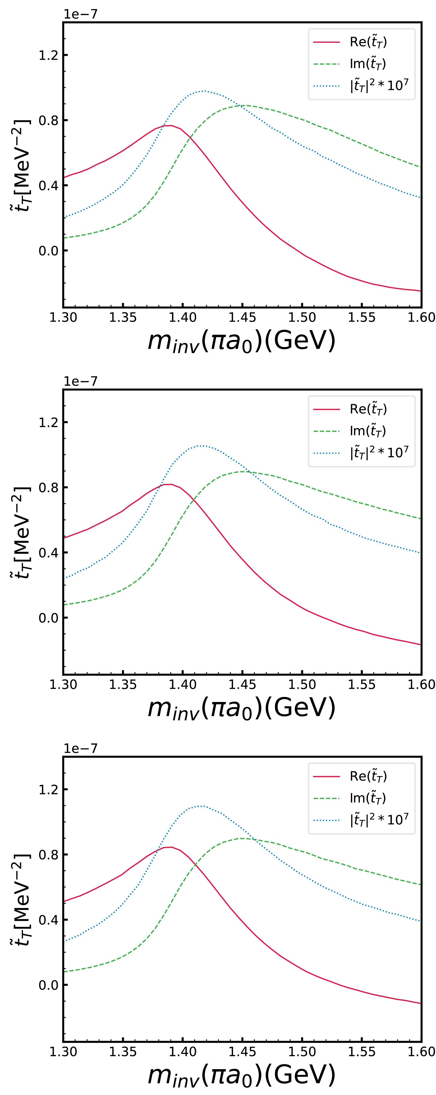
Figure 3. (color online) The
$ \bar{K}^{*0} K^+ K^- $ triangle amplitudes$ \tilde{t}_T $ for$ q_{\text{max}}=600,800, 1000 $ MeV are shown from top to bottom, respectively. We set$ m_{a_0}=980 $ MeV, and$ t_T^2 $ is multiplied by$ 10^{7} $ .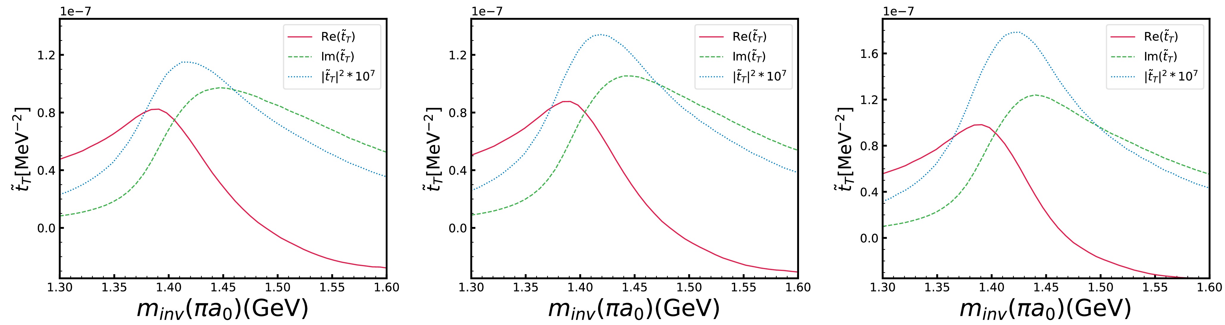
Figure 4. (color online) As in Fig. 3, the triangle amplitudes for
$ m_{a_0}=983 $ ,$ 985 $ , and$ 987 $ MeV with$ q_{\text{max}}=600 $ MeV are shown.Following Ref. [53], Fig. 5 illustrates the development of the TS by fixing
$ \Gamma_{K^*}/2 = \epsilon $ at different finite values close to zero. The formation of the TS in the$ \bar{K}^{*0} $ -K-K triangle loop requires the$ a_0(980) $ mass to be slightly above the$ K^- K^+ $ threshold; therefore, we take$ m_{a_0} = 990\; \mathrm{MeV} $ . The distinct origins of the peaks in$ \mathrm{Re}(\tilde{t}_T) $ and$ \mathrm{Im}(\tilde{t}_T) $ indicate that these two components exhibit different behaviors, as shown in the upper and lower panels of Fig. 5. Specifically,$ \mathrm{Re}(\tilde{t}_T) $ exhibits a cusp at the$ \bar{K}^{*0} K $ threshold around$ 1390\; \mathrm{MeV} $ , followed by a sharp decrease near the TS at$ 1420\; \mathrm{MeV} $ . In contrast,$ \mathrm{Im}(\tilde{t}_T) $ develops a narrow peak at$ 1420\; \mathrm{MeV} $ , directly reflecting the emergence of the triangle singularity. Fig. 5 also shows that, as ϵ decreases, the decrease in$ \mathrm{Re}(\tilde{t}_T) $ near$ 1420\; \mathrm{MeV} $ becomes steeper, the cusp near$ 1390\; \mathrm{MeV} $ becomes more pronounced, and the peak in$ \mathrm{Im}(\tilde{t}_T) $ becomes increasingly sharp. In the limit$ \Gamma_{K^*}/2 = \epsilon = 0 $ , the peak of$ \mathrm{Im}(\tilde{t}_T) $ develops into a genuine singularity.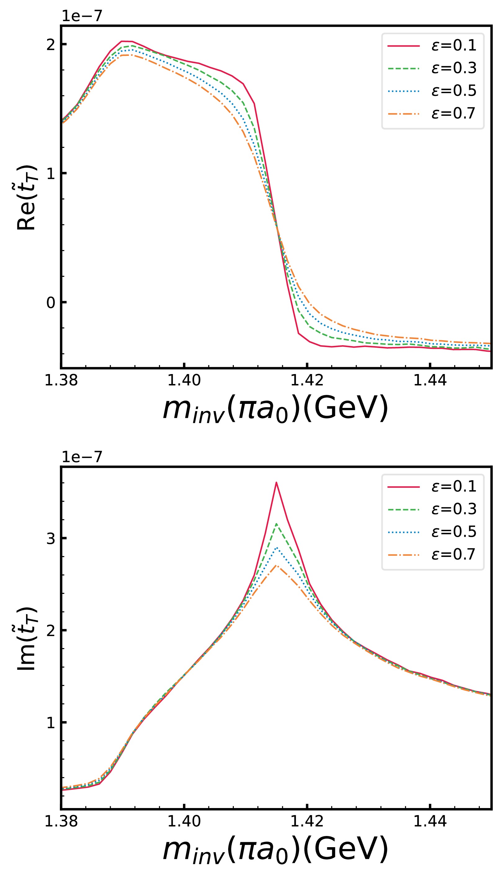
Figure 5. (color online) The dependence of the triangle amplitude Re
$ (\tilde{t}_T) $ and Im$ (\tilde{t}_T) $ on the widths of the internal particles is shown in the upper and lower panels, respectively. We set$ m_{a_0}=990 $ MeV, which is slightly larger than the$ K^- K^+ $ threshold, and use$ \Gamma_{\bar{K}^{*0}}/2=\epsilon=0.1,\ 0.3,\ 0.5 $ , and 0.7 MeV.In Fig. 6, the differential distributions
$\dfrac{{\rm d} \Gamma^\prime}{{\rm d} m_{\text{inv}(\pi a_0)}}$ , Eq. (24), and$\dfrac{1}{\Gamma_{B^0}}\dfrac{{\rm d}^2 \Gamma^\prime}{{\rm d} m_{\text{inv}}(\pi a_0) {\rm d} m_{\text{inv}}(\pi \eta)}$ , Eq. (36), are shown as functions of the invariant masses$ m_{\text{inv}}(\pi a_0) $ and$ m_{\rm{inv}}(\pi \eta) $ in the upper and lower panels, respectively. In the upper panel of Fig. 6, the differential mass distribution for the$ B^0 \to D^- \pi^+ a_0(980) $ decay with respect to$ m_{\rm{inv}}(\pi a_0) $ is shown for fixed values$ m_{\rm{inv}}(\pi \eta) = 980,985,987 $ and$ 988\; \mathrm{MeV} $ with$ q_{\rm{max}} = 600\; \mathrm{MeV} $ . It is evident that increasing$ m_{a_0} $ enhances the decay width of$ B^0 $ , while the peak position remains at the TS,$ m_{\rm{inv}}(\pi a_0) \simeq 1420\; \mathrm{MeV} $ . In the lower panel of Fig. 6, the dependence of$\dfrac{1}{\Gamma_{B^0}}\dfrac{{\rm d}^2 \Gamma^\prime}{{\rm d} m_{\text{inv}}(\pi a_0){\rm d} m_{\text{inv}}(\pi \eta)}$ on$ m_{\rm{inv}}(\pi \eta) $ is shown for fixed values$ m_{\rm{inv}}(\pi a_0) = 1400, 1410, 1420 $ and$ 1440\; \mathrm{MeV} $ around the TS. A pronounced peak appears around$ 980\; \mathrm{MeV} $ , indicating that the main contribution to the decay width comes from the region$ m_{\rm{inv}}(\pi \eta) \simeq 980\; \mathrm{MeV} $ . Moreover, the peak for$ m_{\rm{inv}}(\pi a_0) = 1420\; \mathrm{MeV} $ , close to the TS, is significantly sharper than those at the other values. Therefore, when focusing on the$ a_0(980) $ region, we can integrate the double differential distribution$\dfrac{1}{\Gamma_B} \dfrac{{\rm d}^2 \Gamma^\prime}{{\rm d} m_{\rm{inv}}(\pi a_0)\, {\rm d} m_{\rm{inv}}(\pi \eta)}$ over$ m_{\rm{inv}}(\pi \eta) $ around$ m_{\rm{inv}}(\pi \eta) = 980\; \mathrm{MeV} $ . In Fig. 7, we present the results obtained by integrating over$ m_{\mathrm{inv}}(\pi\eta) \in [980\; \mathrm{MeV} - \Delta_m,\; 980\; \mathrm{MeV} + \Delta_m] $ with$ \Delta_m = 30,\, 50,\,100 $ and$ 150\; \mathrm{MeV} $ . The results show a clear peak at$ 1420\; \mathrm{MeV} $ when the$ a_0(980) $ is considered a dynamically generated state, consistent with the results in Fig. 6. A comparison of the subfigures for$ q_{\rm{max}} = 600,800 $ and$ 1000\; \mathrm{MeV} $ shows that the decay width exhibits a slight enhancement as the cutoff parameter increases.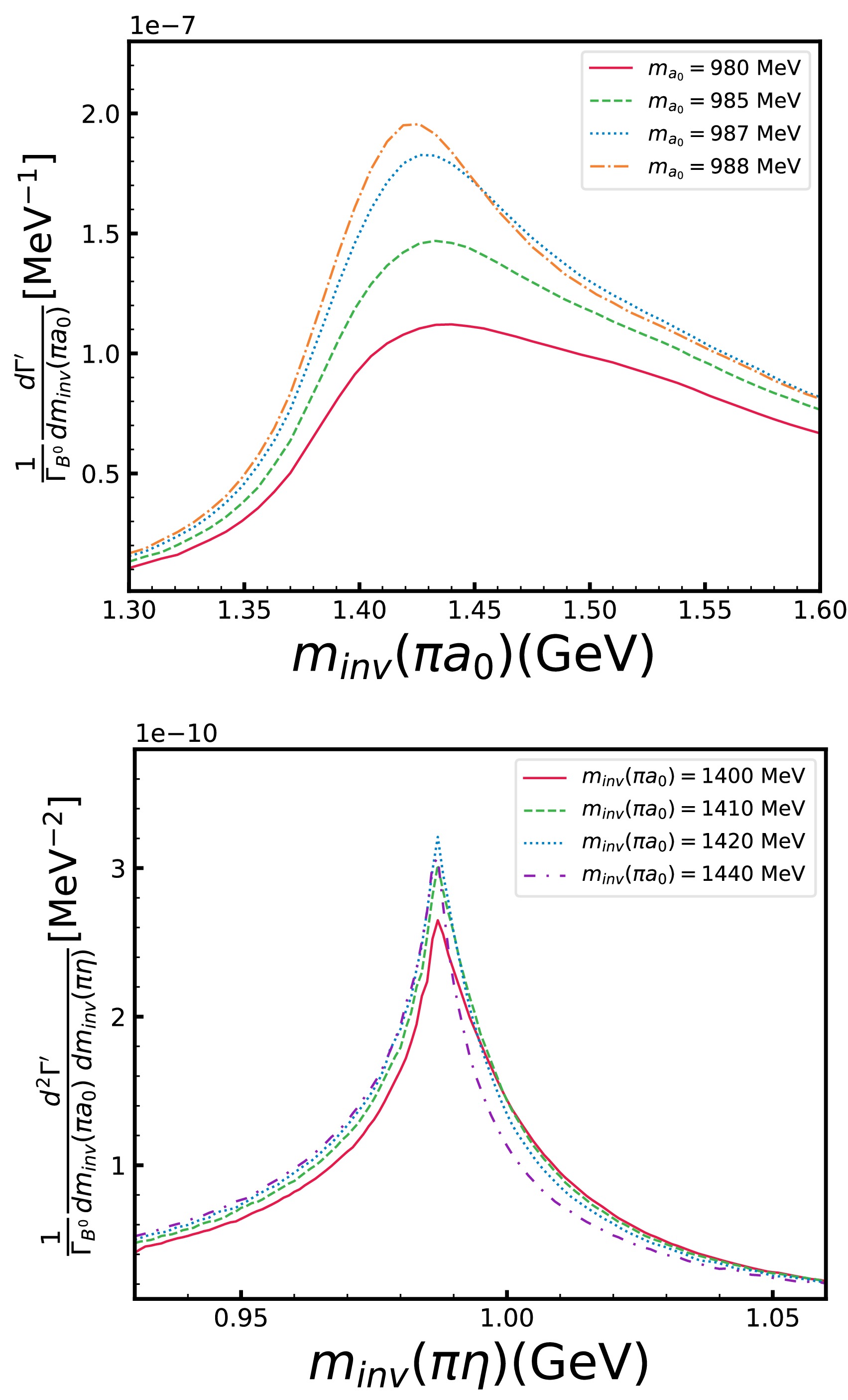
Figure 6. (color online) The upper and lower panels show, respectively, the differential distribution
$\dfrac{{\rm d} \Gamma^\prime}{{\rm d} m_{\text{inv}(\pi a_0)}}$ (Eq. 24) as a function of the invariant mass$ m_{\text{inv}}(\pi a_0) $ and the double differential distribution$\dfrac{1}{\Gamma_{B^0}}\dfrac{{\rm d}^2 \Gamma^\prime}{{\rm d} m_{\text{inv}}(\pi a_0) {\rm d} m_{\text{inv}}(\pi \eta)}$ (Eq. 36) as a function of the invariant masses$ m_{\text{inv}}(\pi a_0) $ and$ m_{\rm{inv}}(\pi \eta) $ .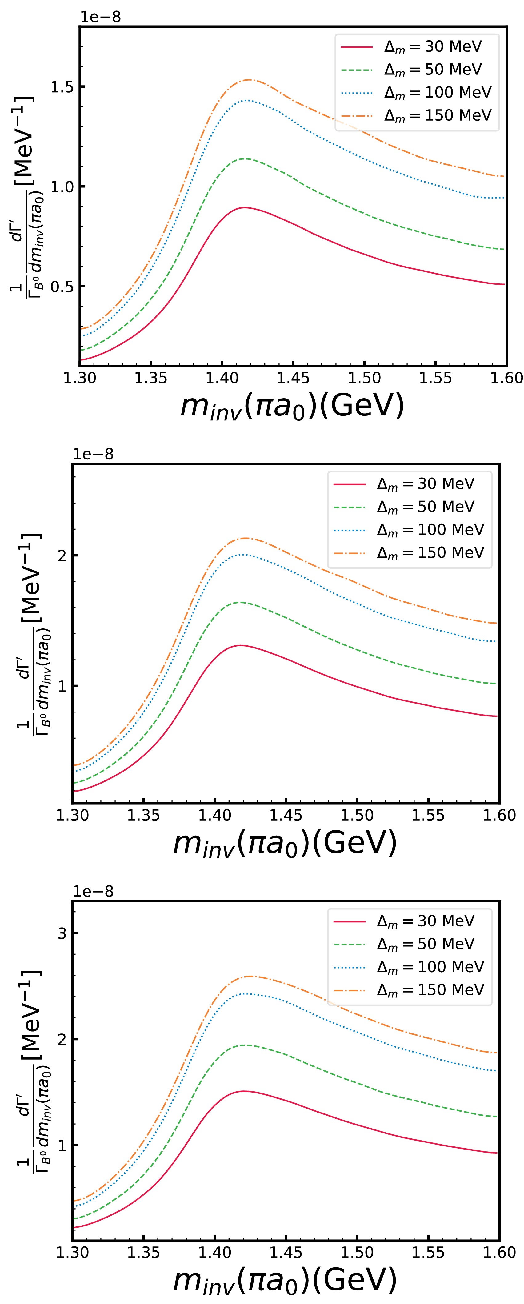
Figure 7. (color online) The differential decay width
$\dfrac{1}{\Gamma_{B^0}}\dfrac{{\rm d}^2 \Gamma^\prime}{{\rm d} m_{\text{inv}}(\pi a_0) {\rm d} m_{\text{inv}}(\pi \eta)}$ is shown as a function of the invariant mass$ m_{\rm{inv}}(\pi a_0) $ , integrated over$ m_{\mathrm{inv}}(\pi\eta) \in [980\; \mathrm{MeV} - $ $ \Delta_m,\; 980\; \mathrm{MeV} + \Delta_m] $ . From top to bottom, the curves correspond to$ q_{\mathrm{max}} = 600,800 $ and$ 1000\; \mathrm{MeV} $ , respectively. -
In Fig. 3, we first present the triangle amplitudes
$ \tilde{t}_T $ ,$ \mathrm{Im}(\tilde{t}_T) $ ,$ \mathrm{Re}(\tilde{t}_T) $ , and$ |\tilde{t}_T|^2 \times 10^{7} $ as functions of the invariant mass$ m_{\rm{inv}}(\pi a_0) $ , with the$ a_0(980) $ mass fixed at$ m_{a_0} = 980\; \mathrm{MeV} $ . The results for$ |\tilde{t}_T|^2 $ exhibit a clear peak around$ 1420\; \mathrm{MeV} $ , consistent with the condition in Eq. (1). The peaks of$ \mathrm{Im}(\tilde{t}_T) $ and$ \mathrm{Re}(\tilde{t}_T) $ appear at$ 1440\; \mathrm{MeV} $ and$ 1390\; \mathrm{MeV} $ , respectively, arising from the TS and the$ \bar{K}^{*0} K^+ $ threshold. From top to bottom, the results correspond to the cutoff parameters$ q_{\rm{max}} = 600, \; 800 $ and$ 1000\; \mathrm{MeV} $ , respectively. As$ q_{\rm{max}} $ increases, the peak positions in$ \mathrm{Im}(\tilde{t}_T) $ ,$ \mathrm{Re}(\tilde{t}_T) $ , and$ |\tilde{t}_T|^2 $ remain unchanged, while their magnitudes generally increase. The triangle amplitudes for different masses of$ a_0(980) $ are shown in Fig. 4. The results indicate that the peaks remain near$ 1420\; \mathrm{MeV} $ , while the strength of the triangle amplitude increases as$ m_{a_0} $ increases. Next, we examine the behavior of the triangle amplitudes$ \mathrm{Im}(\tilde{t}_T) $ and$ \mathrm{Re}(\tilde{t}_T) $ as functions of the internal particle width.
Figure 3. (color online) The
$ \bar{K}^{*0} K^+ K^- $ triangle amplitudes$ \tilde{t}_T $ for$ q_{\text{max}}=600,800, 1000 $ MeV are shown from top to bottom, respectively. We set$ m_{a_0}=980 $ MeV, and$ t_T^2 $ is multiplied by$ 10^{7} $ .
Figure 4. (color online) As in Fig. 3, the triangle amplitudes for
$ m_{a_0}=983 $ ,$ 985 $ , and$ 987 $ MeV with$ q_{\text{max}}=600 $ MeV are shown.Following Ref. [53], Fig. 5 illustrates the development of the TS by fixing
$ \Gamma_{K^*}/2 = \epsilon $ at different finite values close to zero. The formation of the TS in the$ \bar{K}^{*0} $ -K-K triangle loop requires the$ a_0(980) $ mass to be slightly above the$ K^- K^+ $ threshold; therefore, we take$ m_{a_0} = 990\; \mathrm{MeV} $ . The distinct origins of the peaks in$ \mathrm{Re}(\tilde{t}_T) $ and$ \mathrm{Im}(\tilde{t}_T) $ indicate that these two components exhibit different behaviors, as shown in the upper and lower panels of Fig. 5. Specifically,$ \mathrm{Re}(\tilde{t}_T) $ exhibits a cusp at the$ \bar{K}^{*0} K $ threshold around$ 1390\; \mathrm{MeV} $ , followed by a sharp decrease near the TS at$ 1420\; \mathrm{MeV} $ . In contrast,$ \mathrm{Im}(\tilde{t}_T) $ develops a narrow peak at$ 1420\; \mathrm{MeV} $ , directly reflecting the emergence of the triangle singularity. Fig. 5 also shows that, as ϵ decreases, the decrease in$ \mathrm{Re}(\tilde{t}_T) $ near$ 1420\; \mathrm{MeV} $ becomes steeper, the cusp near$ 1390\; \mathrm{MeV} $ becomes more pronounced, and the peak in$ \mathrm{Im}(\tilde{t}_T) $ becomes increasingly sharp. In the limit$ \Gamma_{K^*}/2 = \epsilon = 0 $ , the peak of$ \mathrm{Im}(\tilde{t}_T) $ develops into a genuine singularity.
Figure 5. (color online) The dependence of the triangle amplitude Re
$ (\tilde{t}_T) $ and Im$ (\tilde{t}_T) $ on the widths of the internal particles is shown in the upper and lower panels, respectively. We set$ m_{a_0}=990 $ MeV, which is slightly larger than the$ K^- K^+ $ threshold, and use$ \Gamma_{\bar{K}^{*0}}/2=\epsilon=0.1,\ 0.3,\ 0.5 $ , and 0.7 MeV.In Fig. 6, the differential distributions
$\dfrac{{\rm d} \Gamma^\prime}{{\rm d} m_{\text{inv}(\pi a_0)}}$ , Eq. (24), and$\dfrac{1}{\Gamma_{B^0}}\dfrac{{\rm d}^2 \Gamma^\prime}{{\rm d} m_{\text{inv}}(\pi a_0) {\rm d} m_{\text{inv}}(\pi \eta)}$ , Eq. (36), are shown as functions of the invariant masses$ m_{\text{inv}}(\pi a_0) $ and$ m_{\rm{inv}}(\pi \eta) $ in the upper and lower panels, respectively. In the upper panel of Fig. 6, the differential mass distribution for the$ B^0 \to D^- \pi^+ a_0(980) $ decay with respect to$ m_{\rm{inv}}(\pi a_0) $ is shown for fixed values$ m_{\rm{inv}}(\pi \eta) = 980,985,987 $ and$ 988\; \mathrm{MeV} $ with$ q_{\rm{max}} = 600\; \mathrm{MeV} $ . It is evident that increasing$ m_{a_0} $ enhances the decay width of$ B^0 $ , while the peak position remains at the TS,$ m_{\rm{inv}}(\pi a_0) \simeq 1420\; \mathrm{MeV} $ . In the lower panel of Fig. 6, the dependence of$\dfrac{1}{\Gamma_{B^0}}\dfrac{{\rm d}^2 \Gamma^\prime}{{\rm d} m_{\text{inv}}(\pi a_0){\rm d} m_{\text{inv}}(\pi \eta)}$ on$ m_{\rm{inv}}(\pi \eta) $ is shown for fixed values$ m_{\rm{inv}}(\pi a_0) = 1400, 1410, 1420 $ and$ 1440\; \mathrm{MeV} $ around the TS. A pronounced peak appears around$ 980\; \mathrm{MeV} $ , indicating that the main contribution to the decay width comes from the region$ m_{\rm{inv}}(\pi \eta) \simeq 980\; \mathrm{MeV} $ . Moreover, the peak for$ m_{\rm{inv}}(\pi a_0) = 1420\; \mathrm{MeV} $ , close to the TS, is significantly sharper than those at the other values. Therefore, when focusing on the$ a_0(980) $ region, we can integrate the double differential distribution$\dfrac{1}{\Gamma_B} \dfrac{{\rm d}^2 \Gamma^\prime}{{\rm d} m_{\rm{inv}}(\pi a_0)\, {\rm d} m_{\rm{inv}}(\pi \eta)}$ over$ m_{\rm{inv}}(\pi \eta) $ around$ m_{\rm{inv}}(\pi \eta) = 980\; \mathrm{MeV} $ . In Fig. 7, we present the results obtained by integrating over$ m_{\mathrm{inv}}(\pi\eta) \in [980\; \mathrm{MeV} - \Delta_m,\; 980\; \mathrm{MeV} + \Delta_m] $ with$ \Delta_m = 30,\, 50,\,100 $ and$ 150\; \mathrm{MeV} $ . The results show a clear peak at$ 1420\; \mathrm{MeV} $ when the$ a_0(980) $ is considered a dynamically generated state, consistent with the results in Fig. 6. A comparison of the subfigures for$ q_{\rm{max}} = 600,800 $ and$ 1000\; \mathrm{MeV} $ shows that the decay width exhibits a slight enhancement as the cutoff parameter increases.
Figure 6. (color online) The upper and lower panels show, respectively, the differential distribution
$\dfrac{{\rm d} \Gamma^\prime}{{\rm d} m_{\text{inv}(\pi a_0)}}$ (Eq. 24) as a function of the invariant mass$ m_{\text{inv}}(\pi a_0) $ and the double differential distribution$\dfrac{1}{\Gamma_{B^0}}\dfrac{{\rm d}^2 \Gamma^\prime}{{\rm d} m_{\text{inv}}(\pi a_0) {\rm d} m_{\text{inv}}(\pi \eta)}$ (Eq. 36) as a function of the invariant masses$ m_{\text{inv}}(\pi a_0) $ and$ m_{\rm{inv}}(\pi \eta) $ .
Figure 7. (color online) The differential decay width
$\dfrac{1}{\Gamma_{B^0}}\dfrac{{\rm d}^2 \Gamma^\prime}{{\rm d} m_{\text{inv}}(\pi a_0) {\rm d} m_{\text{inv}}(\pi \eta)}$ is shown as a function of the invariant mass$ m_{\rm{inv}}(\pi a_0) $ , integrated over$ m_{\mathrm{inv}}(\pi\eta) \in [980\; \mathrm{MeV} - $ $ \Delta_m,\; 980\; \mathrm{MeV} + \Delta_m] $ . From top to bottom, the curves correspond to$ q_{\mathrm{max}} = 600,800 $ and$ 1000\; \mathrm{MeV} $ , respectively. -
In Fig. 3, we first present the triangle amplitudes
$ \tilde{t}_T $ ,$ \mathrm{Im}(\tilde{t}_T) $ ,$ \mathrm{Re}(\tilde{t}_T) $ , and$ |\tilde{t}_T|^2 \times 10^{7} $ as functions of the invariant mass$ m_{\rm{inv}}(\pi a_0) $ , with the$ a_0(980) $ mass fixed at$ m_{a_0} = 980\; \mathrm{MeV} $ . The results for$ |\tilde{t}_T|^2 $ exhibit a clear peak around$ 1420\; \mathrm{MeV} $ , consistent with the condition in Eq. (1). The peaks of$ \mathrm{Im}(\tilde{t}_T) $ and$ \mathrm{Re}(\tilde{t}_T) $ appear at$ 1440\; \mathrm{MeV} $ and$ 1390\; \mathrm{MeV} $ , respectively, arising from the TS and the$ \bar{K}^{*0} K^+ $ threshold. From top to bottom, the results correspond to the cutoff parameters$ q_{\rm{max}} = 600, \; 800 $ and$ 1000\; \mathrm{MeV} $ , respectively. As$ q_{\rm{max}} $ increases, the peak positions in$ \mathrm{Im}(\tilde{t}_T) $ ,$ \mathrm{Re}(\tilde{t}_T) $ , and$ |\tilde{t}_T|^2 $ remain unchanged, while their magnitudes generally increase. The triangle amplitudes for different masses of$ a_0(980) $ are shown in Fig. 4. The results indicate that the peaks remain near$ 1420\; \mathrm{MeV} $ , while the strength of the triangle amplitude increases as$ m_{a_0} $ increases. Next, we examine the behavior of the triangle amplitudes$ \mathrm{Im}(\tilde{t}_T) $ and$ \mathrm{Re}(\tilde{t}_T) $ as functions of the internal particle width.
Figure 3. (color online) The
$ \bar{K}^{*0} K^+ K^- $ triangle amplitudes$ \tilde{t}_T $ for$ q_{\text{max}}=600,800, 1000 $ MeV are shown from top to bottom, respectively. We set$ m_{a_0}=980 $ MeV, and$ t_T^2 $ is multiplied by$ 10^{7} $ .
Figure 4. (color online) As in Fig. 3, the triangle amplitudes for
$ m_{a_0}=983 $ ,$ 985 $ , and$ 987 $ MeV with$ q_{\text{max}}=600 $ MeV are shown.Following Ref. [53], Fig. 5 illustrates the development of the TS by fixing
$ \Gamma_{K^*}/2 = \epsilon $ at different finite values close to zero. The formation of the TS in the$ \bar{K}^{*0} $ -K-K triangle loop requires the$ a_0(980) $ mass to be slightly above the$ K^- K^+ $ threshold; therefore, we take$ m_{a_0} = 990\; \mathrm{MeV} $ . The distinct origins of the peaks in$ \mathrm{Re}(\tilde{t}_T) $ and$ \mathrm{Im}(\tilde{t}_T) $ indicate that these two components exhibit different behaviors, as shown in the upper and lower panels of Fig. 5. Specifically,$ \mathrm{Re}(\tilde{t}_T) $ exhibits a cusp at the$ \bar{K}^{*0} K $ threshold around$ 1390\; \mathrm{MeV} $ , followed by a sharp decrease near the TS at$ 1420\; \mathrm{MeV} $ . In contrast,$ \mathrm{Im}(\tilde{t}_T) $ develops a narrow peak at$ 1420\; \mathrm{MeV} $ , directly reflecting the emergence of the triangle singularity. Fig. 5 also shows that, as ϵ decreases, the decrease in$ \mathrm{Re}(\tilde{t}_T) $ near$ 1420\; \mathrm{MeV} $ becomes steeper, the cusp near$ 1390\; \mathrm{MeV} $ becomes more pronounced, and the peak in$ \mathrm{Im}(\tilde{t}_T) $ becomes increasingly sharp. In the limit$ \Gamma_{K^*}/2 = \epsilon = 0 $ , the peak of$ \mathrm{Im}(\tilde{t}_T) $ develops into a genuine singularity.
Figure 5. (color online) The dependence of the triangle amplitude Re
$ (\tilde{t}_T) $ and Im$ (\tilde{t}_T) $ on the widths of the internal particles is shown in the upper and lower panels, respectively. We set$ m_{a_0}=990 $ MeV, which is slightly larger than the$ K^- K^+ $ threshold, and use$ \Gamma_{\bar{K}^{*0}}/2=\epsilon=0.1,\ 0.3,\ 0.5 $ , and 0.7 MeV.In Fig. 6, the differential distributions
$\dfrac{{\rm d} \Gamma^\prime}{{\rm d} m_{\text{inv}(\pi a_0)}}$ , Eq. (24), and$\dfrac{1}{\Gamma_{B^0}}\dfrac{{\rm d}^2 \Gamma^\prime}{{\rm d} m_{\text{inv}}(\pi a_0) {\rm d} m_{\text{inv}}(\pi \eta)}$ , Eq. (36), are shown as functions of the invariant masses$ m_{\text{inv}}(\pi a_0) $ and$ m_{\rm{inv}}(\pi \eta) $ in the upper and lower panels, respectively. In the upper panel of Fig. 6, the differential mass distribution for the$ B^0 \to D^- \pi^+ a_0(980) $ decay with respect to$ m_{\rm{inv}}(\pi a_0) $ is shown for fixed values$ m_{\rm{inv}}(\pi \eta) = 980,985,987 $ and$ 988\; \mathrm{MeV} $ with$ q_{\rm{max}} = 600\; \mathrm{MeV} $ . It is evident that increasing$ m_{a_0} $ enhances the decay width of$ B^0 $ , while the peak position remains at the TS,$ m_{\rm{inv}}(\pi a_0) \simeq 1420\; \mathrm{MeV} $ . In the lower panel of Fig. 6, the dependence of$\dfrac{1}{\Gamma_{B^0}}\dfrac{{\rm d}^2 \Gamma^\prime}{{\rm d} m_{\text{inv}}(\pi a_0){\rm d} m_{\text{inv}}(\pi \eta)}$ on$ m_{\rm{inv}}(\pi \eta) $ is shown for fixed values$ m_{\rm{inv}}(\pi a_0) = 1400, 1410, 1420 $ and$ 1440\; \mathrm{MeV} $ around the TS. A pronounced peak appears around$ 980\; \mathrm{MeV} $ , indicating that the main contribution to the decay width comes from the region$ m_{\rm{inv}}(\pi \eta) \simeq 980\; \mathrm{MeV} $ . Moreover, the peak for$ m_{\rm{inv}}(\pi a_0) = 1420\; \mathrm{MeV} $ , close to the TS, is significantly sharper than those at the other values. Therefore, when focusing on the$ a_0(980) $ region, we can integrate the double differential distribution$\dfrac{1}{\Gamma_B} \dfrac{{\rm d}^2 \Gamma^\prime}{{\rm d} m_{\rm{inv}}(\pi a_0)\, {\rm d} m_{\rm{inv}}(\pi \eta)}$ over$ m_{\rm{inv}}(\pi \eta) $ around$ m_{\rm{inv}}(\pi \eta) = 980\; \mathrm{MeV} $ . In Fig. 7, we present the results obtained by integrating over$ m_{\mathrm{inv}}(\pi\eta) \in [980\; \mathrm{MeV} - \Delta_m,\; 980\; \mathrm{MeV} + \Delta_m] $ with$ \Delta_m = 30,\, 50,\,100 $ and$ 150\; \mathrm{MeV} $ . The results show a clear peak at$ 1420\; \mathrm{MeV} $ when the$ a_0(980) $ is considered a dynamically generated state, consistent with the results in Fig. 6. A comparison of the subfigures for$ q_{\rm{max}} = 600,800 $ and$ 1000\; \mathrm{MeV} $ shows that the decay width exhibits a slight enhancement as the cutoff parameter increases.
Figure 6. (color online) The upper and lower panels show, respectively, the differential distribution
$\dfrac{{\rm d} \Gamma^\prime}{{\rm d} m_{\text{inv}(\pi a_0)}}$ (Eq. 24) as a function of the invariant mass$ m_{\text{inv}}(\pi a_0) $ and the double differential distribution$\dfrac{1}{\Gamma_{B^0}}\dfrac{{\rm d}^2 \Gamma^\prime}{{\rm d} m_{\text{inv}}(\pi a_0) {\rm d} m_{\text{inv}}(\pi \eta)}$ (Eq. 36) as a function of the invariant masses$ m_{\text{inv}}(\pi a_0) $ and$ m_{\rm{inv}}(\pi \eta) $ .
Figure 7. (color online) The differential decay width
$\dfrac{1}{\Gamma_{B^0}}\dfrac{{\rm d}^2 \Gamma^\prime}{{\rm d} m_{\text{inv}}(\pi a_0) {\rm d} m_{\text{inv}}(\pi \eta)}$ is shown as a function of the invariant mass$ m_{\rm{inv}}(\pi a_0) $ , integrated over$ m_{\mathrm{inv}}(\pi\eta) \in [980\; \mathrm{MeV} - $ $ \Delta_m,\; 980\; \mathrm{MeV} + \Delta_m] $ . From top to bottom, the curves correspond to$ q_{\mathrm{max}} = 600,800 $ and$ 1000\; \mathrm{MeV} $ , respectively. -
In Fig. 3, we first present the triangle amplitudes
$ \tilde{t}_T $ ,$ \mathrm{Im}(\tilde{t}_T) $ ,$ \mathrm{Re}(\tilde{t}_T) $ , and$ |\tilde{t}_T|^2 \times 10^{7} $ as functions of the invariant mass$ m_{\rm{inv}}(\pi a_0) $ , with the$ a_0(980) $ mass fixed at$ m_{a_0} = 980\; \mathrm{MeV} $ . The results for$ |\tilde{t}_T|^2 $ exhibit a clear peak around$ 1420\; \mathrm{MeV} $ , consistent with the condition in Eq. (1). The peaks of$ \mathrm{Im}(\tilde{t}_T) $ and$ \mathrm{Re}(\tilde{t}_T) $ appear at$ 1440\; \mathrm{MeV} $ and$ 1390\; \mathrm{MeV} $ , respectively, arising from the TS and the$ \bar{K}^{*0} K^+ $ threshold. From top to bottom, the results correspond to the cutoff parameters$ q_{\rm{max}} = 600, \; 800 $ and$ 1000\; \mathrm{MeV} $ , respectively. As$ q_{\rm{max}} $ increases, the peak positions in$ \mathrm{Im}(\tilde{t}_T) $ ,$ \mathrm{Re}(\tilde{t}_T) $ , and$ |\tilde{t}_T|^2 $ remain unchanged, while their magnitudes generally increase. The triangle amplitudes for different masses of$ a_0(980) $ are shown in Fig. 4. The results indicate that the peaks remain near$ 1420\; \mathrm{MeV} $ , while the strength of the triangle amplitude increases as$ m_{a_0} $ increases. Next, we examine the behavior of the triangle amplitudes$ \mathrm{Im}(\tilde{t}_T) $ and$ \mathrm{Re}(\tilde{t}_T) $ as functions of the internal particle width.
Figure 3. (color online) The
$ \bar{K}^{*0} K^+ K^- $ triangle amplitudes$ \tilde{t}_T $ for$ q_{\text{max}}=600,800, 1000 $ MeV are shown from top to bottom, respectively. We set$ m_{a_0}=980 $ MeV, and$ t_T^2 $ is multiplied by$ 10^{7} $ .
Figure 4. (color online) As in Fig. 3, the triangle amplitudes for
$ m_{a_0}=983 $ ,$ 985 $ , and$ 987 $ MeV with$ q_{\text{max}}=600 $ MeV are shown.Following Ref. [53], Fig. 5 illustrates the development of the TS by fixing
$ \Gamma_{K^*}/2 = \epsilon $ at different finite values close to zero. The formation of the TS in the$ \bar{K}^{*0} $ -K-K triangle loop requires the$ a_0(980) $ mass to be slightly above the$ K^- K^+ $ threshold; therefore, we take$ m_{a_0} = 990\; \mathrm{MeV} $ . The distinct origins of the peaks in$ \mathrm{Re}(\tilde{t}_T) $ and$ \mathrm{Im}(\tilde{t}_T) $ indicate that these two components exhibit different behaviors, as shown in the upper and lower panels of Fig. 5. Specifically,$ \mathrm{Re}(\tilde{t}_T) $ exhibits a cusp at the$ \bar{K}^{*0} K $ threshold around$ 1390\; \mathrm{MeV} $ , followed by a sharp decrease near the TS at$ 1420\; \mathrm{MeV} $ . In contrast,$ \mathrm{Im}(\tilde{t}_T) $ develops a narrow peak at$ 1420\; \mathrm{MeV} $ , directly reflecting the emergence of the triangle singularity. Fig. 5 also shows that, as ϵ decreases, the decrease in$ \mathrm{Re}(\tilde{t}_T) $ near$ 1420\; \mathrm{MeV} $ becomes steeper, the cusp near$ 1390\; \mathrm{MeV} $ becomes more pronounced, and the peak in$ \mathrm{Im}(\tilde{t}_T) $ becomes increasingly sharp. In the limit$ \Gamma_{K^*}/2 = \epsilon = 0 $ , the peak of$ \mathrm{Im}(\tilde{t}_T) $ develops into a genuine singularity.
Figure 5. (color online) The dependence of the triangle amplitude Re
$ (\tilde{t}_T) $ and Im$ (\tilde{t}_T) $ on the widths of the internal particles is shown in the upper and lower panels, respectively. We set$ m_{a_0}=990 $ MeV, which is slightly larger than the$ K^- K^+ $ threshold, and use$ \Gamma_{\bar{K}^{*0}}/2=\epsilon=0.1,\ 0.3,\ 0.5 $ , and 0.7 MeV.In Fig. 6, the differential distributions
$\dfrac{{\rm d} \Gamma^\prime}{{\rm d} m_{\text{inv}(\pi a_0)}}$ , Eq. (24), and$\dfrac{1}{\Gamma_{B^0}}\dfrac{{\rm d}^2 \Gamma^\prime}{{\rm d} m_{\text{inv}}(\pi a_0) {\rm d} m_{\text{inv}}(\pi \eta)}$ , Eq. (36), are shown as functions of the invariant masses$ m_{\text{inv}}(\pi a_0) $ and$ m_{\rm{inv}}(\pi \eta) $ in the upper and lower panels, respectively. In the upper panel of Fig. 6, the differential mass distribution for the$ B^0 \to D^- \pi^+ a_0(980) $ decay with respect to$ m_{\rm{inv}}(\pi a_0) $ is shown for fixed values$ m_{\rm{inv}}(\pi \eta) = 980,985,987 $ and$ 988\; \mathrm{MeV} $ with$ q_{\rm{max}} = 600\; \mathrm{MeV} $ . It is evident that increasing$ m_{a_0} $ enhances the decay width of$ B^0 $ , while the peak position remains at the TS,$ m_{\rm{inv}}(\pi a_0) \simeq 1420\; \mathrm{MeV} $ . In the lower panel of Fig. 6, the dependence of$\dfrac{1}{\Gamma_{B^0}}\dfrac{{\rm d}^2 \Gamma^\prime}{{\rm d} m_{\text{inv}}(\pi a_0){\rm d} m_{\text{inv}}(\pi \eta)}$ on$ m_{\rm{inv}}(\pi \eta) $ is shown for fixed values$ m_{\rm{inv}}(\pi a_0) = 1400, 1410, 1420 $ and$ 1440\; \mathrm{MeV} $ around the TS. A pronounced peak appears around$ 980\; \mathrm{MeV} $ , indicating that the main contribution to the decay width comes from the region$ m_{\rm{inv}}(\pi \eta) \simeq 980\; \mathrm{MeV} $ . Moreover, the peak for$ m_{\rm{inv}}(\pi a_0) = 1420\; \mathrm{MeV} $ , close to the TS, is significantly sharper than those at the other values. Therefore, when focusing on the$ a_0(980) $ region, we can integrate the double differential distribution$\dfrac{1}{\Gamma_B} \dfrac{{\rm d}^2 \Gamma^\prime}{{\rm d} m_{\rm{inv}}(\pi a_0)\, {\rm d} m_{\rm{inv}}(\pi \eta)}$ over$ m_{\rm{inv}}(\pi \eta) $ around$ m_{\rm{inv}}(\pi \eta) = 980\; \mathrm{MeV} $ . In Fig. 7, we present the results obtained by integrating over$ m_{\mathrm{inv}}(\pi\eta) \in [980\; \mathrm{MeV} - \Delta_m,\; 980\; \mathrm{MeV} + \Delta_m] $ with$ \Delta_m = 30,\, 50,\,100 $ and$ 150\; \mathrm{MeV} $ . The results show a clear peak at$ 1420\; \mathrm{MeV} $ when the$ a_0(980) $ is considered a dynamically generated state, consistent with the results in Fig. 6. A comparison of the subfigures for$ q_{\rm{max}} = 600,800 $ and$ 1000\; \mathrm{MeV} $ shows that the decay width exhibits a slight enhancement as the cutoff parameter increases.
Figure 6. (color online) The upper and lower panels show, respectively, the differential distribution
$\dfrac{{\rm d} \Gamma^\prime}{{\rm d} m_{\text{inv}(\pi a_0)}}$ (Eq. 24) as a function of the invariant mass$ m_{\text{inv}}(\pi a_0) $ and the double differential distribution$\dfrac{1}{\Gamma_{B^0}}\dfrac{{\rm d}^2 \Gamma^\prime}{{\rm d} m_{\text{inv}}(\pi a_0) {\rm d} m_{\text{inv}}(\pi \eta)}$ (Eq. 36) as a function of the invariant masses$ m_{\text{inv}}(\pi a_0) $ and$ m_{\rm{inv}}(\pi \eta) $ .
Figure 7. (color online) The differential decay width
$\dfrac{1}{\Gamma_{B^0}}\dfrac{{\rm d}^2 \Gamma^\prime}{{\rm d} m_{\text{inv}}(\pi a_0) {\rm d} m_{\text{inv}}(\pi \eta)}$ is shown as a function of the invariant mass$ m_{\rm{inv}}(\pi a_0) $ , integrated over$ m_{\mathrm{inv}}(\pi\eta) \in [980\; \mathrm{MeV} - $ $ \Delta_m,\; 980\; \mathrm{MeV} + \Delta_m] $ . From top to bottom, the curves correspond to$ q_{\mathrm{max}} = 600,800 $ and$ 1000\; \mathrm{MeV} $ , respectively. -
In Fig. 3, we first present the triangle amplitudes
$ \tilde{t}_T $ ,$ \mathrm{Im}(\tilde{t}_T) $ ,$ \mathrm{Re}(\tilde{t}_T) $ , and$ |\tilde{t}_T|^2 \times 10^{7} $ as functions of the invariant mass$ m_{\rm{inv}}(\pi a_0) $ , with the$ a_0(980) $ mass fixed at$ m_{a_0} = 980\; \mathrm{MeV} $ . The results for$ |\tilde{t}_T|^2 $ exhibit a clear peak around$ 1420\; \mathrm{MeV} $ , consistent with the condition in Eq. (1). The peaks of$ \mathrm{Im}(\tilde{t}_T) $ and$ \mathrm{Re}(\tilde{t}_T) $ appear at$ 1440\; \mathrm{MeV} $ and$ 1390\; \mathrm{MeV} $ , respectively, arising from the TS and the$ \bar{K}^{*0} K^+ $ threshold. From top to bottom, the results correspond to the cutoff parameters$ q_{\rm{max}} = 600, \; 800 $ and$ 1000\; \mathrm{MeV} $ , respectively. As$ q_{\rm{max}} $ increases, the peak positions in$ \mathrm{Im}(\tilde{t}_T) $ ,$ \mathrm{Re}(\tilde{t}_T) $ , and$ |\tilde{t}_T|^2 $ remain unchanged, while their magnitudes generally increase. The triangle amplitudes for different masses of$ a_0(980) $ are shown in Fig. 4. The results indicate that the peaks remain near$ 1420\; \mathrm{MeV} $ , while the strength of the triangle amplitude increases as$ m_{a_0} $ increases. Next, we examine the behavior of the triangle amplitudes$ \mathrm{Im}(\tilde{t}_T) $ and$ \mathrm{Re}(\tilde{t}_T) $ as functions of the internal particle width.
Figure 3. (color online) The
$ \bar{K}^{*0} K^+ K^- $ triangle amplitudes$ \tilde{t}_T $ for$ q_{\text{max}}=600,800, 1000 $ MeV are shown from top to bottom, respectively. We set$ m_{a_0}=980 $ MeV, and$ t_T^2 $ is multiplied by$ 10^{7} $ .
Figure 4. (color online) As in Fig. 3, the triangle amplitudes for
$ m_{a_0}=983 $ ,$ 985 $ , and$ 987 $ MeV with$ q_{\text{max}}=600 $ MeV are shown.Following Ref. [53], Fig. 5 illustrates the development of the TS by fixing
$ \Gamma_{K^*}/2 = \epsilon $ at different finite values close to zero. The formation of the TS in the$ \bar{K}^{*0} $ -K-K triangle loop requires the$ a_0(980) $ mass to be slightly above the$ K^- K^+ $ threshold; therefore, we take$ m_{a_0} = 990\; \mathrm{MeV} $ . The distinct origins of the peaks in$ \mathrm{Re}(\tilde{t}_T) $ and$ \mathrm{Im}(\tilde{t}_T) $ indicate that these two components exhibit different behaviors, as shown in the upper and lower panels of Fig. 5. Specifically,$ \mathrm{Re}(\tilde{t}_T) $ exhibits a cusp at the$ \bar{K}^{*0} K $ threshold around$ 1390\; \mathrm{MeV} $ , followed by a sharp decrease near the TS at$ 1420\; \mathrm{MeV} $ . In contrast,$ \mathrm{Im}(\tilde{t}_T) $ develops a narrow peak at$ 1420\; \mathrm{MeV} $ , directly reflecting the emergence of the triangle singularity. Fig. 5 also shows that, as ϵ decreases, the decrease in$ \mathrm{Re}(\tilde{t}_T) $ near$ 1420\; \mathrm{MeV} $ becomes steeper, the cusp near$ 1390\; \mathrm{MeV} $ becomes more pronounced, and the peak in$ \mathrm{Im}(\tilde{t}_T) $ becomes increasingly sharp. In the limit$ \Gamma_{K^*}/2 = \epsilon = 0 $ , the peak of$ \mathrm{Im}(\tilde{t}_T) $ develops into a genuine singularity.
Figure 5. (color online) The dependence of the triangle amplitude Re
$ (\tilde{t}_T) $ and Im$ (\tilde{t}_T) $ on the widths of the internal particles is shown in the upper and lower panels, respectively. We set$ m_{a_0}=990 $ MeV, which is slightly larger than the$ K^- K^+ $ threshold, and use$ \Gamma_{\bar{K}^{*0}}/2=\epsilon=0.1,\ 0.3,\ 0.5 $ , and 0.7 MeV.In Fig. 6, the differential distributions
$\dfrac{{\rm d} \Gamma^\prime}{{\rm d} m_{\text{inv}(\pi a_0)}}$ , Eq. (24), and$\dfrac{1}{\Gamma_{B^0}}\dfrac{{\rm d}^2 \Gamma^\prime}{{\rm d} m_{\text{inv}}(\pi a_0) {\rm d} m_{\text{inv}}(\pi \eta)}$ , Eq. (36), are shown as functions of the invariant masses$ m_{\text{inv}}(\pi a_0) $ and$ m_{\rm{inv}}(\pi \eta) $ in the upper and lower panels, respectively. In the upper panel of Fig. 6, the differential mass distribution for the$ B^0 \to D^- \pi^+ a_0(980) $ decay with respect to$ m_{\rm{inv}}(\pi a_0) $ is shown for fixed values$ m_{\rm{inv}}(\pi \eta) = 980,985,987 $ and$ 988\; \mathrm{MeV} $ with$ q_{\rm{max}} = 600\; \mathrm{MeV} $ . It is evident that increasing$ m_{a_0} $ enhances the decay width of$ B^0 $ , while the peak position remains at the TS,$ m_{\rm{inv}}(\pi a_0) \simeq 1420\; \mathrm{MeV} $ . In the lower panel of Fig. 6, the dependence of$\dfrac{1}{\Gamma_{B^0}}\dfrac{{\rm d}^2 \Gamma^\prime}{{\rm d} m_{\text{inv}}(\pi a_0){\rm d} m_{\text{inv}}(\pi \eta)}$ on$ m_{\rm{inv}}(\pi \eta) $ is shown for fixed values$ m_{\rm{inv}}(\pi a_0) = 1400, 1410, 1420 $ and$ 1440\; \mathrm{MeV} $ around the TS. A pronounced peak appears around$ 980\; \mathrm{MeV} $ , indicating that the main contribution to the decay width comes from the region$ m_{\rm{inv}}(\pi \eta) \simeq 980\; \mathrm{MeV} $ . Moreover, the peak for$ m_{\rm{inv}}(\pi a_0) = 1420\; \mathrm{MeV} $ , close to the TS, is significantly sharper than those at the other values. Therefore, when focusing on the$ a_0(980) $ region, we can integrate the double differential distribution$\dfrac{1}{\Gamma_B} \dfrac{{\rm d}^2 \Gamma^\prime}{{\rm d} m_{\rm{inv}}(\pi a_0)\, {\rm d} m_{\rm{inv}}(\pi \eta)}$ over$ m_{\rm{inv}}(\pi \eta) $ around$ m_{\rm{inv}}(\pi \eta) = 980\; \mathrm{MeV} $ . In Fig. 7, we present the results obtained by integrating over$ m_{\mathrm{inv}}(\pi\eta) \in [980\; \mathrm{MeV} - \Delta_m,\; 980\; \mathrm{MeV} + \Delta_m] $ with$ \Delta_m = 30,\, 50,\,100 $ and$ 150\; \mathrm{MeV} $ . The results show a clear peak at$ 1420\; \mathrm{MeV} $ when the$ a_0(980) $ is considered a dynamically generated state, consistent with the results in Fig. 6. A comparison of the subfigures for$ q_{\rm{max}} = 600,800 $ and$ 1000\; \mathrm{MeV} $ shows that the decay width exhibits a slight enhancement as the cutoff parameter increases.
Figure 6. (color online) The upper and lower panels show, respectively, the differential distribution
$\dfrac{{\rm d} \Gamma^\prime}{{\rm d} m_{\text{inv}(\pi a_0)}}$ (Eq. 24) as a function of the invariant mass$ m_{\text{inv}}(\pi a_0) $ and the double differential distribution$\dfrac{1}{\Gamma_{B^0}}\dfrac{{\rm d}^2 \Gamma^\prime}{{\rm d} m_{\text{inv}}(\pi a_0) {\rm d} m_{\text{inv}}(\pi \eta)}$ (Eq. 36) as a function of the invariant masses$ m_{\text{inv}}(\pi a_0) $ and$ m_{\rm{inv}}(\pi \eta) $ .
Figure 7. (color online) The differential decay width
$\dfrac{1}{\Gamma_{B^0}}\dfrac{{\rm d}^2 \Gamma^\prime}{{\rm d} m_{\text{inv}}(\pi a_0) {\rm d} m_{\text{inv}}(\pi \eta)}$ is shown as a function of the invariant mass$ m_{\rm{inv}}(\pi a_0) $ , integrated over$ m_{\mathrm{inv}}(\pi\eta) \in [980\; \mathrm{MeV} - $ $ \Delta_m,\; 980\; \mathrm{MeV} + \Delta_m] $ . From top to bottom, the curves correspond to$ q_{\mathrm{max}} = 600,800 $ and$ 1000\; \mathrm{MeV} $ , respectively. -
In Fig. 3, we first present the triangle amplitudes
$ \tilde{t}_T $ ,$ \mathrm{Im}(\tilde{t}_T) $ ,$ \mathrm{Re}(\tilde{t}_T) $ , and$ |\tilde{t}_T|^2 \times 10^{7} $ as functions of the invariant mass$ m_{\rm{inv}}(\pi a_0) $ , with the$ a_0(980) $ mass fixed at$ m_{a_0} = 980\; \mathrm{MeV} $ . The results for$ |\tilde{t}_T|^2 $ exhibit a clear peak around$ 1420\; \mathrm{MeV} $ , consistent with the condition in Eq. (1). The peaks of$ \mathrm{Im}(\tilde{t}_T) $ and$ \mathrm{Re}(\tilde{t}_T) $ appear at$ 1440\; \mathrm{MeV} $ and$ 1390\; \mathrm{MeV} $ , respectively, arising from the TS and the$ \bar{K}^{*0} K^+ $ threshold. From top to bottom, the results correspond to the cutoff parameters$ q_{\rm{max}} = 600, \; 800 $ and$ 1000\; \mathrm{MeV} $ , respectively. As$ q_{\rm{max}} $ increases, the peak positions in$ \mathrm{Im}(\tilde{t}_T) $ ,$ \mathrm{Re}(\tilde{t}_T) $ , and$ |\tilde{t}_T|^2 $ remain unchanged, while their magnitudes generally increase. The triangle amplitudes for different masses of$ a_0(980) $ are shown in Fig. 4. The results indicate that the peaks remain near$ 1420\; \mathrm{MeV} $ , while the strength of the triangle amplitude increases as$ m_{a_0} $ increases. Next, we examine the behavior of the triangle amplitudes$ \mathrm{Im}(\tilde{t}_T) $ and$ \mathrm{Re}(\tilde{t}_T) $ as functions of the internal particle width.
Figure 3. (color online) The
$ \bar{K}^{*0} K^+ K^- $ triangle amplitudes$ \tilde{t}_T $ for$ q_{\text{max}}=600,800, 1000 $ MeV are shown from top to bottom, respectively. We set$ m_{a_0}=980 $ MeV, and$ t_T^2 $ is multiplied by$ 10^{7} $ .
Figure 4. (color online) As in Fig. 3, the triangle amplitudes for
$ m_{a_0}=983 $ ,$ 985 $ , and$ 987 $ MeV with$ q_{\text{max}}=600 $ MeV are shown.Following Ref. [53], Fig. 5 illustrates the development of the TS by fixing
$ \Gamma_{K^*}/2 = \epsilon $ at different finite values close to zero. The formation of the TS in the$ \bar{K}^{*0} $ -K-K triangle loop requires the$ a_0(980) $ mass to be slightly above the$ K^- K^+ $ threshold; therefore, we take$ m_{a_0} = 990\; \mathrm{MeV} $ . The distinct origins of the peaks in$ \mathrm{Re}(\tilde{t}_T) $ and$ \mathrm{Im}(\tilde{t}_T) $ indicate that these two components exhibit different behaviors, as shown in the upper and lower panels of Fig. 5. Specifically,$ \mathrm{Re}(\tilde{t}_T) $ exhibits a cusp at the$ \bar{K}^{*0} K $ threshold around$ 1390\; \mathrm{MeV} $ , followed by a sharp decrease near the TS at$ 1420\; \mathrm{MeV} $ . In contrast,$ \mathrm{Im}(\tilde{t}_T) $ develops a narrow peak at$ 1420\; \mathrm{MeV} $ , directly reflecting the emergence of the triangle singularity. Fig. 5 also shows that, as ϵ decreases, the decrease in$ \mathrm{Re}(\tilde{t}_T) $ near$ 1420\; \mathrm{MeV} $ becomes steeper, the cusp near$ 1390\; \mathrm{MeV} $ becomes more pronounced, and the peak in$ \mathrm{Im}(\tilde{t}_T) $ becomes increasingly sharp. In the limit$ \Gamma_{K^*}/2 = \epsilon = 0 $ , the peak of$ \mathrm{Im}(\tilde{t}_T) $ develops into a genuine singularity.
Figure 5. (color online) The dependence of the triangle amplitude Re
$ (\tilde{t}_T) $ and Im$ (\tilde{t}_T) $ on the widths of the internal particles is shown in the upper and lower panels, respectively. We set$ m_{a_0}=990 $ MeV, which is slightly larger than the$ K^- K^+ $ threshold, and use$ \Gamma_{\bar{K}^{*0}}/2=\epsilon=0.1,\ 0.3,\ 0.5 $ , and 0.7 MeV.In Fig. 6, the differential distributions
$\dfrac{{\rm d} \Gamma^\prime}{{\rm d} m_{\text{inv}(\pi a_0)}}$ , Eq. (24), and$\dfrac{1}{\Gamma_{B^0}}\dfrac{{\rm d}^2 \Gamma^\prime}{{\rm d} m_{\text{inv}}(\pi a_0) {\rm d} m_{\text{inv}}(\pi \eta)}$ , Eq. (36), are shown as functions of the invariant masses$ m_{\text{inv}}(\pi a_0) $ and$ m_{\rm{inv}}(\pi \eta) $ in the upper and lower panels, respectively. In the upper panel of Fig. 6, the differential mass distribution for the$ B^0 \to D^- \pi^+ a_0(980) $ decay with respect to$ m_{\rm{inv}}(\pi a_0) $ is shown for fixed values$ m_{\rm{inv}}(\pi \eta) = 980,985,987 $ and$ 988\; \mathrm{MeV} $ with$ q_{\rm{max}} = 600\; \mathrm{MeV} $ . It is evident that increasing$ m_{a_0} $ enhances the decay width of$ B^0 $ , while the peak position remains at the TS,$ m_{\rm{inv}}(\pi a_0) \simeq 1420\; \mathrm{MeV} $ . In the lower panel of Fig. 6, the dependence of$\dfrac{1}{\Gamma_{B^0}}\dfrac{{\rm d}^2 \Gamma^\prime}{{\rm d} m_{\text{inv}}(\pi a_0){\rm d} m_{\text{inv}}(\pi \eta)}$ on$ m_{\rm{inv}}(\pi \eta) $ is shown for fixed values$ m_{\rm{inv}}(\pi a_0) = 1400, 1410, 1420 $ and$ 1440\; \mathrm{MeV} $ around the TS. A pronounced peak appears around$ 980\; \mathrm{MeV} $ , indicating that the main contribution to the decay width comes from the region$ m_{\rm{inv}}(\pi \eta) \simeq 980\; \mathrm{MeV} $ . Moreover, the peak for$ m_{\rm{inv}}(\pi a_0) = 1420\; \mathrm{MeV} $ , close to the TS, is significantly sharper than those at the other values. Therefore, when focusing on the$ a_0(980) $ region, we can integrate the double differential distribution$\dfrac{1}{\Gamma_B} \dfrac{{\rm d}^2 \Gamma^\prime}{{\rm d} m_{\rm{inv}}(\pi a_0)\, {\rm d} m_{\rm{inv}}(\pi \eta)}$ over$ m_{\rm{inv}}(\pi \eta) $ around$ m_{\rm{inv}}(\pi \eta) = 980\; \mathrm{MeV} $ . In Fig. 7, we present the results obtained by integrating over$ m_{\mathrm{inv}}(\pi\eta) \in [980\; \mathrm{MeV} - \Delta_m,\; 980\; \mathrm{MeV} + \Delta_m] $ with$ \Delta_m = 30,\, 50,\,100 $ and$ 150\; \mathrm{MeV} $ . The results show a clear peak at$ 1420\; \mathrm{MeV} $ when the$ a_0(980) $ is considered a dynamically generated state, consistent with the results in Fig. 6. A comparison of the subfigures for$ q_{\rm{max}} = 600,800 $ and$ 1000\; \mathrm{MeV} $ shows that the decay width exhibits a slight enhancement as the cutoff parameter increases.
Figure 6. (color online) The upper and lower panels show, respectively, the differential distribution
$\dfrac{{\rm d} \Gamma^\prime}{{\rm d} m_{\text{inv}(\pi a_0)}}$ (Eq. 24) as a function of the invariant mass$ m_{\text{inv}}(\pi a_0) $ and the double differential distribution$\dfrac{1}{\Gamma_{B^0}}\dfrac{{\rm d}^2 \Gamma^\prime}{{\rm d} m_{\text{inv}}(\pi a_0) {\rm d} m_{\text{inv}}(\pi \eta)}$ (Eq. 36) as a function of the invariant masses$ m_{\text{inv}}(\pi a_0) $ and$ m_{\rm{inv}}(\pi \eta) $ .
Figure 7. (color online) The differential decay width
$\dfrac{1}{\Gamma_{B^0}}\dfrac{{\rm d}^2 \Gamma^\prime}{{\rm d} m_{\text{inv}}(\pi a_0) {\rm d} m_{\text{inv}}(\pi \eta)}$ is shown as a function of the invariant mass$ m_{\rm{inv}}(\pi a_0) $ , integrated over$ m_{\mathrm{inv}}(\pi\eta) \in [980\; \mathrm{MeV} - $ $ \Delta_m,\; 980\; \mathrm{MeV} + \Delta_m] $ . From top to bottom, the curves correspond to$ q_{\mathrm{max}} = 600,800 $ and$ 1000\; \mathrm{MeV} $ , respectively. -
In this work, we investigate the triangle mechanism in the
$ B^0 \to D^- \pi^+ a_0(980){(\pi^0 \eta)} $ decay and explore the nature of$ a_0(980) $ as a dynamically generated state arising from meson-meson interactions. The$ \bar{K}^{*0} $ -$ K^+ $ -$ K^- $ triangle loop originates from the weak decay$ B^0 \to D^- K^+ \bar{K}^{*0} $ , followed by$ \bar{K}^{*0} \to \pi^+ K^- $ and the subsequent rescattering of$ K^+ K^- $ to form$ a_0(980) $ . We provide analytical expressions for the differential decay widths$\dfrac{{\rm d}\Gamma}{{\rm d} m_{\rm{inv}}(\pi a_0)}$ and$\dfrac{{\rm d}^2 \Gamma}{{\rm d} m_{\rm{inv}}(\pi a_0)\, {\rm d} m_{\rm{inv}}(\pi \eta)}$ corresponding to the three-body and four-body final states, respectively, including the$ \bar{K}^{*0} $ -$ K^+ $ -$ K^- $ triangle loop amplitude. The triangle amplitude produces a pronounced peak near$ 1420\; \mathrm{MeV} $ in the$ \pi a_0(980) $ invariant mass distribution, which can be interpreted as a TS signal. The dependence of the TS on the internal$ \bar{K}^{*0} $ width is also investigated. The$ K^+K^- $ rescattering generates a pronounced peak near$ 980\; \mathrm{MeV} $ in the$ \pi^0\eta $ invariant mass distribution, reflecting the formation of the$ a_0(980) $ . Meanwhile, the invariant mass spectrum of the$ \pi^+\pi^0\eta $ system exhibits a peak around$ 1420\; \mathrm{MeV} $ , consistent with the results obtained from the three-body final state. Based on the current observations and analyses by the COMPASS Collaboration, we expect that$ B^0 $ decays can serve as a potential platform for further confirming the TS nature of the$ a_1(1420) $ in future experiments. -
In this work, we investigate the triangle mechanism in the
$ B^0 \to D^- \pi^+ a_0(980){(\pi^0 \eta)} $ decay and explore the nature of$ a_0(980) $ as a dynamically generated state arising from meson-meson interactions. The$ \bar{K}^{*0} $ -$ K^+ $ -$ K^- $ triangle loop originates from the weak decay$ B^0 \to D^- K^+ \bar{K}^{*0} $ , followed by$ \bar{K}^{*0} \to \pi^+ K^- $ and the subsequent rescattering of$ K^+ K^- $ to form$ a_0(980) $ . We provide analytical expressions for the differential decay widths$\dfrac{{\rm d}\Gamma}{{\rm d} m_{\rm{inv}}(\pi a_0)}$ and$\dfrac{{\rm d}^2 \Gamma}{{\rm d} m_{\rm{inv}}(\pi a_0)\, {\rm d} m_{\rm{inv}}(\pi \eta)}$ corresponding to the three-body and four-body final states, respectively, including the$ \bar{K}^{*0} $ -$ K^+ $ -$ K^- $ triangle loop amplitude. The triangle amplitude produces a pronounced peak near$ 1420\; \mathrm{MeV} $ in the$ \pi a_0(980) $ invariant mass distribution, which can be interpreted as a TS signal. The dependence of the TS on the internal$ \bar{K}^{*0} $ width is also investigated. The$ K^+K^- $ rescattering generates a pronounced peak near$ 980\; \mathrm{MeV} $ in the$ \pi^0\eta $ invariant mass distribution, reflecting the formation of the$ a_0(980) $ . Meanwhile, the invariant mass spectrum of the$ \pi^+\pi^0\eta $ system exhibits a peak around$ 1420\; \mathrm{MeV} $ , consistent with the results obtained from the three-body final state. Based on the current observations and analyses by the COMPASS Collaboration, we expect that$ B^0 $ decays can serve as a potential platform for further confirming the TS nature of the$ a_1(1420) $ in future experiments. -
In this work, we investigate the triangle mechanism in the
$ B^0 \to D^- \pi^+ a_0(980){(\pi^0 \eta)} $ decay and explore the nature of$ a_0(980) $ as a dynamically generated state arising from meson-meson interactions. The$ \bar{K}^{*0} $ -$ K^+ $ -$ K^- $ triangle loop originates from the weak decay$ B^0 \to D^- K^+ \bar{K}^{*0} $ , followed by$ \bar{K}^{*0} \to \pi^+ K^- $ and the subsequent rescattering of$ K^+ K^- $ to form$ a_0(980) $ . We provide analytical expressions for the differential decay widths$\dfrac{{\rm d}\Gamma}{{\rm d} m_{\rm{inv}}(\pi a_0)}$ and$\dfrac{{\rm d}^2 \Gamma}{{\rm d} m_{\rm{inv}}(\pi a_0)\, {\rm d} m_{\rm{inv}}(\pi \eta)}$ corresponding to the three-body and four-body final states, respectively, including the$ \bar{K}^{*0} $ -$ K^+ $ -$ K^- $ triangle loop amplitude. The triangle amplitude produces a pronounced peak near$ 1420\; \mathrm{MeV} $ in the$ \pi a_0(980) $ invariant mass distribution, which can be interpreted as a TS signal. The dependence of the TS on the internal$ \bar{K}^{*0} $ width is also investigated. The$ K^+K^- $ rescattering generates a pronounced peak near$ 980\; \mathrm{MeV} $ in the$ \pi^0\eta $ invariant mass distribution, reflecting the formation of the$ a_0(980) $ . Meanwhile, the invariant mass spectrum of the$ \pi^+\pi^0\eta $ system exhibits a peak around$ 1420\; \mathrm{MeV} $ , consistent with the results obtained from the three-body final state. Based on the current observations and analyses by the COMPASS Collaboration, we expect that$ B^0 $ decays can serve as a potential platform for further confirming the TS nature of the$ a_1(1420) $ in future experiments. -
In this work, we investigate the triangle mechanism in the
$ B^0 \to D^- \pi^+ a_0(980){(\pi^0 \eta)} $ decay and explore the nature of$ a_0(980) $ as a dynamically generated state arising from meson-meson interactions. The$ \bar{K}^{*0} $ -$ K^+ $ -$ K^- $ triangle loop originates from the weak decay$ B^0 \to D^- K^+ \bar{K}^{*0} $ , followed by$ \bar{K}^{*0} \to \pi^+ K^- $ and the subsequent rescattering of$ K^+ K^- $ to form$ a_0(980) $ . We provide analytical expressions for the differential decay widths$\dfrac{{\rm d}\Gamma}{{\rm d} m_{\rm{inv}}(\pi a_0)}$ and$\dfrac{{\rm d}^2 \Gamma}{{\rm d} m_{\rm{inv}}(\pi a_0)\, {\rm d} m_{\rm{inv}}(\pi \eta)}$ corresponding to the three-body and four-body final states, respectively, including the$ \bar{K}^{*0} $ -$ K^+ $ -$ K^- $ triangle loop amplitude. The triangle amplitude produces a pronounced peak near$ 1420\; \mathrm{MeV} $ in the$ \pi a_0(980) $ invariant mass distribution, which can be interpreted as a TS signal. The dependence of the TS on the internal$ \bar{K}^{*0} $ width is also investigated. The$ K^+K^- $ rescattering generates a pronounced peak near$ 980\; \mathrm{MeV} $ in the$ \pi^0\eta $ invariant mass distribution, reflecting the formation of the$ a_0(980) $ . Meanwhile, the invariant mass spectrum of the$ \pi^+\pi^0\eta $ system exhibits a peak around$ 1420\; \mathrm{MeV} $ , consistent with the results obtained from the three-body final state. Based on the current observations and analyses by the COMPASS Collaboration, we expect that$ B^0 $ decays can serve as a potential platform for further confirming the TS nature of the$ a_1(1420) $ in future experiments. -
In this work, we investigate the triangle mechanism in the
$ B^0 \to D^- \pi^+ a_0(980){(\pi^0 \eta)} $ decay and explore the nature of$ a_0(980) $ as a dynamically generated state arising from meson-meson interactions. The$ \bar{K}^{*0} $ -$ K^+ $ -$ K^- $ triangle loop originates from the weak decay$ B^0 \to D^- K^+ \bar{K}^{*0} $ , followed by$ \bar{K}^{*0} \to \pi^+ K^- $ and the subsequent rescattering of$ K^+ K^- $ to form$ a_0(980) $ . We provide analytical expressions for the differential decay widths$\dfrac{{\rm d}\Gamma}{{\rm d} m_{\rm{inv}}(\pi a_0)}$ and$\dfrac{{\rm d}^2 \Gamma}{{\rm d} m_{\rm{inv}}(\pi a_0)\, {\rm d} m_{\rm{inv}}(\pi \eta)}$ corresponding to the three-body and four-body final states, respectively, including the$ \bar{K}^{*0} $ -$ K^+ $ -$ K^- $ triangle loop amplitude. The triangle amplitude produces a pronounced peak near$ 1420\; \mathrm{MeV} $ in the$ \pi a_0(980) $ invariant mass distribution, which can be interpreted as a TS signal. The dependence of the TS on the internal$ \bar{K}^{*0} $ width is also investigated. The$ K^+K^- $ rescattering generates a pronounced peak near$ 980\; \mathrm{MeV} $ in the$ \pi^0\eta $ invariant mass distribution, reflecting the formation of the$ a_0(980) $ . Meanwhile, the invariant mass spectrum of the$ \pi^+\pi^0\eta $ system exhibits a peak around$ 1420\; \mathrm{MeV} $ , consistent with the results obtained from the three-body final state. Based on the current observations and analyses by the COMPASS Collaboration, we expect that$ B^0 $ decays can serve as a potential platform for further confirming the TS nature of the$ a_1(1420) $ in future experiments. -
In this work, we investigate the triangle mechanism in the
$ B^0 \to D^- \pi^+ a_0(980){(\pi^0 \eta)} $ decay and explore the nature of$ a_0(980) $ as a dynamically generated state arising from meson-meson interactions. The$ \bar{K}^{*0} $ -$ K^+ $ -$ K^- $ triangle loop originates from the weak decay$ B^0 \to D^- K^+ \bar{K}^{*0} $ , followed by$ \bar{K}^{*0} \to \pi^+ K^- $ and the subsequent rescattering of$ K^+ K^- $ to form$ a_0(980) $ . We provide analytical expressions for the differential decay widths$\dfrac{{\rm d}\Gamma}{{\rm d} m_{\rm{inv}}(\pi a_0)}$ and$\dfrac{{\rm d}^2 \Gamma}{{\rm d} m_{\rm{inv}}(\pi a_0)\, {\rm d} m_{\rm{inv}}(\pi \eta)}$ corresponding to the three-body and four-body final states, respectively, including the$ \bar{K}^{*0} $ -$ K^+ $ -$ K^- $ triangle loop amplitude. The triangle amplitude produces a pronounced peak near$ 1420\; \mathrm{MeV} $ in the$ \pi a_0(980) $ invariant mass distribution, which can be interpreted as a TS signal. The dependence of the TS on the internal$ \bar{K}^{*0} $ width is also investigated. The$ K^+K^- $ rescattering generates a pronounced peak near$ 980\; \mathrm{MeV} $ in the$ \pi^0\eta $ invariant mass distribution, reflecting the formation of the$ a_0(980) $ . Meanwhile, the invariant mass spectrum of the$ \pi^+\pi^0\eta $ system exhibits a peak around$ 1420\; \mathrm{MeV} $ , consistent with the results obtained from the three-body final state. Based on the current observations and analyses by the COMPASS Collaboration, we expect that$ B^0 $ decays can serve as a potential platform for further confirming the TS nature of the$ a_1(1420) $ in future experiments.
The role of triangle singularity in the $ {B^0 \to D^- \pi^+ a_0(980)(\pi^0 \eta)}$ decay
- Received Date: 2026-01-29
- Available Online: 2026-10-15
Abstract: The triangle singularity interpretation of the $a_1(1420)$ observed by the COMPASS Collaboration has been widely accepted. In this work, we investigate the triangle mechanism in the decay $B^0 \to D^- \pi^+ a_0(980)(\pi^0 \eta)$, where the $a_0(980)$ is treated as a dynamically generated state. The $\bar{K}^{*0}$-$K^+$-$K^-$ triangle loop originates from the decay $B^0 \to D^- K^+ \bar{K}^{*0}$, which has been observed by the Belle Collaboration, followed by the subsequent decay $\bar{K}^{*0} \to K^- \pi^+$. The triangle amplitude develops a pronounced peak around 1420 MeV, which is reflected in the invariant mass spectrum of the $\pi a_0(980)$ system. The differential decay width is calculated and exhibits a narrow peak around $980~\mathrm{MeV}$ in the $\pi^0 \eta$ invariant mass distribution. Furthermore, the invariant mass distribution of the $\pi^+ \pi^0 \eta$ system shows a clear peak around $1420~\mathrm{MeV}$, which further confirms the triangle singularity explanation of the $a_1(1420)$. We expect that the proposed $B^0$ decay mode could provide a potential platform for further exploring the triangle-singularity nature of the $a_1(1420)$ and could be tested in future experiments such as LHCb, BESIII, and Belle II.



 DownLoad: