


 Abstract
 HTML
HTML Reference
 Related
 PDF
PDF


-
One of the primary objectives of studying heavy ion reactions (HIRs) in the Fermi energy domain is to gain insight into the equation of state of nuclear matter (nEOS) near the saturation point [1–3]. However, extracting the parameters of the nEOS is significantly complicated by the intricate dynamics inherent in HIRs. To address these challenges, a key priority is to decode the spatiotemporal information of the particle-emission source formed during these reactions.
Intensity interferometry, known as femtoscopy, has been developed and widely applied in nuclear physics since Hanbury-Brown and Twiss (HBT) pioneered this method to measure the angular size of Sirius [4, 5]. As an indispensable tool, femtoscopy operates by measuring the correlation functions of particle pairs emitted with small relative momenta from the reaction zone [6−8]. Femtoscopy has two main objectives. On one hand, it enables the inference of the geometry and lifetime of emitting sources [9−12], as well as the neutron distribution profile, as recently proposed [13, 14]. On the other hand, it probes the interaction strength between correlated particle pairs, such as nucleon-nucleon pairs (including p-p and n-n), nucleon-hyperon pairs, and other like- and unlike-baryon pairs [15−18]. For a comprehensive review, one can refer to [19].
Careful treatment is required when calculating correlation functions in HIRs because the emission sources evolve dynamically. Both final-state interactions (FSI) between the correlated particle pair and the influence of the source potential field distort the final momenta of the two correlated particles. Several models have been developed to calculate correlation functions while addressing these complexities.
The CRAB (Correlation After Burner) program is one such model, developed to compute correlation functions and extract key physical parameters, including particle source sizes (source radii), flow parameters (e.g., elliptic flow), and source expansion velocities [6, 20]. Under the assumption that the influence of the emission source potential field on final-state particle pairs can be neglected, the CRAB program generates correlation functions from the phase space of the emitting source. This phase space is derived from transport simulations or Monte Carlo sampling. The final-state interaction between the particle pair is described by the potential, which is used to solve the Schrödinger equation and calculate the relative-motion wave function. The correlation function is then obtained through integration over the phase space. By comparing these computational results with experimental data, key physical information, such as the timescales and sequence of particle emission, can be determined [21−23].
Another pivotal framework for correlation-function calculations is the Lednicky-Lyuboshits (LL) model [24]. This model starts from the correlation function of a point-like source expressed through the Bethe-Salpeter amplitude. By considering only s-wave interactions, it applies the effective-range approximation to calculate the scattering cross section using given scattering length and effective-range parameters. The point-like source correlation function is then integrated over the source using the Kopylov-Podgoretsky (KP) formula [24], allowing the correlation function to be computed analytically. By accounting for Bose or Fermi statistical effects and final-state interactions, the interaction parameters of particle pairs [17, 18, 25] and emission source distributions [26, 27] can be extracted by fitting the experimental correlation function. Although the LL model treats two-body scattering exactly, it neglects the influence of the residual nucleus because of the technical difficulty of solving the three-body problem.
In HIRs within the Fermi energy domain, the MENEKA model [28] is widely applied for correlation-function analysis. Unlike the analytical approach of the LL model, MENEKA employs a classical trajectory-based method to compute correlation functions, explicitly treating the three-body dynamics of the correlated particle pair and the recoiling source [28]. As a Monte Carlo simulation program, MENEKA operates under three key assumptions: (i) Particles are emitted from the surface of an excited nuclear source, with initial directions following a distribution of orbital angular momenta; (ii) The initial emission energies of particles match either experimental spectra or theoretical predictions; (iii) The time delay between the successive emission of the two correlated particles follows an exponential decay law. In practice, MENEKA numerically simulates the trajectories of emitted particles using small time steps until the particles exit the interaction range. This classical trajectory approach is particularly suitable for capturing the dynamic interplay between particle emission and source recoil in Fermi-energy heavy ion reactions, where quantum effects are less dominant than classical dynamical processes.
The femtoscopic method has increasingly been applied to infer the spatial distribution and temporal evolution of the emission source. In terms of temporal evolution, the exponential decay function has been widely used with considerable success [29]. However, regarding spatial distribution, the source is not necessarily spherical because of the complexity of nuclear reactions. For example, exotic geometries such as disks or rings have been explored in the context of femtoscopic approaches [30, 31]. A deblurring technique originating from optical applications has been developed and deployed in heavy ion reactions, enabling imaging of the source function with sensitivity to the reaction geometry as well as to the initial profile of the source [32−34]. These approaches constitute an effective pathway for integrating femtoscopic correlations with transport models, thereby enabling investigation of the spatial configuration of emission sources. The experimental inference of anisotropic sources has been reported by the HADES collaboration using high-order flow harmonics generated in heavy ion collisions [35]. Therefore, to accurately describe the emission source in femtoscopy applications and to understand how the emitted particles experience interactions from the source with a given distribution, it is essential to develop a unified framework that treats the source geometry and the corresponding potential field experienced by the emitted particles in a self-consistent manner. A notable example is the correlation function for pairs of intermediate-mass fragments (IMFs). In such cases, three-body effects, including the influence of the source, are crucial, as the Coulomb interaction between the IMFs and the source cannot be neglected.
Motivated by the need for self-consistent treatments of the emission source in thermal equilibrium and three-body interactions, we present a Monte Carlo model based on the classical trajectory approximation (CTA-Ⅰ). With two key improvements − refined self-consistent mean-field calculations and optimized temperature parameters for the Gaussian-shaped emitting source − this model has proven effective in calculating IMF correlation functions. It reliably captures the interplay between thermal emission, Coulomb repulsion, and three-body dynamics, making it a robust theoretical tool for interpreting experimental IMF correlation data in Fermi-energy heavy ion reactions.
In this paper, we describe the analytical derivation and application of the model. We begin with a thermal-equilibrium source described using kinetic theory and discuss the form of the mean field. Then, we determine our observables and apply the model to interpret experimental data. The paper is organized as follows: Section II presents the model construction, including initialization, source description, and the simulation of particle-emission dynamics. Section III applies the model to interpret experimental data, while Section IV concludes with a summary and outlook.
-
One of the primary objectives of studying heavy ion reactions (HIRs) in the Fermi energy domain is to gain insight into the equation of state of nuclear matter (nEOS) near the saturation point [1–3]. However, extracting the parameters of the nEOS is significantly complicated by the intricate dynamics inherent in HIRs. To address these challenges, a key priority is to decode the spatiotemporal information of the particle-emission source formed during these reactions.
Intensity interferometry, known as femtoscopy, has been developed and widely applied in nuclear physics since Hanbury-Brown and Twiss (HBT) pioneered this method to measure the angular size of Sirius [4, 5]. As an indispensable tool, femtoscopy operates by measuring the correlation functions of particle pairs emitted with small relative momenta from the reaction zone [6−8]. Femtoscopy has two main objectives. On one hand, it enables the inference of the geometry and lifetime of emitting sources [9−12], as well as the neutron distribution profile, as recently proposed [13, 14]. On the other hand, it probes the interaction strength between correlated particle pairs, such as nucleon-nucleon pairs (including p-p and n-n), nucleon-hyperon pairs, and other like- and unlike-baryon pairs [15−18]. For a comprehensive review, one can refer to [19].
Careful treatment is required when calculating correlation functions in HIRs because the emission sources evolve dynamically. Both final-state interactions (FSI) between the correlated particle pair and the influence of the source potential field distort the final momenta of the two correlated particles. Several models have been developed to calculate correlation functions while addressing these complexities.
The CRAB (Correlation After Burner) program is one such model, developed to compute correlation functions and extract key physical parameters, including particle source sizes (source radii), flow parameters (e.g., elliptic flow), and source expansion velocities [6, 20]. Under the assumption that the influence of the emission source potential field on final-state particle pairs can be neglected, the CRAB program generates correlation functions from the phase space of the emitting source. This phase space is derived from transport simulations or Monte Carlo sampling. The final-state interaction between the particle pair is described by the potential, which is used to solve the Schrödinger equation and calculate the relative-motion wave function. The correlation function is then obtained through integration over the phase space. By comparing these computational results with experimental data, key physical information, such as the timescales and sequence of particle emission, can be determined [21−23].
Another pivotal framework for correlation-function calculations is the Lednicky-Lyuboshits (LL) model [24]. This model starts from the correlation function of a point-like source expressed through the Bethe-Salpeter amplitude. By considering only s-wave interactions, it applies the effective-range approximation to calculate the scattering cross section using given scattering length and effective-range parameters. The point-like source correlation function is then integrated over the source using the Kopylov-Podgoretsky (KP) formula [24], allowing the correlation function to be computed analytically. By accounting for Bose or Fermi statistical effects and final-state interactions, the interaction parameters of particle pairs [17, 18, 25] and emission source distributions [26, 27] can be extracted by fitting the experimental correlation function. Although the LL model treats two-body scattering exactly, it neglects the influence of the residual nucleus because of the technical difficulty of solving the three-body problem.
In HIRs within the Fermi energy domain, the MENEKA model [28] is widely applied for correlation-function analysis. Unlike the analytical approach of the LL model, MENEKA employs a classical trajectory-based method to compute correlation functions, explicitly treating the three-body dynamics of the correlated particle pair and the recoiling source [28]. As a Monte Carlo simulation program, MENEKA operates under three key assumptions: (i) Particles are emitted from the surface of an excited nuclear source, with initial directions following a distribution of orbital angular momenta; (ii) The initial emission energies of particles match either experimental spectra or theoretical predictions; (iii) The time delay between the successive emission of the two correlated particles follows an exponential decay law. In practice, MENEKA numerically simulates the trajectories of emitted particles using small time steps until the particles exit the interaction range. This classical trajectory approach is particularly suitable for capturing the dynamic interplay between particle emission and source recoil in Fermi-energy heavy ion reactions, where quantum effects are less dominant than classical dynamical processes.
The femtoscopic method has increasingly been applied to infer the spatial distribution and temporal evolution of the emission source. In terms of temporal evolution, the exponential decay function has been widely used with considerable success [29]. However, regarding spatial distribution, the source is not necessarily spherical because of the complexity of nuclear reactions. For example, exotic geometries such as disks or rings have been explored in the context of femtoscopic approaches [30, 31]. A deblurring technique originating from optical applications has been developed and deployed in heavy ion reactions, enabling imaging of the source function with sensitivity to the reaction geometry as well as to the initial profile of the source [32−34]. These approaches constitute an effective pathway for integrating femtoscopic correlations with transport models, thereby enabling investigation of the spatial configuration of emission sources. The experimental inference of anisotropic sources has been reported by the HADES collaboration using high-order flow harmonics generated in heavy ion collisions [35]. Therefore, to accurately describe the emission source in femtoscopy applications and to understand how the emitted particles experience interactions from the source with a given distribution, it is essential to develop a unified framework that treats the source geometry and the corresponding potential field experienced by the emitted particles in a self-consistent manner. A notable example is the correlation function for pairs of intermediate-mass fragments (IMFs). In such cases, three-body effects, including the influence of the source, are crucial, as the Coulomb interaction between the IMFs and the source cannot be neglected.
Motivated by the need for self-consistent treatments of the emission source in thermal equilibrium and three-body interactions, we present a Monte Carlo model based on the classical trajectory approximation (CTA-Ⅰ). With two key improvements − refined self-consistent mean-field calculations and optimized temperature parameters for the Gaussian-shaped emitting source − this model has proven effective in calculating IMF correlation functions. It reliably captures the interplay between thermal emission, Coulomb repulsion, and three-body dynamics, making it a robust theoretical tool for interpreting experimental IMF correlation data in Fermi-energy heavy ion reactions.
In this paper, we describe the analytical derivation and application of the model. We begin with a thermal-equilibrium source described using kinetic theory and discuss the form of the mean field. Then, we determine our observables and apply the model to interpret experimental data. The paper is organized as follows: Section II presents the model construction, including initialization, source description, and the simulation of particle-emission dynamics. Section III applies the model to interpret experimental data, while Section IV concludes with a summary and outlook.
-
One of the primary objectives of studying heavy ion reactions (HIRs) in the Fermi energy domain is to gain insight into the equation of state of nuclear matter (nEOS) near the saturation point [1–3]. However, extracting the parameters of the nEOS is significantly complicated by the intricate dynamics inherent in HIRs. To address these challenges, a key priority is to decode the spatiotemporal information of the particle-emission source formed during these reactions.
Intensity interferometry, known as femtoscopy, has been developed and widely applied in nuclear physics since Hanbury-Brown and Twiss (HBT) pioneered this method to measure the angular size of Sirius [4, 5]. As an indispensable tool, femtoscopy operates by measuring the correlation functions of particle pairs emitted with small relative momenta from the reaction zone [6−8]. Femtoscopy has two main objectives. On one hand, it enables the inference of the geometry and lifetime of emitting sources [9−12], as well as the neutron distribution profile, as recently proposed [13, 14]. On the other hand, it probes the interaction strength between correlated particle pairs, such as nucleon-nucleon pairs (including p-p and n-n), nucleon-hyperon pairs, and other like- and unlike-baryon pairs [15−18]. For a comprehensive review, one can refer to [19].
Careful treatment is required when calculating correlation functions in HIRs because the emission sources evolve dynamically. Both final-state interactions (FSI) between the correlated particle pair and the influence of the source potential field distort the final momenta of the two correlated particles. Several models have been developed to calculate correlation functions while addressing these complexities.
The CRAB (Correlation After Burner) program is one such model, developed to compute correlation functions and extract key physical parameters, including particle source sizes (source radii), flow parameters (e.g., elliptic flow), and source expansion velocities [6, 20]. Under the assumption that the influence of the emission source potential field on final-state particle pairs can be neglected, the CRAB program generates correlation functions from the phase space of the emitting source. This phase space is derived from transport simulations or Monte Carlo sampling. The final-state interaction between the particle pair is described by the potential, which is used to solve the Schrödinger equation and calculate the relative-motion wave function. The correlation function is then obtained through integration over the phase space. By comparing these computational results with experimental data, key physical information, such as the timescales and sequence of particle emission, can be determined [21−23].
Another pivotal framework for correlation-function calculations is the Lednicky-Lyuboshits (LL) model [24]. This model starts from the correlation function of a point-like source expressed through the Bethe-Salpeter amplitude. By considering only s-wave interactions, it applies the effective-range approximation to calculate the scattering cross section using given scattering length and effective-range parameters. The point-like source correlation function is then integrated over the source using the Kopylov-Podgoretsky (KP) formula [24], allowing the correlation function to be computed analytically. By accounting for Bose or Fermi statistical effects and final-state interactions, the interaction parameters of particle pairs [17, 18, 25] and emission source distributions [26, 27] can be extracted by fitting the experimental correlation function. Although the LL model treats two-body scattering exactly, it neglects the influence of the residual nucleus because of the technical difficulty of solving the three-body problem.
In HIRs within the Fermi energy domain, the MENEKA model [28] is widely applied for correlation-function analysis. Unlike the analytical approach of the LL model, MENEKA employs a classical trajectory-based method to compute correlation functions, explicitly treating the three-body dynamics of the correlated particle pair and the recoiling source [28]. As a Monte Carlo simulation program, MENEKA operates under three key assumptions: (i) Particles are emitted from the surface of an excited nuclear source, with initial directions following a distribution of orbital angular momenta; (ii) The initial emission energies of particles match either experimental spectra or theoretical predictions; (iii) The time delay between the successive emission of the two correlated particles follows an exponential decay law. In practice, MENEKA numerically simulates the trajectories of emitted particles using small time steps until the particles exit the interaction range. This classical trajectory approach is particularly suitable for capturing the dynamic interplay between particle emission and source recoil in Fermi-energy heavy ion reactions, where quantum effects are less dominant than classical dynamical processes.
The femtoscopic method has increasingly been applied to infer the spatial distribution and temporal evolution of the emission source. In terms of temporal evolution, the exponential decay function has been widely used with considerable success [29]. However, regarding spatial distribution, the source is not necessarily spherical because of the complexity of nuclear reactions. For example, exotic geometries such as disks or rings have been explored in the context of femtoscopic approaches [30, 31]. A deblurring technique originating from optical applications has been developed and deployed in heavy ion reactions, enabling imaging of the source function with sensitivity to the reaction geometry as well as to the initial profile of the source [32−34]. These approaches constitute an effective pathway for integrating femtoscopic correlations with transport models, thereby enabling investigation of the spatial configuration of emission sources. The experimental inference of anisotropic sources has been reported by the HADES collaboration using high-order flow harmonics generated in heavy ion collisions [35]. Therefore, to accurately describe the emission source in femtoscopy applications and to understand how the emitted particles experience interactions from the source with a given distribution, it is essential to develop a unified framework that treats the source geometry and the corresponding potential field experienced by the emitted particles in a self-consistent manner. A notable example is the correlation function for pairs of intermediate-mass fragments (IMFs). In such cases, three-body effects, including the influence of the source, are crucial, as the Coulomb interaction between the IMFs and the source cannot be neglected.
Motivated by the need for self-consistent treatments of the emission source in thermal equilibrium and three-body interactions, we present a Monte Carlo model based on the classical trajectory approximation (CTA-Ⅰ). With two key improvements − refined self-consistent mean-field calculations and optimized temperature parameters for the Gaussian-shaped emitting source − this model has proven effective in calculating IMF correlation functions. It reliably captures the interplay between thermal emission, Coulomb repulsion, and three-body dynamics, making it a robust theoretical tool for interpreting experimental IMF correlation data in Fermi-energy heavy ion reactions.
In this paper, we describe the analytical derivation and application of the model. We begin with a thermal-equilibrium source described using kinetic theory and discuss the form of the mean field. Then, we determine our observables and apply the model to interpret experimental data. The paper is organized as follows: Section II presents the model construction, including initialization, source description, and the simulation of particle-emission dynamics. Section III applies the model to interpret experimental data, while Section IV concludes with a summary and outlook.
-
One of the primary objectives of studying heavy ion reactions (HIRs) in the Fermi energy domain is to gain insight into the equation of state of nuclear matter (nEOS) near the saturation point [1–3]. However, extracting the parameters of the nEOS is significantly complicated by the intricate dynamics inherent in HIRs. To address these challenges, a key priority is to decode the spatiotemporal information of the particle-emission source formed during these reactions.
Intensity interferometry, known as femtoscopy, has been developed and widely applied in nuclear physics since Hanbury-Brown and Twiss (HBT) pioneered this method to measure the angular size of Sirius [4, 5]. As an indispensable tool, femtoscopy operates by measuring the correlation functions of particle pairs emitted with small relative momenta from the reaction zone [6−8]. Femtoscopy has two main objectives. On one hand, it enables the inference of the geometry and lifetime of emitting sources [9−12], as well as the neutron distribution profile, as recently proposed [13, 14]. On the other hand, it probes the interaction strength between correlated particle pairs, such as nucleon-nucleon pairs (including p-p and n-n), nucleon-hyperon pairs, and other like- and unlike-baryon pairs [15−18]. For a comprehensive review, one can refer to [19].
Careful treatment is required when calculating correlation functions in HIRs because the emission sources evolve dynamically. Both final-state interactions (FSI) between the correlated particle pair and the influence of the source potential field distort the final momenta of the two correlated particles. Several models have been developed to calculate correlation functions while addressing these complexities.
The CRAB (Correlation After Burner) program is one such model, developed to compute correlation functions and extract key physical parameters, including particle source sizes (source radii), flow parameters (e.g., elliptic flow), and source expansion velocities [6, 20]. Under the assumption that the influence of the emission source potential field on final-state particle pairs can be neglected, the CRAB program generates correlation functions from the phase space of the emitting source. This phase space is derived from transport simulations or Monte Carlo sampling. The final-state interaction between the particle pair is described by the potential, which is used to solve the Schrödinger equation and calculate the relative-motion wave function. The correlation function is then obtained through integration over the phase space. By comparing these computational results with experimental data, key physical information, such as the timescales and sequence of particle emission, can be determined [21−23].
Another pivotal framework for correlation-function calculations is the Lednicky-Lyuboshits (LL) model [24]. This model starts from the correlation function of a point-like source expressed through the Bethe-Salpeter amplitude. By considering only s-wave interactions, it applies the effective-range approximation to calculate the scattering cross section using given scattering length and effective-range parameters. The point-like source correlation function is then integrated over the source using the Kopylov-Podgoretsky (KP) formula [24], allowing the correlation function to be computed analytically. By accounting for Bose or Fermi statistical effects and final-state interactions, the interaction parameters of particle pairs [17, 18, 25] and emission source distributions [26, 27] can be extracted by fitting the experimental correlation function. Although the LL model treats two-body scattering exactly, it neglects the influence of the residual nucleus because of the technical difficulty of solving the three-body problem.
In HIRs within the Fermi energy domain, the MENEKA model [28] is widely applied for correlation-function analysis. Unlike the analytical approach of the LL model, MENEKA employs a classical trajectory-based method to compute correlation functions, explicitly treating the three-body dynamics of the correlated particle pair and the recoiling source [28]. As a Monte Carlo simulation program, MENEKA operates under three key assumptions: (i) Particles are emitted from the surface of an excited nuclear source, with initial directions following a distribution of orbital angular momenta; (ii) The initial emission energies of particles match either experimental spectra or theoretical predictions; (iii) The time delay between the successive emission of the two correlated particles follows an exponential decay law. In practice, MENEKA numerically simulates the trajectories of emitted particles using small time steps until the particles exit the interaction range. This classical trajectory approach is particularly suitable for capturing the dynamic interplay between particle emission and source recoil in Fermi-energy heavy ion reactions, where quantum effects are less dominant than classical dynamical processes.
The femtoscopic method has increasingly been applied to infer the spatial distribution and temporal evolution of the emission source. In terms of temporal evolution, the exponential decay function has been widely used with considerable success [29]. However, regarding spatial distribution, the source is not necessarily spherical because of the complexity of nuclear reactions. For example, exotic geometries such as disks or rings have been explored in the context of femtoscopic approaches [30, 31]. A deblurring technique originating from optical applications has been developed and deployed in heavy ion reactions, enabling imaging of the source function with sensitivity to the reaction geometry as well as to the initial profile of the source [32−34]. These approaches constitute an effective pathway for integrating femtoscopic correlations with transport models, thereby enabling investigation of the spatial configuration of emission sources. The experimental inference of anisotropic sources has been reported by the HADES collaboration using high-order flow harmonics generated in heavy ion collisions [35]. Therefore, to accurately describe the emission source in femtoscopy applications and to understand how the emitted particles experience interactions from the source with a given distribution, it is essential to develop a unified framework that treats the source geometry and the corresponding potential field experienced by the emitted particles in a self-consistent manner. A notable example is the correlation function for pairs of intermediate-mass fragments (IMFs). In such cases, three-body effects, including the influence of the source, are crucial, as the Coulomb interaction between the IMFs and the source cannot be neglected.
Motivated by the need for self-consistent treatments of the emission source in thermal equilibrium and three-body interactions, we present a Monte Carlo model based on the classical trajectory approximation (CTA-Ⅰ). With two key improvements − refined self-consistent mean-field calculations and optimized temperature parameters for the Gaussian-shaped emitting source − this model has proven effective in calculating IMF correlation functions. It reliably captures the interplay between thermal emission, Coulomb repulsion, and three-body dynamics, making it a robust theoretical tool for interpreting experimental IMF correlation data in Fermi-energy heavy ion reactions.
In this paper, we describe the analytical derivation and application of the model. We begin with a thermal-equilibrium source described using kinetic theory and discuss the form of the mean field. Then, we determine our observables and apply the model to interpret experimental data. The paper is organized as follows: Section II presents the model construction, including initialization, source description, and the simulation of particle-emission dynamics. Section III applies the model to interpret experimental data, while Section IV concludes with a summary and outlook.
-
One of the primary objectives of studying heavy ion reactions (HIRs) in the Fermi energy domain is to gain insight into the equation of state of nuclear matter (nEOS) near the saturation point [1–3]. However, extracting the parameters of the nEOS is significantly complicated by the intricate dynamics inherent in HIRs. To address these challenges, a key priority is to decode the spatiotemporal information of the particle-emission source formed during these reactions.
Intensity interferometry, known as femtoscopy, has been developed and widely applied in nuclear physics since Hanbury-Brown and Twiss (HBT) pioneered this method to measure the angular size of Sirius [4, 5]. As an indispensable tool, femtoscopy operates by measuring the correlation functions of particle pairs emitted with small relative momenta from the reaction zone [6−8]. Femtoscopy has two main objectives. On one hand, it enables the inference of the geometry and lifetime of emitting sources [9−12], as well as the neutron distribution profile, as recently proposed [13, 14]. On the other hand, it probes the interaction strength between correlated particle pairs, such as nucleon-nucleon pairs (including p-p and n-n), nucleon-hyperon pairs, and other like- and unlike-baryon pairs [15−18]. For a comprehensive review, one can refer to [19].
Careful treatment is required when calculating correlation functions in HIRs because the emission sources evolve dynamically. Both final-state interactions (FSI) between the correlated particle pair and the influence of the source potential field distort the final momenta of the two correlated particles. Several models have been developed to calculate correlation functions while addressing these complexities.
The CRAB (Correlation After Burner) program is one such model, developed to compute correlation functions and extract key physical parameters, including particle source sizes (source radii), flow parameters (e.g., elliptic flow), and source expansion velocities [6, 20]. Under the assumption that the influence of the emission source potential field on final-state particle pairs can be neglected, the CRAB program generates correlation functions from the phase space of the emitting source. This phase space is derived from transport simulations or Monte Carlo sampling. The final-state interaction between the particle pair is described by the potential, which is used to solve the Schrödinger equation and calculate the relative-motion wave function. The correlation function is then obtained through integration over the phase space. By comparing these computational results with experimental data, key physical information, such as the timescales and sequence of particle emission, can be determined [21−23].
Another pivotal framework for correlation-function calculations is the Lednicky-Lyuboshits (LL) model [24]. This model starts from the correlation function of a point-like source expressed through the Bethe-Salpeter amplitude. By considering only s-wave interactions, it applies the effective-range approximation to calculate the scattering cross section using given scattering length and effective-range parameters. The point-like source correlation function is then integrated over the source using the Kopylov-Podgoretsky (KP) formula [24], allowing the correlation function to be computed analytically. By accounting for Bose or Fermi statistical effects and final-state interactions, the interaction parameters of particle pairs [17, 18, 25] and emission source distributions [26, 27] can be extracted by fitting the experimental correlation function. Although the LL model treats two-body scattering exactly, it neglects the influence of the residual nucleus because of the technical difficulty of solving the three-body problem.
In HIRs within the Fermi energy domain, the MENEKA model [28] is widely applied for correlation-function analysis. Unlike the analytical approach of the LL model, MENEKA employs a classical trajectory-based method to compute correlation functions, explicitly treating the three-body dynamics of the correlated particle pair and the recoiling source [28]. As a Monte Carlo simulation program, MENEKA operates under three key assumptions: (i) Particles are emitted from the surface of an excited nuclear source, with initial directions following a distribution of orbital angular momenta; (ii) The initial emission energies of particles match either experimental spectra or theoretical predictions; (iii) The time delay between the successive emission of the two correlated particles follows an exponential decay law. In practice, MENEKA numerically simulates the trajectories of emitted particles using small time steps until the particles exit the interaction range. This classical trajectory approach is particularly suitable for capturing the dynamic interplay between particle emission and source recoil in Fermi-energy heavy ion reactions, where quantum effects are less dominant than classical dynamical processes.
The femtoscopic method has increasingly been applied to infer the spatial distribution and temporal evolution of the emission source. In terms of temporal evolution, the exponential decay function has been widely used with considerable success [29]. However, regarding spatial distribution, the source is not necessarily spherical because of the complexity of nuclear reactions. For example, exotic geometries such as disks or rings have been explored in the context of femtoscopic approaches [30, 31]. A deblurring technique originating from optical applications has been developed and deployed in heavy ion reactions, enabling imaging of the source function with sensitivity to the reaction geometry as well as to the initial profile of the source [32−34]. These approaches constitute an effective pathway for integrating femtoscopic correlations with transport models, thereby enabling investigation of the spatial configuration of emission sources. The experimental inference of anisotropic sources has been reported by the HADES collaboration using high-order flow harmonics generated in heavy ion collisions [35]. Therefore, to accurately describe the emission source in femtoscopy applications and to understand how the emitted particles experience interactions from the source with a given distribution, it is essential to develop a unified framework that treats the source geometry and the corresponding potential field experienced by the emitted particles in a self-consistent manner. A notable example is the correlation function for pairs of intermediate-mass fragments (IMFs). In such cases, three-body effects, including the influence of the source, are crucial, as the Coulomb interaction between the IMFs and the source cannot be neglected.
Motivated by the need for self-consistent treatments of the emission source in thermal equilibrium and three-body interactions, we present a Monte Carlo model based on the classical trajectory approximation (CTA-Ⅰ). With two key improvements − refined self-consistent mean-field calculations and optimized temperature parameters for the Gaussian-shaped emitting source − this model has proven effective in calculating IMF correlation functions. It reliably captures the interplay between thermal emission, Coulomb repulsion, and three-body dynamics, making it a robust theoretical tool for interpreting experimental IMF correlation data in Fermi-energy heavy ion reactions.
In this paper, we describe the analytical derivation and application of the model. We begin with a thermal-equilibrium source described using kinetic theory and discuss the form of the mean field. Then, we determine our observables and apply the model to interpret experimental data. The paper is organized as follows: Section II presents the model construction, including initialization, source description, and the simulation of particle-emission dynamics. Section III applies the model to interpret experimental data, while Section IV concludes with a summary and outlook.
-
Our model follows a general workflow that proceeds as follows:
Initial Conditions: Define the parameters of the reaction system, including the beam energy, the charge and mass of both the projectile and the target, and the charge and mass of the particles to be emitted. From these parameters, the approximate size of the residual nucleus can be estimated.
Mean Field Definition: Specify the mean field of the residual nucleus as the emission source. This interaction should be represented by the central potential corresponding to the initial conditions.
Thermal Equilibrium and Emission Spectra: Input the temperature of the thermal-equilibrium emission source. This temperature determines the energy spectra of the emitted particles.
Particle Emission and Evolution: Sample the emitted particles and calculate their evolutionary dynamics, considering both the interactions between particle pairs and the potential field of the source.
Event Filtering: Finally, assess whether the emitted particles meet the predefined detector criteria. If they pass, the event is recorded. This part relies on the specific detector setup defined by the user.
-
Our model follows a general workflow that proceeds as follows:
Initial Conditions: Define the parameters of the reaction system, including the beam energy, the charge and mass of both the projectile and the target, and the charge and mass of the particles to be emitted. From these parameters, the approximate size of the residual nucleus can be estimated.
Mean Field Definition: Specify the mean field of the residual nucleus as the emission source. This interaction should be represented by the central potential corresponding to the initial conditions.
Thermal Equilibrium and Emission Spectra: Input the temperature of the thermal-equilibrium emission source. This temperature determines the energy spectra of the emitted particles.
Particle Emission and Evolution: Sample the emitted particles and calculate their evolutionary dynamics, considering both the interactions between particle pairs and the potential field of the source.
Event Filtering: Finally, assess whether the emitted particles meet the predefined detector criteria. If they pass, the event is recorded. This part relies on the specific detector setup defined by the user.
-
Our model follows a general workflow that proceeds as follows:
Initial Conditions: Define the parameters of the reaction system, including the beam energy, the charge and mass of both the projectile and the target, and the charge and mass of the particles to be emitted. From these parameters, the approximate size of the residual nucleus can be estimated.
Mean Field Definition: Specify the mean field of the residual nucleus as the emission source. This interaction should be represented by the central potential corresponding to the initial conditions.
Thermal Equilibrium and Emission Spectra: Input the temperature of the thermal-equilibrium emission source. This temperature determines the energy spectra of the emitted particles.
Particle Emission and Evolution: Sample the emitted particles and calculate their evolutionary dynamics, considering both the interactions between particle pairs and the potential field of the source.
Event Filtering: Finally, assess whether the emitted particles meet the predefined detector criteria. If they pass, the event is recorded. This part relies on the specific detector setup defined by the user.
-
Our model follows a general workflow that proceeds as follows:
Initial Conditions: Define the parameters of the reaction system, including the beam energy, the charge and mass of both the projectile and the target, and the charge and mass of the particles to be emitted. From these parameters, the approximate size of the residual nucleus can be estimated.
Mean Field Definition: Specify the mean field of the residual nucleus as the emission source. This interaction should be represented by the central potential corresponding to the initial conditions.
Thermal Equilibrium and Emission Spectra: Input the temperature of the thermal-equilibrium emission source. This temperature determines the energy spectra of the emitted particles.
Particle Emission and Evolution: Sample the emitted particles and calculate their evolutionary dynamics, considering both the interactions between particle pairs and the potential field of the source.
Event Filtering: Finally, assess whether the emitted particles meet the predefined detector criteria. If they pass, the event is recorded. This part relies on the specific detector setup defined by the user.
-
Our model follows a general workflow that proceeds as follows:
Initial Conditions: Define the parameters of the reaction system, including the beam energy, the charge and mass of both the projectile and the target, and the charge and mass of the particles to be emitted. From these parameters, the approximate size of the residual nucleus can be estimated.
Mean Field Definition: Specify the mean field of the residual nucleus as the emission source. This interaction should be represented by the central potential corresponding to the initial conditions.
Thermal Equilibrium and Emission Spectra: Input the temperature of the thermal-equilibrium emission source. This temperature determines the energy spectra of the emitted particles.
Particle Emission and Evolution: Sample the emitted particles and calculate their evolutionary dynamics, considering both the interactions between particle pairs and the potential field of the source.
Event Filtering: Finally, assess whether the emitted particles meet the predefined detector criteria. If they pass, the event is recorded. This part relies on the specific detector setup defined by the user.
-
We begin by defining a source as a ''region of homogeneity,'' in which emission is described by a Poisson process. To preserve the property of stationary, independent increments, the emission source must remain in thermal equilibrium. It should also be noted that if the emission rate becomes sufficiently large, the Poisson process will transition to a state without thermal equilibrium. Although this condition requires further discussion, it is important because it encompasses a type of explosive source. As a first step, unless otherwise specified, we reaffirm the assumption that the emission source is in thermal equilibrium.
The Hamiltonian H, which represents a particle in a central force field, is written as
$ H=\frac{p_x^2+p_y^2+p_z^2}{2m}+V(r), $
(1) where r is the distance between the particle and the origin, and m is the particle mass. Since the source is thermalized, the single-particle momentum distribution function of the emitted particles follows the Boltzmann form
$ f_p(\boldsymbol{p})=(2\pi m k_{{\rm{B}}}T)^{-\tfrac{3}{2}}\exp{\left(-\frac{p_x^2+p_y^2+p_z^2}{2mk_{{\rm{B}}}T}\right)}, $
(2) where
$ k_{{\rm{B}}} $ is the Boltzmann constant, and T denotes the temperature of the source. Although the high-energy tail of the particle spectrum usually deviates from the Boltzmann distribution, this deviation has a negligible impact on the results and is therefore neglected here. Similarly, assuming that the spatial distribution function is$ f_x(\boldsymbol{r}) $ , the phase-space distribution function can be written as$ f(\boldsymbol{r},\boldsymbol{p})=f_x(\boldsymbol{r})f_p(\boldsymbol{p}). $
(3) And we know Liouville's theorem,
$ \frac{\partial f}{\partial t}+\{f,H\}=0. $
(4) Here, the Poisson bracket
$ \{f,H\} $ is given by$ \{f,H\}=\sum \left(\frac{\partial f}{\partial q_i}\frac{\partial H}{\partial p_i}-\frac{\partial H}{\partial q_i}\frac{\partial f}{\partial p_i}\right), $
(5) where the summation is over
$ q_i $ and$ p_i $ , which denote the generalized coordinates and momenta, respectively. A time-independent solution satisfies$ \dfrac{\partial f}{\partial t}=0 $ . Substituting (1), (2), and (3) into (4) and setting$ \dfrac{\partial f}{\partial t}=0 $ yields$ f_p(\boldsymbol{p})(\nabla f_x(\boldsymbol{r}))\cdot\frac{\boldsymbol{p}}{m}-f_p(\boldsymbol{p})f_x(\boldsymbol{r})\left(-\frac{\boldsymbol{p}}{mk_{{\rm{B}}}T}\right)\cdot \nabla V(r)=0. $
(6) This equation holds for arbitrary
$ \boldsymbol{p} $ ; that is,$ \nabla f_x(\boldsymbol{r})+\frac{1}{k_{{\rm{B}}}T}f_x(\boldsymbol{r})\nabla V(r)=0. $
(7) The equation (7) indicates that the initial position of the emitted particle is linked to the central mean field
$ V(r) $ , which is constrained by thermal equilibrium. If one naively assumed$ V(r) $ to be an isotropic pure Coulomb potential, the distribution function$ f_x(\boldsymbol{r}) $ could be derived as$ f_x=c \exp{\left(-\dfrac{\alpha}{k_{{\rm{B}}}T}\dfrac{1}{r}\right)} $ , where c is a constant. However, this solution cannot be normalized, because a pure Coulomb potential would lead to a catastrophic disintegration of the system. Thus, the mean field provided by the emission source cannot be modeled solely by a Coulomb potential. A short-range nuclear potential associated with the source must also be considered.In order to obtain a reasonable form of the attractive mean field, we start from a commonly used Gaussian source
$ f_x $ , i.e.$ f_x(\boldsymbol{r})=(2\pi\sigma_{{\rm{R}}}^2)^{-\tfrac{3}{2}}\exp{\left(-\frac{x^2+y^2+z^2}{2\sigma_{{\rm{R}}}^2}\right)}, $
(8) where
$ \sigma_{{\rm{R}}} $ is a parameter of the Gaussian source and is usually interpreted as the source-size parameter. Substituting (8) into (7) yields$ -\frac{\boldsymbol{r}}{\sigma_{{\rm{R}}}^2} f_x(\boldsymbol{r})+\frac{1}{k_{{\rm{B}}} T}f_x(\boldsymbol{r})\nabla V(r)=0, $
(9) i.e.
$ \nabla V(r)=\frac{k_{{\rm{B}}}T}{\sigma_R^2}\boldsymbol{r}. $
(10) The potential in Eq. (10) represents a three-dimensional spherically symmetric harmonic oscillator.
The source distribution
$ f(r) $ and the mean field$ V(r) $ are interconnected; specifically, the widely used Gaussian source in thermal equilibrium yields a harmonic potential near$ r\approx0 $ .Because the nuclear force is short-ranged, a general central attractive potential can be expanded in a Taylor series around the equilibrium point.
$ V(\boldsymbol{r})=V(r)=-U_0+\frac{1}{2}\kappa r^2 + o(r^2), $
(11) where κ is a positive constant. Substituting (11) into (10) yields
$ \kappa=\frac{k_{{\rm{B}}}T}{\sigma_R^2}=\frac{1}{3}\left(\left.\frac{\partial^2 V}{\partial x^2}\right|_0+\left.\frac{\partial^2 V}{\partial y^2}\right|_0+\left.\frac{\partial^2 V}{\partial z^2}\right|_0\right). $
(12) It can be seen that a general potential can be constrained by the temperature T and the source parameter
$ \sigma_{R} $ because the potential and the source are interconnected.However, the simplified Gaussian source–harmonic potential scenario introduces a new problem. Particles cannot escape from a purely harmonic potential. Thus, the higher-order term
$ o(r^2) $ in Eq. (11) remains significant at large r, influences final-state interactions, and enables particle emission. The higher-order term$ o(r^2) $ is determined by the boundary condition at$ r=\infty $ . A natural choice is that the potential at$ r=\infty $ reduces to Coulomb repulsion. -
We begin by defining a source as a ''region of homogeneity,'' in which emission is described by a Poisson process. To preserve the property of stationary, independent increments, the emission source must remain in thermal equilibrium. It should also be noted that if the emission rate becomes sufficiently large, the Poisson process will transition to a state without thermal equilibrium. Although this condition requires further discussion, it is important because it encompasses a type of explosive source. As a first step, unless otherwise specified, we reaffirm the assumption that the emission source is in thermal equilibrium.
The Hamiltonian H, which represents a particle in a central force field, is written as
$ H=\frac{p_x^2+p_y^2+p_z^2}{2m}+V(r), $
(1) where r is the distance between the particle and the origin, and m is the particle mass. Since the source is thermalized, the single-particle momentum distribution function of the emitted particles follows the Boltzmann form
$ f_p(\boldsymbol{p})=(2\pi m k_{{\rm{B}}}T)^{-\tfrac{3}{2}}\exp{\left(-\frac{p_x^2+p_y^2+p_z^2}{2mk_{{\rm{B}}}T}\right)}, $
(2) where
$ k_{{\rm{B}}} $ is the Boltzmann constant, and T denotes the temperature of the source. Although the high-energy tail of the particle spectrum usually deviates from the Boltzmann distribution, this deviation has a negligible impact on the results and is therefore neglected here. Similarly, assuming that the spatial distribution function is$ f_x(\boldsymbol{r}) $ , the phase-space distribution function can be written as$ f(\boldsymbol{r},\boldsymbol{p})=f_x(\boldsymbol{r})f_p(\boldsymbol{p}). $
(3) And we know Liouville's theorem,
$ \frac{\partial f}{\partial t}+\{f,H\}=0. $
(4) Here, the Poisson bracket
$ \{f,H\} $ is given by$ \{f,H\}=\sum \left(\frac{\partial f}{\partial q_i}\frac{\partial H}{\partial p_i}-\frac{\partial H}{\partial q_i}\frac{\partial f}{\partial p_i}\right), $
(5) where the summation is over
$ q_i $ and$ p_i $ , which denote the generalized coordinates and momenta, respectively. A time-independent solution satisfies$ \dfrac{\partial f}{\partial t}=0 $ . Substituting (1), (2), and (3) into (4) and setting$ \dfrac{\partial f}{\partial t}=0 $ yields$ f_p(\boldsymbol{p})(\nabla f_x(\boldsymbol{r}))\cdot\frac{\boldsymbol{p}}{m}-f_p(\boldsymbol{p})f_x(\boldsymbol{r})\left(-\frac{\boldsymbol{p}}{mk_{{\rm{B}}}T}\right)\cdot \nabla V(r)=0. $
(6) This equation holds for arbitrary
$ \boldsymbol{p} $ ; that is,$ \nabla f_x(\boldsymbol{r})+\frac{1}{k_{{\rm{B}}}T}f_x(\boldsymbol{r})\nabla V(r)=0. $
(7) The equation (7) indicates that the initial position of the emitted particle is linked to the central mean field
$ V(r) $ , which is constrained by thermal equilibrium. If one naively assumed$ V(r) $ to be an isotropic pure Coulomb potential, the distribution function$ f_x(\boldsymbol{r}) $ could be derived as$ f_x=c \exp{\left(-\dfrac{\alpha}{k_{{\rm{B}}}T}\dfrac{1}{r}\right)} $ , where c is a constant. However, this solution cannot be normalized, because a pure Coulomb potential would lead to a catastrophic disintegration of the system. Thus, the mean field provided by the emission source cannot be modeled solely by a Coulomb potential. A short-range nuclear potential associated with the source must also be considered.In order to obtain a reasonable form of the attractive mean field, we start from a commonly used Gaussian source
$ f_x $ , i.e.$ f_x(\boldsymbol{r})=(2\pi\sigma_{{\rm{R}}}^2)^{-\tfrac{3}{2}}\exp{\left(-\frac{x^2+y^2+z^2}{2\sigma_{{\rm{R}}}^2}\right)}, $
(8) where
$ \sigma_{{\rm{R}}} $ is a parameter of the Gaussian source and is usually interpreted as the source-size parameter. Substituting (8) into (7) yields$ -\frac{\boldsymbol{r}}{\sigma_{{\rm{R}}}^2} f_x(\boldsymbol{r})+\frac{1}{k_{{\rm{B}}} T}f_x(\boldsymbol{r})\nabla V(r)=0, $
(9) i.e.
$ \nabla V(r)=\frac{k_{{\rm{B}}}T}{\sigma_R^2}\boldsymbol{r}. $
(10) The potential in Eq. (10) represents a three-dimensional spherically symmetric harmonic oscillator.
The source distribution
$ f(r) $ and the mean field$ V(r) $ are interconnected; specifically, the widely used Gaussian source in thermal equilibrium yields a harmonic potential near$ r\approx0 $ .Because the nuclear force is short-ranged, a general central attractive potential can be expanded in a Taylor series around the equilibrium point.
$ V(\boldsymbol{r})=V(r)=-U_0+\frac{1}{2}\kappa r^2 + o(r^2), $
(11) where κ is a positive constant. Substituting (11) into (10) yields
$ \kappa=\frac{k_{{\rm{B}}}T}{\sigma_R^2}=\frac{1}{3}\left(\left.\frac{\partial^2 V}{\partial x^2}\right|_0+\left.\frac{\partial^2 V}{\partial y^2}\right|_0+\left.\frac{\partial^2 V}{\partial z^2}\right|_0\right). $
(12) It can be seen that a general potential can be constrained by the temperature T and the source parameter
$ \sigma_{R} $ because the potential and the source are interconnected.However, the simplified Gaussian source–harmonic potential scenario introduces a new problem. Particles cannot escape from a purely harmonic potential. Thus, the higher-order term
$ o(r^2) $ in Eq. (11) remains significant at large r, influences final-state interactions, and enables particle emission. The higher-order term$ o(r^2) $ is determined by the boundary condition at$ r=\infty $ . A natural choice is that the potential at$ r=\infty $ reduces to Coulomb repulsion. -
We begin by defining a source as a ''region of homogeneity,'' in which emission is described by a Poisson process. To preserve the property of stationary, independent increments, the emission source must remain in thermal equilibrium. It should also be noted that if the emission rate becomes sufficiently large, the Poisson process will transition to a state without thermal equilibrium. Although this condition requires further discussion, it is important because it encompasses a type of explosive source. As a first step, unless otherwise specified, we reaffirm the assumption that the emission source is in thermal equilibrium.
The Hamiltonian H, which represents a particle in a central force field, is written as
$ H=\frac{p_x^2+p_y^2+p_z^2}{2m}+V(r), $
(1) where r is the distance between the particle and the origin, and m is the particle mass. Since the source is thermalized, the single-particle momentum distribution function of the emitted particles follows the Boltzmann form
$ f_p(\boldsymbol{p})=(2\pi m k_{{\rm{B}}}T)^{-\tfrac{3}{2}}\exp{\left(-\frac{p_x^2+p_y^2+p_z^2}{2mk_{{\rm{B}}}T}\right)}, $
(2) where
$ k_{{\rm{B}}} $ is the Boltzmann constant, and T denotes the temperature of the source. Although the high-energy tail of the particle spectrum usually deviates from the Boltzmann distribution, this deviation has a negligible impact on the results and is therefore neglected here. Similarly, assuming that the spatial distribution function is$ f_x(\boldsymbol{r}) $ , the phase-space distribution function can be written as$ f(\boldsymbol{r},\boldsymbol{p})=f_x(\boldsymbol{r})f_p(\boldsymbol{p}). $
(3) And we know Liouville's theorem,
$ \frac{\partial f}{\partial t}+\{f,H\}=0. $
(4) Here, the Poisson bracket
$ \{f,H\} $ is given by$ \{f,H\}=\sum \left(\frac{\partial f}{\partial q_i}\frac{\partial H}{\partial p_i}-\frac{\partial H}{\partial q_i}\frac{\partial f}{\partial p_i}\right), $
(5) where the summation is over
$ q_i $ and$ p_i $ , which denote the generalized coordinates and momenta, respectively. A time-independent solution satisfies$ \dfrac{\partial f}{\partial t}=0 $ . Substituting (1), (2), and (3) into (4) and setting$ \dfrac{\partial f}{\partial t}=0 $ yields$ f_p(\boldsymbol{p})(\nabla f_x(\boldsymbol{r}))\cdot\frac{\boldsymbol{p}}{m}-f_p(\boldsymbol{p})f_x(\boldsymbol{r})\left(-\frac{\boldsymbol{p}}{mk_{{\rm{B}}}T}\right)\cdot \nabla V(r)=0. $
(6) This equation holds for arbitrary
$ \boldsymbol{p} $ ; that is,$ \nabla f_x(\boldsymbol{r})+\frac{1}{k_{{\rm{B}}}T}f_x(\boldsymbol{r})\nabla V(r)=0. $
(7) The equation (7) indicates that the initial position of the emitted particle is linked to the central mean field
$ V(r) $ , which is constrained by thermal equilibrium. If one naively assumed$ V(r) $ to be an isotropic pure Coulomb potential, the distribution function$ f_x(\boldsymbol{r}) $ could be derived as$ f_x=c \exp{\left(-\dfrac{\alpha}{k_{{\rm{B}}}T}\dfrac{1}{r}\right)} $ , where c is a constant. However, this solution cannot be normalized, because a pure Coulomb potential would lead to a catastrophic disintegration of the system. Thus, the mean field provided by the emission source cannot be modeled solely by a Coulomb potential. A short-range nuclear potential associated with the source must also be considered.In order to obtain a reasonable form of the attractive mean field, we start from a commonly used Gaussian source
$ f_x $ , i.e.$ f_x(\boldsymbol{r})=(2\pi\sigma_{{\rm{R}}}^2)^{-\tfrac{3}{2}}\exp{\left(-\frac{x^2+y^2+z^2}{2\sigma_{{\rm{R}}}^2}\right)}, $
(8) where
$ \sigma_{{\rm{R}}} $ is a parameter of the Gaussian source and is usually interpreted as the source-size parameter. Substituting (8) into (7) yields$ -\frac{\boldsymbol{r}}{\sigma_{{\rm{R}}}^2} f_x(\boldsymbol{r})+\frac{1}{k_{{\rm{B}}} T}f_x(\boldsymbol{r})\nabla V(r)=0, $
(9) i.e.
$ \nabla V(r)=\frac{k_{{\rm{B}}}T}{\sigma_R^2}\boldsymbol{r}. $
(10) The potential in Eq. (10) represents a three-dimensional spherically symmetric harmonic oscillator.
The source distribution
$ f(r) $ and the mean field$ V(r) $ are interconnected; specifically, the widely used Gaussian source in thermal equilibrium yields a harmonic potential near$ r\approx0 $ .Because the nuclear force is short-ranged, a general central attractive potential can be expanded in a Taylor series around the equilibrium point.
$ V(\boldsymbol{r})=V(r)=-U_0+\frac{1}{2}\kappa r^2 + o(r^2), $
(11) where κ is a positive constant. Substituting (11) into (10) yields
$ \kappa=\frac{k_{{\rm{B}}}T}{\sigma_R^2}=\frac{1}{3}\left(\left.\frac{\partial^2 V}{\partial x^2}\right|_0+\left.\frac{\partial^2 V}{\partial y^2}\right|_0+\left.\frac{\partial^2 V}{\partial z^2}\right|_0\right). $
(12) It can be seen that a general potential can be constrained by the temperature T and the source parameter
$ \sigma_{R} $ because the potential and the source are interconnected.However, the simplified Gaussian source–harmonic potential scenario introduces a new problem. Particles cannot escape from a purely harmonic potential. Thus, the higher-order term
$ o(r^2) $ in Eq. (11) remains significant at large r, influences final-state interactions, and enables particle emission. The higher-order term$ o(r^2) $ is determined by the boundary condition at$ r=\infty $ . A natural choice is that the potential at$ r=\infty $ reduces to Coulomb repulsion. -
We begin by defining a source as a ''region of homogeneity,'' in which emission is described by a Poisson process. To preserve the property of stationary, independent increments, the emission source must remain in thermal equilibrium. It should also be noted that if the emission rate becomes sufficiently large, the Poisson process will transition to a state without thermal equilibrium. Although this condition requires further discussion, it is important because it encompasses a type of explosive source. As a first step, unless otherwise specified, we reaffirm the assumption that the emission source is in thermal equilibrium.
The Hamiltonian H, which represents a particle in a central force field, is written as
$ H=\frac{p_x^2+p_y^2+p_z^2}{2m}+V(r), $
(1) where r is the distance between the particle and the origin, and m is the particle mass. Since the source is thermalized, the single-particle momentum distribution function of the emitted particles follows the Boltzmann form
$ f_p(\boldsymbol{p})=(2\pi m k_{{\rm{B}}}T)^{-\tfrac{3}{2}}\exp{\left(-\frac{p_x^2+p_y^2+p_z^2}{2mk_{{\rm{B}}}T}\right)}, $
(2) where
$ k_{{\rm{B}}} $ is the Boltzmann constant, and T denotes the temperature of the source. Although the high-energy tail of the particle spectrum usually deviates from the Boltzmann distribution, this deviation has a negligible impact on the results and is therefore neglected here. Similarly, assuming that the spatial distribution function is$ f_x(\boldsymbol{r}) $ , the phase-space distribution function can be written as$ f(\boldsymbol{r},\boldsymbol{p})=f_x(\boldsymbol{r})f_p(\boldsymbol{p}). $
(3) And we know Liouville's theorem,
$ \frac{\partial f}{\partial t}+\{f,H\}=0. $
(4) Here, the Poisson bracket
$ \{f,H\} $ is given by$ \{f,H\}=\sum \left(\frac{\partial f}{\partial q_i}\frac{\partial H}{\partial p_i}-\frac{\partial H}{\partial q_i}\frac{\partial f}{\partial p_i}\right), $
(5) where the summation is over
$ q_i $ and$ p_i $ , which denote the generalized coordinates and momenta, respectively. A time-independent solution satisfies$ \dfrac{\partial f}{\partial t}=0 $ . Substituting (1), (2), and (3) into (4) and setting$ \dfrac{\partial f}{\partial t}=0 $ yields$ f_p(\boldsymbol{p})(\nabla f_x(\boldsymbol{r}))\cdot\frac{\boldsymbol{p}}{m}-f_p(\boldsymbol{p})f_x(\boldsymbol{r})\left(-\frac{\boldsymbol{p}}{mk_{{\rm{B}}}T}\right)\cdot \nabla V(r)=0. $
(6) This equation holds for arbitrary
$ \boldsymbol{p} $ ; that is,$ \nabla f_x(\boldsymbol{r})+\frac{1}{k_{{\rm{B}}}T}f_x(\boldsymbol{r})\nabla V(r)=0. $
(7) The equation (7) indicates that the initial position of the emitted particle is linked to the central mean field
$ V(r) $ , which is constrained by thermal equilibrium. If one naively assumed$ V(r) $ to be an isotropic pure Coulomb potential, the distribution function$ f_x(\boldsymbol{r}) $ could be derived as$ f_x=c \exp{\left(-\dfrac{\alpha}{k_{{\rm{B}}}T}\dfrac{1}{r}\right)} $ , where c is a constant. However, this solution cannot be normalized, because a pure Coulomb potential would lead to a catastrophic disintegration of the system. Thus, the mean field provided by the emission source cannot be modeled solely by a Coulomb potential. A short-range nuclear potential associated with the source must also be considered.In order to obtain a reasonable form of the attractive mean field, we start from a commonly used Gaussian source
$ f_x $ , i.e.$ f_x(\boldsymbol{r})=(2\pi\sigma_{{\rm{R}}}^2)^{-\tfrac{3}{2}}\exp{\left(-\frac{x^2+y^2+z^2}{2\sigma_{{\rm{R}}}^2}\right)}, $
(8) where
$ \sigma_{{\rm{R}}} $ is a parameter of the Gaussian source and is usually interpreted as the source-size parameter. Substituting (8) into (7) yields$ -\frac{\boldsymbol{r}}{\sigma_{{\rm{R}}}^2} f_x(\boldsymbol{r})+\frac{1}{k_{{\rm{B}}} T}f_x(\boldsymbol{r})\nabla V(r)=0, $
(9) i.e.
$ \nabla V(r)=\frac{k_{{\rm{B}}}T}{\sigma_R^2}\boldsymbol{r}. $
(10) The potential in Eq. (10) represents a three-dimensional spherically symmetric harmonic oscillator.
The source distribution
$ f(r) $ and the mean field$ V(r) $ are interconnected; specifically, the widely used Gaussian source in thermal equilibrium yields a harmonic potential near$ r\approx0 $ .Because the nuclear force is short-ranged, a general central attractive potential can be expanded in a Taylor series around the equilibrium point.
$ V(\boldsymbol{r})=V(r)=-U_0+\frac{1}{2}\kappa r^2 + o(r^2), $
(11) where κ is a positive constant. Substituting (11) into (10) yields
$ \kappa=\frac{k_{{\rm{B}}}T}{\sigma_R^2}=\frac{1}{3}\left(\left.\frac{\partial^2 V}{\partial x^2}\right|_0+\left.\frac{\partial^2 V}{\partial y^2}\right|_0+\left.\frac{\partial^2 V}{\partial z^2}\right|_0\right). $
(12) It can be seen that a general potential can be constrained by the temperature T and the source parameter
$ \sigma_{R} $ because the potential and the source are interconnected.However, the simplified Gaussian source–harmonic potential scenario introduces a new problem. Particles cannot escape from a purely harmonic potential. Thus, the higher-order term
$ o(r^2) $ in Eq. (11) remains significant at large r, influences final-state interactions, and enables particle emission. The higher-order term$ o(r^2) $ is determined by the boundary condition at$ r=\infty $ . A natural choice is that the potential at$ r=\infty $ reduces to Coulomb repulsion. -
We begin by defining a source as a ''region of homogeneity,'' in which emission is described by a Poisson process. To preserve the property of stationary, independent increments, the emission source must remain in thermal equilibrium. It should also be noted that if the emission rate becomes sufficiently large, the Poisson process will transition to a state without thermal equilibrium. Although this condition requires further discussion, it is important because it encompasses a type of explosive source. As a first step, unless otherwise specified, we reaffirm the assumption that the emission source is in thermal equilibrium.
The Hamiltonian H, which represents a particle in a central force field, is written as
$ H=\frac{p_x^2+p_y^2+p_z^2}{2m}+V(r), $
(1) where r is the distance between the particle and the origin, and m is the particle mass. Since the source is thermalized, the single-particle momentum distribution function of the emitted particles follows the Boltzmann form
$ f_p(\boldsymbol{p})=(2\pi m k_{{\rm{B}}}T)^{-\tfrac{3}{2}}\exp{\left(-\frac{p_x^2+p_y^2+p_z^2}{2mk_{{\rm{B}}}T}\right)}, $
(2) where
$ k_{{\rm{B}}} $ is the Boltzmann constant, and T denotes the temperature of the source. Although the high-energy tail of the particle spectrum usually deviates from the Boltzmann distribution, this deviation has a negligible impact on the results and is therefore neglected here. Similarly, assuming that the spatial distribution function is$ f_x(\boldsymbol{r}) $ , the phase-space distribution function can be written as$ f(\boldsymbol{r},\boldsymbol{p})=f_x(\boldsymbol{r})f_p(\boldsymbol{p}). $
(3) And we know Liouville's theorem,
$ \frac{\partial f}{\partial t}+\{f,H\}=0. $
(4) Here, the Poisson bracket
$ \{f,H\} $ is given by$ \{f,H\}=\sum \left(\frac{\partial f}{\partial q_i}\frac{\partial H}{\partial p_i}-\frac{\partial H}{\partial q_i}\frac{\partial f}{\partial p_i}\right), $
(5) where the summation is over
$ q_i $ and$ p_i $ , which denote the generalized coordinates and momenta, respectively. A time-independent solution satisfies$ \dfrac{\partial f}{\partial t}=0 $ . Substituting (1), (2), and (3) into (4) and setting$ \dfrac{\partial f}{\partial t}=0 $ yields$ f_p(\boldsymbol{p})(\nabla f_x(\boldsymbol{r}))\cdot\frac{\boldsymbol{p}}{m}-f_p(\boldsymbol{p})f_x(\boldsymbol{r})\left(-\frac{\boldsymbol{p}}{mk_{{\rm{B}}}T}\right)\cdot \nabla V(r)=0. $
(6) This equation holds for arbitrary
$ \boldsymbol{p} $ ; that is,$ \nabla f_x(\boldsymbol{r})+\frac{1}{k_{{\rm{B}}}T}f_x(\boldsymbol{r})\nabla V(r)=0. $
(7) The equation (7) indicates that the initial position of the emitted particle is linked to the central mean field
$ V(r) $ , which is constrained by thermal equilibrium. If one naively assumed$ V(r) $ to be an isotropic pure Coulomb potential, the distribution function$ f_x(\boldsymbol{r}) $ could be derived as$ f_x=c \exp{\left(-\dfrac{\alpha}{k_{{\rm{B}}}T}\dfrac{1}{r}\right)} $ , where c is a constant. However, this solution cannot be normalized, because a pure Coulomb potential would lead to a catastrophic disintegration of the system. Thus, the mean field provided by the emission source cannot be modeled solely by a Coulomb potential. A short-range nuclear potential associated with the source must also be considered.In order to obtain a reasonable form of the attractive mean field, we start from a commonly used Gaussian source
$ f_x $ , i.e.$ f_x(\boldsymbol{r})=(2\pi\sigma_{{\rm{R}}}^2)^{-\tfrac{3}{2}}\exp{\left(-\frac{x^2+y^2+z^2}{2\sigma_{{\rm{R}}}^2}\right)}, $
(8) where
$ \sigma_{{\rm{R}}} $ is a parameter of the Gaussian source and is usually interpreted as the source-size parameter. Substituting (8) into (7) yields$ -\frac{\boldsymbol{r}}{\sigma_{{\rm{R}}}^2} f_x(\boldsymbol{r})+\frac{1}{k_{{\rm{B}}} T}f_x(\boldsymbol{r})\nabla V(r)=0, $
(9) i.e.
$ \nabla V(r)=\frac{k_{{\rm{B}}}T}{\sigma_R^2}\boldsymbol{r}. $
(10) The potential in Eq. (10) represents a three-dimensional spherically symmetric harmonic oscillator.
The source distribution
$ f(r) $ and the mean field$ V(r) $ are interconnected; specifically, the widely used Gaussian source in thermal equilibrium yields a harmonic potential near$ r\approx0 $ .Because the nuclear force is short-ranged, a general central attractive potential can be expanded in a Taylor series around the equilibrium point.
$ V(\boldsymbol{r})=V(r)=-U_0+\frac{1}{2}\kappa r^2 + o(r^2), $
(11) where κ is a positive constant. Substituting (11) into (10) yields
$ \kappa=\frac{k_{{\rm{B}}}T}{\sigma_R^2}=\frac{1}{3}\left(\left.\frac{\partial^2 V}{\partial x^2}\right|_0+\left.\frac{\partial^2 V}{\partial y^2}\right|_0+\left.\frac{\partial^2 V}{\partial z^2}\right|_0\right). $
(12) It can be seen that a general potential can be constrained by the temperature T and the source parameter
$ \sigma_{R} $ because the potential and the source are interconnected.However, the simplified Gaussian source–harmonic potential scenario introduces a new problem. Particles cannot escape from a purely harmonic potential. Thus, the higher-order term
$ o(r^2) $ in Eq. (11) remains significant at large r, influences final-state interactions, and enables particle emission. The higher-order term$ o(r^2) $ is determined by the boundary condition at$ r=\infty $ . A natural choice is that the potential at$ r=\infty $ reduces to Coulomb repulsion. -
As mentioned above, an initial state of thermal equilibrium is assumed in the calculation. Considering the central-force potential of the residual nucleus, we construct the mean field from a general expression that can be divided into three parts.
(i) Electric term. Since a point charge is unphysical at such small scales, we model the positive charge as having a finite density distribution. To maintain generality, we assume that the positive charge density follows a spherically symmetric Gaussian distribution. That is,
$ \rho_+(\boldsymbol{r})=Z_{{\rm{res}}}\mathfrak{e}(2\pi\sigma_{c}^2)^{-\frac{3}{2}}\exp{\left[-\frac{r^2}{2\sigma_{{\rm{c}}}^2}\right]}, $
(13) where
$ Z_{{\rm{res}}} $ is the residual charge number and$ \mathfrak{e} $ is the unit charge.$ \sigma_{{\rm{c}}} $ characterizes the spatial extent of the charge distribution that generates the Coulomb potential. Solving the Poisson equation and multiplying by the charge of the emitted particle, we obtain$ V_{{\rm{c}}}(r)=\alpha\frac{1}{r}{{\rm{erf}}}(\frac{r}{\sqrt{2}\sigma_{{\rm{c}}}}), $
(14) where
$ \alpha=\dfrac{Z_{{\rm{res}}}Z_{1}\mathfrak{e}^2}{4\pi\epsilon_0} $ and$ {{\rm{erf}}}(x) $ is the Gaussian error function.(ii) Volume term. This contribution originates from the effective nuclear force, and the volume potential is always taken to have the Woods–Saxon form,
$ V_{{\rm{v}}}(r)=\frac{V_0}{1+\exp{\left(\dfrac{r-r_0}{d}\right)}}. $
(15) Let
$ \beta={\mathrm{e}}^{-r_0/d} $ , one obtains$ V_{{\rm{v}}}(r)=\frac{V_0}{1+\beta \exp{(r/d)}}, $
(16) where
$ V_0, r_0 $ , and d are three parameters. Here,$ V_0 $ denotes the depth of the potential well, while$ r_0 $ and d denote the effective radius and surface diffuseness parameter, respectively. Since$ r_0 $ and d are positive, the inequality$ 0<\beta<1 $ is always satisfied.(iii) Surface term. As in the treatment of surface absorption in the optical model, this term is expressed as the derivative of the Woods-Saxon function,
$ V_{{\rm{s}}}(r)=\frac{S_0 \exp{(r/d)}}{\left[1+\beta \exp{(r/d)}\right]^2}. $
(17) The mean field can then be represented as
$ V_{{\rm{MF}}}=V_{{\rm{c}}}+V_{{\rm{v}}}+V_{{\rm{s}}}, $
(18) where r is the distance between the particle and the origin.
Here, the source potential contains six microscopic parameters:
$ \sigma_{{\rm{c}}} $ ,$ V_0 $ ,$ S_0 $ , d, β, and$ U_0 $ . These parameters can be determined as follows.$ (1) $ As$ r\rightarrow \infty $ ,$ V_{{\rm{MF}}} $ must approach a pure Coulomb potential. This condition leads directly to$ \alpha=z_1Z_{{\rm{res}}}\mathfrak{e}^2/4\pi\epsilon_0 $ , where$ z_1 $ is the charge number of the emitted particle.$ (2) $ As$ r\rightarrow 0 $ ,$ V_{{\rm{MF}}} $ must behave as a harmonic-oscillator potential. In this limit, the potential can be constructed by applying Taylor expansions to (14), (16), and (17).$ V_{{\rm{c}}}(r)=\frac{\alpha}{\sigma_{{\rm{c}}}}\sqrt{\frac{2}{\pi}}(1-\frac{1}{6\sigma_{{\rm{c}}}^{2}}r^2)+O(r^{3}), $
(19) $ V_{{\rm{v}}}(r)=\frac{V_0}{1+\beta}(1-\frac{\beta}{(1+\beta)d}r-\frac{\beta(1-\beta)}{2(1+\beta)^2d^2}r^2)+O(r^{3}), $
(20) $ V_{{\rm{s}}}(r)=\frac{S_0}{(1+\beta)^2}(1+\frac{1-\beta}{(1+\beta)d}r+\frac{1-4\beta+\beta^2}{2(1+\beta)^2d^2}r^2)+O(r^{3}). $
(21) To treat the Gaussian source in thermal equilibrium self-consistently, we set the r term to 0 and the coefficient of the
$ r^2 $ term to$ \dfrac{k_{{\rm{B}}}T}{\sigma_{{\rm{R}}}^2} $ . By combining (10), (18), (19), (20), and (21), we derive the following constraint.$ \frac{\alpha}{\sigma_{{\rm{c}}}}\sqrt{\frac{2}{\pi}}+\frac{V_0}{1+\beta}+\frac{s}{(1+\beta)^2}=-U_0, $
(22) $ -\frac{V_0}{1+\beta}\frac{\beta}{(1+\beta)d}+\frac{S_0}{(1+\beta)^2}\frac{1-\beta}{(1+\beta)d}=0, $
(23) $ \begin{aligned}[b]& -\frac{\alpha}{6\sigma_{{\rm{c}}}^{3}}\sqrt{\frac{2}{\pi}}-\frac{V_0}{1+\beta}\frac{\beta(1-\beta)}{2(1+\beta)^2d^2} +\frac{S_0}{(1+\beta)^2}\frac{1-4\beta+\beta^2}{2(1+\beta)^2d^2}=\frac{k_{{\rm{B}}}T}{2\sigma_{{\rm{R}}}^2}. \end{aligned} $
(24) Here we define that
$ \sigma_{{\rm{c}}}=\gamma_{{\rm{c}}}\sigma_{{\rm{R}}}, $
(25) $ d=\gamma_{{\rm{d}}}\sigma_{{\rm{R}}}, $
(26) $ U_{{\rm{c}}}=\frac{\alpha}{\sigma_{{\rm{c}}}}\sqrt{\frac{2}{\pi}}, $
(27) and to solve the constraint equations, one writes
$ V_0=-(U_{{\rm{c}}}+U_0)(1+\beta)(1-\beta), $
(28) $ S_0=-(U_{{\rm{c}}}+U_0)\beta(1+\beta)^2, $
(29) $ \frac{\gamma_{{\rm{d}}}^2 U_{{\rm{c}}}}{U_{{\rm{c}}}+U_0}\left(\frac{k_{{\rm{B}}}T}{2U_{{\rm{c}}}}+\frac{1}{6\gamma_{{\rm{c}}}^2}\right)=\frac{\beta^2}{(1+\beta)^2}. $
(30) If
$ \gamma_{{\rm{c}}} $ and$ \gamma_{{\rm{d}}} $ are chosen as free parameters, the model has only three parameters. However, the constraint$ 0< \beta \lt 1 $ must be satisfied, which leads to the following inequality:$ \frac{\gamma_{{\rm{d}}}^2 U_{{\rm{c}}}}{U_{{\rm{c}}}+U_0}\left(\frac{k_{{\rm{B}}}T}{2U_{{\rm{c}}}}+\frac{1}{6\gamma_{{\rm{c}}}^2}\right)< \frac{1}{4}. $
(31) Given the six initial parameters and the three derived constraints, namely Eq. (28), Eq. (29), and Eq. (30), three free parameters remain. One can choose
$ \gamma_{{\rm{c}}} $ ,$ \gamma_{{\rm{d}}} $ , and$ U_0 $ as the free parameters for the potential, while T and$ \sigma_{{\rm{R}}} $ are taken as input quantities that define the characteristics of the thermal equilibrium emitting source.Up to now, we have defined the emitting source as a thermal equilibrium fireball with temperature
$ k_{\rm{B}}T $ and Gaussian source size$ \sigma_{{\rm{R}}} $ , where the charge distribution follows a Gaussian form with standard deviation$ \sigma_{\rm{c}} $ . The core, which provides the attractive nuclear interaction, is governed by a trapping potential characterized by$ U_0 $ , and surface diffusion is described by the coefficient d.Figure 1 presents a set of potentials with different parameter values. The temperature
$ k_{{\rm{B}}}T $ produces almost no difference, which is consistent with the expectation that the temperature should not affect the potential. The Gaussian source size$ \sigma_{{\rm{R}}} $ affects both the position and the height of the peak, whereas$ \gamma_{{\rm{c}}} $ influences only the height.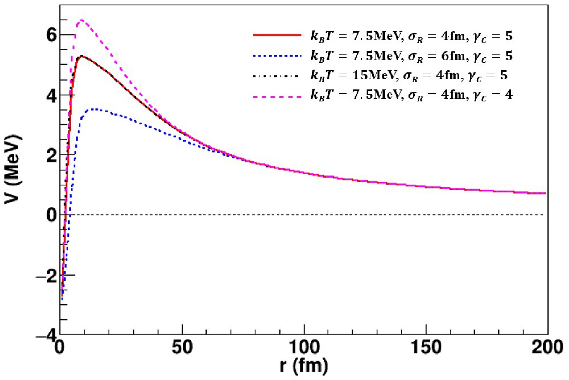
Figure 1. (color online) The mean field experienced by a triton is shown for different values of
$ k_{{\rm{B}}}T $ ,$ \sigma_{{\rm{R}}} $ , and$ \gamma_{{\rm{c}}} $ . Here,$ \gamma_{\rm{d}}=0.3 $ and$ U_0=3 $ MeV are fixed, and the reaction system is 86Kr+208Pb. -
As mentioned above, an initial state of thermal equilibrium is assumed in the calculation. Considering the central-force potential of the residual nucleus, we construct the mean field from a general expression that can be divided into three parts.
(i) Electric term. Since a point charge is unphysical at such small scales, we model the positive charge as having a finite density distribution. To maintain generality, we assume that the positive charge density follows a spherically symmetric Gaussian distribution. That is,
$ \rho_+(\boldsymbol{r})=Z_{{\rm{res}}}\mathfrak{e}(2\pi\sigma_{c}^2)^{-\frac{3}{2}}\exp{\left[-\frac{r^2}{2\sigma_{{\rm{c}}}^2}\right]}, $
(13) where
$ Z_{{\rm{res}}} $ is the residual charge number and$ \mathfrak{e} $ is the unit charge.$ \sigma_{{\rm{c}}} $ characterizes the spatial extent of the charge distribution that generates the Coulomb potential. Solving the Poisson equation and multiplying by the charge of the emitted particle, we obtain$ V_{{\rm{c}}}(r)=\alpha\frac{1}{r}{{\rm{erf}}}(\frac{r}{\sqrt{2}\sigma_{{\rm{c}}}}), $
(14) where
$ \alpha=\dfrac{Z_{{\rm{res}}}Z_{1}\mathfrak{e}^2}{4\pi\epsilon_0} $ and$ {{\rm{erf}}}(x) $ is the Gaussian error function.(ii) Volume term. This contribution originates from the effective nuclear force, and the volume potential is always taken to have the Woods–Saxon form,
$ V_{{\rm{v}}}(r)=\frac{V_0}{1+\exp{\left(\dfrac{r-r_0}{d}\right)}}. $
(15) Let
$ \beta={\mathrm{e}}^{-r_0/d} $ , one obtains$ V_{{\rm{v}}}(r)=\frac{V_0}{1+\beta \exp{(r/d)}}, $
(16) where
$ V_0, r_0 $ , and d are three parameters. Here,$ V_0 $ denotes the depth of the potential well, while$ r_0 $ and d denote the effective radius and surface diffuseness parameter, respectively. Since$ r_0 $ and d are positive, the inequality$ 0<\beta<1 $ is always satisfied.(iii) Surface term. As in the treatment of surface absorption in the optical model, this term is expressed as the derivative of the Woods-Saxon function,
$ V_{{\rm{s}}}(r)=\frac{S_0 \exp{(r/d)}}{\left[1+\beta \exp{(r/d)}\right]^2}. $
(17) The mean field can then be represented as
$ V_{{\rm{MF}}}=V_{{\rm{c}}}+V_{{\rm{v}}}+V_{{\rm{s}}}, $
(18) where r is the distance between the particle and the origin.
Here, the source potential contains six microscopic parameters:
$ \sigma_{{\rm{c}}} $ ,$ V_0 $ ,$ S_0 $ , d, β, and$ U_0 $ . These parameters can be determined as follows.$ (1) $ As$ r\rightarrow \infty $ ,$ V_{{\rm{MF}}} $ must approach a pure Coulomb potential. This condition leads directly to$ \alpha=z_1Z_{{\rm{res}}}\mathfrak{e}^2/4\pi\epsilon_0 $ , where$ z_1 $ is the charge number of the emitted particle.$ (2) $ As$ r\rightarrow 0 $ ,$ V_{{\rm{MF}}} $ must behave as a harmonic-oscillator potential. In this limit, the potential can be constructed by applying Taylor expansions to (14), (16), and (17).$ V_{{\rm{c}}}(r)=\frac{\alpha}{\sigma_{{\rm{c}}}}\sqrt{\frac{2}{\pi}}(1-\frac{1}{6\sigma_{{\rm{c}}}^{2}}r^2)+O(r^{3}), $
(19) $ V_{{\rm{v}}}(r)=\frac{V_0}{1+\beta}(1-\frac{\beta}{(1+\beta)d}r-\frac{\beta(1-\beta)}{2(1+\beta)^2d^2}r^2)+O(r^{3}), $
(20) $ V_{{\rm{s}}}(r)=\frac{S_0}{(1+\beta)^2}(1+\frac{1-\beta}{(1+\beta)d}r+\frac{1-4\beta+\beta^2}{2(1+\beta)^2d^2}r^2)+O(r^{3}). $
(21) To treat the Gaussian source in thermal equilibrium self-consistently, we set the r term to 0 and the coefficient of the
$ r^2 $ term to$ \dfrac{k_{{\rm{B}}}T}{\sigma_{{\rm{R}}}^2} $ . By combining (10), (18), (19), (20), and (21), we derive the following constraint.$ \frac{\alpha}{\sigma_{{\rm{c}}}}\sqrt{\frac{2}{\pi}}+\frac{V_0}{1+\beta}+\frac{s}{(1+\beta)^2}=-U_0, $
(22) $ -\frac{V_0}{1+\beta}\frac{\beta}{(1+\beta)d}+\frac{S_0}{(1+\beta)^2}\frac{1-\beta}{(1+\beta)d}=0, $
(23) $ \begin{aligned}[b]& -\frac{\alpha}{6\sigma_{{\rm{c}}}^{3}}\sqrt{\frac{2}{\pi}}-\frac{V_0}{1+\beta}\frac{\beta(1-\beta)}{2(1+\beta)^2d^2} +\frac{S_0}{(1+\beta)^2}\frac{1-4\beta+\beta^2}{2(1+\beta)^2d^2}=\frac{k_{{\rm{B}}}T}{2\sigma_{{\rm{R}}}^2}. \end{aligned} $
(24) Here we define that
$ \sigma_{{\rm{c}}}=\gamma_{{\rm{c}}}\sigma_{{\rm{R}}}, $
(25) $ d=\gamma_{{\rm{d}}}\sigma_{{\rm{R}}}, $
(26) $ U_{{\rm{c}}}=\frac{\alpha}{\sigma_{{\rm{c}}}}\sqrt{\frac{2}{\pi}}, $
(27) and to solve the constraint equations, one writes
$ V_0=-(U_{{\rm{c}}}+U_0)(1+\beta)(1-\beta), $
(28) $ S_0=-(U_{{\rm{c}}}+U_0)\beta(1+\beta)^2, $
(29) $ \frac{\gamma_{{\rm{d}}}^2 U_{{\rm{c}}}}{U_{{\rm{c}}}+U_0}\left(\frac{k_{{\rm{B}}}T}{2U_{{\rm{c}}}}+\frac{1}{6\gamma_{{\rm{c}}}^2}\right)=\frac{\beta^2}{(1+\beta)^2}. $
(30) If
$ \gamma_{{\rm{c}}} $ and$ \gamma_{{\rm{d}}} $ are chosen as free parameters, the model has only three parameters. However, the constraint$ 0< \beta \lt 1 $ must be satisfied, which leads to the following inequality:$ \frac{\gamma_{{\rm{d}}}^2 U_{{\rm{c}}}}{U_{{\rm{c}}}+U_0}\left(\frac{k_{{\rm{B}}}T}{2U_{{\rm{c}}}}+\frac{1}{6\gamma_{{\rm{c}}}^2}\right)< \frac{1}{4}. $
(31) Given the six initial parameters and the three derived constraints, namely Eq. (28), Eq. (29), and Eq. (30), three free parameters remain. One can choose
$ \gamma_{{\rm{c}}} $ ,$ \gamma_{{\rm{d}}} $ , and$ U_0 $ as the free parameters for the potential, while T and$ \sigma_{{\rm{R}}} $ are taken as input quantities that define the characteristics of the thermal equilibrium emitting source.Up to now, we have defined the emitting source as a thermal equilibrium fireball with temperature
$ k_{\rm{B}}T $ and Gaussian source size$ \sigma_{{\rm{R}}} $ , where the charge distribution follows a Gaussian form with standard deviation$ \sigma_{\rm{c}} $ . The core, which provides the attractive nuclear interaction, is governed by a trapping potential characterized by$ U_0 $ , and surface diffusion is described by the coefficient d.Figure 1 presents a set of potentials with different parameter values. The temperature
$ k_{{\rm{B}}}T $ produces almost no difference, which is consistent with the expectation that the temperature should not affect the potential. The Gaussian source size$ \sigma_{{\rm{R}}} $ affects both the position and the height of the peak, whereas$ \gamma_{{\rm{c}}} $ influences only the height.
Figure 1. (color online) The mean field experienced by a triton is shown for different values of
$ k_{{\rm{B}}}T $ ,$ \sigma_{{\rm{R}}} $ , and$ \gamma_{{\rm{c}}} $ . Here,$ \gamma_{\rm{d}}=0.3 $ and$ U_0=3 $ MeV are fixed, and the reaction system is 86Kr+208Pb. -
As mentioned above, an initial state of thermal equilibrium is assumed in the calculation. Considering the central-force potential of the residual nucleus, we construct the mean field from a general expression that can be divided into three parts.
(i) Electric term. Since a point charge is unphysical at such small scales, we model the positive charge as having a finite density distribution. To maintain generality, we assume that the positive charge density follows a spherically symmetric Gaussian distribution. That is,
$ \rho_+(\boldsymbol{r})=Z_{{\rm{res}}}\mathfrak{e}(2\pi\sigma_{c}^2)^{-\frac{3}{2}}\exp{\left[-\frac{r^2}{2\sigma_{{\rm{c}}}^2}\right]}, $
(13) where
$ Z_{{\rm{res}}} $ is the residual charge number and$ \mathfrak{e} $ is the unit charge.$ \sigma_{{\rm{c}}} $ characterizes the spatial extent of the charge distribution that generates the Coulomb potential. Solving the Poisson equation and multiplying by the charge of the emitted particle, we obtain$ V_{{\rm{c}}}(r)=\alpha\frac{1}{r}{{\rm{erf}}}(\frac{r}{\sqrt{2}\sigma_{{\rm{c}}}}), $
(14) where
$ \alpha=\dfrac{Z_{{\rm{res}}}Z_{1}\mathfrak{e}^2}{4\pi\epsilon_0} $ and$ {{\rm{erf}}}(x) $ is the Gaussian error function.(ii) Volume term. This contribution originates from the effective nuclear force, and the volume potential is always taken to have the Woods–Saxon form,
$ V_{{\rm{v}}}(r)=\frac{V_0}{1+\exp{\left(\dfrac{r-r_0}{d}\right)}}. $
(15) Let
$ \beta={\mathrm{e}}^{-r_0/d} $ , one obtains$ V_{{\rm{v}}}(r)=\frac{V_0}{1+\beta \exp{(r/d)}}, $
(16) where
$ V_0, r_0 $ , and d are three parameters. Here,$ V_0 $ denotes the depth of the potential well, while$ r_0 $ and d denote the effective radius and surface diffuseness parameter, respectively. Since$ r_0 $ and d are positive, the inequality$ 0<\beta<1 $ is always satisfied.(iii) Surface term. As in the treatment of surface absorption in the optical model, this term is expressed as the derivative of the Woods-Saxon function,
$ V_{{\rm{s}}}(r)=\frac{S_0 \exp{(r/d)}}{\left[1+\beta \exp{(r/d)}\right]^2}. $
(17) The mean field can then be represented as
$ V_{{\rm{MF}}}=V_{{\rm{c}}}+V_{{\rm{v}}}+V_{{\rm{s}}}, $
(18) where r is the distance between the particle and the origin.
Here, the source potential contains six microscopic parameters:
$ \sigma_{{\rm{c}}} $ ,$ V_0 $ ,$ S_0 $ , d, β, and$ U_0 $ . These parameters can be determined as follows.$ (1) $ As$ r\rightarrow \infty $ ,$ V_{{\rm{MF}}} $ must approach a pure Coulomb potential. This condition leads directly to$ \alpha=z_1Z_{{\rm{res}}}\mathfrak{e}^2/4\pi\epsilon_0 $ , where$ z_1 $ is the charge number of the emitted particle.$ (2) $ As$ r\rightarrow 0 $ ,$ V_{{\rm{MF}}} $ must behave as a harmonic-oscillator potential. In this limit, the potential can be constructed by applying Taylor expansions to (14), (16), and (17).$ V_{{\rm{c}}}(r)=\frac{\alpha}{\sigma_{{\rm{c}}}}\sqrt{\frac{2}{\pi}}(1-\frac{1}{6\sigma_{{\rm{c}}}^{2}}r^2)+O(r^{3}), $
(19) $ V_{{\rm{v}}}(r)=\frac{V_0}{1+\beta}(1-\frac{\beta}{(1+\beta)d}r-\frac{\beta(1-\beta)}{2(1+\beta)^2d^2}r^2)+O(r^{3}), $
(20) $ V_{{\rm{s}}}(r)=\frac{S_0}{(1+\beta)^2}(1+\frac{1-\beta}{(1+\beta)d}r+\frac{1-4\beta+\beta^2}{2(1+\beta)^2d^2}r^2)+O(r^{3}). $
(21) To treat the Gaussian source in thermal equilibrium self-consistently, we set the r term to 0 and the coefficient of the
$ r^2 $ term to$ \dfrac{k_{{\rm{B}}}T}{\sigma_{{\rm{R}}}^2} $ . By combining (10), (18), (19), (20), and (21), we derive the following constraint.$ \frac{\alpha}{\sigma_{{\rm{c}}}}\sqrt{\frac{2}{\pi}}+\frac{V_0}{1+\beta}+\frac{s}{(1+\beta)^2}=-U_0, $
(22) $ -\frac{V_0}{1+\beta}\frac{\beta}{(1+\beta)d}+\frac{S_0}{(1+\beta)^2}\frac{1-\beta}{(1+\beta)d}=0, $
(23) $ \begin{aligned}[b]& -\frac{\alpha}{6\sigma_{{\rm{c}}}^{3}}\sqrt{\frac{2}{\pi}}-\frac{V_0}{1+\beta}\frac{\beta(1-\beta)}{2(1+\beta)^2d^2} +\frac{S_0}{(1+\beta)^2}\frac{1-4\beta+\beta^2}{2(1+\beta)^2d^2}=\frac{k_{{\rm{B}}}T}{2\sigma_{{\rm{R}}}^2}. \end{aligned} $
(24) Here we define that
$ \sigma_{{\rm{c}}}=\gamma_{{\rm{c}}}\sigma_{{\rm{R}}}, $
(25) $ d=\gamma_{{\rm{d}}}\sigma_{{\rm{R}}}, $
(26) $ U_{{\rm{c}}}=\frac{\alpha}{\sigma_{{\rm{c}}}}\sqrt{\frac{2}{\pi}}, $
(27) and to solve the constraint equations, one writes
$ V_0=-(U_{{\rm{c}}}+U_0)(1+\beta)(1-\beta), $
(28) $ S_0=-(U_{{\rm{c}}}+U_0)\beta(1+\beta)^2, $
(29) $ \frac{\gamma_{{\rm{d}}}^2 U_{{\rm{c}}}}{U_{{\rm{c}}}+U_0}\left(\frac{k_{{\rm{B}}}T}{2U_{{\rm{c}}}}+\frac{1}{6\gamma_{{\rm{c}}}^2}\right)=\frac{\beta^2}{(1+\beta)^2}. $
(30) If
$ \gamma_{{\rm{c}}} $ and$ \gamma_{{\rm{d}}} $ are chosen as free parameters, the model has only three parameters. However, the constraint$ 0< \beta \lt 1 $ must be satisfied, which leads to the following inequality:$ \frac{\gamma_{{\rm{d}}}^2 U_{{\rm{c}}}}{U_{{\rm{c}}}+U_0}\left(\frac{k_{{\rm{B}}}T}{2U_{{\rm{c}}}}+\frac{1}{6\gamma_{{\rm{c}}}^2}\right)< \frac{1}{4}. $
(31) Given the six initial parameters and the three derived constraints, namely Eq. (28), Eq. (29), and Eq. (30), three free parameters remain. One can choose
$ \gamma_{{\rm{c}}} $ ,$ \gamma_{{\rm{d}}} $ , and$ U_0 $ as the free parameters for the potential, while T and$ \sigma_{{\rm{R}}} $ are taken as input quantities that define the characteristics of the thermal equilibrium emitting source.Up to now, we have defined the emitting source as a thermal equilibrium fireball with temperature
$ k_{\rm{B}}T $ and Gaussian source size$ \sigma_{{\rm{R}}} $ , where the charge distribution follows a Gaussian form with standard deviation$ \sigma_{\rm{c}} $ . The core, which provides the attractive nuclear interaction, is governed by a trapping potential characterized by$ U_0 $ , and surface diffusion is described by the coefficient d.Figure 1 presents a set of potentials with different parameter values. The temperature
$ k_{{\rm{B}}}T $ produces almost no difference, which is consistent with the expectation that the temperature should not affect the potential. The Gaussian source size$ \sigma_{{\rm{R}}} $ affects both the position and the height of the peak, whereas$ \gamma_{{\rm{c}}} $ influences only the height.
Figure 1. (color online) The mean field experienced by a triton is shown for different values of
$ k_{{\rm{B}}}T $ ,$ \sigma_{{\rm{R}}} $ , and$ \gamma_{{\rm{c}}} $ . Here,$ \gamma_{\rm{d}}=0.3 $ and$ U_0=3 $ MeV are fixed, and the reaction system is 86Kr+208Pb. -
As mentioned above, an initial state of thermal equilibrium is assumed in the calculation. Considering the central-force potential of the residual nucleus, we construct the mean field from a general expression that can be divided into three parts.
(i) Electric term. Since a point charge is unphysical at such small scales, we model the positive charge as having a finite density distribution. To maintain generality, we assume that the positive charge density follows a spherically symmetric Gaussian distribution. That is,
$ \rho_+(\boldsymbol{r})=Z_{{\rm{res}}}\mathfrak{e}(2\pi\sigma_{c}^2)^{-\frac{3}{2}}\exp{\left[-\frac{r^2}{2\sigma_{{\rm{c}}}^2}\right]}, $
(13) where
$ Z_{{\rm{res}}} $ is the residual charge number and$ \mathfrak{e} $ is the unit charge.$ \sigma_{{\rm{c}}} $ characterizes the spatial extent of the charge distribution that generates the Coulomb potential. Solving the Poisson equation and multiplying by the charge of the emitted particle, we obtain$ V_{{\rm{c}}}(r)=\alpha\frac{1}{r}{{\rm{erf}}}(\frac{r}{\sqrt{2}\sigma_{{\rm{c}}}}), $
(14) where
$ \alpha=\dfrac{Z_{{\rm{res}}}Z_{1}\mathfrak{e}^2}{4\pi\epsilon_0} $ and$ {{\rm{erf}}}(x) $ is the Gaussian error function.(ii) Volume term. This contribution originates from the effective nuclear force, and the volume potential is always taken to have the Woods–Saxon form,
$ V_{{\rm{v}}}(r)=\frac{V_0}{1+\exp{\left(\dfrac{r-r_0}{d}\right)}}. $
(15) Let
$ \beta={\mathrm{e}}^{-r_0/d} $ , one obtains$ V_{{\rm{v}}}(r)=\frac{V_0}{1+\beta \exp{(r/d)}}, $
(16) where
$ V_0, r_0 $ , and d are three parameters. Here,$ V_0 $ denotes the depth of the potential well, while$ r_0 $ and d denote the effective radius and surface diffuseness parameter, respectively. Since$ r_0 $ and d are positive, the inequality$ 0<\beta<1 $ is always satisfied.(iii) Surface term. As in the treatment of surface absorption in the optical model, this term is expressed as the derivative of the Woods-Saxon function,
$ V_{{\rm{s}}}(r)=\frac{S_0 \exp{(r/d)}}{\left[1+\beta \exp{(r/d)}\right]^2}. $
(17) The mean field can then be represented as
$ V_{{\rm{MF}}}=V_{{\rm{c}}}+V_{{\rm{v}}}+V_{{\rm{s}}}, $
(18) where r is the distance between the particle and the origin.
Here, the source potential contains six microscopic parameters:
$ \sigma_{{\rm{c}}} $ ,$ V_0 $ ,$ S_0 $ , d, β, and$ U_0 $ . These parameters can be determined as follows.$ (1) $ As$ r\rightarrow \infty $ ,$ V_{{\rm{MF}}} $ must approach a pure Coulomb potential. This condition leads directly to$ \alpha=z_1Z_{{\rm{res}}}\mathfrak{e}^2/4\pi\epsilon_0 $ , where$ z_1 $ is the charge number of the emitted particle.$ (2) $ As$ r\rightarrow 0 $ ,$ V_{{\rm{MF}}} $ must behave as a harmonic-oscillator potential. In this limit, the potential can be constructed by applying Taylor expansions to (14), (16), and (17).$ V_{{\rm{c}}}(r)=\frac{\alpha}{\sigma_{{\rm{c}}}}\sqrt{\frac{2}{\pi}}(1-\frac{1}{6\sigma_{{\rm{c}}}^{2}}r^2)+O(r^{3}), $
(19) $ V_{{\rm{v}}}(r)=\frac{V_0}{1+\beta}(1-\frac{\beta}{(1+\beta)d}r-\frac{\beta(1-\beta)}{2(1+\beta)^2d^2}r^2)+O(r^{3}), $
(20) $ V_{{\rm{s}}}(r)=\frac{S_0}{(1+\beta)^2}(1+\frac{1-\beta}{(1+\beta)d}r+\frac{1-4\beta+\beta^2}{2(1+\beta)^2d^2}r^2)+O(r^{3}). $
(21) To treat the Gaussian source in thermal equilibrium self-consistently, we set the r term to 0 and the coefficient of the
$ r^2 $ term to$ \dfrac{k_{{\rm{B}}}T}{\sigma_{{\rm{R}}}^2} $ . By combining (10), (18), (19), (20), and (21), we derive the following constraint.$ \frac{\alpha}{\sigma_{{\rm{c}}}}\sqrt{\frac{2}{\pi}}+\frac{V_0}{1+\beta}+\frac{s}{(1+\beta)^2}=-U_0, $
(22) $ -\frac{V_0}{1+\beta}\frac{\beta}{(1+\beta)d}+\frac{S_0}{(1+\beta)^2}\frac{1-\beta}{(1+\beta)d}=0, $
(23) $ \begin{aligned}[b]& -\frac{\alpha}{6\sigma_{{\rm{c}}}^{3}}\sqrt{\frac{2}{\pi}}-\frac{V_0}{1+\beta}\frac{\beta(1-\beta)}{2(1+\beta)^2d^2} +\frac{S_0}{(1+\beta)^2}\frac{1-4\beta+\beta^2}{2(1+\beta)^2d^2}=\frac{k_{{\rm{B}}}T}{2\sigma_{{\rm{R}}}^2}. \end{aligned} $
(24) Here we define that
$ \sigma_{{\rm{c}}}=\gamma_{{\rm{c}}}\sigma_{{\rm{R}}}, $
(25) $ d=\gamma_{{\rm{d}}}\sigma_{{\rm{R}}}, $
(26) $ U_{{\rm{c}}}=\frac{\alpha}{\sigma_{{\rm{c}}}}\sqrt{\frac{2}{\pi}}, $
(27) and to solve the constraint equations, one writes
$ V_0=-(U_{{\rm{c}}}+U_0)(1+\beta)(1-\beta), $
(28) $ S_0=-(U_{{\rm{c}}}+U_0)\beta(1+\beta)^2, $
(29) $ \frac{\gamma_{{\rm{d}}}^2 U_{{\rm{c}}}}{U_{{\rm{c}}}+U_0}\left(\frac{k_{{\rm{B}}}T}{2U_{{\rm{c}}}}+\frac{1}{6\gamma_{{\rm{c}}}^2}\right)=\frac{\beta^2}{(1+\beta)^2}. $
(30) If
$ \gamma_{{\rm{c}}} $ and$ \gamma_{{\rm{d}}} $ are chosen as free parameters, the model has only three parameters. However, the constraint$ 0< \beta \lt 1 $ must be satisfied, which leads to the following inequality:$ \frac{\gamma_{{\rm{d}}}^2 U_{{\rm{c}}}}{U_{{\rm{c}}}+U_0}\left(\frac{k_{{\rm{B}}}T}{2U_{{\rm{c}}}}+\frac{1}{6\gamma_{{\rm{c}}}^2}\right)< \frac{1}{4}. $
(31) Given the six initial parameters and the three derived constraints, namely Eq. (28), Eq. (29), and Eq. (30), three free parameters remain. One can choose
$ \gamma_{{\rm{c}}} $ ,$ \gamma_{{\rm{d}}} $ , and$ U_0 $ as the free parameters for the potential, while T and$ \sigma_{{\rm{R}}} $ are taken as input quantities that define the characteristics of the thermal equilibrium emitting source.Up to now, we have defined the emitting source as a thermal equilibrium fireball with temperature
$ k_{\rm{B}}T $ and Gaussian source size$ \sigma_{{\rm{R}}} $ , where the charge distribution follows a Gaussian form with standard deviation$ \sigma_{\rm{c}} $ . The core, which provides the attractive nuclear interaction, is governed by a trapping potential characterized by$ U_0 $ , and surface diffusion is described by the coefficient d.Figure 1 presents a set of potentials with different parameter values. The temperature
$ k_{{\rm{B}}}T $ produces almost no difference, which is consistent with the expectation that the temperature should not affect the potential. The Gaussian source size$ \sigma_{{\rm{R}}} $ affects both the position and the height of the peak, whereas$ \gamma_{{\rm{c}}} $ influences only the height.
Figure 1. (color online) The mean field experienced by a triton is shown for different values of
$ k_{{\rm{B}}}T $ ,$ \sigma_{{\rm{R}}} $ , and$ \gamma_{{\rm{c}}} $ . Here,$ \gamma_{\rm{d}}=0.3 $ and$ U_0=3 $ MeV are fixed, and the reaction system is 86Kr+208Pb. -
As mentioned above, an initial state of thermal equilibrium is assumed in the calculation. Considering the central-force potential of the residual nucleus, we construct the mean field from a general expression that can be divided into three parts.
(i) Electric term. Since a point charge is unphysical at such small scales, we model the positive charge as having a finite density distribution. To maintain generality, we assume that the positive charge density follows a spherically symmetric Gaussian distribution. That is,
$ \rho_+(\boldsymbol{r})=Z_{{\rm{res}}}\mathfrak{e}(2\pi\sigma_{c}^2)^{-\frac{3}{2}}\exp{\left[-\frac{r^2}{2\sigma_{{\rm{c}}}^2}\right]}, $
(13) where
$ Z_{{\rm{res}}} $ is the residual charge number and$ \mathfrak{e} $ is the unit charge.$ \sigma_{{\rm{c}}} $ characterizes the spatial extent of the charge distribution that generates the Coulomb potential. Solving the Poisson equation and multiplying by the charge of the emitted particle, we obtain$ V_{{\rm{c}}}(r)=\alpha\frac{1}{r}{{\rm{erf}}}(\frac{r}{\sqrt{2}\sigma_{{\rm{c}}}}), $
(14) where
$ \alpha=\dfrac{Z_{{\rm{res}}}Z_{1}\mathfrak{e}^2}{4\pi\epsilon_0} $ and$ {{\rm{erf}}}(x) $ is the Gaussian error function.(ii) Volume term. This contribution originates from the effective nuclear force, and the volume potential is always taken to have the Woods–Saxon form,
$ V_{{\rm{v}}}(r)=\frac{V_0}{1+\exp{\left(\dfrac{r-r_0}{d}\right)}}. $
(15) Let
$ \beta={\mathrm{e}}^{-r_0/d} $ , one obtains$ V_{{\rm{v}}}(r)=\frac{V_0}{1+\beta \exp{(r/d)}}, $
(16) where
$ V_0, r_0 $ , and d are three parameters. Here,$ V_0 $ denotes the depth of the potential well, while$ r_0 $ and d denote the effective radius and surface diffuseness parameter, respectively. Since$ r_0 $ and d are positive, the inequality$ 0<\beta<1 $ is always satisfied.(iii) Surface term. As in the treatment of surface absorption in the optical model, this term is expressed as the derivative of the Woods-Saxon function,
$ V_{{\rm{s}}}(r)=\frac{S_0 \exp{(r/d)}}{\left[1+\beta \exp{(r/d)}\right]^2}. $
(17) The mean field can then be represented as
$ V_{{\rm{MF}}}=V_{{\rm{c}}}+V_{{\rm{v}}}+V_{{\rm{s}}}, $
(18) where r is the distance between the particle and the origin.
Here, the source potential contains six microscopic parameters:
$ \sigma_{{\rm{c}}} $ ,$ V_0 $ ,$ S_0 $ , d, β, and$ U_0 $ . These parameters can be determined as follows.$ (1) $ As$ r\rightarrow \infty $ ,$ V_{{\rm{MF}}} $ must approach a pure Coulomb potential. This condition leads directly to$ \alpha=z_1Z_{{\rm{res}}}\mathfrak{e}^2/4\pi\epsilon_0 $ , where$ z_1 $ is the charge number of the emitted particle.$ (2) $ As$ r\rightarrow 0 $ ,$ V_{{\rm{MF}}} $ must behave as a harmonic-oscillator potential. In this limit, the potential can be constructed by applying Taylor expansions to (14), (16), and (17).$ V_{{\rm{c}}}(r)=\frac{\alpha}{\sigma_{{\rm{c}}}}\sqrt{\frac{2}{\pi}}(1-\frac{1}{6\sigma_{{\rm{c}}}^{2}}r^2)+O(r^{3}), $
(19) $ V_{{\rm{v}}}(r)=\frac{V_0}{1+\beta}(1-\frac{\beta}{(1+\beta)d}r-\frac{\beta(1-\beta)}{2(1+\beta)^2d^2}r^2)+O(r^{3}), $
(20) $ V_{{\rm{s}}}(r)=\frac{S_0}{(1+\beta)^2}(1+\frac{1-\beta}{(1+\beta)d}r+\frac{1-4\beta+\beta^2}{2(1+\beta)^2d^2}r^2)+O(r^{3}). $
(21) To treat the Gaussian source in thermal equilibrium self-consistently, we set the r term to 0 and the coefficient of the
$ r^2 $ term to$ \dfrac{k_{{\rm{B}}}T}{\sigma_{{\rm{R}}}^2} $ . By combining (10), (18), (19), (20), and (21), we derive the following constraint.$ \frac{\alpha}{\sigma_{{\rm{c}}}}\sqrt{\frac{2}{\pi}}+\frac{V_0}{1+\beta}+\frac{s}{(1+\beta)^2}=-U_0, $
(22) $ -\frac{V_0}{1+\beta}\frac{\beta}{(1+\beta)d}+\frac{S_0}{(1+\beta)^2}\frac{1-\beta}{(1+\beta)d}=0, $
(23) $ \begin{aligned}[b]& -\frac{\alpha}{6\sigma_{{\rm{c}}}^{3}}\sqrt{\frac{2}{\pi}}-\frac{V_0}{1+\beta}\frac{\beta(1-\beta)}{2(1+\beta)^2d^2} +\frac{S_0}{(1+\beta)^2}\frac{1-4\beta+\beta^2}{2(1+\beta)^2d^2}=\frac{k_{{\rm{B}}}T}{2\sigma_{{\rm{R}}}^2}. \end{aligned} $
(24) Here we define that
$ \sigma_{{\rm{c}}}=\gamma_{{\rm{c}}}\sigma_{{\rm{R}}}, $
(25) $ d=\gamma_{{\rm{d}}}\sigma_{{\rm{R}}}, $
(26) $ U_{{\rm{c}}}=\frac{\alpha}{\sigma_{{\rm{c}}}}\sqrt{\frac{2}{\pi}}, $
(27) and to solve the constraint equations, one writes
$ V_0=-(U_{{\rm{c}}}+U_0)(1+\beta)(1-\beta), $
(28) $ S_0=-(U_{{\rm{c}}}+U_0)\beta(1+\beta)^2, $
(29) $ \frac{\gamma_{{\rm{d}}}^2 U_{{\rm{c}}}}{U_{{\rm{c}}}+U_0}\left(\frac{k_{{\rm{B}}}T}{2U_{{\rm{c}}}}+\frac{1}{6\gamma_{{\rm{c}}}^2}\right)=\frac{\beta^2}{(1+\beta)^2}. $
(30) If
$ \gamma_{{\rm{c}}} $ and$ \gamma_{{\rm{d}}} $ are chosen as free parameters, the model has only three parameters. However, the constraint$ 0< \beta \lt 1 $ must be satisfied, which leads to the following inequality:$ \frac{\gamma_{{\rm{d}}}^2 U_{{\rm{c}}}}{U_{{\rm{c}}}+U_0}\left(\frac{k_{{\rm{B}}}T}{2U_{{\rm{c}}}}+\frac{1}{6\gamma_{{\rm{c}}}^2}\right)< \frac{1}{4}. $
(31) Given the six initial parameters and the three derived constraints, namely Eq. (28), Eq. (29), and Eq. (30), three free parameters remain. One can choose
$ \gamma_{{\rm{c}}} $ ,$ \gamma_{{\rm{d}}} $ , and$ U_0 $ as the free parameters for the potential, while T and$ \sigma_{{\rm{R}}} $ are taken as input quantities that define the characteristics of the thermal equilibrium emitting source.Up to now, we have defined the emitting source as a thermal equilibrium fireball with temperature
$ k_{\rm{B}}T $ and Gaussian source size$ \sigma_{{\rm{R}}} $ , where the charge distribution follows a Gaussian form with standard deviation$ \sigma_{\rm{c}} $ . The core, which provides the attractive nuclear interaction, is governed by a trapping potential characterized by$ U_0 $ , and surface diffusion is described by the coefficient d.Figure 1 presents a set of potentials with different parameter values. The temperature
$ k_{{\rm{B}}}T $ produces almost no difference, which is consistent with the expectation that the temperature should not affect the potential. The Gaussian source size$ \sigma_{{\rm{R}}} $ affects both the position and the height of the peak, whereas$ \gamma_{{\rm{c}}} $ influences only the height.
Figure 1. (color online) The mean field experienced by a triton is shown for different values of
$ k_{{\rm{B}}}T $ ,$ \sigma_{{\rm{R}}} $ , and$ \gamma_{{\rm{c}}} $ . Here,$ \gamma_{\rm{d}}=0.3 $ and$ U_0=3 $ MeV are fixed, and the reaction system is 86Kr+208Pb. -
In this subsection, we solve the dynamical evolution and derive the observable, namely the correlation function.
The initial state of the motion can be constructed by random sampling based on the characteristics of the emitting source. The subsequent procedure simulates the dynamics of the correlated particle pair, as described by classical mechanics. Specifically, the trajectories of the emitted particles are evolved over time as a time series, with each time step defined by the interval
$ \Delta t $ . The interactions between the emitted particles and the source are taken into account. For a pair of particles with masses$ (m_1,m_2) $ , their trajectories are described by the time-dependent positions and momenta, denoted by$ {(\boldsymbol{x}_1(t),\boldsymbol{p}_1(t))} $ and$ {(\boldsymbol{x}_2(t),\boldsymbol{p}_2(t))} $ , respectively. The state of the system after one time step is calculated as follows.First, the test movement is calculated as follows.
$ \boldsymbol{x}'_i(t+\Delta t)=\boldsymbol{x}_i(t)+\frac{1}{m_i}\boldsymbol{p}_i(t)\Delta t-\frac{1}{2}\frac{\nabla_i V(\boldsymbol{x}_i;\boldsymbol{x}_j)}{m_i}\Delta t^2 , $
(32) $ \boldsymbol{p}'_i(t+\Delta t)=\boldsymbol{p}_i(t)-\nabla_i V(\boldsymbol{x}_i;\boldsymbol{x}_j))\Delta t , $
(33) where
$ (i,j)\in \{(1,2),(2,1)\} $ .Next, we assume that the average force over a time interval can be constructed by combining the force in the current state with that in the test state. This procedure yields an acceptable displacement of the particle pair for the given time step.
$ \begin{aligned}[b] \boldsymbol{x}_i(t+\Delta t)=&\boldsymbol{x}_i(t)+\frac{1}{m_i}\boldsymbol{p}_i(t)\Delta t\\& -\frac{1}{2}\frac{(\gamma \nabla_i V(\boldsymbol{x}_i;\boldsymbol{x}_j)+(1-\gamma)\nabla_i' V(\boldsymbol{x}_i';\boldsymbol{x}_j'))}{m_i}\Delta t^2 ,\end{aligned} $
(34) $ \boldsymbol{p}_i(t+\Delta t)=\boldsymbol{p}_i(t)-(\gamma \nabla_i V(\boldsymbol{x}_i;\boldsymbol{x}_j)+(1-\gamma)\nabla_i' V(\boldsymbol{x}_i';\boldsymbol{x}_j'))\Delta t , $
(35) where
$ (i,j)\in \{(1,2),(2,1)\} $ , and γ is a numerical parameter that balances the force before (subscript 'pre') and after (subscript 'pos') a motion step, satisfying$ F_{{\rm{cal}}}= \gamma F_{{\rm{pre}}}+ (1-\gamma)F_{{\rm{pos}}} $ . We choose$ \gamma=0.5 $ in the calculations.At this stage, the basic framework of the simulation model has been constructed. The final step is to incorporate correlations between the particles. Because we neglect the effects of Bose-Einstein or Fermi-Dirac statistics, the correlations arise solely from dynamical interactions between the particles. The interaction between a pair of particles can be described by their position vectors
$ \boldsymbol{r}_1 $ and$ \boldsymbol{r}_2 $ , which represent the particle positions at a given time. The correlation between the particles is governed by the forces resulting from their relative positions and the dynamics of their interaction.$ V_1(\boldsymbol{r}_1;\boldsymbol{r}_2)=V_{{\rm{MF}}}(r_1)+V_{12}(\boldsymbol{r}_1-\boldsymbol{r}_2) , $
(36) $ V_2(\boldsymbol{r}_2;\boldsymbol{r}_1)=V_{{\rm{MF}}}(r_2)+V_{12}(\boldsymbol{r}_2-\boldsymbol{r}_1) .$
(37) If the interaction between the emitted particle pair contains only the Coulomb interaction, one writes
$ V_{12}(\boldsymbol{r}_{12})=\frac{Z_1 Z_2 \mathfrak{e}^2}{4\pi\epsilon_0}\frac{1}{\boldsymbol{r}_{12}} ,$
(38) where
$ Z_1 $ and$ Z_2 $ are the charge numbers of the particle pair.During a series of runs, a set of final events can be accumulated. The correlation function is then defined as
$ C(q)=1+R(q)=C_{12}\frac{\Sigma Y_{12}(\boldsymbol{p}_1,\boldsymbol{p}_2)}{\Sigma Y_1(\boldsymbol{p}_1)Y_2(\boldsymbol{p}_2)}, $
(39) where
$ \boldsymbol{p}_1,\boldsymbol{p}_2 $ are the laboratory momenta,$ Y_{12} $ is the coincidence yield, and$ Y_1,Y_2 $ are the inclusive single-particle yields. Here,$ q=\mu |\boldsymbol{p}_1/m_1-\boldsymbol{p}_2/m_2| $ is the relative momentum of the correlated pair, where$ \mu=m_1m_2/(m_1+m_2) $ is the reduced mass. The normalization constant$ C_{12} $ is determined by imposing the condition$ C(q)=1 $ at large relative momentum. Experimentally, the correlation function is obtained as the normalized ratio of the relative momentum distribution from the same event to that from mixed events as$ C(q)=C_{12}\frac{Y_{{\rm{same}}}(q)}{Y_{{\rm{mix}}}(q)} , $
(40) where the subscripts 'same' and 'mix' denote same-event and mixed-event quantities, respectively.
-
In this subsection, we solve the dynamical evolution and derive the observable, namely the correlation function.
The initial state of the motion can be constructed by random sampling based on the characteristics of the emitting source. The subsequent procedure simulates the dynamics of the correlated particle pair, as described by classical mechanics. Specifically, the trajectories of the emitted particles are evolved over time as a time series, with each time step defined by the interval
$ \Delta t $ . The interactions between the emitted particles and the source are taken into account. For a pair of particles with masses$ (m_1,m_2) $ , their trajectories are described by the time-dependent positions and momenta, denoted by$ {(\boldsymbol{x}_1(t),\boldsymbol{p}_1(t))} $ and$ {(\boldsymbol{x}_2(t),\boldsymbol{p}_2(t))} $ , respectively. The state of the system after one time step is calculated as follows.First, the test movement is calculated as follows.
$ \boldsymbol{x}'_i(t+\Delta t)=\boldsymbol{x}_i(t)+\frac{1}{m_i}\boldsymbol{p}_i(t)\Delta t-\frac{1}{2}\frac{\nabla_i V(\boldsymbol{x}_i;\boldsymbol{x}_j)}{m_i}\Delta t^2 , $
(32) $ \boldsymbol{p}'_i(t+\Delta t)=\boldsymbol{p}_i(t)-\nabla_i V(\boldsymbol{x}_i;\boldsymbol{x}_j))\Delta t , $
(33) where
$ (i,j)\in \{(1,2),(2,1)\} $ .Next, we assume that the average force over a time interval can be constructed by combining the force in the current state with that in the test state. This procedure yields an acceptable displacement of the particle pair for the given time step.
$ \begin{aligned}[b] \boldsymbol{x}_i(t+\Delta t)=&\boldsymbol{x}_i(t)+\frac{1}{m_i}\boldsymbol{p}_i(t)\Delta t\\& -\frac{1}{2}\frac{(\gamma \nabla_i V(\boldsymbol{x}_i;\boldsymbol{x}_j)+(1-\gamma)\nabla_i' V(\boldsymbol{x}_i';\boldsymbol{x}_j'))}{m_i}\Delta t^2 ,\end{aligned} $
(34) $ \boldsymbol{p}_i(t+\Delta t)=\boldsymbol{p}_i(t)-(\gamma \nabla_i V(\boldsymbol{x}_i;\boldsymbol{x}_j)+(1-\gamma)\nabla_i' V(\boldsymbol{x}_i';\boldsymbol{x}_j'))\Delta t , $
(35) where
$ (i,j)\in \{(1,2),(2,1)\} $ , and γ is a numerical parameter that balances the force before (subscript 'pre') and after (subscript 'pos') a motion step, satisfying$ F_{{\rm{cal}}}= \gamma F_{{\rm{pre}}}+ (1-\gamma)F_{{\rm{pos}}} $ . We choose$ \gamma=0.5 $ in the calculations.At this stage, the basic framework of the simulation model has been constructed. The final step is to incorporate correlations between the particles. Because we neglect the effects of Bose-Einstein or Fermi-Dirac statistics, the correlations arise solely from dynamical interactions between the particles. The interaction between a pair of particles can be described by their position vectors
$ \boldsymbol{r}_1 $ and$ \boldsymbol{r}_2 $ , which represent the particle positions at a given time. The correlation between the particles is governed by the forces resulting from their relative positions and the dynamics of their interaction.$ V_1(\boldsymbol{r}_1;\boldsymbol{r}_2)=V_{{\rm{MF}}}(r_1)+V_{12}(\boldsymbol{r}_1-\boldsymbol{r}_2) , $
(36) $ V_2(\boldsymbol{r}_2;\boldsymbol{r}_1)=V_{{\rm{MF}}}(r_2)+V_{12}(\boldsymbol{r}_2-\boldsymbol{r}_1) .$
(37) If the interaction between the emitted particle pair contains only the Coulomb interaction, one writes
$ V_{12}(\boldsymbol{r}_{12})=\frac{Z_1 Z_2 \mathfrak{e}^2}{4\pi\epsilon_0}\frac{1}{\boldsymbol{r}_{12}} ,$
(38) where
$ Z_1 $ and$ Z_2 $ are the charge numbers of the particle pair.During a series of runs, a set of final events can be accumulated. The correlation function is then defined as
$ C(q)=1+R(q)=C_{12}\frac{\Sigma Y_{12}(\boldsymbol{p}_1,\boldsymbol{p}_2)}{\Sigma Y_1(\boldsymbol{p}_1)Y_2(\boldsymbol{p}_2)}, $
(39) where
$ \boldsymbol{p}_1,\boldsymbol{p}_2 $ are the laboratory momenta,$ Y_{12} $ is the coincidence yield, and$ Y_1,Y_2 $ are the inclusive single-particle yields. Here,$ q=\mu |\boldsymbol{p}_1/m_1-\boldsymbol{p}_2/m_2| $ is the relative momentum of the correlated pair, where$ \mu=m_1m_2/(m_1+m_2) $ is the reduced mass. The normalization constant$ C_{12} $ is determined by imposing the condition$ C(q)=1 $ at large relative momentum. Experimentally, the correlation function is obtained as the normalized ratio of the relative momentum distribution from the same event to that from mixed events as$ C(q)=C_{12}\frac{Y_{{\rm{same}}}(q)}{Y_{{\rm{mix}}}(q)} , $
(40) where the subscripts 'same' and 'mix' denote same-event and mixed-event quantities, respectively.
-
In this subsection, we solve the dynamical evolution and derive the observable, namely the correlation function.
The initial state of the motion can be constructed by random sampling based on the characteristics of the emitting source. The subsequent procedure simulates the dynamics of the correlated particle pair, as described by classical mechanics. Specifically, the trajectories of the emitted particles are evolved over time as a time series, with each time step defined by the interval
$ \Delta t $ . The interactions between the emitted particles and the source are taken into account. For a pair of particles with masses$ (m_1,m_2) $ , their trajectories are described by the time-dependent positions and momenta, denoted by$ {(\boldsymbol{x}_1(t),\boldsymbol{p}_1(t))} $ and$ {(\boldsymbol{x}_2(t),\boldsymbol{p}_2(t))} $ , respectively. The state of the system after one time step is calculated as follows.First, the test movement is calculated as follows.
$ \boldsymbol{x}'_i(t+\Delta t)=\boldsymbol{x}_i(t)+\frac{1}{m_i}\boldsymbol{p}_i(t)\Delta t-\frac{1}{2}\frac{\nabla_i V(\boldsymbol{x}_i;\boldsymbol{x}_j)}{m_i}\Delta t^2 , $
(32) $ \boldsymbol{p}'_i(t+\Delta t)=\boldsymbol{p}_i(t)-\nabla_i V(\boldsymbol{x}_i;\boldsymbol{x}_j))\Delta t , $
(33) where
$ (i,j)\in \{(1,2),(2,1)\} $ .Next, we assume that the average force over a time interval can be constructed by combining the force in the current state with that in the test state. This procedure yields an acceptable displacement of the particle pair for the given time step.
$ \begin{aligned}[b] \boldsymbol{x}_i(t+\Delta t)=&\boldsymbol{x}_i(t)+\frac{1}{m_i}\boldsymbol{p}_i(t)\Delta t\\& -\frac{1}{2}\frac{(\gamma \nabla_i V(\boldsymbol{x}_i;\boldsymbol{x}_j)+(1-\gamma)\nabla_i' V(\boldsymbol{x}_i';\boldsymbol{x}_j'))}{m_i}\Delta t^2 ,\end{aligned} $
(34) $ \boldsymbol{p}_i(t+\Delta t)=\boldsymbol{p}_i(t)-(\gamma \nabla_i V(\boldsymbol{x}_i;\boldsymbol{x}_j)+(1-\gamma)\nabla_i' V(\boldsymbol{x}_i';\boldsymbol{x}_j'))\Delta t , $
(35) where
$ (i,j)\in \{(1,2),(2,1)\} $ , and γ is a numerical parameter that balances the force before (subscript 'pre') and after (subscript 'pos') a motion step, satisfying$ F_{{\rm{cal}}}= \gamma F_{{\rm{pre}}}+ (1-\gamma)F_{{\rm{pos}}} $ . We choose$ \gamma=0.5 $ in the calculations.At this stage, the basic framework of the simulation model has been constructed. The final step is to incorporate correlations between the particles. Because we neglect the effects of Bose-Einstein or Fermi-Dirac statistics, the correlations arise solely from dynamical interactions between the particles. The interaction between a pair of particles can be described by their position vectors
$ \boldsymbol{r}_1 $ and$ \boldsymbol{r}_2 $ , which represent the particle positions at a given time. The correlation between the particles is governed by the forces resulting from their relative positions and the dynamics of their interaction.$ V_1(\boldsymbol{r}_1;\boldsymbol{r}_2)=V_{{\rm{MF}}}(r_1)+V_{12}(\boldsymbol{r}_1-\boldsymbol{r}_2) , $
(36) $ V_2(\boldsymbol{r}_2;\boldsymbol{r}_1)=V_{{\rm{MF}}}(r_2)+V_{12}(\boldsymbol{r}_2-\boldsymbol{r}_1) .$
(37) If the interaction between the emitted particle pair contains only the Coulomb interaction, one writes
$ V_{12}(\boldsymbol{r}_{12})=\frac{Z_1 Z_2 \mathfrak{e}^2}{4\pi\epsilon_0}\frac{1}{\boldsymbol{r}_{12}} ,$
(38) where
$ Z_1 $ and$ Z_2 $ are the charge numbers of the particle pair.During a series of runs, a set of final events can be accumulated. The correlation function is then defined as
$ C(q)=1+R(q)=C_{12}\frac{\Sigma Y_{12}(\boldsymbol{p}_1,\boldsymbol{p}_2)}{\Sigma Y_1(\boldsymbol{p}_1)Y_2(\boldsymbol{p}_2)}, $
(39) where
$ \boldsymbol{p}_1,\boldsymbol{p}_2 $ are the laboratory momenta,$ Y_{12} $ is the coincidence yield, and$ Y_1,Y_2 $ are the inclusive single-particle yields. Here,$ q=\mu |\boldsymbol{p}_1/m_1-\boldsymbol{p}_2/m_2| $ is the relative momentum of the correlated pair, where$ \mu=m_1m_2/(m_1+m_2) $ is the reduced mass. The normalization constant$ C_{12} $ is determined by imposing the condition$ C(q)=1 $ at large relative momentum. Experimentally, the correlation function is obtained as the normalized ratio of the relative momentum distribution from the same event to that from mixed events as$ C(q)=C_{12}\frac{Y_{{\rm{same}}}(q)}{Y_{{\rm{mix}}}(q)} , $
(40) where the subscripts 'same' and 'mix' denote same-event and mixed-event quantities, respectively.
-
In this subsection, we solve the dynamical evolution and derive the observable, namely the correlation function.
The initial state of the motion can be constructed by random sampling based on the characteristics of the emitting source. The subsequent procedure simulates the dynamics of the correlated particle pair, as described by classical mechanics. Specifically, the trajectories of the emitted particles are evolved over time as a time series, with each time step defined by the interval
$ \Delta t $ . The interactions between the emitted particles and the source are taken into account. For a pair of particles with masses$ (m_1,m_2) $ , their trajectories are described by the time-dependent positions and momenta, denoted by$ {(\boldsymbol{x}_1(t),\boldsymbol{p}_1(t))} $ and$ {(\boldsymbol{x}_2(t),\boldsymbol{p}_2(t))} $ , respectively. The state of the system after one time step is calculated as follows.First, the test movement is calculated as follows.
$ \boldsymbol{x}'_i(t+\Delta t)=\boldsymbol{x}_i(t)+\frac{1}{m_i}\boldsymbol{p}_i(t)\Delta t-\frac{1}{2}\frac{\nabla_i V(\boldsymbol{x}_i;\boldsymbol{x}_j)}{m_i}\Delta t^2 , $
(32) $ \boldsymbol{p}'_i(t+\Delta t)=\boldsymbol{p}_i(t)-\nabla_i V(\boldsymbol{x}_i;\boldsymbol{x}_j))\Delta t , $
(33) where
$ (i,j)\in \{(1,2),(2,1)\} $ .Next, we assume that the average force over a time interval can be constructed by combining the force in the current state with that in the test state. This procedure yields an acceptable displacement of the particle pair for the given time step.
$ \begin{aligned}[b] \boldsymbol{x}_i(t+\Delta t)=&\boldsymbol{x}_i(t)+\frac{1}{m_i}\boldsymbol{p}_i(t)\Delta t\\& -\frac{1}{2}\frac{(\gamma \nabla_i V(\boldsymbol{x}_i;\boldsymbol{x}_j)+(1-\gamma)\nabla_i' V(\boldsymbol{x}_i';\boldsymbol{x}_j'))}{m_i}\Delta t^2 ,\end{aligned} $
(34) $ \boldsymbol{p}_i(t+\Delta t)=\boldsymbol{p}_i(t)-(\gamma \nabla_i V(\boldsymbol{x}_i;\boldsymbol{x}_j)+(1-\gamma)\nabla_i' V(\boldsymbol{x}_i';\boldsymbol{x}_j'))\Delta t , $
(35) where
$ (i,j)\in \{(1,2),(2,1)\} $ , and γ is a numerical parameter that balances the force before (subscript 'pre') and after (subscript 'pos') a motion step, satisfying$ F_{{\rm{cal}}}= \gamma F_{{\rm{pre}}}+ (1-\gamma)F_{{\rm{pos}}} $ . We choose$ \gamma=0.5 $ in the calculations.At this stage, the basic framework of the simulation model has been constructed. The final step is to incorporate correlations between the particles. Because we neglect the effects of Bose-Einstein or Fermi-Dirac statistics, the correlations arise solely from dynamical interactions between the particles. The interaction between a pair of particles can be described by their position vectors
$ \boldsymbol{r}_1 $ and$ \boldsymbol{r}_2 $ , which represent the particle positions at a given time. The correlation between the particles is governed by the forces resulting from their relative positions and the dynamics of their interaction.$ V_1(\boldsymbol{r}_1;\boldsymbol{r}_2)=V_{{\rm{MF}}}(r_1)+V_{12}(\boldsymbol{r}_1-\boldsymbol{r}_2) , $
(36) $ V_2(\boldsymbol{r}_2;\boldsymbol{r}_1)=V_{{\rm{MF}}}(r_2)+V_{12}(\boldsymbol{r}_2-\boldsymbol{r}_1) .$
(37) If the interaction between the emitted particle pair contains only the Coulomb interaction, one writes
$ V_{12}(\boldsymbol{r}_{12})=\frac{Z_1 Z_2 \mathfrak{e}^2}{4\pi\epsilon_0}\frac{1}{\boldsymbol{r}_{12}} ,$
(38) where
$ Z_1 $ and$ Z_2 $ are the charge numbers of the particle pair.During a series of runs, a set of final events can be accumulated. The correlation function is then defined as
$ C(q)=1+R(q)=C_{12}\frac{\Sigma Y_{12}(\boldsymbol{p}_1,\boldsymbol{p}_2)}{\Sigma Y_1(\boldsymbol{p}_1)Y_2(\boldsymbol{p}_2)}, $
(39) where
$ \boldsymbol{p}_1,\boldsymbol{p}_2 $ are the laboratory momenta,$ Y_{12} $ is the coincidence yield, and$ Y_1,Y_2 $ are the inclusive single-particle yields. Here,$ q=\mu |\boldsymbol{p}_1/m_1-\boldsymbol{p}_2/m_2| $ is the relative momentum of the correlated pair, where$ \mu=m_1m_2/(m_1+m_2) $ is the reduced mass. The normalization constant$ C_{12} $ is determined by imposing the condition$ C(q)=1 $ at large relative momentum. Experimentally, the correlation function is obtained as the normalized ratio of the relative momentum distribution from the same event to that from mixed events as$ C(q)=C_{12}\frac{Y_{{\rm{same}}}(q)}{Y_{{\rm{mix}}}(q)} , $
(40) where the subscripts 'same' and 'mix' denote same-event and mixed-event quantities, respectively.
-
In this subsection, we solve the dynamical evolution and derive the observable, namely the correlation function.
The initial state of the motion can be constructed by random sampling based on the characteristics of the emitting source. The subsequent procedure simulates the dynamics of the correlated particle pair, as described by classical mechanics. Specifically, the trajectories of the emitted particles are evolved over time as a time series, with each time step defined by the interval
$ \Delta t $ . The interactions between the emitted particles and the source are taken into account. For a pair of particles with masses$ (m_1,m_2) $ , their trajectories are described by the time-dependent positions and momenta, denoted by$ {(\boldsymbol{x}_1(t),\boldsymbol{p}_1(t))} $ and$ {(\boldsymbol{x}_2(t),\boldsymbol{p}_2(t))} $ , respectively. The state of the system after one time step is calculated as follows.First, the test movement is calculated as follows.
$ \boldsymbol{x}'_i(t+\Delta t)=\boldsymbol{x}_i(t)+\frac{1}{m_i}\boldsymbol{p}_i(t)\Delta t-\frac{1}{2}\frac{\nabla_i V(\boldsymbol{x}_i;\boldsymbol{x}_j)}{m_i}\Delta t^2 , $
(32) $ \boldsymbol{p}'_i(t+\Delta t)=\boldsymbol{p}_i(t)-\nabla_i V(\boldsymbol{x}_i;\boldsymbol{x}_j))\Delta t , $
(33) where
$ (i,j)\in \{(1,2),(2,1)\} $ .Next, we assume that the average force over a time interval can be constructed by combining the force in the current state with that in the test state. This procedure yields an acceptable displacement of the particle pair for the given time step.
$ \begin{aligned}[b] \boldsymbol{x}_i(t+\Delta t)=&\boldsymbol{x}_i(t)+\frac{1}{m_i}\boldsymbol{p}_i(t)\Delta t\\& -\frac{1}{2}\frac{(\gamma \nabla_i V(\boldsymbol{x}_i;\boldsymbol{x}_j)+(1-\gamma)\nabla_i' V(\boldsymbol{x}_i';\boldsymbol{x}_j'))}{m_i}\Delta t^2 ,\end{aligned} $
(34) $ \boldsymbol{p}_i(t+\Delta t)=\boldsymbol{p}_i(t)-(\gamma \nabla_i V(\boldsymbol{x}_i;\boldsymbol{x}_j)+(1-\gamma)\nabla_i' V(\boldsymbol{x}_i';\boldsymbol{x}_j'))\Delta t , $
(35) where
$ (i,j)\in \{(1,2),(2,1)\} $ , and γ is a numerical parameter that balances the force before (subscript 'pre') and after (subscript 'pos') a motion step, satisfying$ F_{{\rm{cal}}}= \gamma F_{{\rm{pre}}}+ (1-\gamma)F_{{\rm{pos}}} $ . We choose$ \gamma=0.5 $ in the calculations.At this stage, the basic framework of the simulation model has been constructed. The final step is to incorporate correlations between the particles. Because we neglect the effects of Bose-Einstein or Fermi-Dirac statistics, the correlations arise solely from dynamical interactions between the particles. The interaction between a pair of particles can be described by their position vectors
$ \boldsymbol{r}_1 $ and$ \boldsymbol{r}_2 $ , which represent the particle positions at a given time. The correlation between the particles is governed by the forces resulting from their relative positions and the dynamics of their interaction.$ V_1(\boldsymbol{r}_1;\boldsymbol{r}_2)=V_{{\rm{MF}}}(r_1)+V_{12}(\boldsymbol{r}_1-\boldsymbol{r}_2) , $
(36) $ V_2(\boldsymbol{r}_2;\boldsymbol{r}_1)=V_{{\rm{MF}}}(r_2)+V_{12}(\boldsymbol{r}_2-\boldsymbol{r}_1) .$
(37) If the interaction between the emitted particle pair contains only the Coulomb interaction, one writes
$ V_{12}(\boldsymbol{r}_{12})=\frac{Z_1 Z_2 \mathfrak{e}^2}{4\pi\epsilon_0}\frac{1}{\boldsymbol{r}_{12}} ,$
(38) where
$ Z_1 $ and$ Z_2 $ are the charge numbers of the particle pair.During a series of runs, a set of final events can be accumulated. The correlation function is then defined as
$ C(q)=1+R(q)=C_{12}\frac{\Sigma Y_{12}(\boldsymbol{p}_1,\boldsymbol{p}_2)}{\Sigma Y_1(\boldsymbol{p}_1)Y_2(\boldsymbol{p}_2)}, $
(39) where
$ \boldsymbol{p}_1,\boldsymbol{p}_2 $ are the laboratory momenta,$ Y_{12} $ is the coincidence yield, and$ Y_1,Y_2 $ are the inclusive single-particle yields. Here,$ q=\mu |\boldsymbol{p}_1/m_1-\boldsymbol{p}_2/m_2| $ is the relative momentum of the correlated pair, where$ \mu=m_1m_2/(m_1+m_2) $ is the reduced mass. The normalization constant$ C_{12} $ is determined by imposing the condition$ C(q)=1 $ at large relative momentum. Experimentally, the correlation function is obtained as the normalized ratio of the relative momentum distribution from the same event to that from mixed events as$ C(q)=C_{12}\frac{Y_{{\rm{same}}}(q)}{Y_{{\rm{mix}}}(q)} , $
(40) where the subscripts 'same' and 'mix' denote same-event and mixed-event quantities, respectively.
-
For clarity, this subsection summarizes the parameterization scheme of the model. The following parameter sets are required to control the calculation workflow.
i) Reaction system. The parameter set defining the reaction system is written as
$ {\cal{F}}=\{(E_{{\rm{b}}},Z_{{\rm{p}}},A_{{\rm{p}}},Z_{{\rm{t}}},A_{{\rm{t}}},R_{{\rm{LMT}}})\}. $
(41) For each
$ b_{{\rm{f}}} \in {\cal{F}} $ ,$ b_{{\rm{f}}} $ is a vector that defines the collision conditions, where$ E_{{\rm{b}}} $ is the beam energy per nucleon, and Z and A are the charge and mass numbers of the projectile and target, represented by the subscripts p and t, respectively. The parameter$ R_{{\rm{LMT}}} $ is the ratio of linear momentum transfer.In a simplified incomplete-fusion description of heavy-ion reactions in the Fermi-energy domain, the emission source is associated with
$ R_{{\rm{LMT}}} $ , which characterizes how much of the beam momentum is transferred to the residual system, usually the target-like fragments. Considering only the conservation laws of energy, momentum, and mass number, one can write$ R_{{\rm{LMT}}} $ as$ R_{{\rm{LMT}}}=\frac{Z_{{\rm{res}}}+Z_{1}+Z_{2}}{Z_{{\rm{p}}}+Z_{{\rm{t}}}}=\frac{A_{{\rm{res}}}+A_{1}+A_{2}}{A_{{\rm{p}}}+A_{{\rm{t}}}}. $
(42) $ Z_{{\rm{res}}} $ and$ A_{{\rm{res}}} $ are the charge and mass number, respectively, of the residual nucleus. The residual and laboratory frames are related by a Galilean transformation with velocity$ v_{{\rm{res}}} $ .$ v_{{\rm{res}}}=\frac{\sqrt{2A_{{\rm{p}}}m_u E_{{\rm{b}}}}}{(A_{{\rm{p}}}+A_{{\rm{t}}})m_u} ,$
(43) where
$ m_u $ is the average nucleon mass.ii) Emission source. The parameter set defining the emission source is expressed as
$ {\cal{P}}=\{(k_{{\rm{B}}}T,\sigma_{{\rm{R}}},\gamma_{{\rm{c}}},\gamma_{{\rm{d}}},U_0,\tau)\}. $
(44) For each
$ b_{{\rm{p}}} \in {\cal{P}} $ ,$ b_{{\rm{p}}} $ is a vector defining the self-consistent emission source, where$ k_{{\rm{B}}}T $ is the characteristic temperature and$ \sigma_{{\rm{R}}} $ is the size parameter of the Gaussian source. The parameter τ is introduced to represent the reciprocal of the Poisson rate. Equivalently, the time distribution of particle emission follows an exponential decay,$ p(t)\propto \exp(-t/\tau) $ .iii) Emitted particle pair. The parameter set defining the emitted particle pairs is denoted by
$ {\cal{U}}=\{(Z_1,Z_2,A_1,A_2,m_1,m_2)\} .$
(45) For each
$ b_{{\rm{u}}} \in {\cal{U}} $ ,$ b_{{\rm{u}}} $ is a vector defining the simulated particles, where$ Z_i $ ,$ A_i $ , and$ m_i $ ($ i=1,2 $ ) denote the charge, mass number, and mass of emitted particle i, respectively.iv) Dynamic evolution. The parameter set controlling the motion of the particle pair in the field of the source is expressed as
$ {\cal{C}}=\{(\Delta t,\gamma,t_{{\rm{max}}},r_{{\rm{max}}})\} . $
(46) Each
$ b_{{\rm{c}}} \in {\cal{C}} $ is a vector that controls the simulation accuracy. The endpoint of the simulation procedure is controlled by$ t_{{\rm{max}}} $ and$ r_{{\rm{max}}} $ .v) Experimental filtering. Optionally, the parameter set that defines the detector acceptance is expressed as
$ {\cal{D}}= \big\{Detector\; Setup \big\}. $
(47) $ {\cal{D}} $ corresponds to the specific detector setup, explicitly accounting for the geometric coverage and momentum resolution. To enable a precise comparison between the model prediction and the experimental data, all accumulated events, defined by$ {\cal{E}} \subset {\cal{M}}=\{(\boldsymbol{p}_1,\boldsymbol{p}_2)\} $ , are filtered according to the detector setup$ {\cal{D}} $ . The detector filtering procedure must be implemented by the user. By writing the acceptable set as$ {\cal{G}}=\big\{Acceptable\; Events \big\}. $
(48) The filtering process is equivalent to performing an intersection operation. The final set of detected events is written as
$ \mathcal{E_{\cal{D}}} = {\cal{E}} \cap {\cal{G}}. $
(49) Ultimately, our simulation can be expressed as the mapping
$ f_s:{\cal{F}} \times {\cal{P}} \times {\cal{U}} \times {\cal{C}} \times R\longrightarrow {\cal{M}} $ . Here, R denotes the random number. Repeating the simulation with different random numbers yields a set of final events,$ {\cal{E}} $ . Applying the detector filtering procedure then yields the set of detected final events,$ {\cal{E}}_D $ . -
For clarity, this subsection summarizes the parameterization scheme of the model. The following parameter sets are required to control the calculation workflow.
i) Reaction system. The parameter set defining the reaction system is written as
$ {\cal{F}}=\{(E_{{\rm{b}}},Z_{{\rm{p}}},A_{{\rm{p}}},Z_{{\rm{t}}},A_{{\rm{t}}},R_{{\rm{LMT}}})\}. $
(41) For each
$ b_{{\rm{f}}} \in {\cal{F}} $ ,$ b_{{\rm{f}}} $ is a vector that defines the collision conditions, where$ E_{{\rm{b}}} $ is the beam energy per nucleon, and Z and A are the charge and mass numbers of the projectile and target, represented by the subscripts p and t, respectively. The parameter$ R_{{\rm{LMT}}} $ is the ratio of linear momentum transfer.In a simplified incomplete-fusion description of heavy-ion reactions in the Fermi-energy domain, the emission source is associated with
$ R_{{\rm{LMT}}} $ , which characterizes how much of the beam momentum is transferred to the residual system, usually the target-like fragments. Considering only the conservation laws of energy, momentum, and mass number, one can write$ R_{{\rm{LMT}}} $ as$ R_{{\rm{LMT}}}=\frac{Z_{{\rm{res}}}+Z_{1}+Z_{2}}{Z_{{\rm{p}}}+Z_{{\rm{t}}}}=\frac{A_{{\rm{res}}}+A_{1}+A_{2}}{A_{{\rm{p}}}+A_{{\rm{t}}}}. $
(42) $ Z_{{\rm{res}}} $ and$ A_{{\rm{res}}} $ are the charge and mass number, respectively, of the residual nucleus. The residual and laboratory frames are related by a Galilean transformation with velocity$ v_{{\rm{res}}} $ .$ v_{{\rm{res}}}=\frac{\sqrt{2A_{{\rm{p}}}m_u E_{{\rm{b}}}}}{(A_{{\rm{p}}}+A_{{\rm{t}}})m_u} ,$
(43) where
$ m_u $ is the average nucleon mass.ii) Emission source. The parameter set defining the emission source is expressed as
$ {\cal{P}}=\{(k_{{\rm{B}}}T,\sigma_{{\rm{R}}},\gamma_{{\rm{c}}},\gamma_{{\rm{d}}},U_0,\tau)\}. $
(44) For each
$ b_{{\rm{p}}} \in {\cal{P}} $ ,$ b_{{\rm{p}}} $ is a vector defining the self-consistent emission source, where$ k_{{\rm{B}}}T $ is the characteristic temperature and$ \sigma_{{\rm{R}}} $ is the size parameter of the Gaussian source. The parameter τ is introduced to represent the reciprocal of the Poisson rate. Equivalently, the time distribution of particle emission follows an exponential decay,$ p(t)\propto \exp(-t/\tau) $ .iii) Emitted particle pair. The parameter set defining the emitted particle pairs is denoted by
$ {\cal{U}}=\{(Z_1,Z_2,A_1,A_2,m_1,m_2)\} .$
(45) For each
$ b_{{\rm{u}}} \in {\cal{U}} $ ,$ b_{{\rm{u}}} $ is a vector defining the simulated particles, where$ Z_i $ ,$ A_i $ , and$ m_i $ ($ i=1,2 $ ) denote the charge, mass number, and mass of emitted particle i, respectively.iv) Dynamic evolution. The parameter set controlling the motion of the particle pair in the field of the source is expressed as
$ {\cal{C}}=\{(\Delta t,\gamma,t_{{\rm{max}}},r_{{\rm{max}}})\} . $
(46) Each
$ b_{{\rm{c}}} \in {\cal{C}} $ is a vector that controls the simulation accuracy. The endpoint of the simulation procedure is controlled by$ t_{{\rm{max}}} $ and$ r_{{\rm{max}}} $ .v) Experimental filtering. Optionally, the parameter set that defines the detector acceptance is expressed as
$ {\cal{D}}= \big\{Detector\; Setup \big\}. $
(47) $ {\cal{D}} $ corresponds to the specific detector setup, explicitly accounting for the geometric coverage and momentum resolution. To enable a precise comparison between the model prediction and the experimental data, all accumulated events, defined by$ {\cal{E}} \subset {\cal{M}}=\{(\boldsymbol{p}_1,\boldsymbol{p}_2)\} $ , are filtered according to the detector setup$ {\cal{D}} $ . The detector filtering procedure must be implemented by the user. By writing the acceptable set as$ {\cal{G}}=\big\{Acceptable\; Events \big\}. $
(48) The filtering process is equivalent to performing an intersection operation. The final set of detected events is written as
$ \mathcal{E_{\cal{D}}} = {\cal{E}} \cap {\cal{G}}. $
(49) Ultimately, our simulation can be expressed as the mapping
$ f_s:{\cal{F}} \times {\cal{P}} \times {\cal{U}} \times {\cal{C}} \times R\longrightarrow {\cal{M}} $ . Here, R denotes the random number. Repeating the simulation with different random numbers yields a set of final events,$ {\cal{E}} $ . Applying the detector filtering procedure then yields the set of detected final events,$ {\cal{E}}_D $ . -
For clarity, this subsection summarizes the parameterization scheme of the model. The following parameter sets are required to control the calculation workflow.
i) Reaction system. The parameter set defining the reaction system is written as
$ {\cal{F}}=\{(E_{{\rm{b}}},Z_{{\rm{p}}},A_{{\rm{p}}},Z_{{\rm{t}}},A_{{\rm{t}}},R_{{\rm{LMT}}})\}. $
(41) For each
$ b_{{\rm{f}}} \in {\cal{F}} $ ,$ b_{{\rm{f}}} $ is a vector that defines the collision conditions, where$ E_{{\rm{b}}} $ is the beam energy per nucleon, and Z and A are the charge and mass numbers of the projectile and target, represented by the subscripts p and t, respectively. The parameter$ R_{{\rm{LMT}}} $ is the ratio of linear momentum transfer.In a simplified incomplete-fusion description of heavy-ion reactions in the Fermi-energy domain, the emission source is associated with
$ R_{{\rm{LMT}}} $ , which characterizes how much of the beam momentum is transferred to the residual system, usually the target-like fragments. Considering only the conservation laws of energy, momentum, and mass number, one can write$ R_{{\rm{LMT}}} $ as$ R_{{\rm{LMT}}}=\frac{Z_{{\rm{res}}}+Z_{1}+Z_{2}}{Z_{{\rm{p}}}+Z_{{\rm{t}}}}=\frac{A_{{\rm{res}}}+A_{1}+A_{2}}{A_{{\rm{p}}}+A_{{\rm{t}}}}. $
(42) $ Z_{{\rm{res}}} $ and$ A_{{\rm{res}}} $ are the charge and mass number, respectively, of the residual nucleus. The residual and laboratory frames are related by a Galilean transformation with velocity$ v_{{\rm{res}}} $ .$ v_{{\rm{res}}}=\frac{\sqrt{2A_{{\rm{p}}}m_u E_{{\rm{b}}}}}{(A_{{\rm{p}}}+A_{{\rm{t}}})m_u} ,$
(43) where
$ m_u $ is the average nucleon mass.ii) Emission source. The parameter set defining the emission source is expressed as
$ {\cal{P}}=\{(k_{{\rm{B}}}T,\sigma_{{\rm{R}}},\gamma_{{\rm{c}}},\gamma_{{\rm{d}}},U_0,\tau)\}. $
(44) For each
$ b_{{\rm{p}}} \in {\cal{P}} $ ,$ b_{{\rm{p}}} $ is a vector defining the self-consistent emission source, where$ k_{{\rm{B}}}T $ is the characteristic temperature and$ \sigma_{{\rm{R}}} $ is the size parameter of the Gaussian source. The parameter τ is introduced to represent the reciprocal of the Poisson rate. Equivalently, the time distribution of particle emission follows an exponential decay,$ p(t)\propto \exp(-t/\tau) $ .iii) Emitted particle pair. The parameter set defining the emitted particle pairs is denoted by
$ {\cal{U}}=\{(Z_1,Z_2,A_1,A_2,m_1,m_2)\} .$
(45) For each
$ b_{{\rm{u}}} \in {\cal{U}} $ ,$ b_{{\rm{u}}} $ is a vector defining the simulated particles, where$ Z_i $ ,$ A_i $ , and$ m_i $ ($ i=1,2 $ ) denote the charge, mass number, and mass of emitted particle i, respectively.iv) Dynamic evolution. The parameter set controlling the motion of the particle pair in the field of the source is expressed as
$ {\cal{C}}=\{(\Delta t,\gamma,t_{{\rm{max}}},r_{{\rm{max}}})\} . $
(46) Each
$ b_{{\rm{c}}} \in {\cal{C}} $ is a vector that controls the simulation accuracy. The endpoint of the simulation procedure is controlled by$ t_{{\rm{max}}} $ and$ r_{{\rm{max}}} $ .v) Experimental filtering. Optionally, the parameter set that defines the detector acceptance is expressed as
$ {\cal{D}}= \big\{Detector\; Setup \big\}. $
(47) $ {\cal{D}} $ corresponds to the specific detector setup, explicitly accounting for the geometric coverage and momentum resolution. To enable a precise comparison between the model prediction and the experimental data, all accumulated events, defined by$ {\cal{E}} \subset {\cal{M}}=\{(\boldsymbol{p}_1,\boldsymbol{p}_2)\} $ , are filtered according to the detector setup$ {\cal{D}} $ . The detector filtering procedure must be implemented by the user. By writing the acceptable set as$ {\cal{G}}=\big\{Acceptable\; Events \big\}. $
(48) The filtering process is equivalent to performing an intersection operation. The final set of detected events is written as
$ \mathcal{E_{\cal{D}}} = {\cal{E}} \cap {\cal{G}}. $
(49) Ultimately, our simulation can be expressed as the mapping
$ f_s:{\cal{F}} \times {\cal{P}} \times {\cal{U}} \times {\cal{C}} \times R\longrightarrow {\cal{M}} $ . Here, R denotes the random number. Repeating the simulation with different random numbers yields a set of final events,$ {\cal{E}} $ . Applying the detector filtering procedure then yields the set of detected final events,$ {\cal{E}}_D $ . -
For clarity, this subsection summarizes the parameterization scheme of the model. The following parameter sets are required to control the calculation workflow.
i) Reaction system. The parameter set defining the reaction system is written as
$ {\cal{F}}=\{(E_{{\rm{b}}},Z_{{\rm{p}}},A_{{\rm{p}}},Z_{{\rm{t}}},A_{{\rm{t}}},R_{{\rm{LMT}}})\}. $
(41) For each
$ b_{{\rm{f}}} \in {\cal{F}} $ ,$ b_{{\rm{f}}} $ is a vector that defines the collision conditions, where$ E_{{\rm{b}}} $ is the beam energy per nucleon, and Z and A are the charge and mass numbers of the projectile and target, represented by the subscripts p and t, respectively. The parameter$ R_{{\rm{LMT}}} $ is the ratio of linear momentum transfer.In a simplified incomplete-fusion description of heavy-ion reactions in the Fermi-energy domain, the emission source is associated with
$ R_{{\rm{LMT}}} $ , which characterizes how much of the beam momentum is transferred to the residual system, usually the target-like fragments. Considering only the conservation laws of energy, momentum, and mass number, one can write$ R_{{\rm{LMT}}} $ as$ R_{{\rm{LMT}}}=\frac{Z_{{\rm{res}}}+Z_{1}+Z_{2}}{Z_{{\rm{p}}}+Z_{{\rm{t}}}}=\frac{A_{{\rm{res}}}+A_{1}+A_{2}}{A_{{\rm{p}}}+A_{{\rm{t}}}}. $
(42) $ Z_{{\rm{res}}} $ and$ A_{{\rm{res}}} $ are the charge and mass number, respectively, of the residual nucleus. The residual and laboratory frames are related by a Galilean transformation with velocity$ v_{{\rm{res}}} $ .$ v_{{\rm{res}}}=\frac{\sqrt{2A_{{\rm{p}}}m_u E_{{\rm{b}}}}}{(A_{{\rm{p}}}+A_{{\rm{t}}})m_u} ,$
(43) where
$ m_u $ is the average nucleon mass.ii) Emission source. The parameter set defining the emission source is expressed as
$ {\cal{P}}=\{(k_{{\rm{B}}}T,\sigma_{{\rm{R}}},\gamma_{{\rm{c}}},\gamma_{{\rm{d}}},U_0,\tau)\}. $
(44) For each
$ b_{{\rm{p}}} \in {\cal{P}} $ ,$ b_{{\rm{p}}} $ is a vector defining the self-consistent emission source, where$ k_{{\rm{B}}}T $ is the characteristic temperature and$ \sigma_{{\rm{R}}} $ is the size parameter of the Gaussian source. The parameter τ is introduced to represent the reciprocal of the Poisson rate. Equivalently, the time distribution of particle emission follows an exponential decay,$ p(t)\propto \exp(-t/\tau) $ .iii) Emitted particle pair. The parameter set defining the emitted particle pairs is denoted by
$ {\cal{U}}=\{(Z_1,Z_2,A_1,A_2,m_1,m_2)\} .$
(45) For each
$ b_{{\rm{u}}} \in {\cal{U}} $ ,$ b_{{\rm{u}}} $ is a vector defining the simulated particles, where$ Z_i $ ,$ A_i $ , and$ m_i $ ($ i=1,2 $ ) denote the charge, mass number, and mass of emitted particle i, respectively.iv) Dynamic evolution. The parameter set controlling the motion of the particle pair in the field of the source is expressed as
$ {\cal{C}}=\{(\Delta t,\gamma,t_{{\rm{max}}},r_{{\rm{max}}})\} . $
(46) Each
$ b_{{\rm{c}}} \in {\cal{C}} $ is a vector that controls the simulation accuracy. The endpoint of the simulation procedure is controlled by$ t_{{\rm{max}}} $ and$ r_{{\rm{max}}} $ .v) Experimental filtering. Optionally, the parameter set that defines the detector acceptance is expressed as
$ {\cal{D}}= \big\{Detector\; Setup \big\}. $
(47) $ {\cal{D}} $ corresponds to the specific detector setup, explicitly accounting for the geometric coverage and momentum resolution. To enable a precise comparison between the model prediction and the experimental data, all accumulated events, defined by$ {\cal{E}} \subset {\cal{M}}=\{(\boldsymbol{p}_1,\boldsymbol{p}_2)\} $ , are filtered according to the detector setup$ {\cal{D}} $ . The detector filtering procedure must be implemented by the user. By writing the acceptable set as$ {\cal{G}}=\big\{Acceptable\; Events \big\}. $
(48) The filtering process is equivalent to performing an intersection operation. The final set of detected events is written as
$ \mathcal{E_{\cal{D}}} = {\cal{E}} \cap {\cal{G}}. $
(49) Ultimately, our simulation can be expressed as the mapping
$ f_s:{\cal{F}} \times {\cal{P}} \times {\cal{U}} \times {\cal{C}} \times R\longrightarrow {\cal{M}} $ . Here, R denotes the random number. Repeating the simulation with different random numbers yields a set of final events,$ {\cal{E}} $ . Applying the detector filtering procedure then yields the set of detected final events,$ {\cal{E}}_D $ . -
For clarity, this subsection summarizes the parameterization scheme of the model. The following parameter sets are required to control the calculation workflow.
i) Reaction system. The parameter set defining the reaction system is written as
$ {\cal{F}}=\{(E_{{\rm{b}}},Z_{{\rm{p}}},A_{{\rm{p}}},Z_{{\rm{t}}},A_{{\rm{t}}},R_{{\rm{LMT}}})\}. $
(41) For each
$ b_{{\rm{f}}} \in {\cal{F}} $ ,$ b_{{\rm{f}}} $ is a vector that defines the collision conditions, where$ E_{{\rm{b}}} $ is the beam energy per nucleon, and Z and A are the charge and mass numbers of the projectile and target, represented by the subscripts p and t, respectively. The parameter$ R_{{\rm{LMT}}} $ is the ratio of linear momentum transfer.In a simplified incomplete-fusion description of heavy-ion reactions in the Fermi-energy domain, the emission source is associated with
$ R_{{\rm{LMT}}} $ , which characterizes how much of the beam momentum is transferred to the residual system, usually the target-like fragments. Considering only the conservation laws of energy, momentum, and mass number, one can write$ R_{{\rm{LMT}}} $ as$ R_{{\rm{LMT}}}=\frac{Z_{{\rm{res}}}+Z_{1}+Z_{2}}{Z_{{\rm{p}}}+Z_{{\rm{t}}}}=\frac{A_{{\rm{res}}}+A_{1}+A_{2}}{A_{{\rm{p}}}+A_{{\rm{t}}}}. $
(42) $ Z_{{\rm{res}}} $ and$ A_{{\rm{res}}} $ are the charge and mass number, respectively, of the residual nucleus. The residual and laboratory frames are related by a Galilean transformation with velocity$ v_{{\rm{res}}} $ .$ v_{{\rm{res}}}=\frac{\sqrt{2A_{{\rm{p}}}m_u E_{{\rm{b}}}}}{(A_{{\rm{p}}}+A_{{\rm{t}}})m_u} ,$
(43) where
$ m_u $ is the average nucleon mass.ii) Emission source. The parameter set defining the emission source is expressed as
$ {\cal{P}}=\{(k_{{\rm{B}}}T,\sigma_{{\rm{R}}},\gamma_{{\rm{c}}},\gamma_{{\rm{d}}},U_0,\tau)\}. $
(44) For each
$ b_{{\rm{p}}} \in {\cal{P}} $ ,$ b_{{\rm{p}}} $ is a vector defining the self-consistent emission source, where$ k_{{\rm{B}}}T $ is the characteristic temperature and$ \sigma_{{\rm{R}}} $ is the size parameter of the Gaussian source. The parameter τ is introduced to represent the reciprocal of the Poisson rate. Equivalently, the time distribution of particle emission follows an exponential decay,$ p(t)\propto \exp(-t/\tau) $ .iii) Emitted particle pair. The parameter set defining the emitted particle pairs is denoted by
$ {\cal{U}}=\{(Z_1,Z_2,A_1,A_2,m_1,m_2)\} .$
(45) For each
$ b_{{\rm{u}}} \in {\cal{U}} $ ,$ b_{{\rm{u}}} $ is a vector defining the simulated particles, where$ Z_i $ ,$ A_i $ , and$ m_i $ ($ i=1,2 $ ) denote the charge, mass number, and mass of emitted particle i, respectively.iv) Dynamic evolution. The parameter set controlling the motion of the particle pair in the field of the source is expressed as
$ {\cal{C}}=\{(\Delta t,\gamma,t_{{\rm{max}}},r_{{\rm{max}}})\} . $
(46) Each
$ b_{{\rm{c}}} \in {\cal{C}} $ is a vector that controls the simulation accuracy. The endpoint of the simulation procedure is controlled by$ t_{{\rm{max}}} $ and$ r_{{\rm{max}}} $ .v) Experimental filtering. Optionally, the parameter set that defines the detector acceptance is expressed as
$ {\cal{D}}= \big\{Detector\; Setup \big\}. $
(47) $ {\cal{D}} $ corresponds to the specific detector setup, explicitly accounting for the geometric coverage and momentum resolution. To enable a precise comparison between the model prediction and the experimental data, all accumulated events, defined by$ {\cal{E}} \subset {\cal{M}}=\{(\boldsymbol{p}_1,\boldsymbol{p}_2)\} $ , are filtered according to the detector setup$ {\cal{D}} $ . The detector filtering procedure must be implemented by the user. By writing the acceptable set as$ {\cal{G}}=\big\{Acceptable\; Events \big\}. $
(48) The filtering process is equivalent to performing an intersection operation. The final set of detected events is written as
$ \mathcal{E_{\cal{D}}} = {\cal{E}} \cap {\cal{G}}. $
(49) Ultimately, our simulation can be expressed as the mapping
$ f_s:{\cal{F}} \times {\cal{P}} \times {\cal{U}} \times {\cal{C}} \times R\longrightarrow {\cal{M}} $ . Here, R denotes the random number. Repeating the simulation with different random numbers yields a set of final events,$ {\cal{E}} $ . Applying the detector filtering procedure then yields the set of detected final events,$ {\cal{E}}_D $ . -
Up to this point, the full framework of the model has been presented. The correlation function between two particles emitted from the source can now be calculated numerically. This framework can be applied to experimental data for both pairs of intermediate mass fragments (IMFs) and pairs of light charged particles (LCPs).
Before applying the model to the experimental correlation functions, we first examine the effects of the main parameters on the correlation function. Figure 2 presents the triton-triton correlation functions for different parameter sets. In each panel, (a) to (d), only one parameter among
$ U_0 $ ,$ \gamma_c $ ,$ \gamma_d $ and τ is varied, while the others are fixed. The parameter$ U_0 $ denotes the potential well depth of the residual nucleus.$ \gamma_c $ denotes the ratio of the positive charge distribution size to the emission source size.$ \gamma_d $ is the ratio of the surface diffusion coefficient of the residual nucleus to the emission source size. τ is the characteristic emission time interval, equal to the reciprocal of the Poisson rate. Varying these four parameters within a reasonable range produces less pronounced changes in the correlation function than the influence of the emission source size$ \sigma_R $ (discussed below).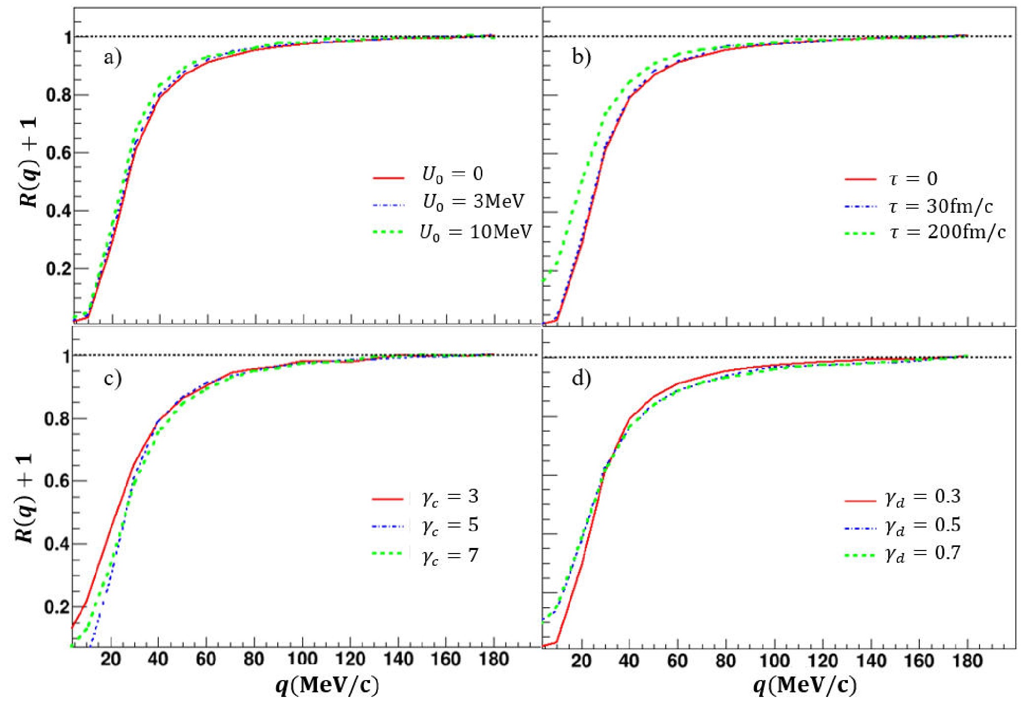
Figure 2. (color online) Influence of
$ \gamma_{{\rm{c}}} $ ,$ \gamma_{{\rm{d}}} $ ,$ U_0 $ , and τ on the correlation function of t-t pairs for the system, with all other parameters fixed at ($ E_{{\rm{b}}}=25 $ MeV/u,$ Z_{{\rm{p}}}=36 $ ,$ A_{{\rm{p}}}=86 $ ,$ Z_{{\rm{t}}}=82 $ ,$ A_{{\rm{t}}}=208 $ )$ \in {\cal{F}} $ . ($ \Delta t=1 $ fm/c,$ \gamma=0.5 $ ,$ t_{{\rm{max}}}=12000 $ fm/c,$ r_{{\rm{max}}}=500 $ fm)$ \in {\cal{C}} $ , with$ \sigma_{R}=4 $ fm and$ k_{\rm{B}}T=7.5 $ MeV. (a) Varying$ U_0 $ with fixed$ \gamma_{{\rm{c}}}=5 $ ,$ \gamma_d=0.3 $ , and$ \tau=0 $ . (b) Varying τ with fixed$ \gamma_{{\rm{c}}}=5 $ ,$ \gamma_d=0.3 $ , and$ U_0=0 $ . (c) Varying$ \gamma_{{\rm{c}}} $ with fixed$ \gamma_d=0.3 $ ,$ U_0=0 $ , and$ \tau=0 $ . (d) Varying$ \gamma_d $ with fixed$ \gamma_{{\rm{c}}}=5 $ ,$ U_0=0 $ , and$ \tau=0 $ . -
Up to this point, the full framework of the model has been presented. The correlation function between two particles emitted from the source can now be calculated numerically. This framework can be applied to experimental data for both pairs of intermediate mass fragments (IMFs) and pairs of light charged particles (LCPs).
Before applying the model to the experimental correlation functions, we first examine the effects of the main parameters on the correlation function. Figure 2 presents the triton-triton correlation functions for different parameter sets. In each panel, (a) to (d), only one parameter among
$ U_0 $ ,$ \gamma_c $ ,$ \gamma_d $ and τ is varied, while the others are fixed. The parameter$ U_0 $ denotes the potential well depth of the residual nucleus.$ \gamma_c $ denotes the ratio of the positive charge distribution size to the emission source size.$ \gamma_d $ is the ratio of the surface diffusion coefficient of the residual nucleus to the emission source size. τ is the characteristic emission time interval, equal to the reciprocal of the Poisson rate. Varying these four parameters within a reasonable range produces less pronounced changes in the correlation function than the influence of the emission source size$ \sigma_R $ (discussed below).
Figure 2. (color online) Influence of
$ \gamma_{{\rm{c}}} $ ,$ \gamma_{{\rm{d}}} $ ,$ U_0 $ , and τ on the correlation function of t-t pairs for the system, with all other parameters fixed at ($ E_{{\rm{b}}}=25 $ MeV/u,$ Z_{{\rm{p}}}=36 $ ,$ A_{{\rm{p}}}=86 $ ,$ Z_{{\rm{t}}}=82 $ ,$ A_{{\rm{t}}}=208 $ )$ \in {\cal{F}} $ . ($ \Delta t=1 $ fm/c,$ \gamma=0.5 $ ,$ t_{{\rm{max}}}=12000 $ fm/c,$ r_{{\rm{max}}}=500 $ fm)$ \in {\cal{C}} $ , with$ \sigma_{R}=4 $ fm and$ k_{\rm{B}}T=7.5 $ MeV. (a) Varying$ U_0 $ with fixed$ \gamma_{{\rm{c}}}=5 $ ,$ \gamma_d=0.3 $ , and$ \tau=0 $ . (b) Varying τ with fixed$ \gamma_{{\rm{c}}}=5 $ ,$ \gamma_d=0.3 $ , and$ U_0=0 $ . (c) Varying$ \gamma_{{\rm{c}}} $ with fixed$ \gamma_d=0.3 $ ,$ U_0=0 $ , and$ \tau=0 $ . (d) Varying$ \gamma_d $ with fixed$ \gamma_{{\rm{c}}}=5 $ ,$ U_0=0 $ , and$ \tau=0 $ . -
Up to this point, the full framework of the model has been presented. The correlation function between two particles emitted from the source can now be calculated numerically. This framework can be applied to experimental data for both pairs of intermediate mass fragments (IMFs) and pairs of light charged particles (LCPs).
Before applying the model to the experimental correlation functions, we first examine the effects of the main parameters on the correlation function. Figure 2 presents the triton-triton correlation functions for different parameter sets. In each panel, (a) to (d), only one parameter among
$ U_0 $ ,$ \gamma_c $ ,$ \gamma_d $ and τ is varied, while the others are fixed. The parameter$ U_0 $ denotes the potential well depth of the residual nucleus.$ \gamma_c $ denotes the ratio of the positive charge distribution size to the emission source size.$ \gamma_d $ is the ratio of the surface diffusion coefficient of the residual nucleus to the emission source size. τ is the characteristic emission time interval, equal to the reciprocal of the Poisson rate. Varying these four parameters within a reasonable range produces less pronounced changes in the correlation function than the influence of the emission source size$ \sigma_R $ (discussed below).
Figure 2. (color online) Influence of
$ \gamma_{{\rm{c}}} $ ,$ \gamma_{{\rm{d}}} $ ,$ U_0 $ , and τ on the correlation function of t-t pairs for the system, with all other parameters fixed at ($ E_{{\rm{b}}}=25 $ MeV/u,$ Z_{{\rm{p}}}=36 $ ,$ A_{{\rm{p}}}=86 $ ,$ Z_{{\rm{t}}}=82 $ ,$ A_{{\rm{t}}}=208 $ )$ \in {\cal{F}} $ . ($ \Delta t=1 $ fm/c,$ \gamma=0.5 $ ,$ t_{{\rm{max}}}=12000 $ fm/c,$ r_{{\rm{max}}}=500 $ fm)$ \in {\cal{C}} $ , with$ \sigma_{R}=4 $ fm and$ k_{\rm{B}}T=7.5 $ MeV. (a) Varying$ U_0 $ with fixed$ \gamma_{{\rm{c}}}=5 $ ,$ \gamma_d=0.3 $ , and$ \tau=0 $ . (b) Varying τ with fixed$ \gamma_{{\rm{c}}}=5 $ ,$ \gamma_d=0.3 $ , and$ U_0=0 $ . (c) Varying$ \gamma_{{\rm{c}}} $ with fixed$ \gamma_d=0.3 $ ,$ U_0=0 $ , and$ \tau=0 $ . (d) Varying$ \gamma_d $ with fixed$ \gamma_{{\rm{c}}}=5 $ ,$ U_0=0 $ , and$ \tau=0 $ . -
Up to this point, the full framework of the model has been presented. The correlation function between two particles emitted from the source can now be calculated numerically. This framework can be applied to experimental data for both pairs of intermediate mass fragments (IMFs) and pairs of light charged particles (LCPs).
Before applying the model to the experimental correlation functions, we first examine the effects of the main parameters on the correlation function. Figure 2 presents the triton-triton correlation functions for different parameter sets. In each panel, (a) to (d), only one parameter among
$ U_0 $ ,$ \gamma_c $ ,$ \gamma_d $ and τ is varied, while the others are fixed. The parameter$ U_0 $ denotes the potential well depth of the residual nucleus.$ \gamma_c $ denotes the ratio of the positive charge distribution size to the emission source size.$ \gamma_d $ is the ratio of the surface diffusion coefficient of the residual nucleus to the emission source size. τ is the characteristic emission time interval, equal to the reciprocal of the Poisson rate. Varying these four parameters within a reasonable range produces less pronounced changes in the correlation function than the influence of the emission source size$ \sigma_R $ (discussed below).
Figure 2. (color online) Influence of
$ \gamma_{{\rm{c}}} $ ,$ \gamma_{{\rm{d}}} $ ,$ U_0 $ , and τ on the correlation function of t-t pairs for the system, with all other parameters fixed at ($ E_{{\rm{b}}}=25 $ MeV/u,$ Z_{{\rm{p}}}=36 $ ,$ A_{{\rm{p}}}=86 $ ,$ Z_{{\rm{t}}}=82 $ ,$ A_{{\rm{t}}}=208 $ )$ \in {\cal{F}} $ . ($ \Delta t=1 $ fm/c,$ \gamma=0.5 $ ,$ t_{{\rm{max}}}=12000 $ fm/c,$ r_{{\rm{max}}}=500 $ fm)$ \in {\cal{C}} $ , with$ \sigma_{R}=4 $ fm and$ k_{\rm{B}}T=7.5 $ MeV. (a) Varying$ U_0 $ with fixed$ \gamma_{{\rm{c}}}=5 $ ,$ \gamma_d=0.3 $ , and$ \tau=0 $ . (b) Varying τ with fixed$ \gamma_{{\rm{c}}}=5 $ ,$ \gamma_d=0.3 $ , and$ U_0=0 $ . (c) Varying$ \gamma_{{\rm{c}}} $ with fixed$ \gamma_d=0.3 $ ,$ U_0=0 $ , and$ \tau=0 $ . (d) Varying$ \gamma_d $ with fixed$ \gamma_{{\rm{c}}}=5 $ ,$ U_0=0 $ , and$ \tau=0 $ . -
Up to this point, the full framework of the model has been presented. The correlation function between two particles emitted from the source can now be calculated numerically. This framework can be applied to experimental data for both pairs of intermediate mass fragments (IMFs) and pairs of light charged particles (LCPs).
Before applying the model to the experimental correlation functions, we first examine the effects of the main parameters on the correlation function. Figure 2 presents the triton-triton correlation functions for different parameter sets. In each panel, (a) to (d), only one parameter among
$ U_0 $ ,$ \gamma_c $ ,$ \gamma_d $ and τ is varied, while the others are fixed. The parameter$ U_0 $ denotes the potential well depth of the residual nucleus.$ \gamma_c $ denotes the ratio of the positive charge distribution size to the emission source size.$ \gamma_d $ is the ratio of the surface diffusion coefficient of the residual nucleus to the emission source size. τ is the characteristic emission time interval, equal to the reciprocal of the Poisson rate. Varying these four parameters within a reasonable range produces less pronounced changes in the correlation function than the influence of the emission source size$ \sigma_R $ (discussed below).
Figure 2. (color online) Influence of
$ \gamma_{{\rm{c}}} $ ,$ \gamma_{{\rm{d}}} $ ,$ U_0 $ , and τ on the correlation function of t-t pairs for the system, with all other parameters fixed at ($ E_{{\rm{b}}}=25 $ MeV/u,$ Z_{{\rm{p}}}=36 $ ,$ A_{{\rm{p}}}=86 $ ,$ Z_{{\rm{t}}}=82 $ ,$ A_{{\rm{t}}}=208 $ )$ \in {\cal{F}} $ . ($ \Delta t=1 $ fm/c,$ \gamma=0.5 $ ,$ t_{{\rm{max}}}=12000 $ fm/c,$ r_{{\rm{max}}}=500 $ fm)$ \in {\cal{C}} $ , with$ \sigma_{R}=4 $ fm and$ k_{\rm{B}}T=7.5 $ MeV. (a) Varying$ U_0 $ with fixed$ \gamma_{{\rm{c}}}=5 $ ,$ \gamma_d=0.3 $ , and$ \tau=0 $ . (b) Varying τ with fixed$ \gamma_{{\rm{c}}}=5 $ ,$ \gamma_d=0.3 $ , and$ U_0=0 $ . (c) Varying$ \gamma_{{\rm{c}}} $ with fixed$ \gamma_d=0.3 $ ,$ U_0=0 $ , and$ \tau=0 $ . (d) Varying$ \gamma_d $ with fixed$ \gamma_{{\rm{c}}}=5 $ ,$ U_0=0 $ , and$ \tau=0 $ . -
We first apply the model to calculate the correlation functions of IMF pairs. The abundant IMFs emitted in Fermi-energy HIRs carry crucial information about the violent reaction dynamics during the early stages. For instance, the correlation function of IMFs provides insights into the IMF emission timescale, which depends on the isospin of the reaction systems [36], as well as the space-time evolution of the colliding system [37–38]. The experimental data are taken from approximately central Ar+Au reactions at a beam energy of 35 MeV/u, with charged particles measured by the Miniball at Michigan State University [39]. The correlation function is constructed using IMF detectors in Ring 2 and Ring 3, located at polar angles of
$ \theta_{{\rm{lab}}}=19.5^\circ $ and$ \theta_{{\rm{lab}}}=27^\circ $ , respectively. For details of the experiment, see Ref. [39].For the interaction between the two correlated IMFs, it is reasonable to consider only the long-range Coulomb interaction. The mean field of the emitting source, including both Coulomb and nuclear potentials, is taken into account. Figure 3 presents the correlation function for Boron isotopes. Since the masses are not resolved, we set
$ A_1=A_2=10 $ for the calculation. For a rough comparison, we omit the detector-filtering procedure because the efficiency loss is largely canceled when taking the ratio of the relative momentum spectrum in the same event to that in the mixed event, as shown in Eq. (40).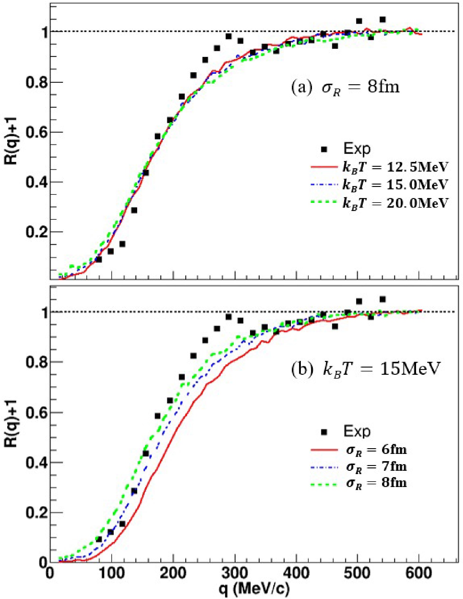
Figure 3. (color online) Correlation functions of B-B pairs compared with the CTA-Ⅰ model predictions for the 36Ar + 197Au reaction at
$ E/A=35 $ MeV/u. (a) Varying$ k_BT $ with fixed$ \sigma_R=8 $ fm. (b) Varying$ \sigma_R $ with fixed$ k_BT=15 $ MeV. Data points were extracted from [39]; the statistical uncertainties are comparable to the symbol size.Figure 3 (a) compares the calculations with a fixed source size of
$ \sigma_{{\rm{R}}}= 8 $ fm, while the temperature$ k_{{\rm{B}}}T $ varies from 10 to 20 MeV. As expected, the correlation function shows negligible dependence on the temperature parameter. By contrast, Fig. 3 (b) shows the results for a fixed$ k_{{\rm{B}}}T=15 $ MeV, with the source size$ \sigma_{{\rm{R}}} $ varied from 6 to 8 fm. Although the variation in the source size is only 1 fm, it has a substantial effect. The correlation becomes noticeably stronger when the source size decreases by 1 fm. With the parameters set to$ k_{{\rm{B}}}T=15 $ MeV and$ \sigma_{{\rm{R}}}= 8 $ fm, the experimental trend is well reproduced. These parameters are consistent with those extracted in Ref. [39]. Notably, the small peak structure around$ q \approx 300 $ MeV/c is not accounted for in this model, as it is unlikely to have a real physical origin. -
We first apply the model to calculate the correlation functions of IMF pairs. The abundant IMFs emitted in Fermi-energy HIRs carry crucial information about the violent reaction dynamics during the early stages. For instance, the correlation function of IMFs provides insights into the IMF emission timescale, which depends on the isospin of the reaction systems [36], as well as the space-time evolution of the colliding system [37–38]. The experimental data are taken from approximately central Ar+Au reactions at a beam energy of 35 MeV/u, with charged particles measured by the Miniball at Michigan State University [39]. The correlation function is constructed using IMF detectors in Ring 2 and Ring 3, located at polar angles of
$ \theta_{{\rm{lab}}}=19.5^\circ $ and$ \theta_{{\rm{lab}}}=27^\circ $ , respectively. For details of the experiment, see Ref. [39].For the interaction between the two correlated IMFs, it is reasonable to consider only the long-range Coulomb interaction. The mean field of the emitting source, including both Coulomb and nuclear potentials, is taken into account. Figure 3 presents the correlation function for Boron isotopes. Since the masses are not resolved, we set
$ A_1=A_2=10 $ for the calculation. For a rough comparison, we omit the detector-filtering procedure because the efficiency loss is largely canceled when taking the ratio of the relative momentum spectrum in the same event to that in the mixed event, as shown in Eq. (40).
Figure 3. (color online) Correlation functions of B-B pairs compared with the CTA-Ⅰ model predictions for the 36Ar + 197Au reaction at
$ E/A=35 $ MeV/u. (a) Varying$ k_BT $ with fixed$ \sigma_R=8 $ fm. (b) Varying$ \sigma_R $ with fixed$ k_BT=15 $ MeV. Data points were extracted from [39]; the statistical uncertainties are comparable to the symbol size.Figure 3 (a) compares the calculations with a fixed source size of
$ \sigma_{{\rm{R}}}= 8 $ fm, while the temperature$ k_{{\rm{B}}}T $ varies from 10 to 20 MeV. As expected, the correlation function shows negligible dependence on the temperature parameter. By contrast, Fig. 3 (b) shows the results for a fixed$ k_{{\rm{B}}}T=15 $ MeV, with the source size$ \sigma_{{\rm{R}}} $ varied from 6 to 8 fm. Although the variation in the source size is only 1 fm, it has a substantial effect. The correlation becomes noticeably stronger when the source size decreases by 1 fm. With the parameters set to$ k_{{\rm{B}}}T=15 $ MeV and$ \sigma_{{\rm{R}}}= 8 $ fm, the experimental trend is well reproduced. These parameters are consistent with those extracted in Ref. [39]. Notably, the small peak structure around$ q \approx 300 $ MeV/c is not accounted for in this model, as it is unlikely to have a real physical origin. -
We first apply the model to calculate the correlation functions of IMF pairs. The abundant IMFs emitted in Fermi-energy HIRs carry crucial information about the violent reaction dynamics during the early stages. For instance, the correlation function of IMFs provides insights into the IMF emission timescale, which depends on the isospin of the reaction systems [36], as well as the space-time evolution of the colliding system [37–38]. The experimental data are taken from approximately central Ar+Au reactions at a beam energy of 35 MeV/u, with charged particles measured by the Miniball at Michigan State University [39]. The correlation function is constructed using IMF detectors in Ring 2 and Ring 3, located at polar angles of
$ \theta_{{\rm{lab}}}=19.5^\circ $ and$ \theta_{{\rm{lab}}}=27^\circ $ , respectively. For details of the experiment, see Ref. [39].For the interaction between the two correlated IMFs, it is reasonable to consider only the long-range Coulomb interaction. The mean field of the emitting source, including both Coulomb and nuclear potentials, is taken into account. Figure 3 presents the correlation function for Boron isotopes. Since the masses are not resolved, we set
$ A_1=A_2=10 $ for the calculation. For a rough comparison, we omit the detector-filtering procedure because the efficiency loss is largely canceled when taking the ratio of the relative momentum spectrum in the same event to that in the mixed event, as shown in Eq. (40).
Figure 3. (color online) Correlation functions of B-B pairs compared with the CTA-Ⅰ model predictions for the 36Ar + 197Au reaction at
$ E/A=35 $ MeV/u. (a) Varying$ k_BT $ with fixed$ \sigma_R=8 $ fm. (b) Varying$ \sigma_R $ with fixed$ k_BT=15 $ MeV. Data points were extracted from [39]; the statistical uncertainties are comparable to the symbol size.Figure 3 (a) compares the calculations with a fixed source size of
$ \sigma_{{\rm{R}}}= 8 $ fm, while the temperature$ k_{{\rm{B}}}T $ varies from 10 to 20 MeV. As expected, the correlation function shows negligible dependence on the temperature parameter. By contrast, Fig. 3 (b) shows the results for a fixed$ k_{{\rm{B}}}T=15 $ MeV, with the source size$ \sigma_{{\rm{R}}} $ varied from 6 to 8 fm. Although the variation in the source size is only 1 fm, it has a substantial effect. The correlation becomes noticeably stronger when the source size decreases by 1 fm. With the parameters set to$ k_{{\rm{B}}}T=15 $ MeV and$ \sigma_{{\rm{R}}}= 8 $ fm, the experimental trend is well reproduced. These parameters are consistent with those extracted in Ref. [39]. Notably, the small peak structure around$ q \approx 300 $ MeV/c is not accounted for in this model, as it is unlikely to have a real physical origin. -
We first apply the model to calculate the correlation functions of IMF pairs. The abundant IMFs emitted in Fermi-energy HIRs carry crucial information about the violent reaction dynamics during the early stages. For instance, the correlation function of IMFs provides insights into the IMF emission timescale, which depends on the isospin of the reaction systems [36], as well as the space-time evolution of the colliding system [37–38]. The experimental data are taken from approximately central Ar+Au reactions at a beam energy of 35 MeV/u, with charged particles measured by the Miniball at Michigan State University [39]. The correlation function is constructed using IMF detectors in Ring 2 and Ring 3, located at polar angles of
$ \theta_{{\rm{lab}}}=19.5^\circ $ and$ \theta_{{\rm{lab}}}=27^\circ $ , respectively. For details of the experiment, see Ref. [39].For the interaction between the two correlated IMFs, it is reasonable to consider only the long-range Coulomb interaction. The mean field of the emitting source, including both Coulomb and nuclear potentials, is taken into account. Figure 3 presents the correlation function for Boron isotopes. Since the masses are not resolved, we set
$ A_1=A_2=10 $ for the calculation. For a rough comparison, we omit the detector-filtering procedure because the efficiency loss is largely canceled when taking the ratio of the relative momentum spectrum in the same event to that in the mixed event, as shown in Eq. (40).
Figure 3. (color online) Correlation functions of B-B pairs compared with the CTA-Ⅰ model predictions for the 36Ar + 197Au reaction at
$ E/A=35 $ MeV/u. (a) Varying$ k_BT $ with fixed$ \sigma_R=8 $ fm. (b) Varying$ \sigma_R $ with fixed$ k_BT=15 $ MeV. Data points were extracted from [39]; the statistical uncertainties are comparable to the symbol size.Figure 3 (a) compares the calculations with a fixed source size of
$ \sigma_{{\rm{R}}}= 8 $ fm, while the temperature$ k_{{\rm{B}}}T $ varies from 10 to 20 MeV. As expected, the correlation function shows negligible dependence on the temperature parameter. By contrast, Fig. 3 (b) shows the results for a fixed$ k_{{\rm{B}}}T=15 $ MeV, with the source size$ \sigma_{{\rm{R}}} $ varied from 6 to 8 fm. Although the variation in the source size is only 1 fm, it has a substantial effect. The correlation becomes noticeably stronger when the source size decreases by 1 fm. With the parameters set to$ k_{{\rm{B}}}T=15 $ MeV and$ \sigma_{{\rm{R}}}= 8 $ fm, the experimental trend is well reproduced. These parameters are consistent with those extracted in Ref. [39]. Notably, the small peak structure around$ q \approx 300 $ MeV/c is not accounted for in this model, as it is unlikely to have a real physical origin. -
We first apply the model to calculate the correlation functions of IMF pairs. The abundant IMFs emitted in Fermi-energy HIRs carry crucial information about the violent reaction dynamics during the early stages. For instance, the correlation function of IMFs provides insights into the IMF emission timescale, which depends on the isospin of the reaction systems [36], as well as the space-time evolution of the colliding system [37–38]. The experimental data are taken from approximately central Ar+Au reactions at a beam energy of 35 MeV/u, with charged particles measured by the Miniball at Michigan State University [39]. The correlation function is constructed using IMF detectors in Ring 2 and Ring 3, located at polar angles of
$ \theta_{{\rm{lab}}}=19.5^\circ $ and$ \theta_{{\rm{lab}}}=27^\circ $ , respectively. For details of the experiment, see Ref. [39].For the interaction between the two correlated IMFs, it is reasonable to consider only the long-range Coulomb interaction. The mean field of the emitting source, including both Coulomb and nuclear potentials, is taken into account. Figure 3 presents the correlation function for Boron isotopes. Since the masses are not resolved, we set
$ A_1=A_2=10 $ for the calculation. For a rough comparison, we omit the detector-filtering procedure because the efficiency loss is largely canceled when taking the ratio of the relative momentum spectrum in the same event to that in the mixed event, as shown in Eq. (40).
Figure 3. (color online) Correlation functions of B-B pairs compared with the CTA-Ⅰ model predictions for the 36Ar + 197Au reaction at
$ E/A=35 $ MeV/u. (a) Varying$ k_BT $ with fixed$ \sigma_R=8 $ fm. (b) Varying$ \sigma_R $ with fixed$ k_BT=15 $ MeV. Data points were extracted from [39]; the statistical uncertainties are comparable to the symbol size.Figure 3 (a) compares the calculations with a fixed source size of
$ \sigma_{{\rm{R}}}= 8 $ fm, while the temperature$ k_{{\rm{B}}}T $ varies from 10 to 20 MeV. As expected, the correlation function shows negligible dependence on the temperature parameter. By contrast, Fig. 3 (b) shows the results for a fixed$ k_{{\rm{B}}}T=15 $ MeV, with the source size$ \sigma_{{\rm{R}}} $ varied from 6 to 8 fm. Although the variation in the source size is only 1 fm, it has a substantial effect. The correlation becomes noticeably stronger when the source size decreases by 1 fm. With the parameters set to$ k_{{\rm{B}}}T=15 $ MeV and$ \sigma_{{\rm{R}}}= 8 $ fm, the experimental trend is well reproduced. These parameters are consistent with those extracted in Ref. [39]. Notably, the small peak structure around$ q \approx 300 $ MeV/c is not accounted for in this model, as it is unlikely to have a real physical origin. -
Finally, the model is applied to interpret the correlation function of an LCP pair. The proton-proton (p-p) correlation function is not considered here because the positive correlation peak associated with s-wave p-p resonant scattering cannot be reliably treated within a classical framework. Instead, we examine triton-triton (t-t) and 3He-3He pairs. The data were obtained from the 25 MeV/u 86Kr+natPb reaction measured with the compact spectrometer for heavy ion experiment (CSHINE) [40], which is installed at the final focal plane of the radioactive ion beam line at Lanzhou (RIBLL). The charged particles were detected by four silicon strip detector (SSD) telescopes, each consisting of a single-sided SSD, a double-sided SSD, and a
$ 3\times 3 $ CsI(Tl) array. The pixel size of each telescope is$ 4\, {\mathrm{mm}} \times4 \, {\mathrm{mm }}$ , ensuring high position resolution. The energy resolution is better than 2% [41]. A track-finding algorithm has been developed to identify the complicated firing patterns in the SSD telescopes [42–43]. Three parallel plate avalanche counters (PPACs) were mounted to detect the fission fragments and reconstruct the event geometry. However, for the correlation-function analysis presented here, no event-geometry selection is applied because of the low statistics of four-body coincidence events. Details of the experimental setup can be found in Refs. [42−45].Figure 4 presents the correlation functions of the t-t pair in comparison with the model calculations. The mean
$ R_{{\rm{LMT}}} $ value is set to 0.8 in this analysis. As an example, the parameter settings are listed as follows. ($ E_{{\rm{b}}}=25 $ MeV/u,$ Z_{{\rm{p}}}=36 $ ,$ A_{{\rm{p}}}=86 $ ,$ Z_{{\rm{t}}}=82 $ ,$ A_{{\rm{t}}}=208 $ )$ \in {\cal{F}} $ . ($ \Delta t=1 $ fm/c,$ \gamma=0.5 $ ,$ t_{{\rm{max}}}=12000 $ fm/c,$ r_{{\rm{max}}}=500 $ fm)$ \in {\cal{C}} $ .$ \gamma_{{\rm{c}}}=5 $ ,$ \gamma_d=0.3 $ ,$ U_0=0 $ . Panels (a) and (b) present the calculations obtained by varying$ k_{{\rm{B}}}T $ and$ \sigma_{{\rm{R}}} $ , respectively. In panel (a), the source size parameter is fixed at$ \sigma_{{\rm{R}}}=4 $ fm. Again, the parameter$ k_{{\rm{B}}}T $ has only a weak impact on the correlation function. In panel (b), where$ k_{{\rm{B}}}T=7.5 $ MeV is fixed, the correlation function exhibits a strong dependence on the source size parameter$ \sigma_{{\rm{R}}} $ , consistent with the picture that the correlation function can be used to probe the spatiotemporal size of the source. We note that the temperature parameter for tritons is much lower than that for boron in Fig. 3 because, in a qualitative picture, triton emission persists to a relatively later stage due to its much lower Coulomb barrier.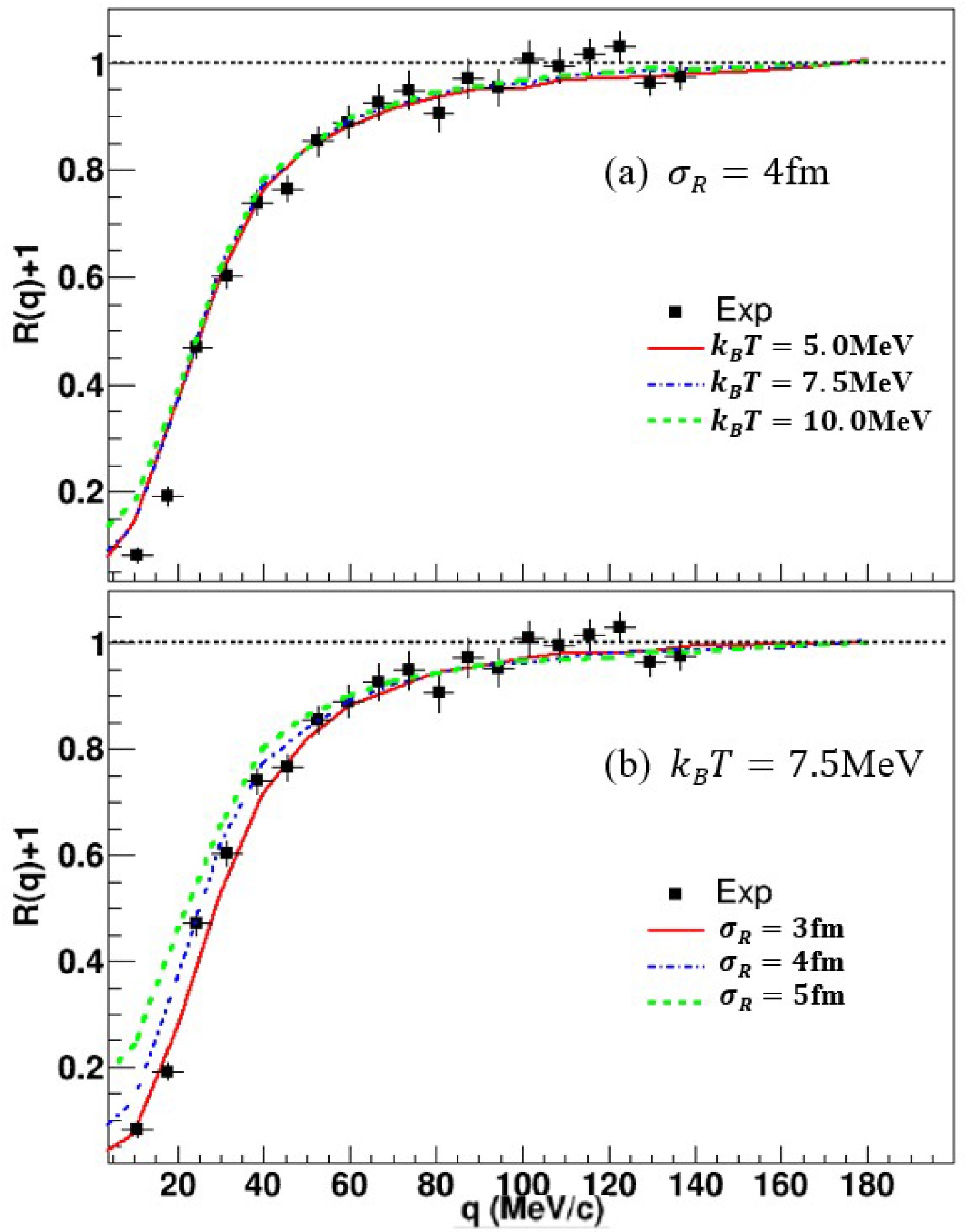
Figure 4. (color online) Correlation function for triton–triton pairs in 25 MeV/u 86Kr+natPb reactions compared with the CTA-Ⅰ model predictions. The statistical uncertainties of the data points are indicated. (a) Varying
$ k_BT $ with fixed$ \sigma_R=4 $ fm. (b) Varying$ \sigma_R $ with fixed$ k_BT=7.5 $ MeV.Figure 5 shows the calculated 3He-3He correlation functions together with the experimental data points. Because the reaction system is neutron-rich, the 3He yield is low; consequently, the 3He-pair correlation function suffers from limited statistics. Nevertheless, the theoretical curves show similar trends as
$ k_{{\rm{B}}}T $ and$ \sigma_{{\rm{R}}} $ are varied. Specifically, varying$ k_{{\rm{B}}}T $ within a reasonable range has a smaller effect on the correlation than varying the source-size parameter$ \sigma_{{\rm{R}}} $ . Despite the large fluctuations in the data points, the experimental trend is consistent with the calculation using$ k_{{\rm{B}}}T=10.0 $ MeV and$ \sigma_R=6 $ fm, and the source-size dependence is more pronounced than the temperature dependence.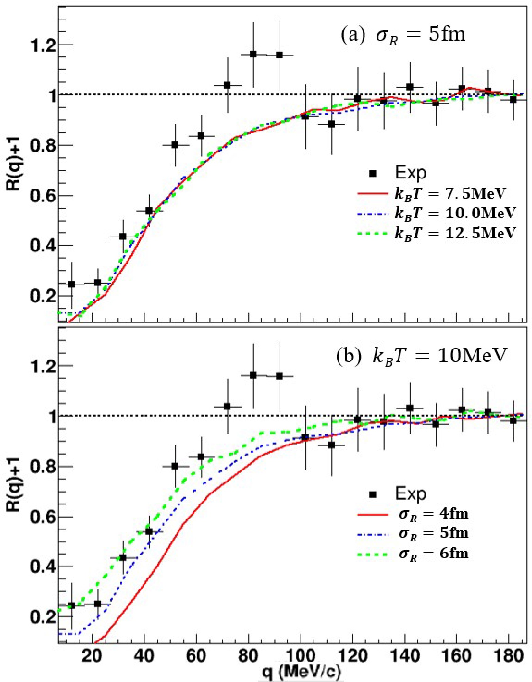
Figure 5. (color online) Correlation function for
$ ^{3}{\mathrm{He}} \text- ^{3}{\mathrm{He}} $ pairs in 25 MeV/u 86Kr+natPb reactions, compared with CTA-Ⅰ model predictions. (a) Variation with$ k_BT $ at fixed$ \sigma_R=5 $ fm. (b) Variation with$ \sigma_R $ at fixed$ k_BT=10 $ MeV.The model calculation reveals subtle differences between the t-t and 3He-3He correlation functions. Comparing the model predictions in Fig. 5 (b) and Fig. 4 (b) for the same reaction system shows that the change in the correlation function is more pronounced for the 3He-3He pair than for the t-t pair when
$ \sigma_{{\rm{R}}} $ is varied by the same amount of 1 fm. This is because the anticorrelation arising from the Coulomb interaction is much stronger in the former. Although the model–data comparison suggests different emission sizes for tritons and 3He, the large experimental uncertainty prevents us from extracting the isospin effect of the source parameter here. Nevertheless, reasonably high-quality correlation function data for t-t and 3He-3He pairs could potentially be used to probe the isospin effect of particle emission from the HIR process.It is worth mentioning that the current version of our model successfully reproduces the experimental correlation functions in various systems based solely on simple assumptions, namely the Poisson process and thermal equilibrium. This demonstrates the feasibility of the model for describing the emission source in heavy-ion reactions from a statistical perspective. In principle, the model can be extended to accommodate a variety of scenarios by incorporating more realistic descriptions of the experimental conditions. For instance:
i) The spherical assumption can be relaxed, allowing the source to have non-spherical geometries such as disks or rings. This extension allows the source to behave as a rotating system while still maintaining the assumption of thermal equilibrium. Such a situation may occur in fast-fission events in heavy-ion reactions [45–46]. In this case, analyzing the correlation functions (CFs) as a function of the direction of the relative momentum would be of interest.
ii) If the emission rate is sufficiently high to drive the emission process from a Poisson process to a Gaussian process, the thermal equilibrium assumption will break down. In this non-equilibrium regime, the process can be treated within the relaxation time approximation, where the relaxation time is explicitly linked to the effective emission rate of the Gaussian process. Research on extending the current model to such situations is ongoing.
-
Finally, the model is applied to interpret the correlation function of an LCP pair. The proton-proton (p-p) correlation function is not considered here because the positive correlation peak associated with s-wave p-p resonant scattering cannot be reliably treated within a classical framework. Instead, we examine triton-triton (t-t) and 3He-3He pairs. The data were obtained from the 25 MeV/u 86Kr+natPb reaction measured with the compact spectrometer for heavy ion experiment (CSHINE) [40], which is installed at the final focal plane of the radioactive ion beam line at Lanzhou (RIBLL). The charged particles were detected by four silicon strip detector (SSD) telescopes, each consisting of a single-sided SSD, a double-sided SSD, and a
$ 3\times 3 $ CsI(Tl) array. The pixel size of each telescope is$ 4\, {\mathrm{mm}} \times4 \, {\mathrm{mm }}$ , ensuring high position resolution. The energy resolution is better than 2% [41]. A track-finding algorithm has been developed to identify the complicated firing patterns in the SSD telescopes [42–43]. Three parallel plate avalanche counters (PPACs) were mounted to detect the fission fragments and reconstruct the event geometry. However, for the correlation-function analysis presented here, no event-geometry selection is applied because of the low statistics of four-body coincidence events. Details of the experimental setup can be found in Refs. [42−45].Figure 4 presents the correlation functions of the t-t pair in comparison with the model calculations. The mean
$ R_{{\rm{LMT}}} $ value is set to 0.8 in this analysis. As an example, the parameter settings are listed as follows. ($ E_{{\rm{b}}}=25 $ MeV/u,$ Z_{{\rm{p}}}=36 $ ,$ A_{{\rm{p}}}=86 $ ,$ Z_{{\rm{t}}}=82 $ ,$ A_{{\rm{t}}}=208 $ )$ \in {\cal{F}} $ . ($ \Delta t=1 $ fm/c,$ \gamma=0.5 $ ,$ t_{{\rm{max}}}=12000 $ fm/c,$ r_{{\rm{max}}}=500 $ fm)$ \in {\cal{C}} $ .$ \gamma_{{\rm{c}}}=5 $ ,$ \gamma_d=0.3 $ ,$ U_0=0 $ . Panels (a) and (b) present the calculations obtained by varying$ k_{{\rm{B}}}T $ and$ \sigma_{{\rm{R}}} $ , respectively. In panel (a), the source size parameter is fixed at$ \sigma_{{\rm{R}}}=4 $ fm. Again, the parameter$ k_{{\rm{B}}}T $ has only a weak impact on the correlation function. In panel (b), where$ k_{{\rm{B}}}T=7.5 $ MeV is fixed, the correlation function exhibits a strong dependence on the source size parameter$ \sigma_{{\rm{R}}} $ , consistent with the picture that the correlation function can be used to probe the spatiotemporal size of the source. We note that the temperature parameter for tritons is much lower than that for boron in Fig. 3 because, in a qualitative picture, triton emission persists to a relatively later stage due to its much lower Coulomb barrier.
Figure 4. (color online) Correlation function for triton–triton pairs in 25 MeV/u 86Kr+natPb reactions compared with the CTA-Ⅰ model predictions. The statistical uncertainties of the data points are indicated. (a) Varying
$ k_BT $ with fixed$ \sigma_R=4 $ fm. (b) Varying$ \sigma_R $ with fixed$ k_BT=7.5 $ MeV.Figure 5 shows the calculated 3He-3He correlation functions together with the experimental data points. Because the reaction system is neutron-rich, the 3He yield is low; consequently, the 3He-pair correlation function suffers from limited statistics. Nevertheless, the theoretical curves show similar trends as
$ k_{{\rm{B}}}T $ and$ \sigma_{{\rm{R}}} $ are varied. Specifically, varying$ k_{{\rm{B}}}T $ within a reasonable range has a smaller effect on the correlation than varying the source-size parameter$ \sigma_{{\rm{R}}} $ . Despite the large fluctuations in the data points, the experimental trend is consistent with the calculation using$ k_{{\rm{B}}}T=10.0 $ MeV and$ \sigma_R=6 $ fm, and the source-size dependence is more pronounced than the temperature dependence.
Figure 5. (color online) Correlation function for
$ ^{3}{\mathrm{He}} \text- ^{3}{\mathrm{He}} $ pairs in 25 MeV/u 86Kr+natPb reactions, compared with CTA-Ⅰ model predictions. (a) Variation with$ k_BT $ at fixed$ \sigma_R=5 $ fm. (b) Variation with$ \sigma_R $ at fixed$ k_BT=10 $ MeV.The model calculation reveals subtle differences between the t-t and 3He-3He correlation functions. Comparing the model predictions in Fig. 5 (b) and Fig. 4 (b) for the same reaction system shows that the change in the correlation function is more pronounced for the 3He-3He pair than for the t-t pair when
$ \sigma_{{\rm{R}}} $ is varied by the same amount of 1 fm. This is because the anticorrelation arising from the Coulomb interaction is much stronger in the former. Although the model–data comparison suggests different emission sizes for tritons and 3He, the large experimental uncertainty prevents us from extracting the isospin effect of the source parameter here. Nevertheless, reasonably high-quality correlation function data for t-t and 3He-3He pairs could potentially be used to probe the isospin effect of particle emission from the HIR process.It is worth mentioning that the current version of our model successfully reproduces the experimental correlation functions in various systems based solely on simple assumptions, namely the Poisson process and thermal equilibrium. This demonstrates the feasibility of the model for describing the emission source in heavy-ion reactions from a statistical perspective. In principle, the model can be extended to accommodate a variety of scenarios by incorporating more realistic descriptions of the experimental conditions. For instance:
i) The spherical assumption can be relaxed, allowing the source to have non-spherical geometries such as disks or rings. This extension allows the source to behave as a rotating system while still maintaining the assumption of thermal equilibrium. Such a situation may occur in fast-fission events in heavy-ion reactions [45–46]. In this case, analyzing the correlation functions (CFs) as a function of the direction of the relative momentum would be of interest.
ii) If the emission rate is sufficiently high to drive the emission process from a Poisson process to a Gaussian process, the thermal equilibrium assumption will break down. In this non-equilibrium regime, the process can be treated within the relaxation time approximation, where the relaxation time is explicitly linked to the effective emission rate of the Gaussian process. Research on extending the current model to such situations is ongoing.
-
Finally, the model is applied to interpret the correlation function of an LCP pair. The proton-proton (p-p) correlation function is not considered here because the positive correlation peak associated with s-wave p-p resonant scattering cannot be reliably treated within a classical framework. Instead, we examine triton-triton (t-t) and 3He-3He pairs. The data were obtained from the 25 MeV/u 86Kr+natPb reaction measured with the compact spectrometer for heavy ion experiment (CSHINE) [40], which is installed at the final focal plane of the radioactive ion beam line at Lanzhou (RIBLL). The charged particles were detected by four silicon strip detector (SSD) telescopes, each consisting of a single-sided SSD, a double-sided SSD, and a
$ 3\times 3 $ CsI(Tl) array. The pixel size of each telescope is$ 4\, {\mathrm{mm}} \times4 \, {\mathrm{mm }}$ , ensuring high position resolution. The energy resolution is better than 2% [41]. A track-finding algorithm has been developed to identify the complicated firing patterns in the SSD telescopes [42–43]. Three parallel plate avalanche counters (PPACs) were mounted to detect the fission fragments and reconstruct the event geometry. However, for the correlation-function analysis presented here, no event-geometry selection is applied because of the low statistics of four-body coincidence events. Details of the experimental setup can be found in Refs. [42−45].Figure 4 presents the correlation functions of the t-t pair in comparison with the model calculations. The mean
$ R_{{\rm{LMT}}} $ value is set to 0.8 in this analysis. As an example, the parameter settings are listed as follows. ($ E_{{\rm{b}}}=25 $ MeV/u,$ Z_{{\rm{p}}}=36 $ ,$ A_{{\rm{p}}}=86 $ ,$ Z_{{\rm{t}}}=82 $ ,$ A_{{\rm{t}}}=208 $ )$ \in {\cal{F}} $ . ($ \Delta t=1 $ fm/c,$ \gamma=0.5 $ ,$ t_{{\rm{max}}}=12000 $ fm/c,$ r_{{\rm{max}}}=500 $ fm)$ \in {\cal{C}} $ .$ \gamma_{{\rm{c}}}=5 $ ,$ \gamma_d=0.3 $ ,$ U_0=0 $ . Panels (a) and (b) present the calculations obtained by varying$ k_{{\rm{B}}}T $ and$ \sigma_{{\rm{R}}} $ , respectively. In panel (a), the source size parameter is fixed at$ \sigma_{{\rm{R}}}=4 $ fm. Again, the parameter$ k_{{\rm{B}}}T $ has only a weak impact on the correlation function. In panel (b), where$ k_{{\rm{B}}}T=7.5 $ MeV is fixed, the correlation function exhibits a strong dependence on the source size parameter$ \sigma_{{\rm{R}}} $ , consistent with the picture that the correlation function can be used to probe the spatiotemporal size of the source. We note that the temperature parameter for tritons is much lower than that for boron in Fig. 3 because, in a qualitative picture, triton emission persists to a relatively later stage due to its much lower Coulomb barrier.
Figure 4. (color online) Correlation function for triton–triton pairs in 25 MeV/u 86Kr+natPb reactions compared with the CTA-Ⅰ model predictions. The statistical uncertainties of the data points are indicated. (a) Varying
$ k_BT $ with fixed$ \sigma_R=4 $ fm. (b) Varying$ \sigma_R $ with fixed$ k_BT=7.5 $ MeV.Figure 5 shows the calculated 3He-3He correlation functions together with the experimental data points. Because the reaction system is neutron-rich, the 3He yield is low; consequently, the 3He-pair correlation function suffers from limited statistics. Nevertheless, the theoretical curves show similar trends as
$ k_{{\rm{B}}}T $ and$ \sigma_{{\rm{R}}} $ are varied. Specifically, varying$ k_{{\rm{B}}}T $ within a reasonable range has a smaller effect on the correlation than varying the source-size parameter$ \sigma_{{\rm{R}}} $ . Despite the large fluctuations in the data points, the experimental trend is consistent with the calculation using$ k_{{\rm{B}}}T=10.0 $ MeV and$ \sigma_R=6 $ fm, and the source-size dependence is more pronounced than the temperature dependence.
Figure 5. (color online) Correlation function for
$ ^{3}{\mathrm{He}} \text- ^{3}{\mathrm{He}} $ pairs in 25 MeV/u 86Kr+natPb reactions, compared with CTA-Ⅰ model predictions. (a) Variation with$ k_BT $ at fixed$ \sigma_R=5 $ fm. (b) Variation with$ \sigma_R $ at fixed$ k_BT=10 $ MeV.The model calculation reveals subtle differences between the t-t and 3He-3He correlation functions. Comparing the model predictions in Fig. 5 (b) and Fig. 4 (b) for the same reaction system shows that the change in the correlation function is more pronounced for the 3He-3He pair than for the t-t pair when
$ \sigma_{{\rm{R}}} $ is varied by the same amount of 1 fm. This is because the anticorrelation arising from the Coulomb interaction is much stronger in the former. Although the model–data comparison suggests different emission sizes for tritons and 3He, the large experimental uncertainty prevents us from extracting the isospin effect of the source parameter here. Nevertheless, reasonably high-quality correlation function data for t-t and 3He-3He pairs could potentially be used to probe the isospin effect of particle emission from the HIR process.It is worth mentioning that the current version of our model successfully reproduces the experimental correlation functions in various systems based solely on simple assumptions, namely the Poisson process and thermal equilibrium. This demonstrates the feasibility of the model for describing the emission source in heavy-ion reactions from a statistical perspective. In principle, the model can be extended to accommodate a variety of scenarios by incorporating more realistic descriptions of the experimental conditions. For instance:
i) The spherical assumption can be relaxed, allowing the source to have non-spherical geometries such as disks or rings. This extension allows the source to behave as a rotating system while still maintaining the assumption of thermal equilibrium. Such a situation may occur in fast-fission events in heavy-ion reactions [45–46]. In this case, analyzing the correlation functions (CFs) as a function of the direction of the relative momentum would be of interest.
ii) If the emission rate is sufficiently high to drive the emission process from a Poisson process to a Gaussian process, the thermal equilibrium assumption will break down. In this non-equilibrium regime, the process can be treated within the relaxation time approximation, where the relaxation time is explicitly linked to the effective emission rate of the Gaussian process. Research on extending the current model to such situations is ongoing.
-
Finally, the model is applied to interpret the correlation function of an LCP pair. The proton-proton (p-p) correlation function is not considered here because the positive correlation peak associated with s-wave p-p resonant scattering cannot be reliably treated within a classical framework. Instead, we examine triton-triton (t-t) and 3He-3He pairs. The data were obtained from the 25 MeV/u 86Kr+natPb reaction measured with the compact spectrometer for heavy ion experiment (CSHINE) [40], which is installed at the final focal plane of the radioactive ion beam line at Lanzhou (RIBLL). The charged particles were detected by four silicon strip detector (SSD) telescopes, each consisting of a single-sided SSD, a double-sided SSD, and a
$ 3\times 3 $ CsI(Tl) array. The pixel size of each telescope is$ 4\, {\mathrm{mm}} \times4 \, {\mathrm{mm }}$ , ensuring high position resolution. The energy resolution is better than 2% [41]. A track-finding algorithm has been developed to identify the complicated firing patterns in the SSD telescopes [42–43]. Three parallel plate avalanche counters (PPACs) were mounted to detect the fission fragments and reconstruct the event geometry. However, for the correlation-function analysis presented here, no event-geometry selection is applied because of the low statistics of four-body coincidence events. Details of the experimental setup can be found in Refs. [42−45].Figure 4 presents the correlation functions of the t-t pair in comparison with the model calculations. The mean
$ R_{{\rm{LMT}}} $ value is set to 0.8 in this analysis. As an example, the parameter settings are listed as follows. ($ E_{{\rm{b}}}=25 $ MeV/u,$ Z_{{\rm{p}}}=36 $ ,$ A_{{\rm{p}}}=86 $ ,$ Z_{{\rm{t}}}=82 $ ,$ A_{{\rm{t}}}=208 $ )$ \in {\cal{F}} $ . ($ \Delta t=1 $ fm/c,$ \gamma=0.5 $ ,$ t_{{\rm{max}}}=12000 $ fm/c,$ r_{{\rm{max}}}=500 $ fm)$ \in {\cal{C}} $ .$ \gamma_{{\rm{c}}}=5 $ ,$ \gamma_d=0.3 $ ,$ U_0=0 $ . Panels (a) and (b) present the calculations obtained by varying$ k_{{\rm{B}}}T $ and$ \sigma_{{\rm{R}}} $ , respectively. In panel (a), the source size parameter is fixed at$ \sigma_{{\rm{R}}}=4 $ fm. Again, the parameter$ k_{{\rm{B}}}T $ has only a weak impact on the correlation function. In panel (b), where$ k_{{\rm{B}}}T=7.5 $ MeV is fixed, the correlation function exhibits a strong dependence on the source size parameter$ \sigma_{{\rm{R}}} $ , consistent with the picture that the correlation function can be used to probe the spatiotemporal size of the source. We note that the temperature parameter for tritons is much lower than that for boron in Fig. 3 because, in a qualitative picture, triton emission persists to a relatively later stage due to its much lower Coulomb barrier.
Figure 4. (color online) Correlation function for triton–triton pairs in 25 MeV/u 86Kr+natPb reactions compared with the CTA-Ⅰ model predictions. The statistical uncertainties of the data points are indicated. (a) Varying
$ k_BT $ with fixed$ \sigma_R=4 $ fm. (b) Varying$ \sigma_R $ with fixed$ k_BT=7.5 $ MeV.Figure 5 shows the calculated 3He-3He correlation functions together with the experimental data points. Because the reaction system is neutron-rich, the 3He yield is low; consequently, the 3He-pair correlation function suffers from limited statistics. Nevertheless, the theoretical curves show similar trends as
$ k_{{\rm{B}}}T $ and$ \sigma_{{\rm{R}}} $ are varied. Specifically, varying$ k_{{\rm{B}}}T $ within a reasonable range has a smaller effect on the correlation than varying the source-size parameter$ \sigma_{{\rm{R}}} $ . Despite the large fluctuations in the data points, the experimental trend is consistent with the calculation using$ k_{{\rm{B}}}T=10.0 $ MeV and$ \sigma_R=6 $ fm, and the source-size dependence is more pronounced than the temperature dependence.
Figure 5. (color online) Correlation function for
$ ^{3}{\mathrm{He}} \text- ^{3}{\mathrm{He}} $ pairs in 25 MeV/u 86Kr+natPb reactions, compared with CTA-Ⅰ model predictions. (a) Variation with$ k_BT $ at fixed$ \sigma_R=5 $ fm. (b) Variation with$ \sigma_R $ at fixed$ k_BT=10 $ MeV.The model calculation reveals subtle differences between the t-t and 3He-3He correlation functions. Comparing the model predictions in Fig. 5 (b) and Fig. 4 (b) for the same reaction system shows that the change in the correlation function is more pronounced for the 3He-3He pair than for the t-t pair when
$ \sigma_{{\rm{R}}} $ is varied by the same amount of 1 fm. This is because the anticorrelation arising from the Coulomb interaction is much stronger in the former. Although the model–data comparison suggests different emission sizes for tritons and 3He, the large experimental uncertainty prevents us from extracting the isospin effect of the source parameter here. Nevertheless, reasonably high-quality correlation function data for t-t and 3He-3He pairs could potentially be used to probe the isospin effect of particle emission from the HIR process.It is worth mentioning that the current version of our model successfully reproduces the experimental correlation functions in various systems based solely on simple assumptions, namely the Poisson process and thermal equilibrium. This demonstrates the feasibility of the model for describing the emission source in heavy-ion reactions from a statistical perspective. In principle, the model can be extended to accommodate a variety of scenarios by incorporating more realistic descriptions of the experimental conditions. For instance:
i) The spherical assumption can be relaxed, allowing the source to have non-spherical geometries such as disks or rings. This extension allows the source to behave as a rotating system while still maintaining the assumption of thermal equilibrium. Such a situation may occur in fast-fission events in heavy-ion reactions [45–46]. In this case, analyzing the correlation functions (CFs) as a function of the direction of the relative momentum would be of interest.
ii) If the emission rate is sufficiently high to drive the emission process from a Poisson process to a Gaussian process, the thermal equilibrium assumption will break down. In this non-equilibrium regime, the process can be treated within the relaxation time approximation, where the relaxation time is explicitly linked to the effective emission rate of the Gaussian process. Research on extending the current model to such situations is ongoing.
-
Finally, the model is applied to interpret the correlation function of an LCP pair. The proton-proton (p-p) correlation function is not considered here because the positive correlation peak associated with s-wave p-p resonant scattering cannot be reliably treated within a classical framework. Instead, we examine triton-triton (t-t) and 3He-3He pairs. The data were obtained from the 25 MeV/u 86Kr+natPb reaction measured with the compact spectrometer for heavy ion experiment (CSHINE) [40], which is installed at the final focal plane of the radioactive ion beam line at Lanzhou (RIBLL). The charged particles were detected by four silicon strip detector (SSD) telescopes, each consisting of a single-sided SSD, a double-sided SSD, and a
$ 3\times 3 $ CsI(Tl) array. The pixel size of each telescope is$ 4\, {\mathrm{mm}} \times4 \, {\mathrm{mm }}$ , ensuring high position resolution. The energy resolution is better than 2% [41]. A track-finding algorithm has been developed to identify the complicated firing patterns in the SSD telescopes [42–43]. Three parallel plate avalanche counters (PPACs) were mounted to detect the fission fragments and reconstruct the event geometry. However, for the correlation-function analysis presented here, no event-geometry selection is applied because of the low statistics of four-body coincidence events. Details of the experimental setup can be found in Refs. [42−45].Figure 4 presents the correlation functions of the t-t pair in comparison with the model calculations. The mean
$ R_{{\rm{LMT}}} $ value is set to 0.8 in this analysis. As an example, the parameter settings are listed as follows. ($ E_{{\rm{b}}}=25 $ MeV/u,$ Z_{{\rm{p}}}=36 $ ,$ A_{{\rm{p}}}=86 $ ,$ Z_{{\rm{t}}}=82 $ ,$ A_{{\rm{t}}}=208 $ )$ \in {\cal{F}} $ . ($ \Delta t=1 $ fm/c,$ \gamma=0.5 $ ,$ t_{{\rm{max}}}=12000 $ fm/c,$ r_{{\rm{max}}}=500 $ fm)$ \in {\cal{C}} $ .$ \gamma_{{\rm{c}}}=5 $ ,$ \gamma_d=0.3 $ ,$ U_0=0 $ . Panels (a) and (b) present the calculations obtained by varying$ k_{{\rm{B}}}T $ and$ \sigma_{{\rm{R}}} $ , respectively. In panel (a), the source size parameter is fixed at$ \sigma_{{\rm{R}}}=4 $ fm. Again, the parameter$ k_{{\rm{B}}}T $ has only a weak impact on the correlation function. In panel (b), where$ k_{{\rm{B}}}T=7.5 $ MeV is fixed, the correlation function exhibits a strong dependence on the source size parameter$ \sigma_{{\rm{R}}} $ , consistent with the picture that the correlation function can be used to probe the spatiotemporal size of the source. We note that the temperature parameter for tritons is much lower than that for boron in Fig. 3 because, in a qualitative picture, triton emission persists to a relatively later stage due to its much lower Coulomb barrier.
Figure 4. (color online) Correlation function for triton–triton pairs in 25 MeV/u 86Kr+natPb reactions compared with the CTA-Ⅰ model predictions. The statistical uncertainties of the data points are indicated. (a) Varying
$ k_BT $ with fixed$ \sigma_R=4 $ fm. (b) Varying$ \sigma_R $ with fixed$ k_BT=7.5 $ MeV.Figure 5 shows the calculated 3He-3He correlation functions together with the experimental data points. Because the reaction system is neutron-rich, the 3He yield is low; consequently, the 3He-pair correlation function suffers from limited statistics. Nevertheless, the theoretical curves show similar trends as
$ k_{{\rm{B}}}T $ and$ \sigma_{{\rm{R}}} $ are varied. Specifically, varying$ k_{{\rm{B}}}T $ within a reasonable range has a smaller effect on the correlation than varying the source-size parameter$ \sigma_{{\rm{R}}} $ . Despite the large fluctuations in the data points, the experimental trend is consistent with the calculation using$ k_{{\rm{B}}}T=10.0 $ MeV and$ \sigma_R=6 $ fm, and the source-size dependence is more pronounced than the temperature dependence.
Figure 5. (color online) Correlation function for
$ ^{3}{\mathrm{He}} \text- ^{3}{\mathrm{He}} $ pairs in 25 MeV/u 86Kr+natPb reactions, compared with CTA-Ⅰ model predictions. (a) Variation with$ k_BT $ at fixed$ \sigma_R=5 $ fm. (b) Variation with$ \sigma_R $ at fixed$ k_BT=10 $ MeV.The model calculation reveals subtle differences between the t-t and 3He-3He correlation functions. Comparing the model predictions in Fig. 5 (b) and Fig. 4 (b) for the same reaction system shows that the change in the correlation function is more pronounced for the 3He-3He pair than for the t-t pair when
$ \sigma_{{\rm{R}}} $ is varied by the same amount of 1 fm. This is because the anticorrelation arising from the Coulomb interaction is much stronger in the former. Although the model–data comparison suggests different emission sizes for tritons and 3He, the large experimental uncertainty prevents us from extracting the isospin effect of the source parameter here. Nevertheless, reasonably high-quality correlation function data for t-t and 3He-3He pairs could potentially be used to probe the isospin effect of particle emission from the HIR process.It is worth mentioning that the current version of our model successfully reproduces the experimental correlation functions in various systems based solely on simple assumptions, namely the Poisson process and thermal equilibrium. This demonstrates the feasibility of the model for describing the emission source in heavy-ion reactions from a statistical perspective. In principle, the model can be extended to accommodate a variety of scenarios by incorporating more realistic descriptions of the experimental conditions. For instance:
i) The spherical assumption can be relaxed, allowing the source to have non-spherical geometries such as disks or rings. This extension allows the source to behave as a rotating system while still maintaining the assumption of thermal equilibrium. Such a situation may occur in fast-fission events in heavy-ion reactions [45–46]. In this case, analyzing the correlation functions (CFs) as a function of the direction of the relative momentum would be of interest.
ii) If the emission rate is sufficiently high to drive the emission process from a Poisson process to a Gaussian process, the thermal equilibrium assumption will break down. In this non-equilibrium regime, the process can be treated within the relaxation time approximation, where the relaxation time is explicitly linked to the effective emission rate of the Gaussian process. Research on extending the current model to such situations is ongoing.
-
In summary, we have developed a classical trajectory approximation model (CTA-Ⅰ, where ''I'' denotes version 1.0) to calculate correlation functions of particle pairs in heavy-ion reactions in the Fermi-energy regime. Under the assumption of thermal equilibrium in particle emission, the model self-consistently accounts for the effects of the residual nucleus and the three-body final-state interactions among the source and the particle pair. The model has been applied to interpret experimental correlation functions of LCP-LCP and IMF-IMF pairs. Good agreement is observed between the model calculations and the experimental data. The results demonstrate that the correlation function is insensitive to the thermodynamic temperature but sensitive to the Gaussian source size. Although the thermodynamic temperature can typically be extracted from energy spectra, the CTA-Ⅰ model provides a tool for constraining the Gaussian source size and the Poisson rate in heavy-ion reactions at Fermi energies. In future work, the model framework can be extended to accommodate a variety of scenarios, including nonspherical source geometries and high-emission-rate Gaussian processes.
-
In summary, we have developed a classical trajectory approximation model (CTA-Ⅰ, where ''I'' denotes version 1.0) to calculate correlation functions of particle pairs in heavy-ion reactions in the Fermi-energy regime. Under the assumption of thermal equilibrium in particle emission, the model self-consistently accounts for the effects of the residual nucleus and the three-body final-state interactions among the source and the particle pair. The model has been applied to interpret experimental correlation functions of LCP-LCP and IMF-IMF pairs. Good agreement is observed between the model calculations and the experimental data. The results demonstrate that the correlation function is insensitive to the thermodynamic temperature but sensitive to the Gaussian source size. Although the thermodynamic temperature can typically be extracted from energy spectra, the CTA-Ⅰ model provides a tool for constraining the Gaussian source size and the Poisson rate in heavy-ion reactions at Fermi energies. In future work, the model framework can be extended to accommodate a variety of scenarios, including nonspherical source geometries and high-emission-rate Gaussian processes.
-
In summary, we have developed a classical trajectory approximation model (CTA-Ⅰ, where ''I'' denotes version 1.0) to calculate correlation functions of particle pairs in heavy-ion reactions in the Fermi-energy regime. Under the assumption of thermal equilibrium in particle emission, the model self-consistently accounts for the effects of the residual nucleus and the three-body final-state interactions among the source and the particle pair. The model has been applied to interpret experimental correlation functions of LCP-LCP and IMF-IMF pairs. Good agreement is observed between the model calculations and the experimental data. The results demonstrate that the correlation function is insensitive to the thermodynamic temperature but sensitive to the Gaussian source size. Although the thermodynamic temperature can typically be extracted from energy spectra, the CTA-Ⅰ model provides a tool for constraining the Gaussian source size and the Poisson rate in heavy-ion reactions at Fermi energies. In future work, the model framework can be extended to accommodate a variety of scenarios, including nonspherical source geometries and high-emission-rate Gaussian processes.
-
In summary, we have developed a classical trajectory approximation model (CTA-Ⅰ, where ''I'' denotes version 1.0) to calculate correlation functions of particle pairs in heavy-ion reactions in the Fermi-energy regime. Under the assumption of thermal equilibrium in particle emission, the model self-consistently accounts for the effects of the residual nucleus and the three-body final-state interactions among the source and the particle pair. The model has been applied to interpret experimental correlation functions of LCP-LCP and IMF-IMF pairs. Good agreement is observed between the model calculations and the experimental data. The results demonstrate that the correlation function is insensitive to the thermodynamic temperature but sensitive to the Gaussian source size. Although the thermodynamic temperature can typically be extracted from energy spectra, the CTA-Ⅰ model provides a tool for constraining the Gaussian source size and the Poisson rate in heavy-ion reactions at Fermi energies. In future work, the model framework can be extended to accommodate a variety of scenarios, including nonspherical source geometries and high-emission-rate Gaussian processes.
-
In summary, we have developed a classical trajectory approximation model (CTA-Ⅰ, where ''I'' denotes version 1.0) to calculate correlation functions of particle pairs in heavy-ion reactions in the Fermi-energy regime. Under the assumption of thermal equilibrium in particle emission, the model self-consistently accounts for the effects of the residual nucleus and the three-body final-state interactions among the source and the particle pair. The model has been applied to interpret experimental correlation functions of LCP-LCP and IMF-IMF pairs. Good agreement is observed between the model calculations and the experimental data. The results demonstrate that the correlation function is insensitive to the thermodynamic temperature but sensitive to the Gaussian source size. Although the thermodynamic temperature can typically be extracted from energy spectra, the CTA-Ⅰ model provides a tool for constraining the Gaussian source size and the Poisson rate in heavy-ion reactions at Fermi energies. In future work, the model framework can be extended to accommodate a variety of scenarios, including nonspherical source geometries and high-emission-rate Gaussian processes.
-
The source code and input file for CTA-Ⅰ are available upon request from S. Xiao.
-
The source code and input file for CTA-Ⅰ are available upon request from S. Xiao.
-
The source code and input file for CTA-Ⅰ are available upon request from S. Xiao.
-
The source code and input file for CTA-Ⅰ are available upon request from S. Xiao.
-
The source code and input file for CTA-Ⅰ are available upon request from S. Xiao.
Calculation of particle pair correlation functions with classical trajectory approximation
- Received Date: 2026-03-10
- Available Online: 2026-10-15
Abstract: Femtoscopic interferometry is a powerful tool for probing the spatiotemporal evolution of emission sources in heavy-ion reactions. A major challenge in the field is formulating a self-consistent description of the source function, final-state interactions between the particle pair, and interactions inherent to the source itself. To address this challenge, we have developed a novel Monte Carlo model for calculating two-particle correlation functions within the classical trajectory approximation (CTA-I). The model self-consistently incorporates a thermal-equilibrium emission source and three-body final-state interactions. Applications of the model yield satisfactory fits to experimental data and reveal that the correlation function is highly sensitive to the spatiotemporal extent of the source. In contrast, the temperature parameter governing the energy spectra of the emitted particles has a negligible influence. Our approach has the potential to extract spatiotemporal information from the emission source, thereby advancing the applicability of femtoscopic interferometry in the Fermi energy domain.



 DownLoad: