


 Abstract
 HTML
HTML Reference
 Related
 PDF
PDF


-
The BESIII Collaboration reported the observation of a state denoted as
$ \eta_1(1855) $ , with quantum numbers$ I^G (J^{PC})=0^+(1^{-+}) $ [1], which render this state exotic from the$ q \bar q $ perspective. The state was observed in the$ J/\psi \to \gamma \eta_1(1855);\;\eta_1(1855) \to \eta \eta' $ decay and is already listed in the Particle Data Group (PDG) [2], with only the BESIII entry. This state may be related to the$ \pi_1(1600) $ with$ 1^-(1^{-+}) $ , which, according to the PDG, could also be the$ \pi_1(1400) $ , which is also listed there. Theoretical interest in these states is considerable, since they challenge the conventional$ q \bar q $ structure of mesons and require at least four quarks. Nevertheless, different structures are possible, such as compact tetraquarks or meson-meson molecules. In Ref. [3], the possibility that the$ \pi_1(1400) $ and$ \pi_1(1600) $ correspond to molecular states of$ \pi \eta(1295) $ and$ \pi \eta(1440) $ , respectively, was studied, with unfavorable conclusions. In Ref. [4], a tetraquark nature is advocated with different SU(3) classifications. A hybrid nature for the$ \pi_1(1600) $ is advocated in Refs. [5−7], but different conclusions are obtained in Ref. [8]. Lattice QCD calculations have been able to reproduce a$ (1^{-+}) $ state compatible with the$ \pi_1(1600) $ [9]. QCD sum rules have also been applied to obtain a tetraquark compatible with the$ \pi_1(1600) $ in Refs. [10−12]. A very different proposal is made in Ref. [13], where the$ \pi_1(1600) $ is assumed to be a three-body molecular state of$ \pi K^* \bar K $ . Review papers on this issue can be found in Refs. [14, 15].The discovery of the
$ \eta_1(1855) $ state has also attracted interest in the theoretical community. In Refs. [16−19], it is obtained as a$ K \bar K_1(1400) $ molecule. The hybrid picture is also supported in Refs. [20−23], but in Ref. [24] this structure is shown to lead to widths that are too large compared with experiment. A tetraquark structure using QCD sum rules is advocated in Ref. [25].A different structure for the
$ \pi_1(1600) $ and$ \eta_1(1855) $ states is advocated in Ref. [26], where the interaction of π with$ f_1(1285) $ , together with other coupled channels of a pseudoscalar meson and an axial-vector meson, gives rise to the$ \pi_1(1600) $ , while the$ \eta f_1(1285) $ interaction, together with other coupled channels, gives rise to the$ \eta_1(1855) $ . The interaction kernel is obtained by treating the axial-vector mesons as matter fields, which provides the Weinberg-Tomozawa interaction of order$ O(1/f^2) $ , with f being the pion decay constant. This work partially overlaps with the one presented here. The difference is that we do not consider the axial-vector mesons as matter fields, but rather as molecular states composed of a pseudoscalar meson and a vector meson [27−29]. We then consider the interaction of a pseudoscalar meson with a molecular state, analogous to the interaction of a particle with a nucleus composed of two particles. In this approach, the interaction goes beyond the$ O(1/f^2) $ approximation, suggesting that different results should be obtained.The interaction of a particle with a nucleus is most commonly addressed by defining an optical potential and then solving the Schrödinger equation (or the Lippmann-Schwinger equation) [30−33]. For a particle interacting with a bound state of two particles, this would involve the construction of an optical potential and the subsequent solution of the Lippmann-Schwinger equation. This can be done using the Fixed Center Approximation (FCA) to the Faddeev equations for the three-body system, in which the molecular state is considered as a cluster and the external particle collides with it without breaking it. This is the basic assumption of the FCA, which is suited to the present case because the cluster, the molecule, is identified in both the initial and final states.
The study of particle interactions with axial-vector mesons has gained renewed interest following the measurement of the proton-
$ f_1(1285) $ correlation function reported in Ref. [34]. In anticipation of this experiment, a calculation was performed in Ref. [35] to obtain the correlation function for this system using the standard FCA, in which the final step mentioned above, namely solving the Lippmann-Schwinger equation, was not performed. Nevertheless, the predicted results for the correlation function are in qualitative agreement with the recently measured magnitude.The work of Ref. [35] spotted a problem in the FCA method, showing that it did not satisfy elastic unitarity at the particle-cluster threshold. Although an empirical solution was proposed in Ref. [35], a formal resolution was later provided by Ref. [36] in the study of the
$ n \bar D_{s0}(2317) $ interaction. There, the FCA results were understood as a particle-cluster optical potential, analogous to that in particle-nucleus interaction, which was unitarized in the particle-cluster system by solving the Lippmann-Schwinger equation. Simplified formulas for the general solution provided in Ref. [36] were found in Ref. [37], in the study of the correlation functions for the$ n\,\bar{D}_{s1}(2460) $ and$ n\,\bar{D}_{s1}(2536) $ systems, where an analytical proof of elastic unitarity was provided. Further work was carried out in the study of the super-exotic three-body system$ K^{*+} D^{*+} K^{*+} $ , incorporating some off-shell dependence into the formalism through$ \Theta\left(q_{\mathrm{max}}-|\vec{q}\,|\right) $ factors that appear in the elementary amplitudes, which are also considered here. This represents the current state of development of the method, which has also been applied to evaluate correlation functions of the$ K f_1(1285) $ system in Ref. [38] and the$ K D_{s0}(2317) $ system in Ref. [39].The reliability of the method for studying the interaction of these systems has been corroborated by the experimental results in Ref. [34] for the correlation function of
$ p f_1(1285) $ , which show good agreement with the updated results of Ref. [35] presented in Ref. [40]. These updated results incorporate recent developments implementing elastic unitarity and were obtained prior to the experimental results of Ref. [34].The paper proceeds as follows: in Section II, we describe the formalism used to study the interaction of
$ \pi^0 $ and η with the$ f_1(1285) $ resonance; in Section III, we present the results; in Section IV, we discuss the results and present our conclusions; and in Section V, we discuss the uncertainties in our calculations. -
The BESIII Collaboration reported the observation of a state denoted as
$ \eta_1(1855) $ , with quantum numbers$ I^G (J^{PC})=0^+(1^{-+}) $ [1], which render this state exotic from the$ q \bar q $ perspective. The state was observed in the$ J/\psi \to \gamma \eta_1(1855);\;\eta_1(1855) \to \eta \eta' $ decay and is already listed in the Particle Data Group (PDG) [2], with only the BESIII entry. This state may be related to the$ \pi_1(1600) $ with$ 1^-(1^{-+}) $ , which, according to the PDG, could also be the$ \pi_1(1400) $ , which is also listed there. Theoretical interest in these states is considerable, since they challenge the conventional$ q \bar q $ structure of mesons and require at least four quarks. Nevertheless, different structures are possible, such as compact tetraquarks or meson-meson molecules. In Ref. [3], the possibility that the$ \pi_1(1400) $ and$ \pi_1(1600) $ correspond to molecular states of$ \pi \eta(1295) $ and$ \pi \eta(1440) $ , respectively, was studied, with unfavorable conclusions. In Ref. [4], a tetraquark nature is advocated with different SU(3) classifications. A hybrid nature for the$ \pi_1(1600) $ is advocated in Refs. [5−7], but different conclusions are obtained in Ref. [8]. Lattice QCD calculations have been able to reproduce a$ (1^{-+}) $ state compatible with the$ \pi_1(1600) $ [9]. QCD sum rules have also been applied to obtain a tetraquark compatible with the$ \pi_1(1600) $ in Refs. [10−12]. A very different proposal is made in Ref. [13], where the$ \pi_1(1600) $ is assumed to be a three-body molecular state of$ \pi K^* \bar K $ . Review papers on this issue can be found in Refs. [14, 15].The discovery of the
$ \eta_1(1855) $ state has also attracted interest in the theoretical community. In Refs. [16−19], it is obtained as a$ K \bar K_1(1400) $ molecule. The hybrid picture is also supported in Refs. [20−23], but in Ref. [24] this structure is shown to lead to widths that are too large compared with experiment. A tetraquark structure using QCD sum rules is advocated in Ref. [25].A different structure for the
$ \pi_1(1600) $ and$ \eta_1(1855) $ states is advocated in Ref. [26], where the interaction of π with$ f_1(1285) $ , together with other coupled channels of a pseudoscalar meson and an axial-vector meson, gives rise to the$ \pi_1(1600) $ , while the$ \eta f_1(1285) $ interaction, together with other coupled channels, gives rise to the$ \eta_1(1855) $ . The interaction kernel is obtained by treating the axial-vector mesons as matter fields, which provides the Weinberg-Tomozawa interaction of order$ O(1/f^2) $ , with f being the pion decay constant. This work partially overlaps with the one presented here. The difference is that we do not consider the axial-vector mesons as matter fields, but rather as molecular states composed of a pseudoscalar meson and a vector meson [27−29]. We then consider the interaction of a pseudoscalar meson with a molecular state, analogous to the interaction of a particle with a nucleus composed of two particles. In this approach, the interaction goes beyond the$ O(1/f^2) $ approximation, suggesting that different results should be obtained.The interaction of a particle with a nucleus is most commonly addressed by defining an optical potential and then solving the Schrödinger equation (or the Lippmann-Schwinger equation) [30−33]. For a particle interacting with a bound state of two particles, this would involve the construction of an optical potential and the subsequent solution of the Lippmann-Schwinger equation. This can be done using the Fixed Center Approximation (FCA) to the Faddeev equations for the three-body system, in which the molecular state is considered as a cluster and the external particle collides with it without breaking it. This is the basic assumption of the FCA, which is suited to the present case because the cluster, the molecule, is identified in both the initial and final states.
The study of particle interactions with axial-vector mesons has gained renewed interest following the measurement of the proton-
$ f_1(1285) $ correlation function reported in Ref. [34]. In anticipation of this experiment, a calculation was performed in Ref. [35] to obtain the correlation function for this system using the standard FCA, in which the final step mentioned above, namely solving the Lippmann-Schwinger equation, was not performed. Nevertheless, the predicted results for the correlation function are in qualitative agreement with the recently measured magnitude.The work of Ref. [35] spotted a problem in the FCA method, showing that it did not satisfy elastic unitarity at the particle-cluster threshold. Although an empirical solution was proposed in Ref. [35], a formal resolution was later provided by Ref. [36] in the study of the
$ n \bar D_{s0}(2317) $ interaction. There, the FCA results were understood as a particle-cluster optical potential, analogous to that in particle-nucleus interaction, which was unitarized in the particle-cluster system by solving the Lippmann-Schwinger equation. Simplified formulas for the general solution provided in Ref. [36] were found in Ref. [37], in the study of the correlation functions for the$ n\,\bar{D}_{s1}(2460) $ and$ n\,\bar{D}_{s1}(2536) $ systems, where an analytical proof of elastic unitarity was provided. Further work was carried out in the study of the super-exotic three-body system$ K^{*+} D^{*+} K^{*+} $ , incorporating some off-shell dependence into the formalism through$ \Theta\left(q_{\mathrm{max}}-|\vec{q}\,|\right) $ factors that appear in the elementary amplitudes, which are also considered here. This represents the current state of development of the method, which has also been applied to evaluate correlation functions of the$ K f_1(1285) $ system in Ref. [38] and the$ K D_{s0}(2317) $ system in Ref. [39].The reliability of the method for studying the interaction of these systems has been corroborated by the experimental results in Ref. [34] for the correlation function of
$ p f_1(1285) $ , which show good agreement with the updated results of Ref. [35] presented in Ref. [40]. These updated results incorporate recent developments implementing elastic unitarity and were obtained prior to the experimental results of Ref. [34].The paper proceeds as follows: in Section II, we describe the formalism used to study the interaction of
$ \pi^0 $ and η with the$ f_1(1285) $ resonance; in Section III, we present the results; in Section IV, we discuss the results and present our conclusions; and in Section V, we discuss the uncertainties in our calculations. -
The BESIII Collaboration reported the observation of a state denoted as
$ \eta_1(1855) $ , with quantum numbers$ I^G (J^{PC})=0^+(1^{-+}) $ [1], which render this state exotic from the$ q \bar q $ perspective. The state was observed in the$ J/\psi \to \gamma \eta_1(1855);\;\eta_1(1855) \to \eta \eta' $ decay and is already listed in the Particle Data Group (PDG) [2], with only the BESIII entry. This state may be related to the$ \pi_1(1600) $ with$ 1^-(1^{-+}) $ , which, according to the PDG, could also be the$ \pi_1(1400) $ , which is also listed there. Theoretical interest in these states is considerable, since they challenge the conventional$ q \bar q $ structure of mesons and require at least four quarks. Nevertheless, different structures are possible, such as compact tetraquarks or meson-meson molecules. In Ref. [3], the possibility that the$ \pi_1(1400) $ and$ \pi_1(1600) $ correspond to molecular states of$ \pi \eta(1295) $ and$ \pi \eta(1440) $ , respectively, was studied, with unfavorable conclusions. In Ref. [4], a tetraquark nature is advocated with different SU(3) classifications. A hybrid nature for the$ \pi_1(1600) $ is advocated in Refs. [5−7], but different conclusions are obtained in Ref. [8]. Lattice QCD calculations have been able to reproduce a$ (1^{-+}) $ state compatible with the$ \pi_1(1600) $ [9]. QCD sum rules have also been applied to obtain a tetraquark compatible with the$ \pi_1(1600) $ in Refs. [10−12]. A very different proposal is made in Ref. [13], where the$ \pi_1(1600) $ is assumed to be a three-body molecular state of$ \pi K^* \bar K $ . Review papers on this issue can be found in Refs. [14, 15].The discovery of the
$ \eta_1(1855) $ state has also attracted interest in the theoretical community. In Refs. [16−19], it is obtained as a$ K \bar K_1(1400) $ molecule. The hybrid picture is also supported in Refs. [20−23], but in Ref. [24] this structure is shown to lead to widths that are too large compared with experiment. A tetraquark structure using QCD sum rules is advocated in Ref. [25].A different structure for the
$ \pi_1(1600) $ and$ \eta_1(1855) $ states is advocated in Ref. [26], where the interaction of π with$ f_1(1285) $ , together with other coupled channels of a pseudoscalar meson and an axial-vector meson, gives rise to the$ \pi_1(1600) $ , while the$ \eta f_1(1285) $ interaction, together with other coupled channels, gives rise to the$ \eta_1(1855) $ . The interaction kernel is obtained by treating the axial-vector mesons as matter fields, which provides the Weinberg-Tomozawa interaction of order$ O(1/f^2) $ , with f being the pion decay constant. This work partially overlaps with the one presented here. The difference is that we do not consider the axial-vector mesons as matter fields, but rather as molecular states composed of a pseudoscalar meson and a vector meson [27−29]. We then consider the interaction of a pseudoscalar meson with a molecular state, analogous to the interaction of a particle with a nucleus composed of two particles. In this approach, the interaction goes beyond the$ O(1/f^2) $ approximation, suggesting that different results should be obtained.The interaction of a particle with a nucleus is most commonly addressed by defining an optical potential and then solving the Schrödinger equation (or the Lippmann-Schwinger equation) [30−33]. For a particle interacting with a bound state of two particles, this would involve the construction of an optical potential and the subsequent solution of the Lippmann-Schwinger equation. This can be done using the Fixed Center Approximation (FCA) to the Faddeev equations for the three-body system, in which the molecular state is considered as a cluster and the external particle collides with it without breaking it. This is the basic assumption of the FCA, which is suited to the present case because the cluster, the molecule, is identified in both the initial and final states.
The study of particle interactions with axial-vector mesons has gained renewed interest following the measurement of the proton-
$ f_1(1285) $ correlation function reported in Ref. [34]. In anticipation of this experiment, a calculation was performed in Ref. [35] to obtain the correlation function for this system using the standard FCA, in which the final step mentioned above, namely solving the Lippmann-Schwinger equation, was not performed. Nevertheless, the predicted results for the correlation function are in qualitative agreement with the recently measured magnitude.The work of Ref. [35] spotted a problem in the FCA method, showing that it did not satisfy elastic unitarity at the particle-cluster threshold. Although an empirical solution was proposed in Ref. [35], a formal resolution was later provided by Ref. [36] in the study of the
$ n \bar D_{s0}(2317) $ interaction. There, the FCA results were understood as a particle-cluster optical potential, analogous to that in particle-nucleus interaction, which was unitarized in the particle-cluster system by solving the Lippmann-Schwinger equation. Simplified formulas for the general solution provided in Ref. [36] were found in Ref. [37], in the study of the correlation functions for the$ n\,\bar{D}_{s1}(2460) $ and$ n\,\bar{D}_{s1}(2536) $ systems, where an analytical proof of elastic unitarity was provided. Further work was carried out in the study of the super-exotic three-body system$ K^{*+} D^{*+} K^{*+} $ , incorporating some off-shell dependence into the formalism through$ \Theta\left(q_{\mathrm{max}}-|\vec{q}\,|\right) $ factors that appear in the elementary amplitudes, which are also considered here. This represents the current state of development of the method, which has also been applied to evaluate correlation functions of the$ K f_1(1285) $ system in Ref. [38] and the$ K D_{s0}(2317) $ system in Ref. [39].The reliability of the method for studying the interaction of these systems has been corroborated by the experimental results in Ref. [34] for the correlation function of
$ p f_1(1285) $ , which show good agreement with the updated results of Ref. [35] presented in Ref. [40]. These updated results incorporate recent developments implementing elastic unitarity and were obtained prior to the experimental results of Ref. [34].The paper proceeds as follows: in Section II, we describe the formalism used to study the interaction of
$ \pi^0 $ and η with the$ f_1(1285) $ resonance; in Section III, we present the results; in Section IV, we discuss the results and present our conclusions; and in Section V, we discuss the uncertainties in our calculations. -
For the
$ K f_1(1285) $ interaction, we closely follow Ref. [38].In the molecular picture, using the phase conventions for the isospin multiplets
$ (K^+,\,K^0) $ ,$ (\bar{K}^0,\,-K^-) $ ,$ (K^{*+},\,K^{*0}) $ , and$ (\bar{K}^{*0},\,-K^{*-}) $ , the$ f_1(1285) $ is expressed as [28]$ \begin{split} f_1(1285) \equiv\; & -\sqrt{\frac{1}{2}}\left( K^{*+}K^- + K^{*0}\bar{K}^0 - K^{*-}K^+ - \bar{K}^{*0}K^0 \right)\\ =\; &\sqrt{\frac{1}{2}}\left[ \left(K^*\bar{K}\right)^{I=0} + \left(\bar K^* K\right)^{I=0} \right]. \end{split}$
(1) It is necessary to distinguish between the building blocks and the decay channels. The latter contribute to the width of the state because they have available phase space. Although they can be incorporated as components of the wave function, their strength is too small to play a significant role in the formation and mass of the states; therefore, they can be treated perturbatively. This point has been discussed in several works, such as those in Refs. [41, 42]. In particular, from this molecular perspective, the different decay widths of the
$ f_1(1285) $ have been evaluated. The decays into$ a_0(980) \pi $ ,$ f_0(980) \pi $ , and$ K\bar K \pi $ have been successfully tested in Refs. [43, 44]. Further supporting evidence has come from studies of various reactions, including$ K^- p \to f_1(1285) \Lambda $ [45],$ J/\psi \to \phi f_1(1285) $ [46],$ B^0_s \to J/\psi f_1(1285) $ [47],$ \tau \to f_1(1285) \pi \nu_\tau $ [48], and$ \bar B^0 \to J/\psi f_1(1285) $ [49].We study the interaction of
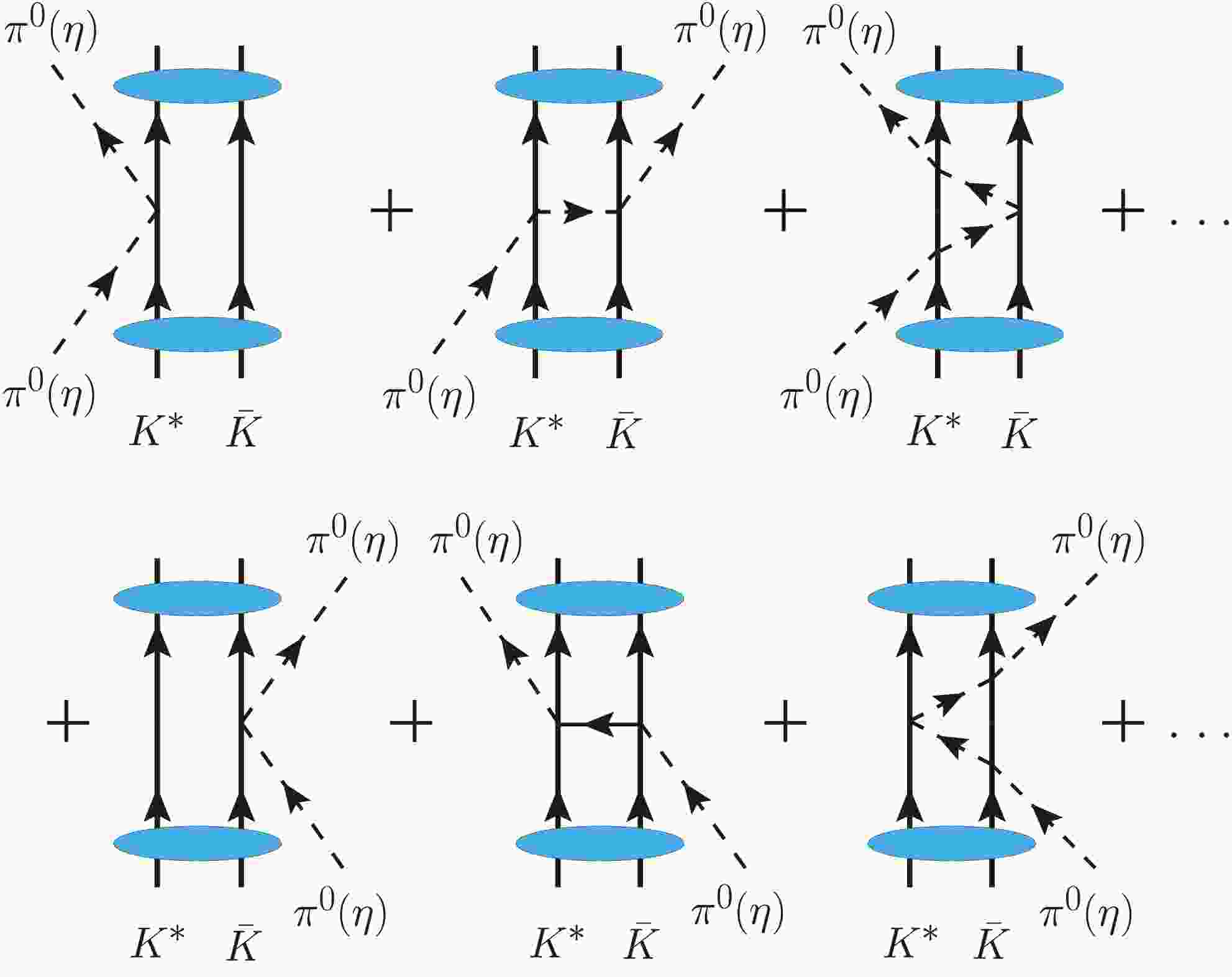
$ \pi^0 $ and η with the$ f_1(1285) $ . Since$ \pi^0 $ and η are identical to their antiparticles, the interaction of$ \pi^0 $ or η with either of the two components of Eq. (1) is the same. This allows us to focus on a single component, namely the interaction of$ \pi^0 $ or η with$ (K^* \bar{K})^{I=0} $ .The FCA includes the diagrams shown in Fig. 1. Owing to the normalization of the scattering matrix for the
$ \pi^0(\eta) $ –$ f_1(1285) $ interaction, rather than for$ \pi^0(\eta) $ scattering with$ K^* $ or$ \bar{K} $ , we write the amplitudes as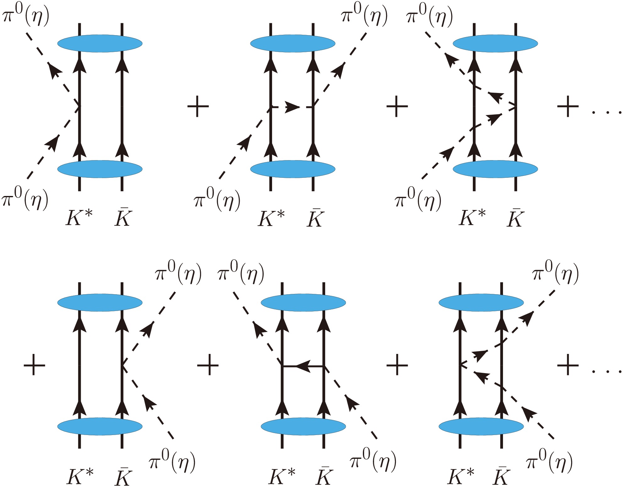
Figure 1. (color online) Diagrams of the conventional FCA describing the interaction of
$ \pi^0 $ or η with the$ K^* \bar{K} $ component of the$ f_1(1285) $ .$ \tilde{t}_1 = \frac{M_c}{m_{K^*}}t_1, \qquad \tilde{t}_2 = \frac{M_c}{m_{\bar{K} }}t_2, $
(2) where
$ M_c $ is the mass of the cluster, i.e., the$ f_1(1285) $ state. The matrices$ t_1 $ and$ t_2 $ describe the scattering of the$ \pi^0 $ and η from the$ K^* $ and$ \bar{K} $ constituents, respectively. It should be noted that$ K^* \bar{K} $ is coupled to$ I=0 $ . In this case (see Ref. [50] for details), one obtains:$ a) $ $ \pi^0 $ scattering$ \begin{split} t_1 = \dfrac{2}{3}\;t_{\pi K^{*}}^{I=3/2}+\dfrac{1}{3}\;t_{\pi K^{*}}^{I=1/2},\quad t_2 = \dfrac{2}{3}\;t_{\pi K}^{I=3/2}+\dfrac{1}{3}\;t_{\pi K}^{I=1/2}, \end{split} $
(3) where we have used the fact that
$ t_{\pi \bar K} $ and$ t_{\pi K} $ are identical;$ b) $ η scattering$ \begin{split} t_1 = t_{\eta K^{*}}^{\,I=1/2},\quad t_2 = t_{\eta \bar K}^{\,I=1/2} = t_{\eta K}^{\,I=1/2}. \end{split} $
(4) The amplitudes
$ t_{\pi K^{*}}^{I=3/2} $ ,$ t_{\pi K^{*}}^{I=1/2} $ ,$ t_{\pi K}^{I=3/2} $ ,$ t_{\pi K}^{I=1/2} $ ,$ t_{\eta K^{*}}^{\,I=1/2} $ , and$ t_{\eta K}^{\,I=1/2} $ that appear in$ t_1,\, t_2 $ of Eqs. (3) and (4) are evaluated in the Appendix.We define the partition matrices
$ \tilde{T}_{ij} $ corresponding to the diagrams in Fig. 1 as the sums of diagrams in which the external particle first interacts with particle i of the cluster and finally interacts with particle j. The matrix$ \tilde{T} $ is then defined as$ \tilde{T}= \left( {\begin{array}{*{20}{c}} {{{\tilde T}_{11}}}&{{{\tilde T}_{12}}}\\ {{{\tilde T}_{21}}}&{{{\tilde T}_{22}}} \end{array}} \right), $
(5) where the elements
$ \tilde{T}_{ij} $ are given by$ \begin{split} & \tilde{T}_{11} = \dfrac{\tilde{t}_1}{1 - \tilde{t}_1 \,\tilde{t}_2 \,G_0^2}, \; \; \; \; \; \; \; \; \; \; \; \; \tilde{T}_{22} = \dfrac{\tilde{t}_2}{1 - \tilde{t}_1\,\tilde{t}_2 \,G_0^2}, \\ & \tilde{T}_{12} = \tilde{T}_{21} = \dfrac{\tilde{t}_1 \,\tilde{t}_2 \, G_0}{1 - \tilde{t}_1 \,\tilde{t}_2 \,G_0^2}, \end{split} $
(6) and
$ G_0(\sqrt{s}) $ denotes the propagator of the external particle, modulated by the wave function of the cluster, and is given by$ \begin{split} G_0(\sqrt{s}) =\;& \int \dfrac{\mathrm{d}^3 q}{(2\pi)^3} \;\dfrac{F_c(q)}{\sqrt{s} - \omega_{ex}(\vec q\,) - \omega_c(\vec q \,) + i \epsilon} \;\dfrac{1}{2 \,\omega_{ex}(\vec q\,)} \\ & \times \dfrac{1}{2 \,\omega_{c}(\vec q\,)} \;\Theta\left(q_{\mathrm{max}}^{(1)} - q_1^*\right) \Theta\left(q_{\mathrm{max}}^{(2)} - q_2^*\right), \end{split} $
(7) with
$ \omega_{ex}(\vec q\,) = \sqrt{m_{ex}^2 + \vec{q}^{\;2}} $ , where$ m_{ex} $ denotes the mass of the external particle ($ \pi^0 $ or η), and$ \omega_c(\vec q\,) = \sqrt{M_c^2 + \vec{q}^{\;2}} $ . The quantity$ F_c(q) $ is the cluster form factor, given by$ \begin{split} F_c(q) =\;& \dfrac{F(q)}{N}, \\ F(q) =\;& \int\nolimits_{\substack{|\vec{p}\,| \lt q_{\mathrm{max}} \\ |\vec{p} - \vec{q}\,| \lt q_{\mathrm{max}}}} \dfrac{\mathrm{d}^3 p}{(2\pi)^3} \; \dfrac{1}{M_c - \omega_{K^*}(\vec{p}\,) - \omega_{\bar K}(\vec{p}\,)} \\ & \times \dfrac{1}{M_c - \omega_{K^*}(\vec{p} - \vec{q}\,) - \omega_{\bar K}(\vec{p} -\vec{q}\,)}, \\ N =\;& F(0) = \int\nolimits_{|\vec{p}\,| \lt q_{\mathrm{max}}} \dfrac{\mathrm{d}^3 p}{(2\pi)^3} \, \left[ \dfrac{1}{M_c - \omega_{K^*}(\vec{p}\,) - \omega_{\bar K}(\vec{p}\,)} \right]^2. \;\; \end{split} $
(8) The magnitude
$ q_{\mathrm{max}} $ in Eq. (8) is the cutoff that regularizes the G loops of the Bethe-Salpeter series in$ t = (1-VG)^{-1}V $ , where V is the potential, in studies of the$ K^* \bar{K} $ interaction that generates the$ f_1(1285) $ molecule [50]. This yields a wave function of the form$ \Psi(p)\sim \frac{\Theta\left(q_{\mathrm{max}}-|\vec{p}\,|\right)} {M_c - \omega_{K^*}(\vec{p}\,) - \omega_{\bar K}(\vec p\,)}. $
(9) The limits of
$ \vec{p} $ in the integral in Eq. (8) ensure its convergence, and$ F(q) $ vanishes for$ |\vec{q}\,| \gt 2\, q_{\mathrm{max}} $ . In Eq. (7), the values of$ q^{(1)}_{\mathrm{max}} $ and$ q^{(2)}_{\mathrm{max}} $ are the cutoffs used to regularize the$ \pi^0(\eta) K^* $ and$ \pi^0(\eta) \bar{K} $ loops when constructing the corresponding scattering matrices,$ t_1 $ and$ t_2 $ . On the other hand,$ q^*_1 $ and$ q^*_2 $ are the$ \pi^0(\eta) $ momenta in the rest frames of$ \pi^0(\eta) K^* $ and$ \pi^0(\eta) \bar{K} $ , respectively. These are obtained by assuming that the transferred momentum is shared between the initial and final particles of the cluster [51, 52]. One has$ \vec{q}^{\,*}_i = \vec{q}\,\left( 1 - \frac{1}{2}\frac{m_{ex}}{m_{ex} + m_{i}} \right), $
(10) where
$ m_1=m_{K^*} $ and$ m_2=m_{\bar K} $ .Elastic unitarity in the
$ \pi^0(\eta) f_1(1285) $ channel is obtained by summing the diagrams shown in Fig. 2. This yields the matrix$ \tilde{T}'_{ij} $ , for which, as before, one sums over all diagrams in which the first scattering occurs with particle i and the final scattering occurs with particle j of the cluster. The$ \tilde{T}' $ matrix is defined as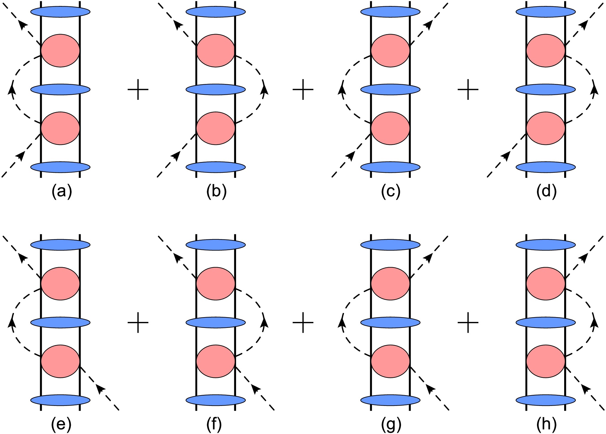
Figure 2. (color online) Diagrams showing the elastic propagation of the external particle and the cluster
$ f_1(1285) $ as a whole.$ \tilde{T}' = \left( {\begin{array}{*{20}{c}} {{{\tilde T'}_{11}}}&{{{\tilde T'}_{12}}}\\ {{{\tilde T'}_{21}}}&{{{\tilde T'}_{22}}} \end{array}} \right), $
(11) and one obtains
$ \tilde{T}' $ by solving a Bethe-Salpeter equation in which$ \tilde{T}_{ij} $ serves as an optical potential:$ \tilde{T}'=\left[ 1-\tilde{T}\,G_c \right]^{-1}\;\tilde{T}, $
(12) where
$ G_c=\left( {\begin{array}{*{20}{c}} {G_c^{(1)}}&0\\ 0&{G_c^{(2)}} \end{array}} \right), $
(13) and
$ \begin{split} G_c^{(i)}(\sqrt{s}) =\;& \int \dfrac{\mathrm{d}^3 q}{(2\pi)^3}\; \dfrac{\left[ F_c^{(i)}(q) \right]^2}{\sqrt{s} - \omega_{ex}(\vec q\,) - \omega_c(\vec q\,) + {\rm i}\epsilon} \\ & \times \dfrac{1}{2\,\omega_{ex}(\vec q\,)} \;\dfrac{1}{2 \, \omega_{c}(\vec q\,)} \;\Theta\left(q_{\mathrm{max}}^{(i)} - q_i^*\right), \end{split} $
(14) with [53]
$ \begin{split} F_c^{(1)}(\vec{q}\,) = F_c\left( \frac{m_{\bar K}}{m_{K^*}+m_{\bar K}} \vec{q}\,\right), \\ F_c^{(2)}(\vec{q}\,) = F_c\left( \frac{m_{K^*}}{m_{K^*}+m_{\bar K}} \vec{q}\,\right). \end{split} $
(15) The amplitudes
$ t_1 $ and$ t_2 $ depend on the invariant masses$ \sqrt{s_1} $ and$ \sqrt{s_2} $ , respectively, which are calculated by assuming that the binding energy of the cluster is absorbed by each particle in the cluster in proportion to its mass, as$ s_1(\pi^0(\eta) K^*) = \left(p_{ex} + p_{K^*}\right)^2 = m_{ex}^2 + \left(\xi \,m_{K^*}\right)^2 + 2\,\xi \,m_{K^*}\,q^0, $
(16) $ s_2(\pi^0(\eta) \bar K) = \left(p_{ex} + p_{\bar K}\right)^2 = m_{ex}^2 + \left(\xi \,m_{\bar K}\right)^2 + 2\,\xi \,m_{\bar K}\,q^0, $
(17) where
$ q^0 $ is the$ \pi^0 $ (η) energy in the cluster rest frame$ q^0=\frac{s-m_{ex}^2-M_c^2}{2 \,M_c}, $
(18) and
$ \xi=\frac{M_c}{m_{K^*} + m_{\bar K}}. $
(19) The final amplitude for
$ \pi^0 (\eta) f_1 $ scattering is given by [37]$ \begin{split} T^{\,\mathrm{tot}} =\sum\limits_{i,j} \tilde{T}'_{ij} =\frac{ \tilde{t}_1+\tilde{t}_2+\left(2 \, G_0-G_c^{(1)}-G_c^{(2)}\right) \tilde{t}_1 \, \tilde{t}_2} {1-G_c^{(1)} \, \tilde{t}_1-G_c^{(2)} \,\tilde{t}_2-\left(G_0^2-G_c^{(1)} \, G_c^{(2)}\right) \tilde{t}_1 \,\tilde{t}_2}, \end{split} $
(20) which enables a straightforward proof of elastic unitarity [37].
-
For the
$ K f_1(1285) $ interaction, we closely follow Ref. [38].In the molecular picture, using the phase conventions for the isospin multiplets
$ (K^+,\,K^0) $ ,$ (\bar{K}^0,\,-K^-) $ ,$ (K^{*+},\,K^{*0}) $ , and$ (\bar{K}^{*0},\,-K^{*-}) $ , the$ f_1(1285) $ is expressed as [28]$ \begin{split} f_1(1285) \equiv\; & -\sqrt{\frac{1}{2}}\left( K^{*+}K^- + K^{*0}\bar{K}^0 - K^{*-}K^+ - \bar{K}^{*0}K^0 \right)\\ =\; &\sqrt{\frac{1}{2}}\left[ \left(K^*\bar{K}\right)^{I=0} + \left(\bar K^* K\right)^{I=0} \right]. \end{split}$
(1) It is necessary to distinguish between the building blocks and the decay channels. The latter contribute to the width of the state because they have available phase space. Although they can be incorporated as components of the wave function, their strength is too small to play a significant role in the formation and mass of the states; therefore, they can be treated perturbatively. This point has been discussed in several works, such as those in Refs. [41, 42]. In particular, from this molecular perspective, the different decay widths of the
$ f_1(1285) $ have been evaluated. The decays into$ a_0(980) \pi $ ,$ f_0(980) \pi $ , and$ K\bar K \pi $ have been successfully tested in Refs. [43, 44]. Further supporting evidence has come from studies of various reactions, including$ K^- p \to f_1(1285) \Lambda $ [45],$ J/\psi \to \phi f_1(1285) $ [46],$ B^0_s \to J/\psi f_1(1285) $ [47],$ \tau \to f_1(1285) \pi \nu_\tau $ [48], and$ \bar B^0 \to J/\psi f_1(1285) $ [49].We study the interaction of
$ \pi^0 $ and η with the$ f_1(1285) $ . Since$ \pi^0 $ and η are identical to their antiparticles, the interaction of$ \pi^0 $ or η with either of the two components of Eq. (1) is the same. This allows us to focus on a single component, namely the interaction of$ \pi^0 $ or η with$ (K^* \bar{K})^{I=0} $ .The FCA includes the diagrams shown in Fig. 1. Owing to the normalization of the scattering matrix for the
$ \pi^0(\eta) $ –$ f_1(1285) $ interaction, rather than for$ \pi^0(\eta) $ scattering with$ K^* $ or$ \bar{K} $ , we write the amplitudes as
Figure 1. (color online) Diagrams of the conventional FCA describing the interaction of
$ \pi^0 $ or η with the$ K^* \bar{K} $ component of the$ f_1(1285) $ .$ \tilde{t}_1 = \frac{M_c}{m_{K^*}}t_1, \qquad \tilde{t}_2 = \frac{M_c}{m_{\bar{K} }}t_2, $
(2) where
$ M_c $ is the mass of the cluster, i.e., the$ f_1(1285) $ state. The matrices$ t_1 $ and$ t_2 $ describe the scattering of the$ \pi^0 $ and η from the$ K^* $ and$ \bar{K} $ constituents, respectively. It should be noted that$ K^* \bar{K} $ is coupled to$ I=0 $ . In this case (see Ref. [50] for details), one obtains:$ a) $ $ \pi^0 $ scattering$ \begin{split} t_1 = \dfrac{2}{3}\;t_{\pi K^{*}}^{I=3/2}+\dfrac{1}{3}\;t_{\pi K^{*}}^{I=1/2},\quad t_2 = \dfrac{2}{3}\;t_{\pi K}^{I=3/2}+\dfrac{1}{3}\;t_{\pi K}^{I=1/2}, \end{split} $
(3) where we have used the fact that
$ t_{\pi \bar K} $ and$ t_{\pi K} $ are identical;$ b) $ η scattering$ \begin{split} t_1 = t_{\eta K^{*}}^{\,I=1/2},\quad t_2 = t_{\eta \bar K}^{\,I=1/2} = t_{\eta K}^{\,I=1/2}. \end{split} $
(4) The amplitudes
$ t_{\pi K^{*}}^{I=3/2} $ ,$ t_{\pi K^{*}}^{I=1/2} $ ,$ t_{\pi K}^{I=3/2} $ ,$ t_{\pi K}^{I=1/2} $ ,$ t_{\eta K^{*}}^{\,I=1/2} $ , and$ t_{\eta K}^{\,I=1/2} $ that appear in$ t_1,\, t_2 $ of Eqs. (3) and (4) are evaluated in the Appendix.We define the partition matrices
$ \tilde{T}_{ij} $ corresponding to the diagrams in Fig. 1 as the sums of diagrams in which the external particle first interacts with particle i of the cluster and finally interacts with particle j. The matrix$ \tilde{T} $ is then defined as$ \tilde{T}= \left( {\begin{array}{*{20}{c}} {{{\tilde T}_{11}}}&{{{\tilde T}_{12}}}\\ {{{\tilde T}_{21}}}&{{{\tilde T}_{22}}} \end{array}} \right), $
(5) where the elements
$ \tilde{T}_{ij} $ are given by$ \begin{split} & \tilde{T}_{11} = \dfrac{\tilde{t}_1}{1 - \tilde{t}_1 \,\tilde{t}_2 \,G_0^2}, \; \; \; \; \; \; \; \; \; \; \; \; \tilde{T}_{22} = \dfrac{\tilde{t}_2}{1 - \tilde{t}_1\,\tilde{t}_2 \,G_0^2}, \\ & \tilde{T}_{12} = \tilde{T}_{21} = \dfrac{\tilde{t}_1 \,\tilde{t}_2 \, G_0}{1 - \tilde{t}_1 \,\tilde{t}_2 \,G_0^2}, \end{split} $
(6) and
$ G_0(\sqrt{s}) $ denotes the propagator of the external particle, modulated by the wave function of the cluster, and is given by$ \begin{split} G_0(\sqrt{s}) =\;& \int \dfrac{\mathrm{d}^3 q}{(2\pi)^3} \;\dfrac{F_c(q)}{\sqrt{s} - \omega_{ex}(\vec q\,) - \omega_c(\vec q \,) + i \epsilon} \;\dfrac{1}{2 \,\omega_{ex}(\vec q\,)} \\ & \times \dfrac{1}{2 \,\omega_{c}(\vec q\,)} \;\Theta\left(q_{\mathrm{max}}^{(1)} - q_1^*\right) \Theta\left(q_{\mathrm{max}}^{(2)} - q_2^*\right), \end{split} $
(7) with
$ \omega_{ex}(\vec q\,) = \sqrt{m_{ex}^2 + \vec{q}^{\;2}} $ , where$ m_{ex} $ denotes the mass of the external particle ($ \pi^0 $ or η), and$ \omega_c(\vec q\,) = \sqrt{M_c^2 + \vec{q}^{\;2}} $ . The quantity$ F_c(q) $ is the cluster form factor, given by$ \begin{split} F_c(q) =\;& \dfrac{F(q)}{N}, \\ F(q) =\;& \int\nolimits_{\substack{|\vec{p}\,| \lt q_{\mathrm{max}} \\ |\vec{p} - \vec{q}\,| \lt q_{\mathrm{max}}}} \dfrac{\mathrm{d}^3 p}{(2\pi)^3} \; \dfrac{1}{M_c - \omega_{K^*}(\vec{p}\,) - \omega_{\bar K}(\vec{p}\,)} \\ & \times \dfrac{1}{M_c - \omega_{K^*}(\vec{p} - \vec{q}\,) - \omega_{\bar K}(\vec{p} -\vec{q}\,)}, \\ N =\;& F(0) = \int\nolimits_{|\vec{p}\,| \lt q_{\mathrm{max}}} \dfrac{\mathrm{d}^3 p}{(2\pi)^3} \, \left[ \dfrac{1}{M_c - \omega_{K^*}(\vec{p}\,) - \omega_{\bar K}(\vec{p}\,)} \right]^2. \;\; \end{split} $
(8) The magnitude
$ q_{\mathrm{max}} $ in Eq. (8) is the cutoff that regularizes the G loops of the Bethe-Salpeter series in$ t = (1-VG)^{-1}V $ , where V is the potential, in studies of the$ K^* \bar{K} $ interaction that generates the$ f_1(1285) $ molecule [50]. This yields a wave function of the form$ \Psi(p)\sim \frac{\Theta\left(q_{\mathrm{max}}-|\vec{p}\,|\right)} {M_c - \omega_{K^*}(\vec{p}\,) - \omega_{\bar K}(\vec p\,)}. $
(9) The limits of
$ \vec{p} $ in the integral in Eq. (8) ensure its convergence, and$ F(q) $ vanishes for$ |\vec{q}\,| \gt 2\, q_{\mathrm{max}} $ . In Eq. (7), the values of$ q^{(1)}_{\mathrm{max}} $ and$ q^{(2)}_{\mathrm{max}} $ are the cutoffs used to regularize the$ \pi^0(\eta) K^* $ and$ \pi^0(\eta) \bar{K} $ loops when constructing the corresponding scattering matrices,$ t_1 $ and$ t_2 $ . On the other hand,$ q^*_1 $ and$ q^*_2 $ are the$ \pi^0(\eta) $ momenta in the rest frames of$ \pi^0(\eta) K^* $ and$ \pi^0(\eta) \bar{K} $ , respectively. These are obtained by assuming that the transferred momentum is shared between the initial and final particles of the cluster [51, 52]. One has$ \vec{q}^{\,*}_i = \vec{q}\,\left( 1 - \frac{1}{2}\frac{m_{ex}}{m_{ex} + m_{i}} \right), $
(10) where
$ m_1=m_{K^*} $ and$ m_2=m_{\bar K} $ .Elastic unitarity in the
$ \pi^0(\eta) f_1(1285) $ channel is obtained by summing the diagrams shown in Fig. 2. This yields the matrix$ \tilde{T}'_{ij} $ , for which, as before, one sums over all diagrams in which the first scattering occurs with particle i and the final scattering occurs with particle j of the cluster. The$ \tilde{T}' $ matrix is defined as
Figure 2. (color online) Diagrams showing the elastic propagation of the external particle and the cluster
$ f_1(1285) $ as a whole.$ \tilde{T}' = \left( {\begin{array}{*{20}{c}} {{{\tilde T'}_{11}}}&{{{\tilde T'}_{12}}}\\ {{{\tilde T'}_{21}}}&{{{\tilde T'}_{22}}} \end{array}} \right), $
(11) and one obtains
$ \tilde{T}' $ by solving a Bethe-Salpeter equation in which$ \tilde{T}_{ij} $ serves as an optical potential:$ \tilde{T}'=\left[ 1-\tilde{T}\,G_c \right]^{-1}\;\tilde{T}, $
(12) where
$ G_c=\left( {\begin{array}{*{20}{c}} {G_c^{(1)}}&0\\ 0&{G_c^{(2)}} \end{array}} \right), $
(13) and
$ \begin{split} G_c^{(i)}(\sqrt{s}) =\;& \int \dfrac{\mathrm{d}^3 q}{(2\pi)^3}\; \dfrac{\left[ F_c^{(i)}(q) \right]^2}{\sqrt{s} - \omega_{ex}(\vec q\,) - \omega_c(\vec q\,) + {\rm i}\epsilon} \\ & \times \dfrac{1}{2\,\omega_{ex}(\vec q\,)} \;\dfrac{1}{2 \, \omega_{c}(\vec q\,)} \;\Theta\left(q_{\mathrm{max}}^{(i)} - q_i^*\right), \end{split} $
(14) with [53]
$ \begin{split} F_c^{(1)}(\vec{q}\,) = F_c\left( \frac{m_{\bar K}}{m_{K^*}+m_{\bar K}} \vec{q}\,\right), \\ F_c^{(2)}(\vec{q}\,) = F_c\left( \frac{m_{K^*}}{m_{K^*}+m_{\bar K}} \vec{q}\,\right). \end{split} $
(15) The amplitudes
$ t_1 $ and$ t_2 $ depend on the invariant masses$ \sqrt{s_1} $ and$ \sqrt{s_2} $ , respectively, which are calculated by assuming that the binding energy of the cluster is absorbed by each particle in the cluster in proportion to its mass, as$ s_1(\pi^0(\eta) K^*) = \left(p_{ex} + p_{K^*}\right)^2 = m_{ex}^2 + \left(\xi \,m_{K^*}\right)^2 + 2\,\xi \,m_{K^*}\,q^0, $
(16) $ s_2(\pi^0(\eta) \bar K) = \left(p_{ex} + p_{\bar K}\right)^2 = m_{ex}^2 + \left(\xi \,m_{\bar K}\right)^2 + 2\,\xi \,m_{\bar K}\,q^0, $
(17) where
$ q^0 $ is the$ \pi^0 $ (η) energy in the cluster rest frame$ q^0=\frac{s-m_{ex}^2-M_c^2}{2 \,M_c}, $
(18) and
$ \xi=\frac{M_c}{m_{K^*} + m_{\bar K}}. $
(19) The final amplitude for
$ \pi^0 (\eta) f_1 $ scattering is given by [37]$ \begin{split} T^{\,\mathrm{tot}} =\sum\limits_{i,j} \tilde{T}'_{ij} =\frac{ \tilde{t}_1+\tilde{t}_2+\left(2 \, G_0-G_c^{(1)}-G_c^{(2)}\right) \tilde{t}_1 \, \tilde{t}_2} {1-G_c^{(1)} \, \tilde{t}_1-G_c^{(2)} \,\tilde{t}_2-\left(G_0^2-G_c^{(1)} \, G_c^{(2)}\right) \tilde{t}_1 \,\tilde{t}_2}, \end{split} $
(20) which enables a straightforward proof of elastic unitarity [37].
-
For the
$ K f_1(1285) $ interaction, we closely follow Ref. [38].In the molecular picture, using the phase conventions for the isospin multiplets
$ (K^+,\,K^0) $ ,$ (\bar{K}^0,\,-K^-) $ ,$ (K^{*+},\,K^{*0}) $ , and$ (\bar{K}^{*0},\,-K^{*-}) $ , the$ f_1(1285) $ is expressed as [28]$ \begin{split} f_1(1285) \equiv\; & -\sqrt{\frac{1}{2}}\left( K^{*+}K^- + K^{*0}\bar{K}^0 - K^{*-}K^+ - \bar{K}^{*0}K^0 \right)\\ =\; &\sqrt{\frac{1}{2}}\left[ \left(K^*\bar{K}\right)^{I=0} + \left(\bar K^* K\right)^{I=0} \right]. \end{split}$
(1) It is necessary to distinguish between the building blocks and the decay channels. The latter contribute to the width of the state because they have available phase space. Although they can be incorporated as components of the wave function, their strength is too small to play a significant role in the formation and mass of the states; therefore, they can be treated perturbatively. This point has been discussed in several works, such as those in Refs. [41, 42]. In particular, from this molecular perspective, the different decay widths of the
$ f_1(1285) $ have been evaluated. The decays into$ a_0(980) \pi $ ,$ f_0(980) \pi $ , and$ K\bar K \pi $ have been successfully tested in Refs. [43, 44]. Further supporting evidence has come from studies of various reactions, including$ K^- p \to f_1(1285) \Lambda $ [45],$ J/\psi \to \phi f_1(1285) $ [46],$ B^0_s \to J/\psi f_1(1285) $ [47],$ \tau \to f_1(1285) \pi \nu_\tau $ [48], and$ \bar B^0 \to J/\psi f_1(1285) $ [49].We study the interaction of
$ \pi^0 $ and η with the$ f_1(1285) $ . Since$ \pi^0 $ and η are identical to their antiparticles, the interaction of$ \pi^0 $ or η with either of the two components of Eq. (1) is the same. This allows us to focus on a single component, namely the interaction of$ \pi^0 $ or η with$ (K^* \bar{K})^{I=0} $ .The FCA includes the diagrams shown in Fig. 1. Owing to the normalization of the scattering matrix for the
$ \pi^0(\eta) $ –$ f_1(1285) $ interaction, rather than for$ \pi^0(\eta) $ scattering with$ K^* $ or$ \bar{K} $ , we write the amplitudes as
Figure 1. (color online) Diagrams of the conventional FCA describing the interaction of
$ \pi^0 $ or η with the$ K^* \bar{K} $ component of the$ f_1(1285) $ .$ \tilde{t}_1 = \frac{M_c}{m_{K^*}}t_1, \qquad \tilde{t}_2 = \frac{M_c}{m_{\bar{K} }}t_2, $
(2) where
$ M_c $ is the mass of the cluster, i.e., the$ f_1(1285) $ state. The matrices$ t_1 $ and$ t_2 $ describe the scattering of the$ \pi^0 $ and η from the$ K^* $ and$ \bar{K} $ constituents, respectively. It should be noted that$ K^* \bar{K} $ is coupled to$ I=0 $ . In this case (see Ref. [50] for details), one obtains:$ a) $ $ \pi^0 $ scattering$ \begin{split} t_1 = \dfrac{2}{3}\;t_{\pi K^{*}}^{I=3/2}+\dfrac{1}{3}\;t_{\pi K^{*}}^{I=1/2},\quad t_2 = \dfrac{2}{3}\;t_{\pi K}^{I=3/2}+\dfrac{1}{3}\;t_{\pi K}^{I=1/2}, \end{split} $
(3) where we have used the fact that
$ t_{\pi \bar K} $ and$ t_{\pi K} $ are identical;$ b) $ η scattering$ \begin{split} t_1 = t_{\eta K^{*}}^{\,I=1/2},\quad t_2 = t_{\eta \bar K}^{\,I=1/2} = t_{\eta K}^{\,I=1/2}. \end{split} $
(4) The amplitudes
$ t_{\pi K^{*}}^{I=3/2} $ ,$ t_{\pi K^{*}}^{I=1/2} $ ,$ t_{\pi K}^{I=3/2} $ ,$ t_{\pi K}^{I=1/2} $ ,$ t_{\eta K^{*}}^{\,I=1/2} $ , and$ t_{\eta K}^{\,I=1/2} $ that appear in$ t_1,\, t_2 $ of Eqs. (3) and (4) are evaluated in the Appendix.We define the partition matrices
$ \tilde{T}_{ij} $ corresponding to the diagrams in Fig. 1 as the sums of diagrams in which the external particle first interacts with particle i of the cluster and finally interacts with particle j. The matrix$ \tilde{T} $ is then defined as$ \tilde{T}= \left( {\begin{array}{*{20}{c}} {{{\tilde T}_{11}}}&{{{\tilde T}_{12}}}\\ {{{\tilde T}_{21}}}&{{{\tilde T}_{22}}} \end{array}} \right), $
(5) where the elements
$ \tilde{T}_{ij} $ are given by$ \begin{split} & \tilde{T}_{11} = \dfrac{\tilde{t}_1}{1 - \tilde{t}_1 \,\tilde{t}_2 \,G_0^2}, \; \; \; \; \; \; \; \; \; \; \; \; \tilde{T}_{22} = \dfrac{\tilde{t}_2}{1 - \tilde{t}_1\,\tilde{t}_2 \,G_0^2}, \\ & \tilde{T}_{12} = \tilde{T}_{21} = \dfrac{\tilde{t}_1 \,\tilde{t}_2 \, G_0}{1 - \tilde{t}_1 \,\tilde{t}_2 \,G_0^2}, \end{split} $
(6) and
$ G_0(\sqrt{s}) $ denotes the propagator of the external particle, modulated by the wave function of the cluster, and is given by$ \begin{split} G_0(\sqrt{s}) =\;& \int \dfrac{\mathrm{d}^3 q}{(2\pi)^3} \;\dfrac{F_c(q)}{\sqrt{s} - \omega_{ex}(\vec q\,) - \omega_c(\vec q \,) + i \epsilon} \;\dfrac{1}{2 \,\omega_{ex}(\vec q\,)} \\ & \times \dfrac{1}{2 \,\omega_{c}(\vec q\,)} \;\Theta\left(q_{\mathrm{max}}^{(1)} - q_1^*\right) \Theta\left(q_{\mathrm{max}}^{(2)} - q_2^*\right), \end{split} $
(7) with
$ \omega_{ex}(\vec q\,) = \sqrt{m_{ex}^2 + \vec{q}^{\;2}} $ , where$ m_{ex} $ denotes the mass of the external particle ($ \pi^0 $ or η), and$ \omega_c(\vec q\,) = \sqrt{M_c^2 + \vec{q}^{\;2}} $ . The quantity$ F_c(q) $ is the cluster form factor, given by$ \begin{split} F_c(q) =\;& \dfrac{F(q)}{N}, \\ F(q) =\;& \int\nolimits_{\substack{|\vec{p}\,| \lt q_{\mathrm{max}} \\ |\vec{p} - \vec{q}\,| \lt q_{\mathrm{max}}}} \dfrac{\mathrm{d}^3 p}{(2\pi)^3} \; \dfrac{1}{M_c - \omega_{K^*}(\vec{p}\,) - \omega_{\bar K}(\vec{p}\,)} \\ & \times \dfrac{1}{M_c - \omega_{K^*}(\vec{p} - \vec{q}\,) - \omega_{\bar K}(\vec{p} -\vec{q}\,)}, \\ N =\;& F(0) = \int\nolimits_{|\vec{p}\,| \lt q_{\mathrm{max}}} \dfrac{\mathrm{d}^3 p}{(2\pi)^3} \, \left[ \dfrac{1}{M_c - \omega_{K^*}(\vec{p}\,) - \omega_{\bar K}(\vec{p}\,)} \right]^2. \;\; \end{split} $
(8) The magnitude
$ q_{\mathrm{max}} $ in Eq. (8) is the cutoff that regularizes the G loops of the Bethe-Salpeter series in$ t = (1-VG)^{-1}V $ , where V is the potential, in studies of the$ K^* \bar{K} $ interaction that generates the$ f_1(1285) $ molecule [50]. This yields a wave function of the form$ \Psi(p)\sim \frac{\Theta\left(q_{\mathrm{max}}-|\vec{p}\,|\right)} {M_c - \omega_{K^*}(\vec{p}\,) - \omega_{\bar K}(\vec p\,)}. $
(9) The limits of
$ \vec{p} $ in the integral in Eq. (8) ensure its convergence, and$ F(q) $ vanishes for$ |\vec{q}\,| \gt 2\, q_{\mathrm{max}} $ . In Eq. (7), the values of$ q^{(1)}_{\mathrm{max}} $ and$ q^{(2)}_{\mathrm{max}} $ are the cutoffs used to regularize the$ \pi^0(\eta) K^* $ and$ \pi^0(\eta) \bar{K} $ loops when constructing the corresponding scattering matrices,$ t_1 $ and$ t_2 $ . On the other hand,$ q^*_1 $ and$ q^*_2 $ are the$ \pi^0(\eta) $ momenta in the rest frames of$ \pi^0(\eta) K^* $ and$ \pi^0(\eta) \bar{K} $ , respectively. These are obtained by assuming that the transferred momentum is shared between the initial and final particles of the cluster [51, 52]. One has$ \vec{q}^{\,*}_i = \vec{q}\,\left( 1 - \frac{1}{2}\frac{m_{ex}}{m_{ex} + m_{i}} \right), $
(10) where
$ m_1=m_{K^*} $ and$ m_2=m_{\bar K} $ .Elastic unitarity in the
$ \pi^0(\eta) f_1(1285) $ channel is obtained by summing the diagrams shown in Fig. 2. This yields the matrix$ \tilde{T}'_{ij} $ , for which, as before, one sums over all diagrams in which the first scattering occurs with particle i and the final scattering occurs with particle j of the cluster. The$ \tilde{T}' $ matrix is defined as
Figure 2. (color online) Diagrams showing the elastic propagation of the external particle and the cluster
$ f_1(1285) $ as a whole.$ \tilde{T}' = \left( {\begin{array}{*{20}{c}} {{{\tilde T'}_{11}}}&{{{\tilde T'}_{12}}}\\ {{{\tilde T'}_{21}}}&{{{\tilde T'}_{22}}} \end{array}} \right), $
(11) and one obtains
$ \tilde{T}' $ by solving a Bethe-Salpeter equation in which$ \tilde{T}_{ij} $ serves as an optical potential:$ \tilde{T}'=\left[ 1-\tilde{T}\,G_c \right]^{-1}\;\tilde{T}, $
(12) where
$ G_c=\left( {\begin{array}{*{20}{c}} {G_c^{(1)}}&0\\ 0&{G_c^{(2)}} \end{array}} \right), $
(13) and
$ \begin{split} G_c^{(i)}(\sqrt{s}) =\;& \int \dfrac{\mathrm{d}^3 q}{(2\pi)^3}\; \dfrac{\left[ F_c^{(i)}(q) \right]^2}{\sqrt{s} - \omega_{ex}(\vec q\,) - \omega_c(\vec q\,) + {\rm i}\epsilon} \\ & \times \dfrac{1}{2\,\omega_{ex}(\vec q\,)} \;\dfrac{1}{2 \, \omega_{c}(\vec q\,)} \;\Theta\left(q_{\mathrm{max}}^{(i)} - q_i^*\right), \end{split} $
(14) with [53]
$ \begin{split} F_c^{(1)}(\vec{q}\,) = F_c\left( \frac{m_{\bar K}}{m_{K^*}+m_{\bar K}} \vec{q}\,\right), \\ F_c^{(2)}(\vec{q}\,) = F_c\left( \frac{m_{K^*}}{m_{K^*}+m_{\bar K}} \vec{q}\,\right). \end{split} $
(15) The amplitudes
$ t_1 $ and$ t_2 $ depend on the invariant masses$ \sqrt{s_1} $ and$ \sqrt{s_2} $ , respectively, which are calculated by assuming that the binding energy of the cluster is absorbed by each particle in the cluster in proportion to its mass, as$ s_1(\pi^0(\eta) K^*) = \left(p_{ex} + p_{K^*}\right)^2 = m_{ex}^2 + \left(\xi \,m_{K^*}\right)^2 + 2\,\xi \,m_{K^*}\,q^0, $
(16) $ s_2(\pi^0(\eta) \bar K) = \left(p_{ex} + p_{\bar K}\right)^2 = m_{ex}^2 + \left(\xi \,m_{\bar K}\right)^2 + 2\,\xi \,m_{\bar K}\,q^0, $
(17) where
$ q^0 $ is the$ \pi^0 $ (η) energy in the cluster rest frame$ q^0=\frac{s-m_{ex}^2-M_c^2}{2 \,M_c}, $
(18) and
$ \xi=\frac{M_c}{m_{K^*} + m_{\bar K}}. $
(19) The final amplitude for
$ \pi^0 (\eta) f_1 $ scattering is given by [37]$ \begin{split} T^{\,\mathrm{tot}} =\sum\limits_{i,j} \tilde{T}'_{ij} =\frac{ \tilde{t}_1+\tilde{t}_2+\left(2 \, G_0-G_c^{(1)}-G_c^{(2)}\right) \tilde{t}_1 \, \tilde{t}_2} {1-G_c^{(1)} \, \tilde{t}_1-G_c^{(2)} \,\tilde{t}_2-\left(G_0^2-G_c^{(1)} \, G_c^{(2)}\right) \tilde{t}_1 \,\tilde{t}_2}, \end{split} $
(20) which enables a straightforward proof of elastic unitarity [37].
-
Using the relationship between our amplitude and the standard quantum-mechanical amplitude,
$ f^{\mathrm{QM}} $ , we have$ \begin{split} -8\pi\sqrt{s} \left(T^{\,\mathrm{tot}}\right)^{-1} = (f^{\mathrm{QM}})^{-1} \simeq -\dfrac{1}{a} + \dfrac{1}{2}\,r_0 \,q_{\mathrm{cm}}^2 - {\rm i} q_{\mathrm{cm}}, \end{split} $
(21) where
$ q_{\mathrm{cm}} $ is the$ \pi^0(\eta) $ momentum in the$ \pi^0(\eta) f_1 $ rest frame. Examining the amplitude near the threshold, it follows immediately that$ a = \dfrac{T^{\,\mathrm{tot}}}{8\,\pi\sqrt{s}}\,\Big|_{\mathrm{th}}, $
(22) $ r_0 = \dfrac{1}{\mu} \left[ \dfrac{\partial}{\partial \sqrt{s}} \left( -8\,\pi\sqrt{s} \,\left(T^{\,\mathrm{tot}}\right)^{-1} + {\rm i}q_{\mathrm{cm}} \right) \right]_{\mathrm{th}}, $
(23) where μ denotes the reduced mass of the
$ \pi^0(\eta) f_1 $ system. -
Using the relationship between our amplitude and the standard quantum-mechanical amplitude,
$ f^{\mathrm{QM}} $ , we have$ \begin{split} -8\pi\sqrt{s} \left(T^{\,\mathrm{tot}}\right)^{-1} = (f^{\mathrm{QM}})^{-1} \simeq -\dfrac{1}{a} + \dfrac{1}{2}\,r_0 \,q_{\mathrm{cm}}^2 - {\rm i} q_{\mathrm{cm}}, \end{split} $
(21) where
$ q_{\mathrm{cm}} $ is the$ \pi^0(\eta) $ momentum in the$ \pi^0(\eta) f_1 $ rest frame. Examining the amplitude near the threshold, it follows immediately that$ a = \dfrac{T^{\,\mathrm{tot}}}{8\,\pi\sqrt{s}}\,\Big|_{\mathrm{th}}, $
(22) $ r_0 = \dfrac{1}{\mu} \left[ \dfrac{\partial}{\partial \sqrt{s}} \left( -8\,\pi\sqrt{s} \,\left(T^{\,\mathrm{tot}}\right)^{-1} + {\rm i}q_{\mathrm{cm}} \right) \right]_{\mathrm{th}}, $
(23) where μ denotes the reduced mass of the
$ \pi^0(\eta) f_1 $ system. -
Using the relationship between our amplitude and the standard quantum-mechanical amplitude,
$ f^{\mathrm{QM}} $ , we have$ \begin{split} -8\pi\sqrt{s} \left(T^{\,\mathrm{tot}}\right)^{-1} = (f^{\mathrm{QM}})^{-1} \simeq -\dfrac{1}{a} + \dfrac{1}{2}\,r_0 \,q_{\mathrm{cm}}^2 - {\rm i} q_{\mathrm{cm}}, \end{split} $
(21) where
$ q_{\mathrm{cm}} $ is the$ \pi^0(\eta) $ momentum in the$ \pi^0(\eta) f_1 $ rest frame. Examining the amplitude near the threshold, it follows immediately that$ a = \dfrac{T^{\,\mathrm{tot}}}{8\,\pi\sqrt{s}}\,\Big|_{\mathrm{th}}, $
(22) $ r_0 = \dfrac{1}{\mu} \left[ \dfrac{\partial}{\partial \sqrt{s}} \left( -8\,\pi\sqrt{s} \,\left(T^{\,\mathrm{tot}}\right)^{-1} + {\rm i}q_{\mathrm{cm}} \right) \right]_{\mathrm{th}}, $
(23) where μ denotes the reduced mass of the
$ \pi^0(\eta) f_1 $ system. -
The
$ \pi^0(\eta) f_1 $ correlation function is then given by$ \begin{split} C_{\pi^0(\eta)f_1}(p) =\;& 1 + 4\pi \int_{0}^{\infty} \mathrm{d}r \, r^2 \,S_{12}(r) \\ & \times \left\{ \left|j_0(pr) + TG\right|^2 - j_0^2(pr) \right\}, \end{split} $
(24) where
$ TG=\left( \tilde{T}'_{11}+\tilde{T}'_{21} \right)G_1(\sqrt{s},r)+\left( \tilde{T}'_{12}+\tilde{T}'_{22} \right)G_2(\sqrt{s},r), $
(25) with
$ S_{12}(r)=\frac{1}{\left( 4\pi R^2 \right)^{3/2}}\;{\rm e}^{-r^2/4R^2}, $
(26) where R is the radius of the source and
$ G_1,\,G_2 $ are given by$ \begin{split} G_i(\sqrt{s},r) =\;& \int \dfrac{\mathrm{d}^3 q}{(2\pi)^3} \; \dfrac{ j_0(qr)\,F_c^{(i)}(q) }{\sqrt{s} - \omega_{ex}(\vec q\,) - \omega_c(\vec q\,) + {\rm i}\epsilon} \\ & \times \dfrac{1}{2\,\omega_{ex}(\vec q\,)} \;\dfrac{1}{2\,\omega_{c}(\vec q\,)}\;\Theta\left(q_{\mathrm{max}}^{(i)} - q_i^*\right). \end{split} $
(27) -
The
$ \pi^0(\eta) f_1 $ correlation function is then given by$ \begin{split} C_{\pi^0(\eta)f_1}(p) =\;& 1 + 4\pi \int_{0}^{\infty} \mathrm{d}r \, r^2 \,S_{12}(r) \\ & \times \left\{ \left|j_0(pr) + TG\right|^2 - j_0^2(pr) \right\}, \end{split} $
(24) where
$ TG=\left( \tilde{T}'_{11}+\tilde{T}'_{21} \right)G_1(\sqrt{s},r)+\left( \tilde{T}'_{12}+\tilde{T}'_{22} \right)G_2(\sqrt{s},r), $
(25) with
$ S_{12}(r)=\frac{1}{\left( 4\pi R^2 \right)^{3/2}}\;{\rm e}^{-r^2/4R^2}, $
(26) where R is the radius of the source and
$ G_1,\,G_2 $ are given by$ \begin{split} G_i(\sqrt{s},r) =\;& \int \dfrac{\mathrm{d}^3 q}{(2\pi)^3} \; \dfrac{ j_0(qr)\,F_c^{(i)}(q) }{\sqrt{s} - \omega_{ex}(\vec q\,) - \omega_c(\vec q\,) + {\rm i}\epsilon} \\ & \times \dfrac{1}{2\,\omega_{ex}(\vec q\,)} \;\dfrac{1}{2\,\omega_{c}(\vec q\,)}\;\Theta\left(q_{\mathrm{max}}^{(i)} - q_i^*\right). \end{split} $
(27) -
The
$ \pi^0(\eta) f_1 $ correlation function is then given by$ \begin{split} C_{\pi^0(\eta)f_1}(p) =\;& 1 + 4\pi \int_{0}^{\infty} \mathrm{d}r \, r^2 \,S_{12}(r) \\ & \times \left\{ \left|j_0(pr) + TG\right|^2 - j_0^2(pr) \right\}, \end{split} $
(24) where
$ TG=\left( \tilde{T}'_{11}+\tilde{T}'_{21} \right)G_1(\sqrt{s},r)+\left( \tilde{T}'_{12}+\tilde{T}'_{22} \right)G_2(\sqrt{s},r), $
(25) with
$ S_{12}(r)=\frac{1}{\left( 4\pi R^2 \right)^{3/2}}\;{\rm e}^{-r^2/4R^2}, $
(26) where R is the radius of the source and
$ G_1,\,G_2 $ are given by$ \begin{split} G_i(\sqrt{s},r) =\;& \int \dfrac{\mathrm{d}^3 q}{(2\pi)^3} \; \dfrac{ j_0(qr)\,F_c^{(i)}(q) }{\sqrt{s} - \omega_{ex}(\vec q\,) - \omega_c(\vec q\,) + {\rm i}\epsilon} \\ & \times \dfrac{1}{2\,\omega_{ex}(\vec q\,)} \;\dfrac{1}{2\,\omega_{c}(\vec q\,)}\;\Theta\left(q_{\mathrm{max}}^{(i)} - q_i^*\right). \end{split} $
(27) -
The first results we present are for the scattering length a and the effective range
$ r_0 $ . We obtain:$ a) $ for the$ \pi^0 f_1 $ system$ a = -0.05\,\mathrm{fm}, $
(28) $ r_0 = (-47.37-{\rm i}\, 0.49)\,\mathrm{fm}. $
(29) This is a special case characterized by a very small scattering length and a large effective range.
$ b) $ for the$ \eta f_1 $ system$ a = (0.29-{\rm i}\, 0.08)\,\mathrm{fm}, $
(30) $ r_0 = (0.47+{\rm i}\, 0.50)\,\mathrm{fm}. $
(31) In the latter case, the value of a is approximately half that for the
$ K f_1 $ system, and$ r_0 $ is also approximately half as large as that for the$ K f_1 $ system but has the opposite sign.Next, we show the results for the total
$ \pi^0 f_1(1285) $ amplitude as a function of$ \sqrt{s} $ in Fig. 3. In Fig. 4, we show the results for$ \eta f_1(1285) $ scattering.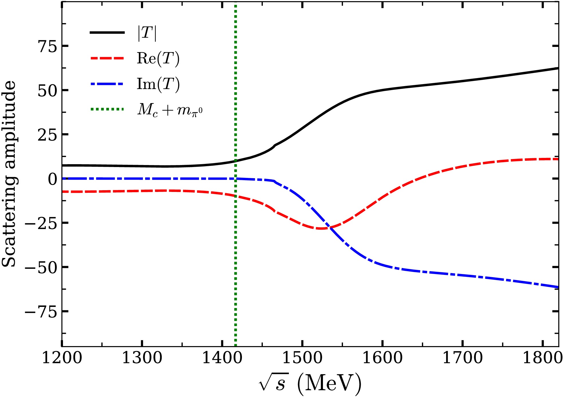
Figure 3. (color online) The
$ \pi^0 f_1(1285) $ scattering amplitude$ T_{\pi^0 f_1}^{\,\mathrm{tot}} $ as a function of$ \sqrt{s} $ .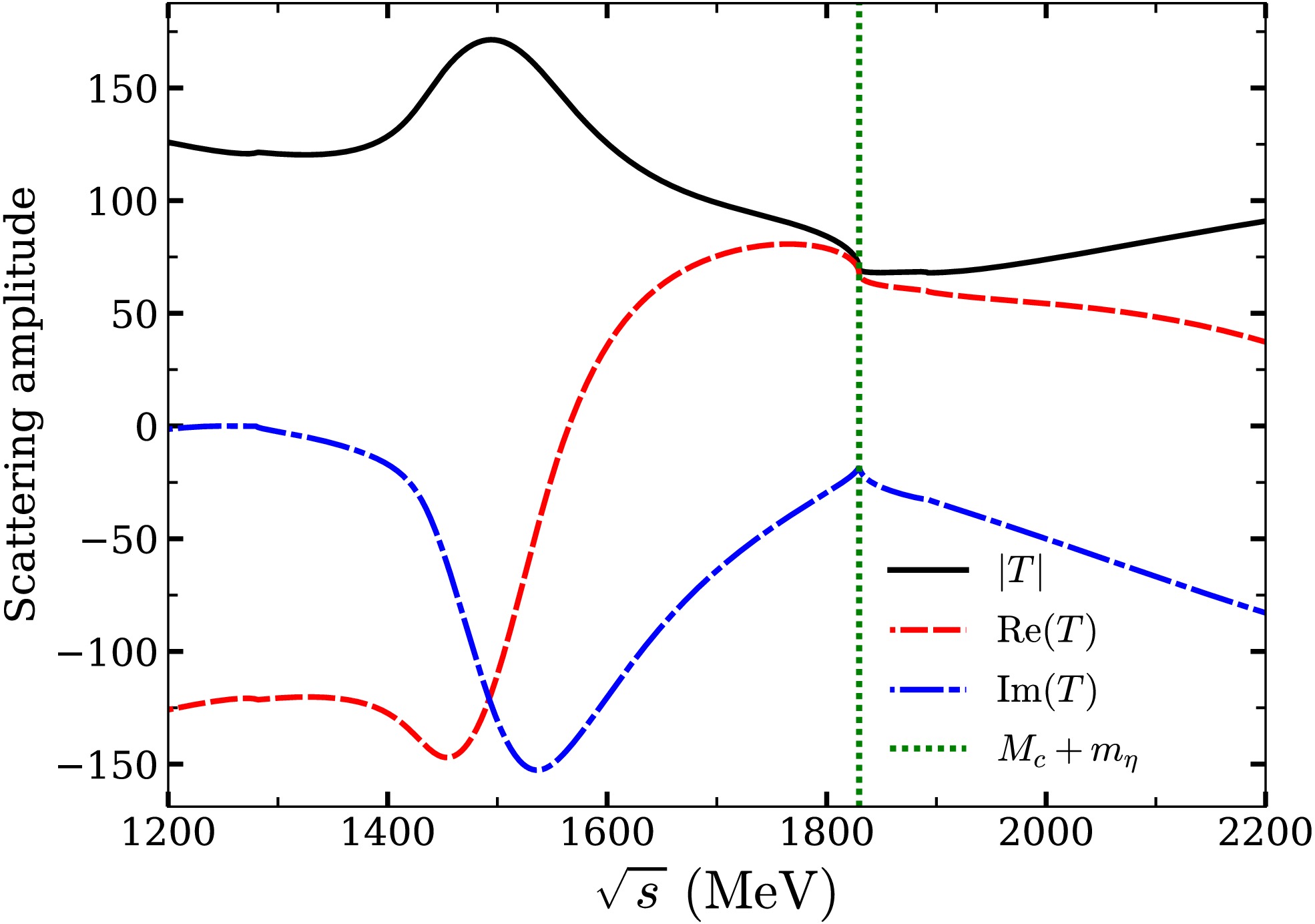
Figure 4. (color online) The
$ \eta f_1(1285) $ scattering amplitude$ T_{\eta f_1}^{\,\mathrm{tot}} $ as a function of$ \sqrt{s} $ .In Fig. 3, the
$ \pi^0 f_1(1285) $ amplitude exhibits smooth behavior at and below threshold. However, in the region$ 1500-1600 \ {\rm{ MeV}} $ , a notable structure appears. The amplitude exhibits resonance-like behavior with a phase of$ \pi/2 $ , which corresponds to having the roles of the real and imaginary parts interchanged. The modulus of the real part displays a peak, whereas the imaginary part resembles the real part of a Breit-Wigner resonance with an added constant. It is unclear whether this structure is related to the$ \pi_1(1400-1600) $ state reported in the PDG, but it is noteworthy that a structure in the amplitude emerges precisely at the energy where the$ \pi_1(1400-1600) $ has been claimed experimentally.Concerning the
$ \eta f_1 $ amplitude, we first note that we do not observe any structure around$ 1855 \ {\rm{ MeV}} $ that could be associated with the$ \eta_1(1855) $ . We can only state that we obtain a pronounced cusp structure around the threshold at$ 1830 \ {\rm{ MeV}} $ . Second, we observe some structure around$ 1500 \ {\rm{ MeV}} $ . However, this is about$ 330 \ {\rm{ MeV}} $ below the$ \eta f_1(1285) $ threshold, where we are reluctant to trust our results. We can reasonably trust our results within approximately$ 150 \ {\rm{ MeV}} $ above and below threshold, corresponding to the energy range of the correlation functions in Ref. [34]. Thus, we prefer not to make any claim concerning this structure.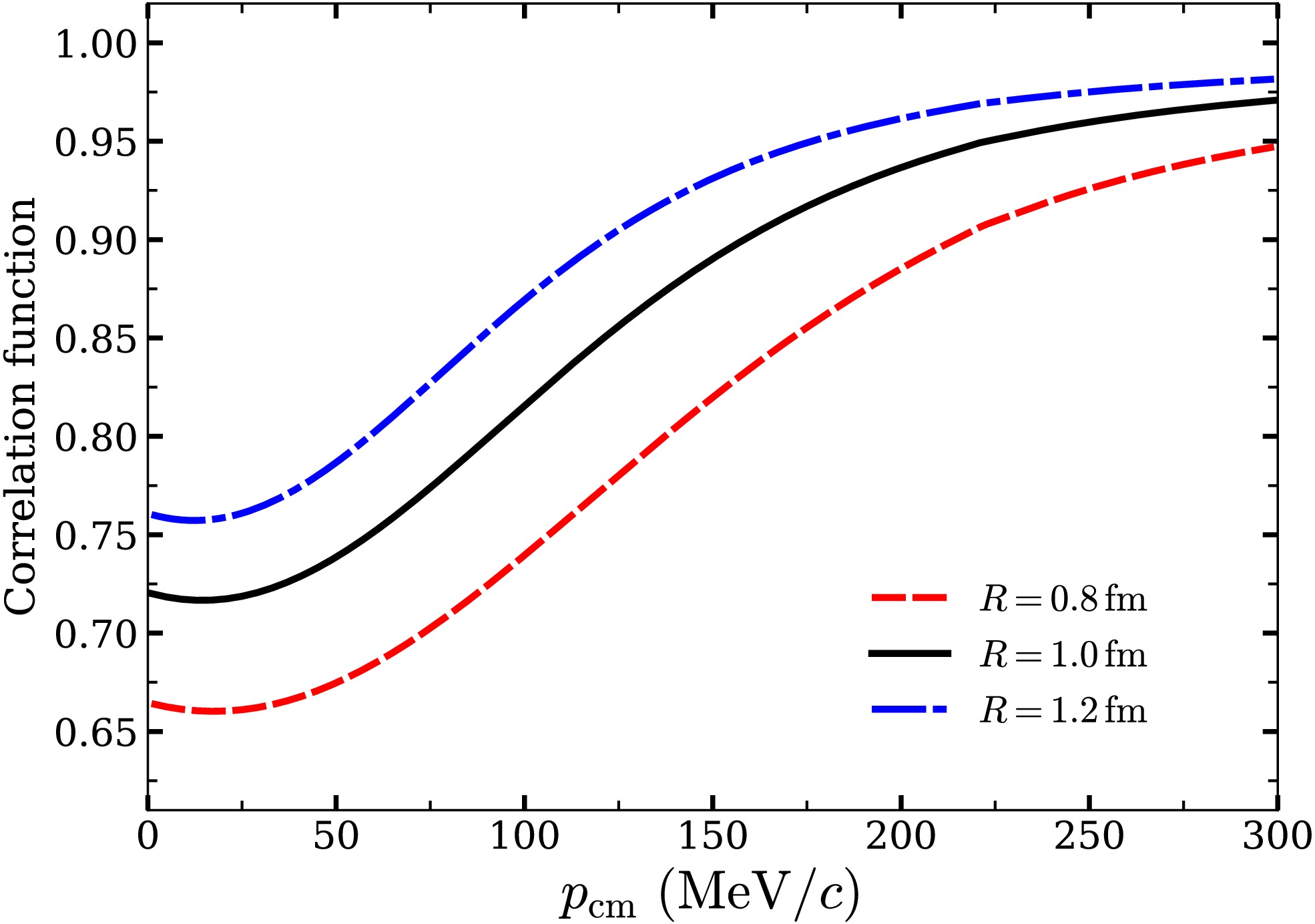
Figure 6. (color online) Correlation functions for the
$ \eta f_1(1285) $ system as functions of the momentum$ p_{\rm{cm}} $ for different values of the source radius R.Next, we present the results for the correlation functions. Figure 5 shows the results for the
$ \pi^0 f_1(1285) $ correlation function. Figure 6 shows the corresponding results for the$ \eta f_1(1285) $ correlation function. For the$ \pi^0 f_1 $ case, the correlation function has values very close to$ 1 $ , indicating a weak interaction. The value of the correlation function decreases with increasing momentum at small values of$ p_{\rm{cm}} $ . The kink appearing around$ p_{\rm{cm}} \simeq 110 \ {\rm{ MeV}} $ corresponds to the opening of the$ \pi K $ threshold in the$ t_2 $ amplitude, as can be seen by applying Eq. (17), which relates s to$ s_2 $ . This corresponds to$ \sqrt{s} \simeq 1465 \ {\rm{ MeV}} $ and is also barely visible in Fig. 3 at this energy. There are no kinks related to the$ \pi K^* $ threshold because we use the convolved G functions for the$ K^* $ . In the case of the$ \eta f_1 $ interaction, the expected kink for the$ \eta K $ threshold is small and not visible in the figures. The trend of the correlation function is similar to that obtained for the$ K f_1(1285) $ case [38] but closer to unity, indicating a weaker interaction than in the$ K f_1(1285) $ case. The shape obtained is similar to that observed for$ p f_1(1285) $ in the ALICE experiment [34]; however, the strength is much weaker, with the correlation function closer to unity, than that observed in the$ p f_1(1285) $ experiment.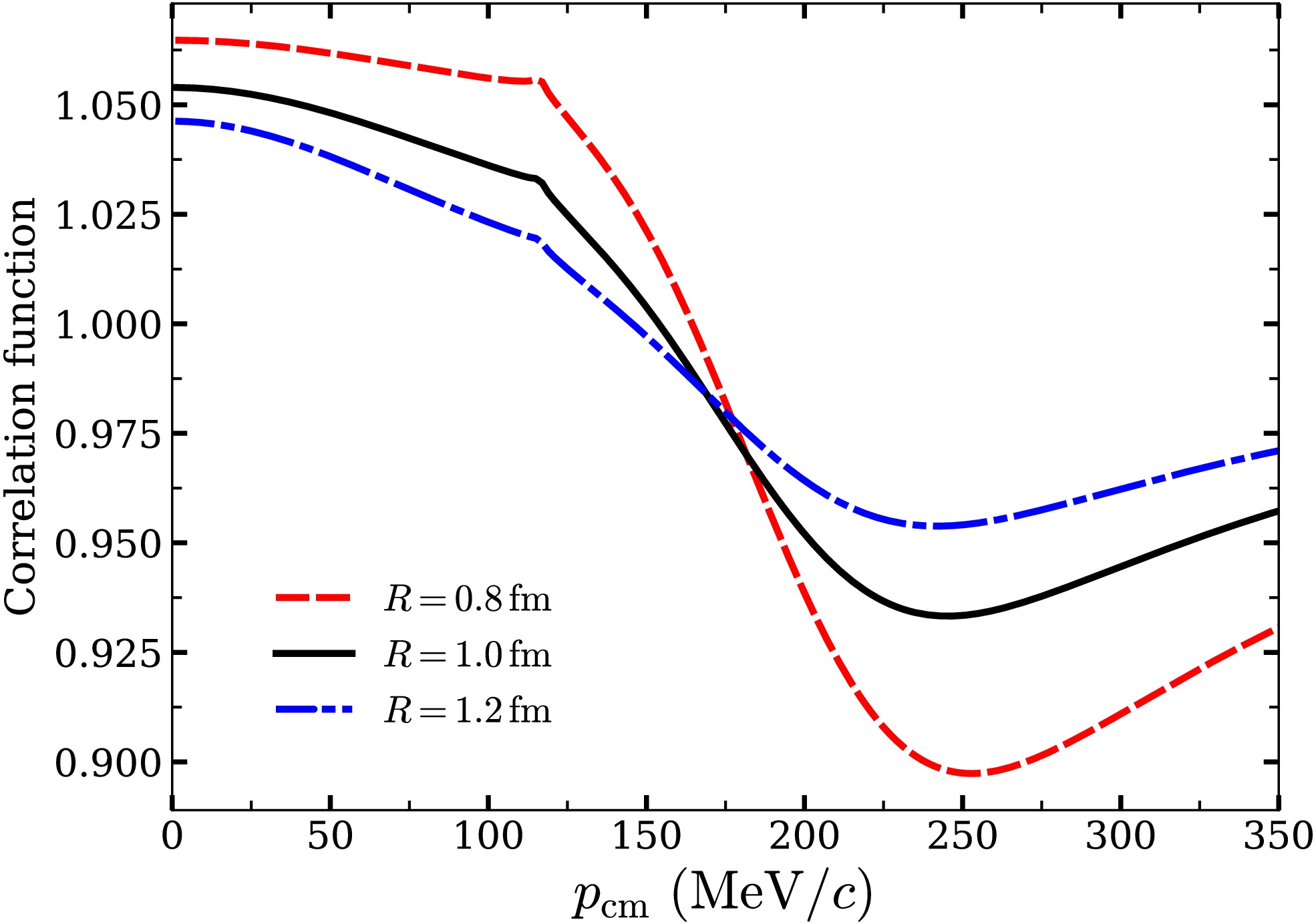
Figure 5. (color online) Correlation functions for the
$ \pi^0 f_1(1285) $ system as functions of the momentum$ p_{\rm{cm}} $ for different values of the source radius R. -
The first results we present are for the scattering length a and the effective range
$ r_0 $ . We obtain:$ a) $ for the$ \pi^0 f_1 $ system$ a = -0.05\,\mathrm{fm}, $
(28) $ r_0 = (-47.37-{\rm i}\, 0.49)\,\mathrm{fm}. $
(29) This is a special case characterized by a very small scattering length and a large effective range.
$ b) $ for the$ \eta f_1 $ system$ a = (0.29-{\rm i}\, 0.08)\,\mathrm{fm}, $
(30) $ r_0 = (0.47+{\rm i}\, 0.50)\,\mathrm{fm}. $
(31) In the latter case, the value of a is approximately half that for the
$ K f_1 $ system, and$ r_0 $ is also approximately half as large as that for the$ K f_1 $ system but has the opposite sign.Next, we show the results for the total
$ \pi^0 f_1(1285) $ amplitude as a function of$ \sqrt{s} $ in Fig. 3. In Fig. 4, we show the results for$ \eta f_1(1285) $ scattering.
Figure 3. (color online) The
$ \pi^0 f_1(1285) $ scattering amplitude$ T_{\pi^0 f_1}^{\,\mathrm{tot}} $ as a function of$ \sqrt{s} $ .
Figure 4. (color online) The
$ \eta f_1(1285) $ scattering amplitude$ T_{\eta f_1}^{\,\mathrm{tot}} $ as a function of$ \sqrt{s} $ .In Fig. 3, the
$ \pi^0 f_1(1285) $ amplitude exhibits smooth behavior at and below threshold. However, in the region$ 1500-1600 \ {\rm{ MeV}} $ , a notable structure appears. The amplitude exhibits resonance-like behavior with a phase of$ \pi/2 $ , which corresponds to having the roles of the real and imaginary parts interchanged. The modulus of the real part displays a peak, whereas the imaginary part resembles the real part of a Breit-Wigner resonance with an added constant. It is unclear whether this structure is related to the$ \pi_1(1400-1600) $ state reported in the PDG, but it is noteworthy that a structure in the amplitude emerges precisely at the energy where the$ \pi_1(1400-1600) $ has been claimed experimentally.Concerning the
$ \eta f_1 $ amplitude, we first note that we do not observe any structure around$ 1855 \ {\rm{ MeV}} $ that could be associated with the$ \eta_1(1855) $ . We can only state that we obtain a pronounced cusp structure around the threshold at$ 1830 \ {\rm{ MeV}} $ . Second, we observe some structure around$ 1500 \ {\rm{ MeV}} $ . However, this is about$ 330 \ {\rm{ MeV}} $ below the$ \eta f_1(1285) $ threshold, where we are reluctant to trust our results. We can reasonably trust our results within approximately$ 150 \ {\rm{ MeV}} $ above and below threshold, corresponding to the energy range of the correlation functions in Ref. [34]. Thus, we prefer not to make any claim concerning this structure.
Figure 6. (color online) Correlation functions for the
$ \eta f_1(1285) $ system as functions of the momentum$ p_{\rm{cm}} $ for different values of the source radius R.Next, we present the results for the correlation functions. Figure 5 shows the results for the
$ \pi^0 f_1(1285) $ correlation function. Figure 6 shows the corresponding results for the$ \eta f_1(1285) $ correlation function. For the$ \pi^0 f_1 $ case, the correlation function has values very close to$ 1 $ , indicating a weak interaction. The value of the correlation function decreases with increasing momentum at small values of$ p_{\rm{cm}} $ . The kink appearing around$ p_{\rm{cm}} \simeq 110 \ {\rm{ MeV}} $ corresponds to the opening of the$ \pi K $ threshold in the$ t_2 $ amplitude, as can be seen by applying Eq. (17), which relates s to$ s_2 $ . This corresponds to$ \sqrt{s} \simeq 1465 \ {\rm{ MeV}} $ and is also barely visible in Fig. 3 at this energy. There are no kinks related to the$ \pi K^* $ threshold because we use the convolved G functions for the$ K^* $ . In the case of the$ \eta f_1 $ interaction, the expected kink for the$ \eta K $ threshold is small and not visible in the figures. The trend of the correlation function is similar to that obtained for the$ K f_1(1285) $ case [38] but closer to unity, indicating a weaker interaction than in the$ K f_1(1285) $ case. The shape obtained is similar to that observed for$ p f_1(1285) $ in the ALICE experiment [34]; however, the strength is much weaker, with the correlation function closer to unity, than that observed in the$ p f_1(1285) $ experiment.
Figure 5. (color online) Correlation functions for the
$ \pi^0 f_1(1285) $ system as functions of the momentum$ p_{\rm{cm}} $ for different values of the source radius R. -
The first results we present are for the scattering length a and the effective range
$ r_0 $ . We obtain:$ a) $ for the$ \pi^0 f_1 $ system$ a = -0.05\,\mathrm{fm}, $
(28) $ r_0 = (-47.37-{\rm i}\, 0.49)\,\mathrm{fm}. $
(29) This is a special case characterized by a very small scattering length and a large effective range.
$ b) $ for the$ \eta f_1 $ system$ a = (0.29-{\rm i}\, 0.08)\,\mathrm{fm}, $
(30) $ r_0 = (0.47+{\rm i}\, 0.50)\,\mathrm{fm}. $
(31) In the latter case, the value of a is approximately half that for the
$ K f_1 $ system, and$ r_0 $ is also approximately half as large as that for the$ K f_1 $ system but has the opposite sign.Next, we show the results for the total
$ \pi^0 f_1(1285) $ amplitude as a function of$ \sqrt{s} $ in Fig. 3. In Fig. 4, we show the results for$ \eta f_1(1285) $ scattering.
Figure 3. (color online) The
$ \pi^0 f_1(1285) $ scattering amplitude$ T_{\pi^0 f_1}^{\,\mathrm{tot}} $ as a function of$ \sqrt{s} $ .
Figure 4. (color online) The
$ \eta f_1(1285) $ scattering amplitude$ T_{\eta f_1}^{\,\mathrm{tot}} $ as a function of$ \sqrt{s} $ .In Fig. 3, the
$ \pi^0 f_1(1285) $ amplitude exhibits smooth behavior at and below threshold. However, in the region$ 1500-1600 \ {\rm{ MeV}} $ , a notable structure appears. The amplitude exhibits resonance-like behavior with a phase of$ \pi/2 $ , which corresponds to having the roles of the real and imaginary parts interchanged. The modulus of the real part displays a peak, whereas the imaginary part resembles the real part of a Breit-Wigner resonance with an added constant. It is unclear whether this structure is related to the$ \pi_1(1400-1600) $ state reported in the PDG, but it is noteworthy that a structure in the amplitude emerges precisely at the energy where the$ \pi_1(1400-1600) $ has been claimed experimentally.Concerning the
$ \eta f_1 $ amplitude, we first note that we do not observe any structure around$ 1855 \ {\rm{ MeV}} $ that could be associated with the$ \eta_1(1855) $ . We can only state that we obtain a pronounced cusp structure around the threshold at$ 1830 \ {\rm{ MeV}} $ . Second, we observe some structure around$ 1500 \ {\rm{ MeV}} $ . However, this is about$ 330 \ {\rm{ MeV}} $ below the$ \eta f_1(1285) $ threshold, where we are reluctant to trust our results. We can reasonably trust our results within approximately$ 150 \ {\rm{ MeV}} $ above and below threshold, corresponding to the energy range of the correlation functions in Ref. [34]. Thus, we prefer not to make any claim concerning this structure.
Figure 6. (color online) Correlation functions for the
$ \eta f_1(1285) $ system as functions of the momentum$ p_{\rm{cm}} $ for different values of the source radius R.Next, we present the results for the correlation functions. Figure 5 shows the results for the
$ \pi^0 f_1(1285) $ correlation function. Figure 6 shows the corresponding results for the$ \eta f_1(1285) $ correlation function. For the$ \pi^0 f_1 $ case, the correlation function has values very close to$ 1 $ , indicating a weak interaction. The value of the correlation function decreases with increasing momentum at small values of$ p_{\rm{cm}} $ . The kink appearing around$ p_{\rm{cm}} \simeq 110 \ {\rm{ MeV}} $ corresponds to the opening of the$ \pi K $ threshold in the$ t_2 $ amplitude, as can be seen by applying Eq. (17), which relates s to$ s_2 $ . This corresponds to$ \sqrt{s} \simeq 1465 \ {\rm{ MeV}} $ and is also barely visible in Fig. 3 at this energy. There are no kinks related to the$ \pi K^* $ threshold because we use the convolved G functions for the$ K^* $ . In the case of the$ \eta f_1 $ interaction, the expected kink for the$ \eta K $ threshold is small and not visible in the figures. The trend of the correlation function is similar to that obtained for the$ K f_1(1285) $ case [38] but closer to unity, indicating a weaker interaction than in the$ K f_1(1285) $ case. The shape obtained is similar to that observed for$ p f_1(1285) $ in the ALICE experiment [34]; however, the strength is much weaker, with the correlation function closer to unity, than that observed in the$ p f_1(1285) $ experiment.
Figure 5. (color online) Correlation functions for the
$ \pi^0 f_1(1285) $ system as functions of the momentum$ p_{\rm{cm}} $ for different values of the source radius R. -
We have studied the interaction of a
$ \pi^0 $ (or η) with the$ f_1(1285) $ resonance, assuming that the$ f_1(1285) $ is a$ K^* \bar K-\bar{K^*}K $ bound state. We have used a framework analogous to calculations of an external particle interacting with a nucleus, first defining an optical potential and then constructing the Lippmann-Schwinger equation from it. In our case, the role of the nucleus is played by the two-particle cluster, the$ f_1(1285) $ , while the external particle is either a$ \pi^0 $ or an η. The optical potential is obtained using the formalism of the fixed center approximation (FCA) to the three-body Faddeev equations. The main assumption is that the two-particle cluster remains intact during the interaction, a situation well suited to the present case, where the$ f_1(1285) $ particle appears both at the beginning and at the end of the interaction.The study of this interaction becomes more relevant when compared with other calculations in which the kernel of the
$ \pi^0 (\eta)\, f_1(1285) $ interaction is obtained by treating the$ f_1(1285) $ as a matter source and using the Weinberg-Tomozawa interaction, which vanishes in these two cases. We have shown that, in our case, we go beyond the$ O(1/f^2) $ level of the Weinberg-Tomozawa interaction. Our total amplitudes use as input individual$ t_i $ matrices that contain terms beyond$ O(1/f^2) $ , obtained from coupled-channel calculations that implement coupled-channel unitarity, and these amplitudes do not vanish.We have calculated the total amplitudes for the
$ \pi^0 (\eta)\, f_1(1285) $ interaction and find no clear signals for the$ \pi_1(1400) $ ,$ \pi_1(1600) $ , or$ \eta_1(1855) $ resonances within our approach. However, we observe a weak structure around$ 1500-1600 \ {\rm{ MeV}} $ in the$ \pi^0 f_1(1285) $ amplitude, and a strong cusp structure in the$ \eta f_1(1285) $ amplitude at the$ \eta f_1(1285) $ threshold around$ 1830 \ {\rm{ MeV}} $ .We should mention that, in Ref. [26], despite the vanishing
$ \pi^0 (\eta)\, f_1(1285) $ interaction, the use of coupled channels involving other pseudoscalar meson–axial-vector meson channels ultimately leads to the$ \pi_1(1600) $ and$ \eta_1(1855) $ states. In our case, such an extension would in principle be possible; however, rather than dealing with the overlap of two particles in the framework of Ref. [26], we would have to deal with the overlap of three particles in this hypothetical calculation, since the axial-vector mesons are molecular states in our approach. We consider this three-body overlap to be more difficult than in the two-body case. Thus, we do not anticipate a significant effect from this hypothetical calculation. This renders the theoretical explanation of the$ \pi_1(1600) $ and$ \eta_1(1855) $ states more challenging than previously assumed.Regarding Ref. [13], the authors reported obtaining the
$ \pi_1(1600) $ from the$ \pi f_1(1285) $ interaction using the FCA. It is unclear whether the structure that we find for the$ \pi^0 f_1(1285) $ amplitude around$ 1500-1600 \ {\rm{ MeV}} $ is related to the state found in Ref. [13]. There are some differences between our approach and that of Ref. [13], since we use the new formalism that implements elastic unitarity in the FCA amplitude. As previously discussed, the standard FCA amplitude does not satisfy unitarity at threshold; hence, it cannot be reliably used near threshold and becomes more uncertain further above it. This problem was already anticipated when comparing the FCA results with a Faddeev calculation for a state appearing above threshold, the$ \phi(2170) $ , where the failure of the FCA in that case could be observed [54].In the present work, we have evaluated the scattering length and effective range for the
$ \pi^0 (\eta)\, f_1(1285) $ interaction, as well as the corresponding correlation functions. With the advent of the first experimental measurement of the correlation function for a proton and the$ f_1(1285) $ , a door has been opened for future studies of the interaction of other particles with the$ f_1(1285) $ and with other resonances. It will be interesting to compare these predictions with the experimental results. The good agreement between the predictions obtained using the present formalism for the interaction of a proton and the$ f_1(1285) $ in Ref. [40] and subsequent experimental results [34] makes us optimistic about the outcome of these comparisons. -
We have studied the interaction of a
$ \pi^0 $ (or η) with the$ f_1(1285) $ resonance, assuming that the$ f_1(1285) $ is a$ K^* \bar K-\bar{K^*}K $ bound state. We have used a framework analogous to calculations of an external particle interacting with a nucleus, first defining an optical potential and then constructing the Lippmann-Schwinger equation from it. In our case, the role of the nucleus is played by the two-particle cluster, the$ f_1(1285) $ , while the external particle is either a$ \pi^0 $ or an η. The optical potential is obtained using the formalism of the fixed center approximation (FCA) to the three-body Faddeev equations. The main assumption is that the two-particle cluster remains intact during the interaction, a situation well suited to the present case, where the$ f_1(1285) $ particle appears both at the beginning and at the end of the interaction.The study of this interaction becomes more relevant when compared with other calculations in which the kernel of the
$ \pi^0 (\eta)\, f_1(1285) $ interaction is obtained by treating the$ f_1(1285) $ as a matter source and using the Weinberg-Tomozawa interaction, which vanishes in these two cases. We have shown that, in our case, we go beyond the$ O(1/f^2) $ level of the Weinberg-Tomozawa interaction. Our total amplitudes use as input individual$ t_i $ matrices that contain terms beyond$ O(1/f^2) $ , obtained from coupled-channel calculations that implement coupled-channel unitarity, and these amplitudes do not vanish.We have calculated the total amplitudes for the
$ \pi^0 (\eta)\, f_1(1285) $ interaction and find no clear signals for the$ \pi_1(1400) $ ,$ \pi_1(1600) $ , or$ \eta_1(1855) $ resonances within our approach. However, we observe a weak structure around$ 1500-1600 \ {\rm{ MeV}} $ in the$ \pi^0 f_1(1285) $ amplitude, and a strong cusp structure in the$ \eta f_1(1285) $ amplitude at the$ \eta f_1(1285) $ threshold around$ 1830 \ {\rm{ MeV}} $ .We should mention that, in Ref. [26], despite the vanishing
$ \pi^0 (\eta)\, f_1(1285) $ interaction, the use of coupled channels involving other pseudoscalar meson–axial-vector meson channels ultimately leads to the$ \pi_1(1600) $ and$ \eta_1(1855) $ states. In our case, such an extension would in principle be possible; however, rather than dealing with the overlap of two particles in the framework of Ref. [26], we would have to deal with the overlap of three particles in this hypothetical calculation, since the axial-vector mesons are molecular states in our approach. We consider this three-body overlap to be more difficult than in the two-body case. Thus, we do not anticipate a significant effect from this hypothetical calculation. This renders the theoretical explanation of the$ \pi_1(1600) $ and$ \eta_1(1855) $ states more challenging than previously assumed.Regarding Ref. [13], the authors reported obtaining the
$ \pi_1(1600) $ from the$ \pi f_1(1285) $ interaction using the FCA. It is unclear whether the structure that we find for the$ \pi^0 f_1(1285) $ amplitude around$ 1500-1600 \ {\rm{ MeV}} $ is related to the state found in Ref. [13]. There are some differences between our approach and that of Ref. [13], since we use the new formalism that implements elastic unitarity in the FCA amplitude. As previously discussed, the standard FCA amplitude does not satisfy unitarity at threshold; hence, it cannot be reliably used near threshold and becomes more uncertain further above it. This problem was already anticipated when comparing the FCA results with a Faddeev calculation for a state appearing above threshold, the$ \phi(2170) $ , where the failure of the FCA in that case could be observed [54].In the present work, we have evaluated the scattering length and effective range for the
$ \pi^0 (\eta)\, f_1(1285) $ interaction, as well as the corresponding correlation functions. With the advent of the first experimental measurement of the correlation function for a proton and the$ f_1(1285) $ , a door has been opened for future studies of the interaction of other particles with the$ f_1(1285) $ and with other resonances. It will be interesting to compare these predictions with the experimental results. The good agreement between the predictions obtained using the present formalism for the interaction of a proton and the$ f_1(1285) $ in Ref. [40] and subsequent experimental results [34] makes us optimistic about the outcome of these comparisons. -
We have studied the interaction of a
$ \pi^0 $ (or η) with the$ f_1(1285) $ resonance, assuming that the$ f_1(1285) $ is a$ K^* \bar K-\bar{K^*}K $ bound state. We have used a framework analogous to calculations of an external particle interacting with a nucleus, first defining an optical potential and then constructing the Lippmann-Schwinger equation from it. In our case, the role of the nucleus is played by the two-particle cluster, the$ f_1(1285) $ , while the external particle is either a$ \pi^0 $ or an η. The optical potential is obtained using the formalism of the fixed center approximation (FCA) to the three-body Faddeev equations. The main assumption is that the two-particle cluster remains intact during the interaction, a situation well suited to the present case, where the$ f_1(1285) $ particle appears both at the beginning and at the end of the interaction.The study of this interaction becomes more relevant when compared with other calculations in which the kernel of the
$ \pi^0 (\eta)\, f_1(1285) $ interaction is obtained by treating the$ f_1(1285) $ as a matter source and using the Weinberg-Tomozawa interaction, which vanishes in these two cases. We have shown that, in our case, we go beyond the$ O(1/f^2) $ level of the Weinberg-Tomozawa interaction. Our total amplitudes use as input individual$ t_i $ matrices that contain terms beyond$ O(1/f^2) $ , obtained from coupled-channel calculations that implement coupled-channel unitarity, and these amplitudes do not vanish.We have calculated the total amplitudes for the
$ \pi^0 (\eta)\, f_1(1285) $ interaction and find no clear signals for the$ \pi_1(1400) $ ,$ \pi_1(1600) $ , or$ \eta_1(1855) $ resonances within our approach. However, we observe a weak structure around$ 1500-1600 \ {\rm{ MeV}} $ in the$ \pi^0 f_1(1285) $ amplitude, and a strong cusp structure in the$ \eta f_1(1285) $ amplitude at the$ \eta f_1(1285) $ threshold around$ 1830 \ {\rm{ MeV}} $ .We should mention that, in Ref. [26], despite the vanishing
$ \pi^0 (\eta)\, f_1(1285) $ interaction, the use of coupled channels involving other pseudoscalar meson–axial-vector meson channels ultimately leads to the$ \pi_1(1600) $ and$ \eta_1(1855) $ states. In our case, such an extension would in principle be possible; however, rather than dealing with the overlap of two particles in the framework of Ref. [26], we would have to deal with the overlap of three particles in this hypothetical calculation, since the axial-vector mesons are molecular states in our approach. We consider this three-body overlap to be more difficult than in the two-body case. Thus, we do not anticipate a significant effect from this hypothetical calculation. This renders the theoretical explanation of the$ \pi_1(1600) $ and$ \eta_1(1855) $ states more challenging than previously assumed.Regarding Ref. [13], the authors reported obtaining the
$ \pi_1(1600) $ from the$ \pi f_1(1285) $ interaction using the FCA. It is unclear whether the structure that we find for the$ \pi^0 f_1(1285) $ amplitude around$ 1500-1600 \ {\rm{ MeV}} $ is related to the state found in Ref. [13]. There are some differences between our approach and that of Ref. [13], since we use the new formalism that implements elastic unitarity in the FCA amplitude. As previously discussed, the standard FCA amplitude does not satisfy unitarity at threshold; hence, it cannot be reliably used near threshold and becomes more uncertain further above it. This problem was already anticipated when comparing the FCA results with a Faddeev calculation for a state appearing above threshold, the$ \phi(2170) $ , where the failure of the FCA in that case could be observed [54].In the present work, we have evaluated the scattering length and effective range for the
$ \pi^0 (\eta)\, f_1(1285) $ interaction, as well as the corresponding correlation functions. With the advent of the first experimental measurement of the correlation function for a proton and the$ f_1(1285) $ , a door has been opened for future studies of the interaction of other particles with the$ f_1(1285) $ and with other resonances. It will be interesting to compare these predictions with the experimental results. The good agreement between the predictions obtained using the present formalism for the interaction of a proton and the$ f_1(1285) $ in Ref. [40] and subsequent experimental results [34] makes us optimistic about the outcome of these comparisons. -
As shown in Appendix A, the required amplitudes are obtained using the chiral unitary approach in coupled channels, with the transition potential derived from chiral Lagrangians at lowest order. Possible contributions from higher-order potentials are empirically accommodated through the choice of
$ q_{\mathrm{max}} $ , which is fitted to scattering data or to the masses of the generated resonances. For a single channel, and for simplicity of the argument, one has$ t=[V^{-1}-G]^{-1} $ ; hence, changes in V can be accommodated by modifying the G function through the cutoff$ q_{\mathrm{max}} $ in the loop integration. We used$ q_{\mathrm{max}}=600 \ {\rm{ MeV}} $ to evaluate the relevant scattering matrices in Appendix A, and we examine the stability of the results under reasonable variations of$ q_{\mathrm{max}} $ .The same considerations that apply to the scattering matrices
$ t_1 $ and$ t_2 $ also apply to the wave function of the cluster in Eq. (9). In Ref. [28], the value of$ q_{\mathrm{max}} $ used to generate the different axial-vector resonances was$ q_{\mathrm{max}} \simeq 1000 \ {\rm{ MeV}} $ , and the mass of the$ f_1(1285) $ was predicted to be quite close to the physical value. Here, by tuning$ q_{\mathrm{max}} $ to reproduce the exact mass of the$ f_1(1285) $ , we obtain$ q_{\mathrm{max}}=971.5 \ {\rm{ MeV}} $ . We then test the stability of the results by varying$ q_{\mathrm{max}} $ upward and downward by$ 10$ %. The resulting changes in the scattering length and effective range of$ \pi^0 f_1(1285) $ are well below$ 1$ %. The changes are larger for the$ \eta f_1(1285) $ system: approximately$ 2$ % for the scattering length and up to$ 15$ % for the effective range. The changes in the correlation functions for both systems are very small and are much smaller than those induced by varying$ q_{\mathrm{max}} $ in the evaluation of$ t_1 $ and$ t_2 $ , as shown below.The large value of
$ r_0 $ in the$ \pi^0 f_1(1285) $ system, approximately 47 fm, appears abnormally large. One might expect this value to change if the width of the$ f_1(1285) $ , which has been neglected thus far, is included. We can include this width by performing a convolution of the results with the spectral function of the$ f_1(1285) $ resonance,$ S(M_{\mathrm{inv}}) = - \dfrac{1}{\pi} \mathrm{Im} \dfrac{1}{M_{\mathrm{inv}}^2 - M_{f_1}^2 + {\rm i} M_{f_1} \Gamma_{f_1}} $ , as in the study of the$ K f_1(1285) $ system [38]. The changes in a and$ r_0 $ for the$ \pi^0 f_1(1285) $ system are small. The values obtained after the convolution are$ a = -0.05\;\mathrm{fm}, $
(32) $ r_0 = (-50.38-{\rm i}\, 0.34)\;\mathrm{fm}. $
(33) Thus, a remains unchanged, whereas
$ r_0 $ changes by$ 6$ %. This indicates that the convolution with the$ f_1(1285) $ width does not alter the large value of the effective range. To understand the large value of$ r_0 $ , we refer to Eq. (21) and Fig. 3. Numerically, the structure found above threshold requires a small value of a and a large value of$ r_0 $ to be reproduced.We also find that the changes in the amplitude and correlation function of
$ \pi^0 f_1(1285) $ induced by the convolution are small, and are much smaller than those generated by variations of$ q_{\mathrm{max}} $ in$ t_1 $ and$ t_2 $ , as shown below.The changes in the
$ \eta f_1(1285) $ observables are larger than those found previously. We now obtain$ a = (0.30-{\rm i}\, 0.10)\;\mathrm{fm}, $
(34) $ r_0 = (-1.46+{\rm i}\, 0.57)\;\mathrm{fm}. $
(35) A comparison with the results of Eqs. (30) and (31) shows that the changes in a are moderate; however, the value of
$ r_0 $ changes substantially and even changes sign. It is also informative to examine how the scattering amplitude and the correlation function change. We show these effects in Fig. 7 for the three-body amplitude and in Fig. 8 for the correlation function. The changes are moderate, but the amplitude softens at threshold, and the correlation function exhibits small changes at very small values of$ p_{\mathrm{cm}} $ .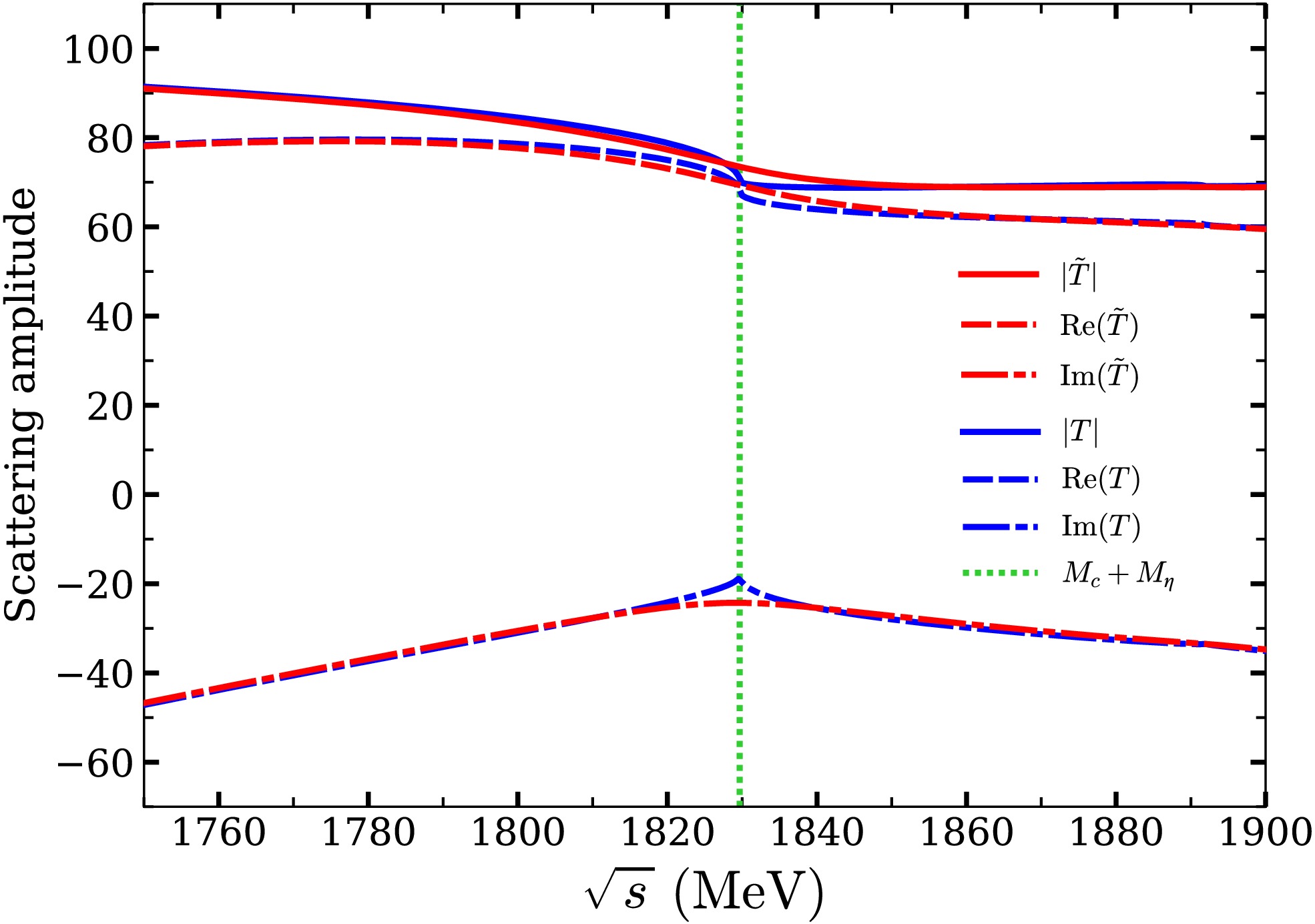
Figure 7. (color online) Changes in the scattering amplitude induced by the convolution accounting for the
$ f_1(1285) $ width.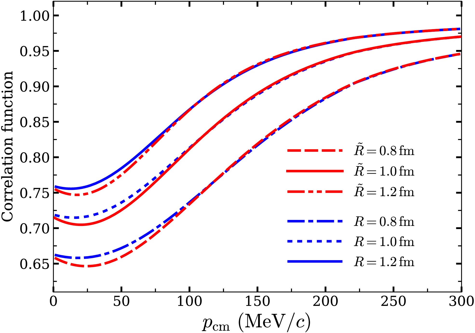
Figure 8. (color online) Changes in the correlation function induced by convolution with the
$ f_1(1285) $ width.The largest changes, which remain moderate, arise from varying
$ q_{\mathrm{max}} $ in the$ \pi K $ amplitudes. Following Ref. [55], we assume that a$ 10$ % change in the$ \pi K $ potential can be compensated by a corresponding$ 10$ % increase or decrease in$ q_{\mathrm{max}} $ (starting from$ q_{\mathrm{max}}=600 \ {\rm{ MeV}} $ ) in order to keep the$ K_0^*(700) $ position fixed. We then obtain a band of values$ {\rm{i)}} $ $ \pi^0 f_1(1285) $ :$ \begin{split} &a \in [-0.04, -0.05] \;\text{fm}, \\& r_0 \in [-45.63 -{\rm i} 0.62, -47.14 - {\rm i} 0.41] \;\text{fm}; \end{split} $
(36) $ {\rm{ii)}} $ $ \eta f_1(1285) $ :$ \begin{split} & a \in [0.27-{\rm i}0.08,\,0.32-{\rm i}0.07]\;\mathrm{fm}, \\ & r_0 \in [0.37 + {\rm i}\, 0.47,\,0.65 + {\rm i}\, 0.53]\;\mathrm{fm}. \end{split} $
(37) In Figs. 9−12, we show the bands of values obtained for the three-body amplitude and the correlation function for the
$ \pi^0 f_1(1285) $ and$ \eta f_1(1285) $ systems. The bands exhibit larger uncertainties than those from the sources discussed previously, but they remain moderate and do not alter the basic structure or characteristics of the calculated observables.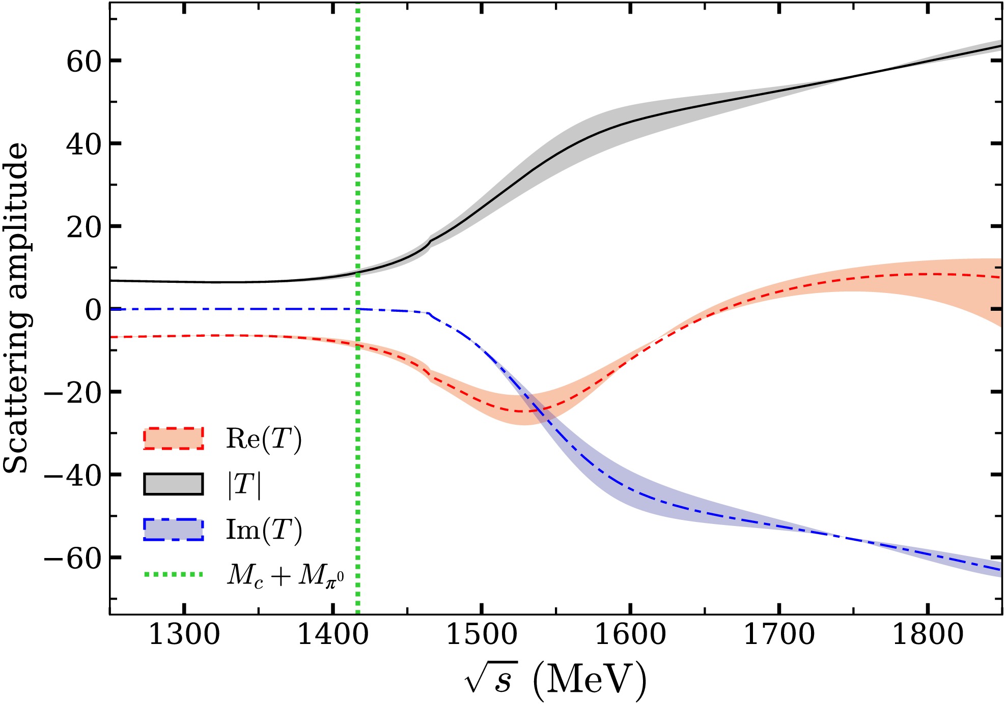
Figure 9. (color online) Range of values for the
$ \pi^0 f_1(1285) $ three-body amplitudes arising from uncertainties in the$ \pi K $ amplitude.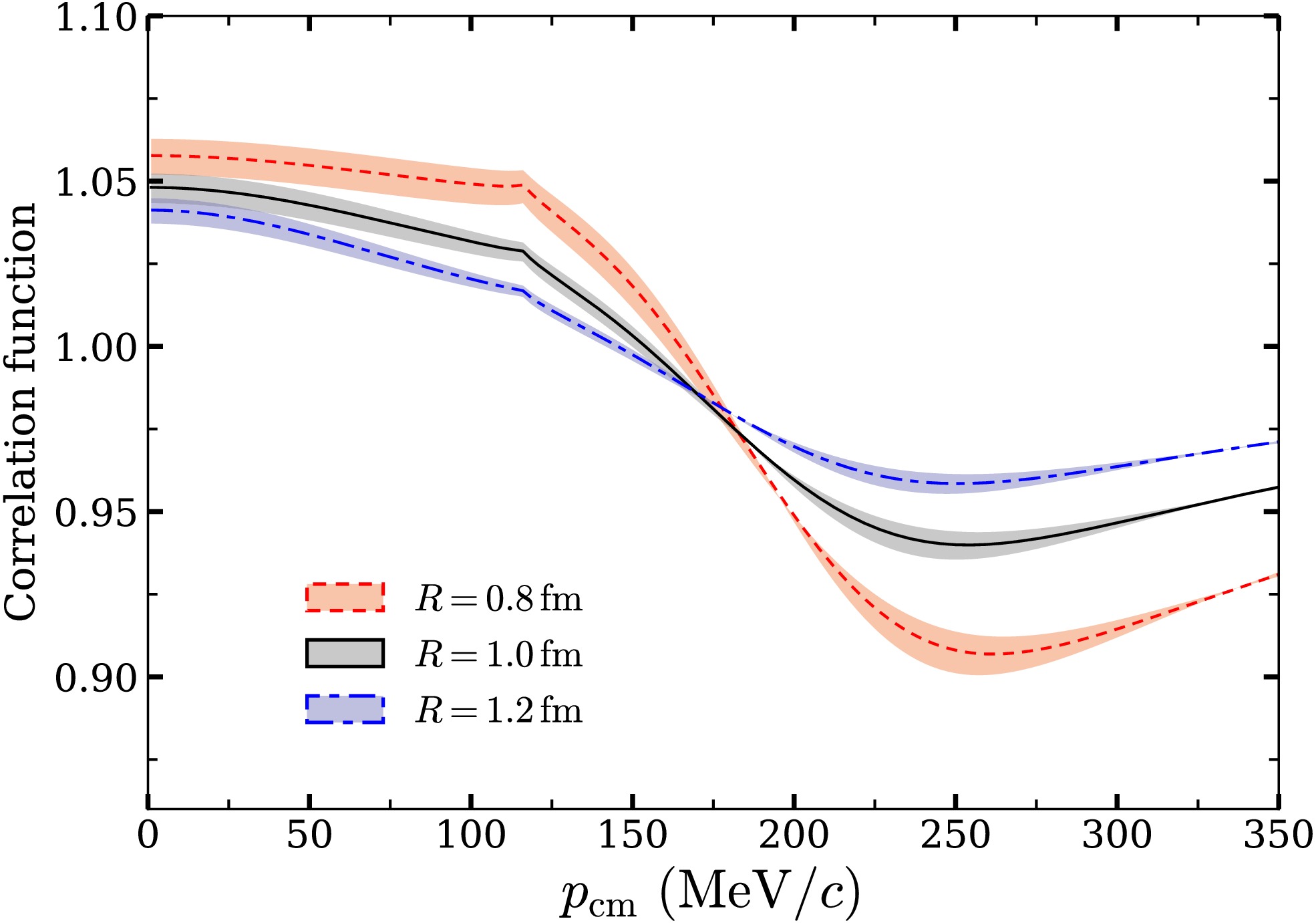
Figure 10. (color online) Uncertainty band for the
$ \pi^0 f_1(1285) $ correlation function arising from uncertainties in the$ \pi K $ amplitude.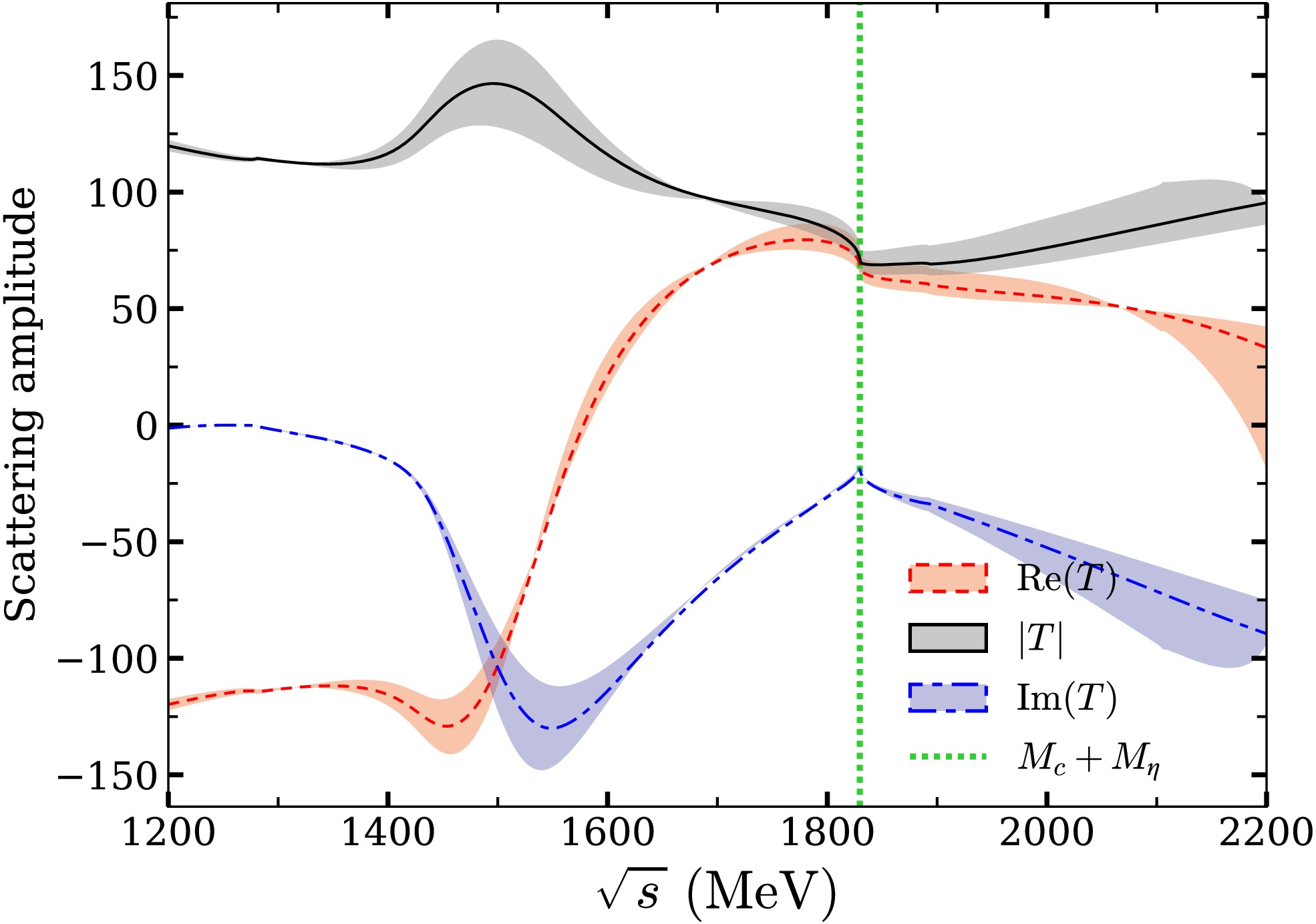
Figure 11. (color online) Range of values for the
$ \eta f_1(1285) $ amplitude arising from uncertainties in the$ \pi K $ amplitude.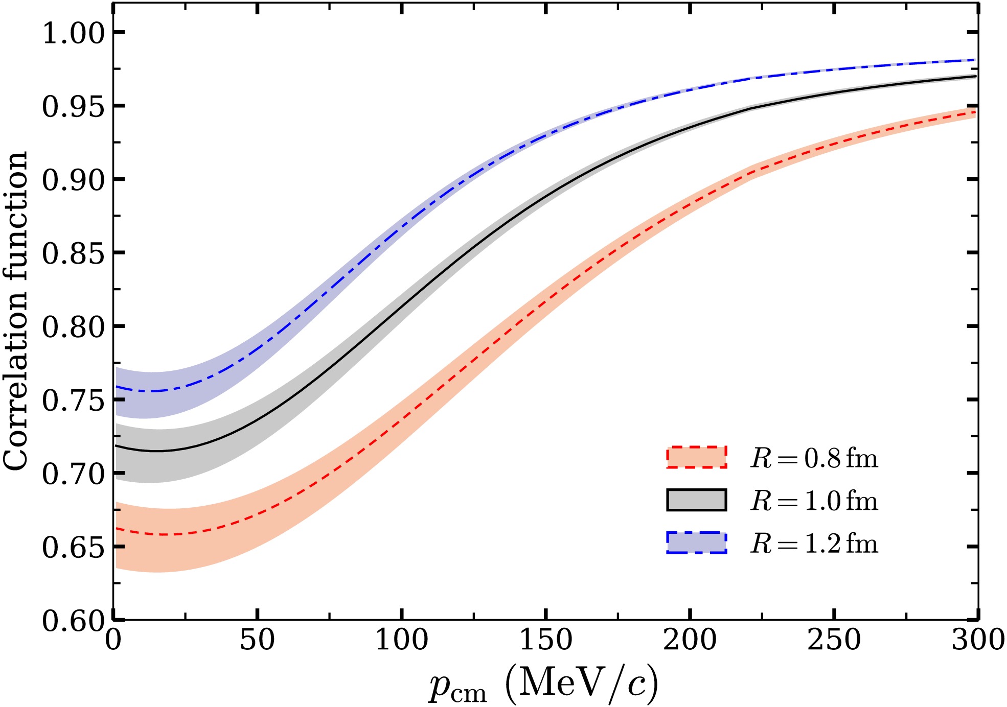
Figure 12. (color online) Range of values for the
$ \eta f_1(1285) $ correlation function arising from uncertainties in the$ \pi K $ amplitude. -
As shown in Appendix A, the required amplitudes are obtained using the chiral unitary approach in coupled channels, with the transition potential derived from chiral Lagrangians at lowest order. Possible contributions from higher-order potentials are empirically accommodated through the choice of
$ q_{\mathrm{max}} $ , which is fitted to scattering data or to the masses of the generated resonances. For a single channel, and for simplicity of the argument, one has$ t=[V^{-1}-G]^{-1} $ ; hence, changes in V can be accommodated by modifying the G function through the cutoff$ q_{\mathrm{max}} $ in the loop integration. We used$ q_{\mathrm{max}}=600 \ {\rm{ MeV}} $ to evaluate the relevant scattering matrices in Appendix A, and we examine the stability of the results under reasonable variations of$ q_{\mathrm{max}} $ .The same considerations that apply to the scattering matrices
$ t_1 $ and$ t_2 $ also apply to the wave function of the cluster in Eq. (9). In Ref. [28], the value of$ q_{\mathrm{max}} $ used to generate the different axial-vector resonances was$ q_{\mathrm{max}} \simeq 1000 \ {\rm{ MeV}} $ , and the mass of the$ f_1(1285) $ was predicted to be quite close to the physical value. Here, by tuning$ q_{\mathrm{max}} $ to reproduce the exact mass of the$ f_1(1285) $ , we obtain$ q_{\mathrm{max}}=971.5 \ {\rm{ MeV}} $ . We then test the stability of the results by varying$ q_{\mathrm{max}} $ upward and downward by$ 10$ %. The resulting changes in the scattering length and effective range of$ \pi^0 f_1(1285) $ are well below$ 1$ %. The changes are larger for the$ \eta f_1(1285) $ system: approximately$ 2$ % for the scattering length and up to$ 15$ % for the effective range. The changes in the correlation functions for both systems are very small and are much smaller than those induced by varying$ q_{\mathrm{max}} $ in the evaluation of$ t_1 $ and$ t_2 $ , as shown below.The large value of
$ r_0 $ in the$ \pi^0 f_1(1285) $ system, approximately 47 fm, appears abnormally large. One might expect this value to change if the width of the$ f_1(1285) $ , which has been neglected thus far, is included. We can include this width by performing a convolution of the results with the spectral function of the$ f_1(1285) $ resonance,$ S(M_{\mathrm{inv}}) = - \dfrac{1}{\pi} \mathrm{Im} \dfrac{1}{M_{\mathrm{inv}}^2 - M_{f_1}^2 + {\rm i} M_{f_1} \Gamma_{f_1}} $ , as in the study of the$ K f_1(1285) $ system [38]. The changes in a and$ r_0 $ for the$ \pi^0 f_1(1285) $ system are small. The values obtained after the convolution are$ a = -0.05\;\mathrm{fm}, $
(32) $ r_0 = (-50.38-{\rm i}\, 0.34)\;\mathrm{fm}. $
(33) Thus, a remains unchanged, whereas
$ r_0 $ changes by$ 6$ %. This indicates that the convolution with the$ f_1(1285) $ width does not alter the large value of the effective range. To understand the large value of$ r_0 $ , we refer to Eq. (21) and Fig. 3. Numerically, the structure found above threshold requires a small value of a and a large value of$ r_0 $ to be reproduced.We also find that the changes in the amplitude and correlation function of
$ \pi^0 f_1(1285) $ induced by the convolution are small, and are much smaller than those generated by variations of$ q_{\mathrm{max}} $ in$ t_1 $ and$ t_2 $ , as shown below.The changes in the
$ \eta f_1(1285) $ observables are larger than those found previously. We now obtain$ a = (0.30-{\rm i}\, 0.10)\;\mathrm{fm}, $
(34) $ r_0 = (-1.46+{\rm i}\, 0.57)\;\mathrm{fm}. $
(35) A comparison with the results of Eqs. (30) and (31) shows that the changes in a are moderate; however, the value of
$ r_0 $ changes substantially and even changes sign. It is also informative to examine how the scattering amplitude and the correlation function change. We show these effects in Fig. 7 for the three-body amplitude and in Fig. 8 for the correlation function. The changes are moderate, but the amplitude softens at threshold, and the correlation function exhibits small changes at very small values of$ p_{\mathrm{cm}} $ .
Figure 7. (color online) Changes in the scattering amplitude induced by the convolution accounting for the
$ f_1(1285) $ width.
Figure 8. (color online) Changes in the correlation function induced by convolution with the
$ f_1(1285) $ width.The largest changes, which remain moderate, arise from varying
$ q_{\mathrm{max}} $ in the$ \pi K $ amplitudes. Following Ref. [55], we assume that a$ 10$ % change in the$ \pi K $ potential can be compensated by a corresponding$ 10$ % increase or decrease in$ q_{\mathrm{max}} $ (starting from$ q_{\mathrm{max}}=600 \ {\rm{ MeV}} $ ) in order to keep the$ K_0^*(700) $ position fixed. We then obtain a band of values$ {\rm{i)}} $ $ \pi^0 f_1(1285) $ :$ \begin{split} &a \in [-0.04, -0.05] \;\text{fm}, \\& r_0 \in [-45.63 -{\rm i} 0.62, -47.14 - {\rm i} 0.41] \;\text{fm}; \end{split} $
(36) $ {\rm{ii)}} $ $ \eta f_1(1285) $ :$ \begin{split} & a \in [0.27-{\rm i}0.08,\,0.32-{\rm i}0.07]\;\mathrm{fm}, \\ & r_0 \in [0.37 + {\rm i}\, 0.47,\,0.65 + {\rm i}\, 0.53]\;\mathrm{fm}. \end{split} $
(37) In Figs. 9−12, we show the bands of values obtained for the three-body amplitude and the correlation function for the
$ \pi^0 f_1(1285) $ and$ \eta f_1(1285) $ systems. The bands exhibit larger uncertainties than those from the sources discussed previously, but they remain moderate and do not alter the basic structure or characteristics of the calculated observables.
Figure 9. (color online) Range of values for the
$ \pi^0 f_1(1285) $ three-body amplitudes arising from uncertainties in the$ \pi K $ amplitude.
Figure 10. (color online) Uncertainty band for the
$ \pi^0 f_1(1285) $ correlation function arising from uncertainties in the$ \pi K $ amplitude.
Figure 11. (color online) Range of values for the
$ \eta f_1(1285) $ amplitude arising from uncertainties in the$ \pi K $ amplitude.
Figure 12. (color online) Range of values for the
$ \eta f_1(1285) $ correlation function arising from uncertainties in the$ \pi K $ amplitude. -
As shown in Appendix A, the required amplitudes are obtained using the chiral unitary approach in coupled channels, with the transition potential derived from chiral Lagrangians at lowest order. Possible contributions from higher-order potentials are empirically accommodated through the choice of
$ q_{\mathrm{max}} $ , which is fitted to scattering data or to the masses of the generated resonances. For a single channel, and for simplicity of the argument, one has$ t=[V^{-1}-G]^{-1} $ ; hence, changes in V can be accommodated by modifying the G function through the cutoff$ q_{\mathrm{max}} $ in the loop integration. We used$ q_{\mathrm{max}}=600 \ {\rm{ MeV}} $ to evaluate the relevant scattering matrices in Appendix A, and we examine the stability of the results under reasonable variations of$ q_{\mathrm{max}} $ .The same considerations that apply to the scattering matrices
$ t_1 $ and$ t_2 $ also apply to the wave function of the cluster in Eq. (9). In Ref. [28], the value of$ q_{\mathrm{max}} $ used to generate the different axial-vector resonances was$ q_{\mathrm{max}} \simeq 1000 \ {\rm{ MeV}} $ , and the mass of the$ f_1(1285) $ was predicted to be quite close to the physical value. Here, by tuning$ q_{\mathrm{max}} $ to reproduce the exact mass of the$ f_1(1285) $ , we obtain$ q_{\mathrm{max}}=971.5 \ {\rm{ MeV}} $ . We then test the stability of the results by varying$ q_{\mathrm{max}} $ upward and downward by$ 10$ %. The resulting changes in the scattering length and effective range of$ \pi^0 f_1(1285) $ are well below$ 1$ %. The changes are larger for the$ \eta f_1(1285) $ system: approximately$ 2$ % for the scattering length and up to$ 15$ % for the effective range. The changes in the correlation functions for both systems are very small and are much smaller than those induced by varying$ q_{\mathrm{max}} $ in the evaluation of$ t_1 $ and$ t_2 $ , as shown below.The large value of
$ r_0 $ in the$ \pi^0 f_1(1285) $ system, approximately 47 fm, appears abnormally large. One might expect this value to change if the width of the$ f_1(1285) $ , which has been neglected thus far, is included. We can include this width by performing a convolution of the results with the spectral function of the$ f_1(1285) $ resonance,$ S(M_{\mathrm{inv}}) = - \dfrac{1}{\pi} \mathrm{Im} \dfrac{1}{M_{\mathrm{inv}}^2 - M_{f_1}^2 + {\rm i} M_{f_1} \Gamma_{f_1}} $ , as in the study of the$ K f_1(1285) $ system [38]. The changes in a and$ r_0 $ for the$ \pi^0 f_1(1285) $ system are small. The values obtained after the convolution are$ a = -0.05\;\mathrm{fm}, $
(32) $ r_0 = (-50.38-{\rm i}\, 0.34)\;\mathrm{fm}. $
(33) Thus, a remains unchanged, whereas
$ r_0 $ changes by$ 6$ %. This indicates that the convolution with the$ f_1(1285) $ width does not alter the large value of the effective range. To understand the large value of$ r_0 $ , we refer to Eq. (21) and Fig. 3. Numerically, the structure found above threshold requires a small value of a and a large value of$ r_0 $ to be reproduced.We also find that the changes in the amplitude and correlation function of
$ \pi^0 f_1(1285) $ induced by the convolution are small, and are much smaller than those generated by variations of$ q_{\mathrm{max}} $ in$ t_1 $ and$ t_2 $ , as shown below.The changes in the
$ \eta f_1(1285) $ observables are larger than those found previously. We now obtain$ a = (0.30-{\rm i}\, 0.10)\;\mathrm{fm}, $
(34) $ r_0 = (-1.46+{\rm i}\, 0.57)\;\mathrm{fm}. $
(35) A comparison with the results of Eqs. (30) and (31) shows that the changes in a are moderate; however, the value of
$ r_0 $ changes substantially and even changes sign. It is also informative to examine how the scattering amplitude and the correlation function change. We show these effects in Fig. 7 for the three-body amplitude and in Fig. 8 for the correlation function. The changes are moderate, but the amplitude softens at threshold, and the correlation function exhibits small changes at very small values of$ p_{\mathrm{cm}} $ .
Figure 7. (color online) Changes in the scattering amplitude induced by the convolution accounting for the
$ f_1(1285) $ width.
Figure 8. (color online) Changes in the correlation function induced by convolution with the
$ f_1(1285) $ width.The largest changes, which remain moderate, arise from varying
$ q_{\mathrm{max}} $ in the$ \pi K $ amplitudes. Following Ref. [55], we assume that a$ 10$ % change in the$ \pi K $ potential can be compensated by a corresponding$ 10$ % increase or decrease in$ q_{\mathrm{max}} $ (starting from$ q_{\mathrm{max}}=600 \ {\rm{ MeV}} $ ) in order to keep the$ K_0^*(700) $ position fixed. We then obtain a band of values$ {\rm{i)}} $ $ \pi^0 f_1(1285) $ :$ \begin{split} &a \in [-0.04, -0.05] \;\text{fm}, \\& r_0 \in [-45.63 -{\rm i} 0.62, -47.14 - {\rm i} 0.41] \;\text{fm}; \end{split} $
(36) $ {\rm{ii)}} $ $ \eta f_1(1285) $ :$ \begin{split} & a \in [0.27-{\rm i}0.08,\,0.32-{\rm i}0.07]\;\mathrm{fm}, \\ & r_0 \in [0.37 + {\rm i}\, 0.47,\,0.65 + {\rm i}\, 0.53]\;\mathrm{fm}. \end{split} $
(37) In Figs. 9−12, we show the bands of values obtained for the three-body amplitude and the correlation function for the
$ \pi^0 f_1(1285) $ and$ \eta f_1(1285) $ systems. The bands exhibit larger uncertainties than those from the sources discussed previously, but they remain moderate and do not alter the basic structure or characteristics of the calculated observables.
Figure 9. (color online) Range of values for the
$ \pi^0 f_1(1285) $ three-body amplitudes arising from uncertainties in the$ \pi K $ amplitude.
Figure 10. (color online) Uncertainty band for the
$ \pi^0 f_1(1285) $ correlation function arising from uncertainties in the$ \pi K $ amplitude.
Figure 11. (color online) Range of values for the
$ \eta f_1(1285) $ amplitude arising from uncertainties in the$ \pi K $ amplitude.
Figure 12. (color online) Range of values for the
$ \eta f_1(1285) $ correlation function arising from uncertainties in the$ \pi K $ amplitude. -
For the
$ \pi^0 f_1(1285) $ system, we require the amplitudes$ t_{\pi K^{*}}^{I=3/2} $ ,$ t_{\pi K^{*}}^{I=1/2} $ ,$ t_{\pi K}^{I=3/2} $ , and$ t_{\pi K}^{I=1/2} $ , which appear in$ t_1,\, t_2 $ of Eq. (3).We first evaluate the amplitudes for
$ \pi^0 \bar K $ scattering. Owing to charge conjugation symmetry, the$ \pi \bar{K} $ interaction is equivalent to the$ \pi K $ interaction.We adopt the framework developed in Ref. [55], which considers the interactions among the
$ \pi^- K^+ $ ,$ \pi^0 K^0 $ , and$ \eta K^0 $ coupled channels. In this approach, the corresponding transition potentials$ V_{ij} $ are summarized in Table A1, where$ f=93 \ {\rm{ MeV}} $ . Subsequently, the scattering matrix is evaluated by solving the Bethe–Salpeter equation in coupled channels,$ \pi^- K^+ $ $ \pi^0 K^0 $ $ \eta K^0 $ $ \pi^- K^+ $ $ \dfrac{-1}{6f^2} \left[ \dfrac{3}{2}s - \dfrac{3}{2s}\left(m_{\pi}^2 - m_{K}^2\right)^2 \right] $ $ \dfrac{1}{2\sqrt{2}f^2} \left[ \dfrac{3}{2}s - m_{\pi}^2 - m_{K}^2 - \dfrac{\left(m_{\pi}^2 - m_{K}^2\right)^2}{2s} \right] $ $ \dfrac{1}{2\sqrt{6}f^2} \left[ \dfrac{3}{2}s - \dfrac{7}{6}m_{\pi}^2 - \dfrac{1}{2}m_{\eta}^2 - \dfrac{1}{3}m_{K}^2 + \dfrac{3}{2s}\left(m_{\pi}^2 - m_{K}^2\right)\left(m_{\eta}^2 - m_{K}^2\right) \right] $ $ \pi^0 K^0 $ $ \dfrac{-1}{4f^2} \left[ -\dfrac{s}{2} + m_{\pi}^2 + m_{K}^2 - \dfrac{\left(m_{\pi}^2 - m_{K}^2\right)^2}{2s} \right] $ $ -\dfrac{1}{4\sqrt{3}f^2} \left[ \dfrac{3}{2}s - \dfrac{7}{6}m_{\pi}^2 - \dfrac{1}{2}m_{\eta}^2 - \dfrac{1}{3}m_{K}^2 + \dfrac{3}{2s}\left(m_{\pi}^2 - m_{K}^2\right)\left(m_{\eta}^2 - m_{K}^2\right) \right] $ $ \eta K^0 $ $ -\dfrac{1}{4f^2} \left[ -\dfrac{3}{2}s - \dfrac{2}{3}m_{\pi}^2 + m_{\eta}^2 + 3m_{K}^2 - \dfrac{3}{2s}\left(m_{\eta}^2 - m_{K}^2\right)^2 \right] $ Table A1. The transition potentials
$ V_{ij} $ for the$ \pi^- K^+ $ ,$ \pi^0 K^0 $ , and$ \eta K^0 $ channels.$ T=\left[1-VG\right]^{-1}V, \tag{A1}$
(A1) where G denotes the diagonal meson–meson loop function,
$ G=\mathrm{diag}\left[ G_i \right] $ , with$ G_i $ given by$ \begin{split} G_i(s) =\;& \int_{|{\vec q\,}| \lt q_{\mathrm{ max}}} \, \dfrac{{\rm{d}}^3 q}{(2\pi)^3}\,\dfrac{\omega^{(i)}_1(\vec q\,) + \omega^{(i)}_2(\vec q\,)}{2 \,\omega^{(i)}_1(\vec q\, ) \, \omega^{(i)}_2(\vec q\,)} \\ & \times\dfrac{1}{s-[\omega^{(i)}_1(\vec q\,) + \omega^{(i)}_2(\vec q\,)]^2+ {\rm i}\epsilon}, \end{split}\tag{A2} $
(A2) where
$ \omega^{(i)}_j(\vec q\,) = \sqrt{{\vec{q}}^{\,2}+{m^{(i)}_{j}}^{2}} $ ($ j=1,\,2 $ ) denotes the energy of the two mesons in channel i, and$ q_{\rm{max}} $ is the three-momentum cutoff, taken to be$ q_{\rm{max}}=600 \ {\rm{ MeV}} $ as in Ref. [55].Using the isospin phase conventions
$ (-\pi^+,\,\pi^0,\,\pi^-) $ and$ (K^{+},\,K^{0}) $ , we have$ \begin{split} & \left| \pi K ,\,I=1/2 ,\,I_3=-1/2 \right\rangle =\dfrac{1}{\sqrt{3}} \left| \pi^0 K^0 \right\rangle - \sqrt{\dfrac{2}{3}} \left| \pi^- K^+ \right\rangle, \\& \left| \pi K ,\,I=3/2 ,\,I_3=-1/2 \right\rangle =\sqrt{\dfrac{2}{3}} \left| \pi^0 K^0 \right\rangle + \dfrac{1}{\sqrt{3}} \left| \pi^- K^+ \right\rangle. \end{split}\tag{A3} $
(A3) Consequently, the corresponding isospin-projected amplitudes are expressed as
$ t_{\pi K}^{\,I=1/2} =\dfrac{1}{3}\,t_{\pi^0K^{0},\,\pi^0K^{0}} +\dfrac{2}{3}\,t_{\pi^-K^+,\,\pi^-K^+} -\dfrac{2\sqrt{2}}{3}\,t_{\pi^0K^{0},\,\pi^-K^+}, \tag{A4} $
(A4) $ t_{\pi K}^{\,I=3/2} =\dfrac{2}{3}\,t_{\pi^0K^{0},\,\pi^0K^{0}} +\dfrac{1}{3}\,t_{\pi^-K^+,\,\pi^-K^+} +\dfrac{2\sqrt{2}}{3}\,t_{\pi^0K^{0},\,\pi^-K^+}. \tag{A5} $
(A5) For
$ \pi K^* $ scattering, we note that the vector meson$ K^* $ has the same isospin multiplet structure as the K meson. Therefore, the Clebsch–Gordan coefficients for the$ \pi K^* $ coupled channels are identical to those of the$ \pi K $ system. This allows us to evaluate the isospin amplitudes by directly replacing K with$ K^* $ in Eqs. (A4), (A5), and in the potentials$ V_{ij} $ of Table A1, yielding$ t_{\pi K^*}^{\,I=1/2} =\frac{1}{3}\,t_{\pi^0K^{*0},\,\pi^0K^{*0}} +\frac{2}{3}\,t_{\pi^-K^{*+},\,\pi^-K^{*+}} -\frac{2\sqrt{2}}{3}\,t_{\pi^0K^{*0},\,\pi^-K^{*+}}, \tag{A6} $
(A6) $ t_{\pi K^*}^{\,I=3/2} =\frac{2}{3}\,t_{\pi^0K^{*0},\,\pi^0K^{*0}} +\frac{1}{3}\,t_{\pi^-K^{*+},\,\pi^-K^{*+}} +\frac{2\sqrt{2}}{3}\,t_{\pi^0K^{*0},\,\pi^-K^{*+}}. \tag{A7}$
(A7) The t matrices for
$ \pi K^* $ are obtained from the potential in Table A1, with the replacement$ K \to K^* $ . An additional factor,$ \vec{\epsilon} \cdot \vec{\epsilon}\,' $ , accounts for the polarizations of the initial and final$ K^* $ mesons. This factor can be omitted in the calculations because it equals$ 1 $ for spin-allowed transitions. We use a convolved G function for the$ \pi K^* $ loop to account for the width of the$ K^* $ , as in Ref. [56]. -
For the
$ \pi^0 f_1(1285) $ system, we require the amplitudes$ t_{\pi K^{*}}^{I=3/2} $ ,$ t_{\pi K^{*}}^{I=1/2} $ ,$ t_{\pi K}^{I=3/2} $ , and$ t_{\pi K}^{I=1/2} $ , which appear in$ t_1,\, t_2 $ of Eq. (3).We first evaluate the amplitudes for
$ \pi^0 \bar K $ scattering. Owing to charge conjugation symmetry, the$ \pi \bar{K} $ interaction is equivalent to the$ \pi K $ interaction.We adopt the framework developed in Ref. [55], which considers the interactions among the
$ \pi^- K^+ $ ,$ \pi^0 K^0 $ , and$ \eta K^0 $ coupled channels. In this approach, the corresponding transition potentials$ V_{ij} $ are summarized in Table A1, where$ f=93 \ {\rm{ MeV}} $ . Subsequently, the scattering matrix is evaluated by solving the Bethe–Salpeter equation in coupled channels,$ T=\left[1-VG\right]^{-1}V, \tag{A1}$
(A1) where G denotes the diagonal meson–meson loop function,
$ G=\mathrm{diag}\left[ G_i \right] $ , with$ G_i $ given by$ \begin{split} G_i(s) =\;& \int_{|{\vec q\,}| \lt q_{\mathrm{ max}}} \, \dfrac{{\rm{d}}^3 q}{(2\pi)^3}\,\dfrac{\omega^{(i)}_1(\vec q\,) + \omega^{(i)}_2(\vec q\,)}{2 \,\omega^{(i)}_1(\vec q\, ) \, \omega^{(i)}_2(\vec q\,)} \\ & \times\dfrac{1}{s-[\omega^{(i)}_1(\vec q\,) + \omega^{(i)}_2(\vec q\,)]^2+ {\rm i}\epsilon}, \end{split}\tag{A2} $
(A2) where
$ \omega^{(i)}_j(\vec q\,) = \sqrt{{\vec{q}}^{\,2}+{m^{(i)}_{j}}^{2}} $ ($ j=1,\,2 $ ) denotes the energy of the two mesons in channel i, and$ q_{\rm{max}} $ is the three-momentum cutoff, taken to be$ q_{\rm{max}}=600 \ {\rm{ MeV}} $ as in Ref. [55].Using the isospin phase conventions
$ (-\pi^+,\,\pi^0,\,\pi^-) $ and$ (K^{+},\,K^{0}) $ , we have$ \begin{split} & \left| \pi K ,\,I=1/2 ,\,I_3=-1/2 \right\rangle =\dfrac{1}{\sqrt{3}} \left| \pi^0 K^0 \right\rangle - \sqrt{\dfrac{2}{3}} \left| \pi^- K^+ \right\rangle, \\& \left| \pi K ,\,I=3/2 ,\,I_3=-1/2 \right\rangle =\sqrt{\dfrac{2}{3}} \left| \pi^0 K^0 \right\rangle + \dfrac{1}{\sqrt{3}} \left| \pi^- K^+ \right\rangle. \end{split}\tag{A3} $
(A3) Consequently, the corresponding isospin-projected amplitudes are expressed as
$ t_{\pi K}^{\,I=1/2} =\dfrac{1}{3}\,t_{\pi^0K^{0},\,\pi^0K^{0}} +\dfrac{2}{3}\,t_{\pi^-K^+,\,\pi^-K^+} -\dfrac{2\sqrt{2}}{3}\,t_{\pi^0K^{0},\,\pi^-K^+}, \tag{A4} $
(A4) $ t_{\pi K}^{\,I=3/2} =\dfrac{2}{3}\,t_{\pi^0K^{0},\,\pi^0K^{0}} +\dfrac{1}{3}\,t_{\pi^-K^+,\,\pi^-K^+} +\dfrac{2\sqrt{2}}{3}\,t_{\pi^0K^{0},\,\pi^-K^+}. \tag{A5} $
(A5) For
$ \pi K^* $ scattering, we note that the vector meson$ K^* $ has the same isospin multiplet structure as the K meson. Therefore, the Clebsch–Gordan coefficients for the$ \pi K^* $ coupled channels are identical to those of the$ \pi K $ system. This allows us to evaluate the isospin amplitudes by directly replacing K with$ K^* $ in Eqs. (A4), (A5), and in the potentials$ V_{ij} $ of Table A1, yielding$ t_{\pi K^*}^{\,I=1/2} =\frac{1}{3}\,t_{\pi^0K^{*0},\,\pi^0K^{*0}} +\frac{2}{3}\,t_{\pi^-K^{*+},\,\pi^-K^{*+}} -\frac{2\sqrt{2}}{3}\,t_{\pi^0K^{*0},\,\pi^-K^{*+}}, \tag{A6} $
(A6) $ t_{\pi K^*}^{\,I=3/2} =\frac{2}{3}\,t_{\pi^0K^{*0},\,\pi^0K^{*0}} +\frac{1}{3}\,t_{\pi^-K^{*+},\,\pi^-K^{*+}} +\frac{2\sqrt{2}}{3}\,t_{\pi^0K^{*0},\,\pi^-K^{*+}}. \tag{A7}$
(A7) The t matrices for
$ \pi K^* $ are obtained from the potential in Table A1, with the replacement$ K \to K^* $ . An additional factor,$ \vec{\epsilon} \cdot \vec{\epsilon}\,' $ , accounts for the polarizations of the initial and final$ K^* $ mesons. This factor can be omitted in the calculations because it equals$ 1 $ for spin-allowed transitions. We use a convolved G function for the$ \pi K^* $ loop to account for the width of the$ K^* $ , as in Ref. [56]. -
For the
$ \pi^0 f_1(1285) $ system, we require the amplitudes$ t_{\pi K^{*}}^{I=3/2} $ ,$ t_{\pi K^{*}}^{I=1/2} $ ,$ t_{\pi K}^{I=3/2} $ , and$ t_{\pi K}^{I=1/2} $ , which appear in$ t_1,\, t_2 $ of Eq. (3).We first evaluate the amplitudes for
$ \pi^0 \bar K $ scattering. Owing to charge conjugation symmetry, the$ \pi \bar{K} $ interaction is equivalent to the$ \pi K $ interaction.We adopt the framework developed in Ref. [55], which considers the interactions among the
$ \pi^- K^+ $ ,$ \pi^0 K^0 $ , and$ \eta K^0 $ coupled channels. In this approach, the corresponding transition potentials$ V_{ij} $ are summarized in Table A1, where$ f=93 \ {\rm{ MeV}} $ . Subsequently, the scattering matrix is evaluated by solving the Bethe–Salpeter equation in coupled channels,$ \pi^- K^+ $ $ \pi^0 K^0 $ $ \eta K^0 $ $ \pi^- K^+ $ $ \dfrac{-1}{6f^2} \left[ \dfrac{3}{2}s - \dfrac{3}{2s}\left(m_{\pi}^2 - m_{K}^2\right)^2 \right] $ $ \dfrac{1}{2\sqrt{2}f^2} \left[ \dfrac{3}{2}s - m_{\pi}^2 - m_{K}^2 - \dfrac{\left(m_{\pi}^2 - m_{K}^2\right)^2}{2s} \right] $ $ \dfrac{1}{2\sqrt{6}f^2} \left[ \dfrac{3}{2}s - \dfrac{7}{6}m_{\pi}^2 - \dfrac{1}{2}m_{\eta}^2 - \dfrac{1}{3}m_{K}^2 + \dfrac{3}{2s}\left(m_{\pi}^2 - m_{K}^2\right)\left(m_{\eta}^2 - m_{K}^2\right) \right] $ $ \pi^0 K^0 $ $ \dfrac{-1}{4f^2} \left[ -\dfrac{s}{2} + m_{\pi}^2 + m_{K}^2 - \dfrac{\left(m_{\pi}^2 - m_{K}^2\right)^2}{2s} \right] $ $ -\dfrac{1}{4\sqrt{3}f^2} \left[ \dfrac{3}{2}s - \dfrac{7}{6}m_{\pi}^2 - \dfrac{1}{2}m_{\eta}^2 - \dfrac{1}{3}m_{K}^2 + \dfrac{3}{2s}\left(m_{\pi}^2 - m_{K}^2\right)\left(m_{\eta}^2 - m_{K}^2\right) \right] $ $ \eta K^0 $ $ -\dfrac{1}{4f^2} \left[ -\dfrac{3}{2}s - \dfrac{2}{3}m_{\pi}^2 + m_{\eta}^2 + 3m_{K}^2 - \dfrac{3}{2s}\left(m_{\eta}^2 - m_{K}^2\right)^2 \right] $ Table A1. The transition potentials
$ V_{ij} $ for the$ \pi^- K^+ $ ,$ \pi^0 K^0 $ , and$ \eta K^0 $ channels.$ T=\left[1-VG\right]^{-1}V, \tag{A1}$
(A1) where G denotes the diagonal meson–meson loop function,
$ G=\mathrm{diag}\left[ G_i \right] $ , with$ G_i $ given by$ \begin{split} G_i(s) =\;& \int_{|{\vec q\,}| \lt q_{\mathrm{ max}}} \, \dfrac{{\rm{d}}^3 q}{(2\pi)^3}\,\dfrac{\omega^{(i)}_1(\vec q\,) + \omega^{(i)}_2(\vec q\,)}{2 \,\omega^{(i)}_1(\vec q\, ) \, \omega^{(i)}_2(\vec q\,)} \\ & \times\dfrac{1}{s-[\omega^{(i)}_1(\vec q\,) + \omega^{(i)}_2(\vec q\,)]^2+ {\rm i}\epsilon}, \end{split}\tag{A2} $
(A2) where
$ \omega^{(i)}_j(\vec q\,) = \sqrt{{\vec{q}}^{\,2}+{m^{(i)}_{j}}^{2}} $ ($ j=1,\,2 $ ) denotes the energy of the two mesons in channel i, and$ q_{\rm{max}} $ is the three-momentum cutoff, taken to be$ q_{\rm{max}}=600 \ {\rm{ MeV}} $ as in Ref. [55].Using the isospin phase conventions
$ (-\pi^+,\,\pi^0,\,\pi^-) $ and$ (K^{+},\,K^{0}) $ , we have$ \begin{split} & \left| \pi K ,\,I=1/2 ,\,I_3=-1/2 \right\rangle =\dfrac{1}{\sqrt{3}} \left| \pi^0 K^0 \right\rangle - \sqrt{\dfrac{2}{3}} \left| \pi^- K^+ \right\rangle, \\& \left| \pi K ,\,I=3/2 ,\,I_3=-1/2 \right\rangle =\sqrt{\dfrac{2}{3}} \left| \pi^0 K^0 \right\rangle + \dfrac{1}{\sqrt{3}} \left| \pi^- K^+ \right\rangle. \end{split}\tag{A3} $
(A3) Consequently, the corresponding isospin-projected amplitudes are expressed as
$ t_{\pi K}^{\,I=1/2} =\dfrac{1}{3}\,t_{\pi^0K^{0},\,\pi^0K^{0}} +\dfrac{2}{3}\,t_{\pi^-K^+,\,\pi^-K^+} -\dfrac{2\sqrt{2}}{3}\,t_{\pi^0K^{0},\,\pi^-K^+}, \tag{A4} $
(A4) $ t_{\pi K}^{\,I=3/2} =\dfrac{2}{3}\,t_{\pi^0K^{0},\,\pi^0K^{0}} +\dfrac{1}{3}\,t_{\pi^-K^+,\,\pi^-K^+} +\dfrac{2\sqrt{2}}{3}\,t_{\pi^0K^{0},\,\pi^-K^+}. \tag{A5} $
(A5) For
$ \pi K^* $ scattering, we note that the vector meson$ K^* $ has the same isospin multiplet structure as the K meson. Therefore, the Clebsch–Gordan coefficients for the$ \pi K^* $ coupled channels are identical to those of the$ \pi K $ system. This allows us to evaluate the isospin amplitudes by directly replacing K with$ K^* $ in Eqs. (A4), (A5), and in the potentials$ V_{ij} $ of Table A1, yielding$ t_{\pi K^*}^{\,I=1/2} =\frac{1}{3}\,t_{\pi^0K^{*0},\,\pi^0K^{*0}} +\frac{2}{3}\,t_{\pi^-K^{*+},\,\pi^-K^{*+}} -\frac{2\sqrt{2}}{3}\,t_{\pi^0K^{*0},\,\pi^-K^{*+}}, \tag{A6} $
(A6) $ t_{\pi K^*}^{\,I=3/2} =\frac{2}{3}\,t_{\pi^0K^{*0},\,\pi^0K^{*0}} +\frac{1}{3}\,t_{\pi^-K^{*+},\,\pi^-K^{*+}} +\frac{2\sqrt{2}}{3}\,t_{\pi^0K^{*0},\,\pi^-K^{*+}}. \tag{A7}$
(A7) The t matrices for
$ \pi K^* $ are obtained from the potential in Table A1, with the replacement$ K \to K^* $ . An additional factor,$ \vec{\epsilon} \cdot \vec{\epsilon}\,' $ , accounts for the polarizations of the initial and final$ K^* $ mesons. This factor can be omitted in the calculations because it equals$ 1 $ for spin-allowed transitions. We use a convolved G function for the$ \pi K^* $ loop to account for the width of the$ K^* $ , as in Ref. [56]. -
For the
$ \eta f_1(1285) $ system, the amplitudes$ t_{\eta K}^{I=1/2} $ and$ t_{\eta K^{*}}^{I=1/2} $ , which enter$ t_1,\, t_2 $ in Eq. (4), are required.To calculate the
$ \eta K $ scattering amplitude, we use the same coupled-channel unitary approach. The transition potentials for the$ \eta K $ system are evaluated in Ref. [55] together with the$ \pi K $ channels. Therefore, the scattering matrix is obtained by solving the Bethe-Salpeter equation with the corresponding kinematics. Since the η meson is an isoscalar ($ I=0 $ ), the$ \eta \bar{K} $ system couples only to the$ I=1/2 $ sector,$ t_{\eta K}^{\,I=1/2}=t_{\eta K^{0},\,\eta K^{0}}. \tag{A8}$
(A8) For the
$ \eta K^* $ system, which has the same isospin multiplet structure, the amplitude is obtained by applying the substitution$ K \to K^* $ ,$ t_{\eta K^*}^{\,I=1/2}=t_{\eta K^{*0},\,\eta K^{*0}}, \tag{A9}$
(A9) The same comment made for the
$ \pi K^* $ t matrix also applies to the$ K^* $ polarization. As for the$ \pi K $ and$ \pi K^* $ amplitudes, we use$ q_{\rm{max}}=600 \ {\rm{ MeV}} $ . For the$ K^* $ amplitudes, we use the convolved G function to account for the$ K^* $ width. -
For the
$ \eta f_1(1285) $ system, the amplitudes$ t_{\eta K}^{I=1/2} $ and$ t_{\eta K^{*}}^{I=1/2} $ , which enter$ t_1,\, t_2 $ in Eq. (4), are required.To calculate the
$ \eta K $ scattering amplitude, we use the same coupled-channel unitary approach. The transition potentials for the$ \eta K $ system are evaluated in Ref. [55] together with the$ \pi K $ channels. Therefore, the scattering matrix is obtained by solving the Bethe-Salpeter equation with the corresponding kinematics. Since the η meson is an isoscalar ($ I=0 $ ), the$ \eta \bar{K} $ system couples only to the$ I=1/2 $ sector,$ t_{\eta K}^{\,I=1/2}=t_{\eta K^{0},\,\eta K^{0}}. \tag{A8}$
(A8) For the
$ \eta K^* $ system, which has the same isospin multiplet structure, the amplitude is obtained by applying the substitution$ K \to K^* $ ,$ t_{\eta K^*}^{\,I=1/2}=t_{\eta K^{*0},\,\eta K^{*0}}, \tag{A9}$
(A9) The same comment made for the
$ \pi K^* $ t matrix also applies to the$ K^* $ polarization. As for the$ \pi K $ and$ \pi K^* $ amplitudes, we use$ q_{\rm{max}}=600 \ {\rm{ MeV}} $ . For the$ K^* $ amplitudes, we use the convolved G function to account for the$ K^* $ width. -
For the
$ \eta f_1(1285) $ system, the amplitudes$ t_{\eta K}^{I=1/2} $ and$ t_{\eta K^{*}}^{I=1/2} $ , which enter$ t_1,\, t_2 $ in Eq. (4), are required.To calculate the
$ \eta K $ scattering amplitude, we use the same coupled-channel unitary approach. The transition potentials for the$ \eta K $ system are evaluated in Ref. [55] together with the$ \pi K $ channels. Therefore, the scattering matrix is obtained by solving the Bethe-Salpeter equation with the corresponding kinematics. Since the η meson is an isoscalar ($ I=0 $ ), the$ \eta \bar{K} $ system couples only to the$ I=1/2 $ sector,$ t_{\eta K}^{\,I=1/2}=t_{\eta K^{0},\,\eta K^{0}}. \tag{A8}$
(A8) For the
$ \eta K^* $ system, which has the same isospin multiplet structure, the amplitude is obtained by applying the substitution$ K \to K^* $ ,$ t_{\eta K^*}^{\,I=1/2}=t_{\eta K^{*0},\,\eta K^{*0}}, \tag{A9}$
(A9) The same comment made for the
$ \pi K^* $ t matrix also applies to the$ K^* $ polarization. As for the$ \pi K $ and$ \pi K^* $ amplitudes, we use$ q_{\rm{max}}=600 \ {\rm{ MeV}} $ . For the$ K^* $ amplitudes, we use the convolved G function to account for the$ K^* $ width.
Interaction and correlation functions for πf1(1285), ηf1(1285)
- Received Date: 2026-05-17
- Available Online: 2026-10-15
Abstract: We have studied the interaction of $ \pi^0 (\eta) f_1(1285) $ by assuming the $ f_1(1285) $ to be a molecular state of $ K^* \bar K - \bar K^* K $. We use a framework in which a $ \pi^0 (\eta) f_1(1285) $ optical potential is obtained and subsequently used as the kernel of the Lippmann-Schwinger equation, following the standard method for the interaction of particles with nuclei. The optical potential is obtained using the fixed center approximation to the Faddeev equations, in which a cluster, here the $ f_1(1285) $, remains unchanged during the interaction, as appropriate for the present situation. We have obtained the scattering matrix for this system, as well as the scattering length, effective range, and correlation functions. This framework has been previously tested in the study of the $ p f_1(1285) $ interaction and has been shown to give results in agreement with recent experimental measurements of the $ p f_1(1285) $ correlation function. On the other hand, from this interaction we do not obtain clear signals for the $ \pi_1(1400) $ or $ \pi_1(1600) $, nor for the $ \eta_1(1855) $ resonances, which in other approaches have been claimed to arise from the same dynamics. However, we obtain a structure in the $ \pi^0 f_1(1285) $ amplitude around $ 1500-1600 \ {\rm{ MeV}} $ and a strong cusp at the $ \eta f_1(1285) $ threshold of $ 1833 \ {\rm{ MeV}} $.



 DownLoad: