Constraining f (R) gravity with a space-borne superconducting gradiometer via precision measurement of the planetary gravitomagnetic field

Einstein established general relativity (GR) over a century ago. GR has passed numerous experimental tests with remarkable accuracy, from the perihelion precession of Mercury to the detection of gravitational waves. However, despite its successes, GR faces significant challenges in reconciling with quantum mechanics, and it also struggles to explain cosmological observations such as the late-time accelerated expansion of the Universe without invoking dark energy. These open questions have motivated the study of modified theories of gravity, which extend or alter GR in the infrared (IR) or ultraviolet (UV) regimes while retaining its well-verified predictions in the solar-system domain [1, 2].

Among the many proposed alternatives, $ f(R) $ gravity is one of the most widely studied classes of modifications. By replacing the Ricci scalar R in the Einstein-Hilbert action with a generic function $ f(R) $, the theory introduces an additional scalar degree of freedom that can drive cosmic acceleration or modify gravitational interactions on various scales [3, 4]. For solar-system tests in the weak-field, slow-motion limit, $ f(R) $ gravity maps onto a scalar-tensor theory that yields potentially observable deviations from GR within the parametrized post-Newtonian (PPN) framework [5, 6]. A key feature of $ f(R) $ gravity is that the effective gravitational constant $ G_{\rm{eff}} $ may differ from the Newtonian constant G, and the PPN parameter γ may deviate from unity, with both variations depending on the mass of the scalar degree of freedom [7, 8]. Constraining these deviations through high-precision experiments is therefore essential for testing the viability of $ f(R) $ gravity and probing the nature of gravity itself.

One of the most subtle relativistic effects that can serve as a probe of gravitational theories is gravitomagnetism, the analogue of magnetism in Maxwell’s equations arising from mass currents in the linearised limit of GR [9, 10]. In the solar system, the Lense–Thirring (frame-dragging) effect provides a direct manifestation of gravitomagnetism [11, 12]. Experiments such as Gravity Probe B (GP-B) [13] and laser ranging to the LAGEOS satellites [14] have measured this effect and placed constraints on alternative gravity theories, including Horava–Lifshitz gravity [15]. However, the precision of these measurements is still limited by systematic errors related to the definition of a global inertial reference frame and by the weakness of the gravitomagnetic signal compared with Newtonian attractions.

Recent advances in space-based metrology, such as the development of high-precision laser interferometers and superconducting gradiometers, offer new opportunities for measuring gravitational gradients with unprecedented sensitivity [16, 17]. Missions such as LISA Pathfinder have demonstrated the feasibility of free-falling test-mass technology in a drag-free environment [18]. These technological advances suggest that a differential measurement of the gravitomagnetic tidal force between two closely spaced test masses on a single satellite could bypass many of the limitations of earlier experiments. By tracking the relative oscillation of the test masses transverse to the orbital plane, one can directly access the frame-dragging signal without requiring an external global reference, thereby improving both accuracy and precision.

In this work, we propose such a differential measurement scheme within the framework of $ f(R) $ gravity. We derive the gravitomagnetic potential and the corresponding tidal signal up to the first post-Newtonian order, and show how a space-borne gravity gradiometer in low Earth orbit would constrain the $ f(R) $ parameter $ \eta\equiv G_{\rm{eff}}/G $. Current experiments such as Gravity Probe B constrain $ |\eta-1| $ at the level of $ 5 \times 10^{-2} $, while LAGEOS provides a bound of approximately $ 6 \times 10^{-3} $. Under the conditions of a one-year mission at 1500km altitude and a gradient sensitivity of $ 10^{-2} {{s}}^{-2}/\sqrt{{\rm{Hz}}} $ near 0.1 mHz, our analysis indicates that the parameter $ |\eta-1| $ can be bounded to $ 2.5 \times 10^{-3} $, thereby improving upon the best existing gravitomagnetic limits by a factor of about 2.4. The bound on $ |\eta-1| $ corresponds to an upper bound on the quadratic coupling α in $ f(R) $ gravity. Specifically, it follows that $ \dfrac{\alpha}{a^2} \lesssim 1.1\times 10^{-3} $, where a is the radius of the satellite orbit.

The paper is organised as follows. In Section II, we briefly review $ f(R) $ gravity in the weak-field limit and derive the relevant PPN-type metric potentials. Section III presents the derivation of the gravitomagnetic tidal signal from the geodesic deviation equation. Section IV discusses the measurement principle, the expected sensitivity of a space-based gradiometer, and the resulting constraints on $ f(R) $ parameters. Finally, Section V summarizes our findings and outlines future perspectives.

In this section, we review the weak-field approximation of $ f(R) $ gravity and derive the parametrized post-Newtonian (PPN) metric potentials required for the analysis of gravitomagnetic effects. We begin with the general action of $ f(R) $ gravity and derive the field equations. We then linearize them about a Minkowski background and solve for the metric perturbations in the presence of a slowly rotating mass distribution. Finally, we express the metric in the standard PPN form and identify the relevant parameters that will be constrained by the proposed experiment.

The action of $ f(R) $ gravity is given by

where $ \kappa=8 \pi G/c^4 $, G is the gravitational constant, c is the speed of light, g denotes the determinant of the metric $ g_{\mu\nu} $, R is the Ricci scalar, and $ S_{m} $ is the matter action. Varying the action with respect to the metric yields the field equations

where $f^{\prime}(R)={\rm d}f/{\rm d}R$, $ \nabla_{\mu} $ denotes the covariant derivative, $ \Box=g^{\alpha\beta}\nabla_{\alpha}\nabla_{\beta} $, and $ T_{\mu\nu} $ is the matter energy-momentum tensor. For a comprehensive review of $ f(R) $ gravity and its weak-field limit, see Refs. [5, 3, 4]. The specific weak-field solutions and PPN constraints for the $ f(R) $ model have been discussed in Refs. [14, 6]. Taking the trace of (2) yields

We consider the simplest extension of GR that includes a quadratic correction term

where α is a constant with dimensions of length squared. This model is of particular interest because it introduces an additional scalar degree of freedom while remaining sufficiently simple for analytical treatment. The weak-field limit of such models has been studied in detail in Refs. [5, 19, 20].

We assume that the gravitational field is weak and that the matter sources are non-relativistic. Accordingly, we expand the metric about the Minkowski background $\eta_{\mu\nu}={\rm diag}(-1,1,1,1)$ as

and define the trace-reversed perturbation $ \bar{h}_{\mu\nu}=h_{\mu\nu}- \dfrac{1}{2}h\eta_{\mu\nu} $, where $ h=\eta^{\mu\nu}h_{\mu\nu} $. We also introduce the scalar perturbation

which serves as an additional scalar field. In terms of φ, Eq. (3) becomes

where the scalar mass $ m_s $ is defined as

At linear order in $ h_{\mu\nu} $, the Ricci tensor and Ricci scalar reduce to the following expressions:

and the field equation becomes

Here $ \Box_{\eta}=\eta^{\alpha\beta}\partial_{\alpha}\partial_{\beta} $ denotes the flat-spacetime d’Alembertian, and indices are raised and lowered with $ \eta_{\mu\nu} $. In addition, Eq. (7) becomes

Equation (12) shows that the scalar field φ satisfies a massive Klein–Gordon equation with a source term proportional to the trace of the energy-momentum tensor.

To simplify the linearized field equation, it is convenient to introduce $ \bar{h}_{\mu\nu} $ by

From which it can be obtained

By adopting the gauge condition

The linearized field equation (11) simplifies to

We now consider a slowly rotating, nearly spherical body (e.g., the Earth) with mass M and angular momentum ${\bf{J}}$. In the non-relativistic limit, the components of the energy-momentum tensor are

where ρ is the mass density, $ {\bf{v}} $ is the velocity field, and p is the pressure, which is negligible for our purposes. The trace of the energy-momentum tensor is $ T=-\rho c^2 $.

For a stationary source, all time derivatives vanish. The scalar field equation (12) then becomes

where $ \nabla^{2}=\delta^{ij}\partial_i\partial_j $. The solution to Eq. (18) is

For a point mass M at the origin, where $ \rho({\bf{x}}) = M\delta^{(3)}({\bf{x}}) $, we obtain

where we have used $ \kappa = 8\pi G/c^{4} $. This Yukawa-type correction to the Newtonian potential is a generic feature of $ f(R) $ gravity in the weak-field limit, as shown in Refs. [19, 20].

Next, we solve Eq. (16) for the metric perturbations. The $ 00 $ component gives

Using $ T_{00} = \rho c^{2} $, we find

which yields

Taking the trace of (16), we obtain

For a stationary source, it becomes

Using $ \kappa=\dfrac{8\pi G}{c^4} $ and $ T=-c^2\rho $, Eq. (25) becomes

which implies

Therefore,

This result can be written as $ h_{00} = -2\Phi/c^{2} $, where Φ is the Newtonian potential augmented by a Yukawa correction.

Thus, the effective gravitational constant becomes distance-dependent:

For an extended source such as the Earth, the finite-size effect can be estimated by integrating the Yukawa potential over the planet's mass distribution. In the limit $ m_s R_{\oplus}\ll1 $, which holds in the parameter space of interest here, the difference between the point-mass and extended-source expressions is of order $ O(m_s^2 R_{\oplus}^2) $. Because the Yukawa suppression makes the overall correction negligible at our orbital scales, the point-mass approximation in Eq. (30) is adequate for the present analysis [21].

Similarly, by solving the space-space and time-space components of Eq. (16), one can obtain the space-space components [6, 8]

and the $ 0i $-components

Here, $ G_{{\rm{eff}}}(r) $ is the same as that in Eq. (30). This can be understood by noting that, in the equivalent scalar-tensor representation, the gravitomagnetic potential undergoes the same rescaling as the Newtonian potential.

In this section, we review the weak-field approximation of $ f(R) $ gravity and derive the parametrized post-Newtonian (PPN) metric potentials required for the analysis of gravitomagnetic effects. We begin with the general action of $ f(R) $ gravity and derive the field equations. We then linearize them about a Minkowski background and solve for the metric perturbations in the presence of a slowly rotating mass distribution. Finally, we express the metric in the standard PPN form and identify the relevant parameters that will be constrained by the proposed experiment.

The action of $ f(R) $ gravity is given by

where $ \kappa=8 \pi G/c^4 $, G is the gravitational constant, c is the speed of light, g denotes the determinant of the metric $ g_{\mu\nu} $, R is the Ricci scalar, and $ S_{m} $ is the matter action. Varying the action with respect to the metric yields the field equations

where $f^{\prime}(R)={\rm d}f/{\rm d}R$, $ \nabla_{\mu} $ denotes the covariant derivative, $ \Box=g^{\alpha\beta}\nabla_{\alpha}\nabla_{\beta} $, and $ T_{\mu\nu} $ is the matter energy-momentum tensor. For a comprehensive review of $ f(R) $ gravity and its weak-field limit, see Refs. [5, 3, 4]. The specific weak-field solutions and PPN constraints for the $ f(R) $ model have been discussed in Refs. [14, 6]. Taking the trace of (2) yields

We consider the simplest extension of GR that includes a quadratic correction term

where α is a constant with dimensions of length squared. This model is of particular interest because it introduces an additional scalar degree of freedom while remaining sufficiently simple for analytical treatment. The weak-field limit of such models has been studied in detail in Refs. [5, 19, 20].

We assume that the gravitational field is weak and that the matter sources are non-relativistic. Accordingly, we expand the metric about the Minkowski background $\eta_{\mu\nu}={\rm diag}(-1,1,1,1)$ as

and define the trace-reversed perturbation $ \bar{h}_{\mu\nu}=h_{\mu\nu}- \dfrac{1}{2}h\eta_{\mu\nu} $, where $ h=\eta^{\mu\nu}h_{\mu\nu} $. We also introduce the scalar perturbation

which serves as an additional scalar field. In terms of φ, Eq. (3) becomes

where the scalar mass $ m_s $ is defined as

At linear order in $ h_{\mu\nu} $, the Ricci tensor and Ricci scalar reduce to the following expressions:

and the field equation becomes

Here $ \Box_{\eta}=\eta^{\alpha\beta}\partial_{\alpha}\partial_{\beta} $ denotes the flat-spacetime d’Alembertian, and indices are raised and lowered with $ \eta_{\mu\nu} $. In addition, Eq. (7) becomes

Equation (12) shows that the scalar field φ satisfies a massive Klein–Gordon equation with a source term proportional to the trace of the energy-momentum tensor.

To simplify the linearized field equation, it is convenient to introduce $ \bar{h}_{\mu\nu} $ by

From which it can be obtained

By adopting the gauge condition

The linearized field equation (11) simplifies to

We now consider a slowly rotating, nearly spherical body (e.g., the Earth) with mass M and angular momentum ${\bf{J}}$. In the non-relativistic limit, the components of the energy-momentum tensor are

where ρ is the mass density, $ {\bf{v}} $ is the velocity field, and p is the pressure, which is negligible for our purposes. The trace of the energy-momentum tensor is $ T=-\rho c^2 $.

For a stationary source, all time derivatives vanish. The scalar field equation (12) then becomes

where $ \nabla^{2}=\delta^{ij}\partial_i\partial_j $. The solution to Eq. (18) is

For a point mass M at the origin, where $ \rho({\bf{x}}) = M\delta^{(3)}({\bf{x}}) $, we obtain

where we have used $ \kappa = 8\pi G/c^{4} $. This Yukawa-type correction to the Newtonian potential is a generic feature of $ f(R) $ gravity in the weak-field limit, as shown in Refs. [19, 20].

Next, we solve Eq. (16) for the metric perturbations. The $ 00 $ component gives

Using $ T_{00} = \rho c^{2} $, we find

which yields

Taking the trace of (16), we obtain

For a stationary source, it becomes

Using $ \kappa=\dfrac{8\pi G}{c^4} $ and $ T=-c^2\rho $, Eq. (25) becomes

which implies

Therefore,

This result can be written as $ h_{00} = -2\Phi/c^{2} $, where Φ is the Newtonian potential augmented by a Yukawa correction.

Thus, the effective gravitational constant becomes distance-dependent:

For an extended source such as the Earth, the finite-size effect can be estimated by integrating the Yukawa potential over the planet's mass distribution. In the limit $ m_s R_{\oplus}\ll1 $, which holds in the parameter space of interest here, the difference between the point-mass and extended-source expressions is of order $ O(m_s^2 R_{\oplus}^2) $. Because the Yukawa suppression makes the overall correction negligible at our orbital scales, the point-mass approximation in Eq. (30) is adequate for the present analysis [21].

Similarly, by solving the space-space and time-space components of Eq. (16), one can obtain the space-space components [6, 8]

and the $ 0i $-components

Here, $ G_{{\rm{eff}}}(r) $ is the same as that in Eq. (30). This can be understood by noting that, in the equivalent scalar-tensor representation, the gravitomagnetic potential undergoes the same rescaling as the Newtonian potential.

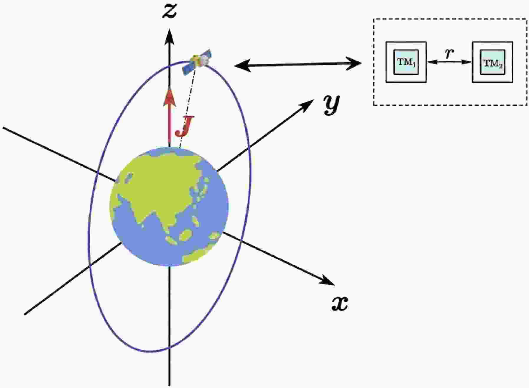
We consider a spacecraft (S/C) in a near-circular polar orbit around the Earth, with orbital radius a and angular frequency ω. The S/C carries two free-falling test masses (TMs), separated by a distance $ d \sim 50{\rm{cm}} $ along the orbital (along-track) direction, forming a one-dimensional gravity gradiometer. We adopt the Earth-centered inertial (ECI) frame as the global reference frame, with coordinates $ (t, x, y, z) $. For simplicity, we assume that the orbit lies in the x-z plane with inclination $ i = 90^\circ $ (polar orbit). The configuration is illustrated in Figs. 1 and 2.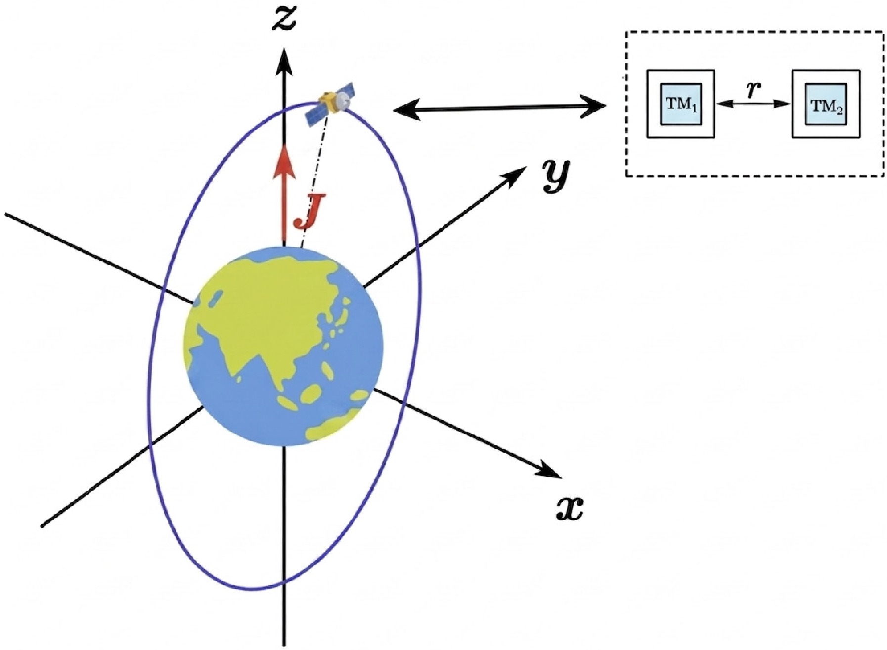

Figure 1.  (color online) Schematic diagram of the polar orbit ($ i = 90^\circ $) used in this work. The orbital plane lies in the x-z plane, and the y axis is perpendicular to it.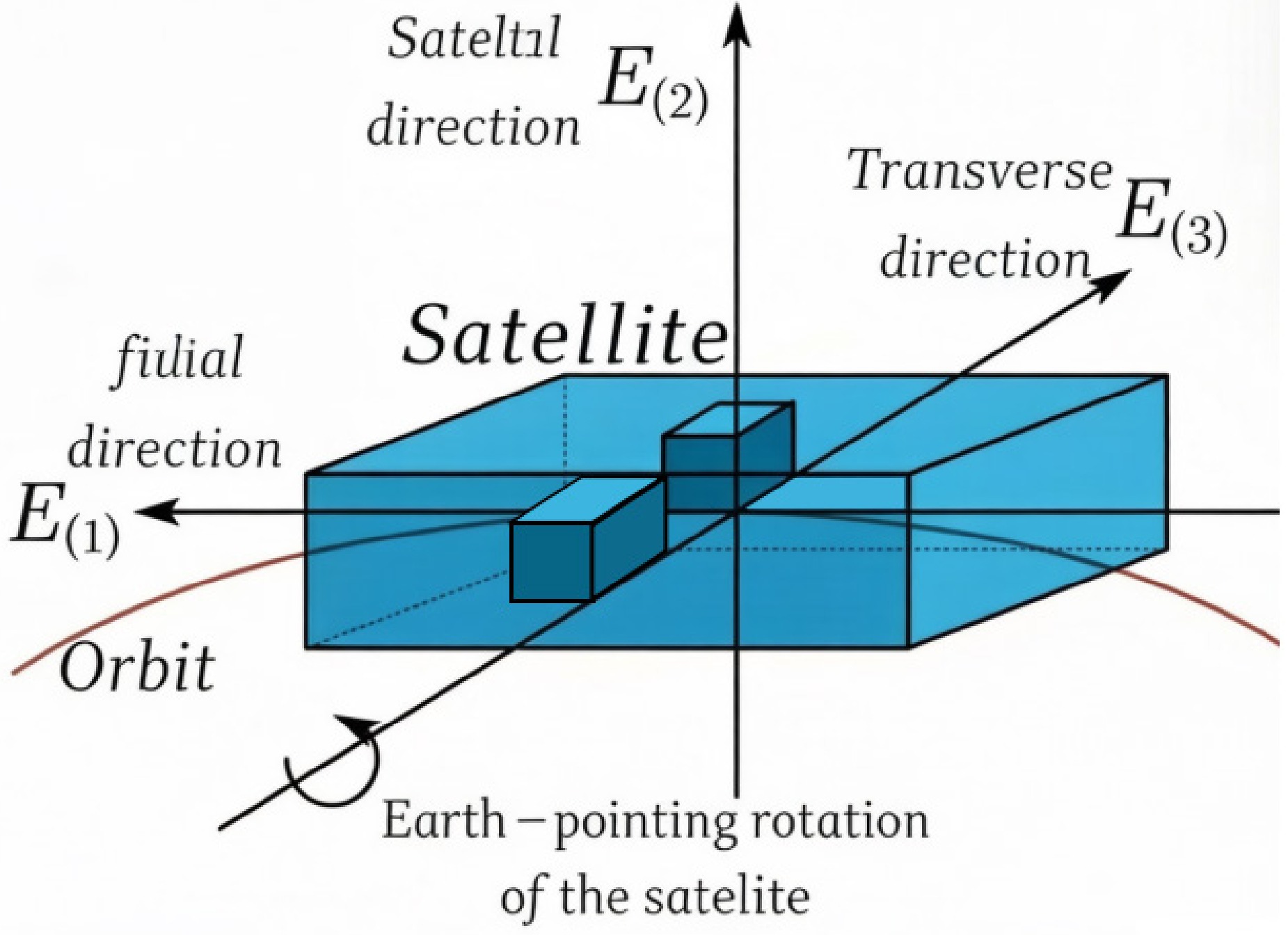

Figure 2.  (color online) Schematic diagram of the spacecraft's polar orbit and gradiometer configuration. Two test masses (TMs) are separated by a distance d in the along-track direction. The local coordinate system is attached to the spacecraft.

The trajectory of the S/C in the ECI frame, including the leading-order gravitomagnetic correction, is given by [18]

where τ denotes the proper time along the orbit, and the Lense–Thirring precession rate $ \Omega_L $ in $ f(R) $ gravity is modified by the effective gravitational constant

Here, J is the Earth's angular momentum, and $ \eta = G_{{\rm{eff}}}/G $, where $ G_{{\rm{eff}}} $ is defined in Eq. (30).

To describe the relative motion of the TMs, we construct a local orthonormal tetrad $ E_{(a)}^\mu $ attached to the S/C, which is Fermi–Walker transported along the orbit. Following the approach in Ref. [15], the tetrad to first post-Newtonian (1PN) order can be expressed as

where M denotes the Earth's mass. This tetrad satisfies $ g_{\mu\nu}E_{(a)}^\mu E_{(b)}^\nu = \eta_{(a)(b)} $ to the required order.

The relative motion of two nearby freely falling test masses is governed by the geodesic deviation equation [12]

where $ X^\mu $ is the separation vector between the two TMs. $ U^\mu $ denotes the four-velocity of the reference worldline (the S/C), and $ R^\mu_{\ \nu\rho\sigma} $ is the Riemann curvature tensor.

In the local tetrad frame, the components of the separation vector are defined as $ X^{(a)} = E^{(a)}_\mu X^\mu $. The geodesic deviation equation in this frame becomes [12]

where $ \gamma^{(a)}_{\ (b)(c)} = E^{(a)}_{\mu} (\nabla_\nu E_{(b)}^\mu) E_{(c)}^\nu $ are the Ricci rotation coefficients, and the tidal matrix $ K^{(a)}_{\ (b)} $ is defined as:

The first two terms in Eq. (40) represent the Coriolis and inertial forces arising from the rotation of the local frame, whereas the last term gives the genuine tidal forces due to spacetime curvature.

To compute the tidal matrix in $ f(R) $ gravity, we need the Riemann tensor components for the metric derived in Section II. In the weak-field limit of Eq. (5), the Riemann tensor to linear order in $ h_{\mu\nu} $ is

Substituting the metric components and evaluating them at the orbital position, we obtain the non-zero components of the tidal matrix in the local tetrad frame. For a polar orbit ($ i = 90^\circ $), the dominant gravitomagnetic contributions to the transverse ($ X^{(3)} $) component arise from:

where $ \epsilon = GM/(ac^2) \sim 10^{-9} $ for a low-Earth orbit.

Substituting the tidal matrix components and rotation coefficients into Eq. (40), and assuming that the TMs are initially aligned in the along-track direction ($ X^{(1)}_0 = -d $, $ X^{(2)}_0 = X^{(3)}_0 = 0 $) with zero relative velocity, we obtain the equation of motion for the transverse displacement $ X^{(3)} $

where dots denote derivatives with respect to τ, and $ \lambda \sim 10^{-3} $ represents small initial misalignment errors. Equation (44) describes a forced harmonic oscillator whose resonant frequency ω equals the driving frequency. The particular solution, representing the steady-state response to the gravitomagnetic driving force, is:

The gravitomagnetic field induces a transverse oscillation of the two test masses, with an amplitude that scales with η and the Earth’s angular momentum $ {\bf{J}} $. This signal increases linearly with the baseline d and decreases with the cube of the orbital radius a. For completeness, we also provide the along-track ($ X^{(1)} $) and cross-track ($ X^{(2)} $) displacements induced by the gravitomagnetic field:

However, these components are either suppressed by a factor of $ \omega\tau $ (which increases with time) or have different frequency content, making them less suitable for precision measurements than the transverse signal.

We consider a spacecraft (S/C) in a near-circular polar orbit around the Earth, with orbital radius a and angular frequency ω. The S/C carries two free-falling test masses (TMs), separated by a distance $ d \sim 50{\rm{cm}} $ along the orbital (along-track) direction, forming a one-dimensional gravity gradiometer. We adopt the Earth-centered inertial (ECI) frame as the global reference frame, with coordinates $ (t, x, y, z) $. For simplicity, we assume that the orbit lies in the x-z plane with inclination $ i = 90^\circ $ (polar orbit). The configuration is illustrated in Figs. 1 and 2.

Figure 1.  (color online) Schematic diagram of the polar orbit ($ i = 90^\circ $) used in this work. The orbital plane lies in the x-z plane, and the y axis is perpendicular to it.

Figure 2.  (color online) Schematic diagram of the spacecraft's polar orbit and gradiometer configuration. Two test masses (TMs) are separated by a distance d in the along-track direction. The local coordinate system is attached to the spacecraft.

The trajectory of the S/C in the ECI frame, including the leading-order gravitomagnetic correction, is given by [18]

where τ denotes the proper time along the orbit, and the Lense–Thirring precession rate $ \Omega_L $ in $ f(R) $ gravity is modified by the effective gravitational constant

Here, J is the Earth's angular momentum, and $ \eta = G_{{\rm{eff}}}/G $, where $ G_{{\rm{eff}}} $ is defined in Eq. (30).

To describe the relative motion of the TMs, we construct a local orthonormal tetrad $ E_{(a)}^\mu $ attached to the S/C, which is Fermi–Walker transported along the orbit. Following the approach in Ref. [15], the tetrad to first post-Newtonian (1PN) order can be expressed as

where M denotes the Earth's mass. This tetrad satisfies $ g_{\mu\nu}E_{(a)}^\mu E_{(b)}^\nu = \eta_{(a)(b)} $ to the required order.

The relative motion of two nearby freely falling test masses is governed by the geodesic deviation equation [12]

where $ X^\mu $ is the separation vector between the two TMs. $ U^\mu $ denotes the four-velocity of the reference worldline (the S/C), and $ R^\mu_{\ \nu\rho\sigma} $ is the Riemann curvature tensor.

In the local tetrad frame, the components of the separation vector are defined as $ X^{(a)} = E^{(a)}_\mu X^\mu $. The geodesic deviation equation in this frame becomes [12]

where $ \gamma^{(a)}_{\ (b)(c)} = E^{(a)}_{\mu} (\nabla_\nu E_{(b)}^\mu) E_{(c)}^\nu $ are the Ricci rotation coefficients, and the tidal matrix $ K^{(a)}_{\ (b)} $ is defined as:

The first two terms in Eq. (40) represent the Coriolis and inertial forces arising from the rotation of the local frame, whereas the last term gives the genuine tidal forces due to spacetime curvature.

To compute the tidal matrix in $ f(R) $ gravity, we need the Riemann tensor components for the metric derived in Section II. In the weak-field limit of Eq. (5), the Riemann tensor to linear order in $ h_{\mu\nu} $ is

Substituting the metric components and evaluating them at the orbital position, we obtain the non-zero components of the tidal matrix in the local tetrad frame. For a polar orbit ($ i = 90^\circ $), the dominant gravitomagnetic contributions to the transverse ($ X^{(3)} $) component arise from:

where $ \epsilon = GM/(ac^2) \sim 10^{-9} $ for a low-Earth orbit.

Substituting the tidal matrix components and rotation coefficients into Eq. (40), and assuming that the TMs are initially aligned in the along-track direction ($ X^{(1)}_0 = -d $, $ X^{(2)}_0 = X^{(3)}_0 = 0 $) with zero relative velocity, we obtain the equation of motion for the transverse displacement $ X^{(3)} $

where dots denote derivatives with respect to τ, and $ \lambda \sim 10^{-3} $ represents small initial misalignment errors. Equation (44) describes a forced harmonic oscillator whose resonant frequency ω equals the driving frequency. The particular solution, representing the steady-state response to the gravitomagnetic driving force, is:

The gravitomagnetic field induces a transverse oscillation of the two test masses, with an amplitude that scales with η and the Earth’s angular momentum $ {\bf{J}} $. This signal increases linearly with the baseline d and decreases with the cube of the orbital radius a. For completeness, we also provide the along-track ($ X^{(1)} $) and cross-track ($ X^{(2)} $) displacements induced by the gravitomagnetic field:

However, these components are either suppressed by a factor of $ \omega\tau $ (which increases with time) or have different frequency content, making them less suitable for precision measurements than the transverse signal.

The precise measurement of gravitational gradients in space relies on advanced technologies capable of detecting extremely weak tidal forces. Two primary instrument types offer exceptional promise for this purpose: superconducting gravity gradiometers (SGGs) and laser interferometric gravity gradiometers (LIGGs). Each technology offers distinct advantages in sensitivity, stability, and operational characteristics for space-based applications.

The superconducting gradiometer concept follows the design pioneered by Paik et al. [17, 22]. The superconducting gravity gradiometer utilizes fundamental properties of superconductors to achieve unprecedented measurement sensitivity. Its operation is based on a superconducting accelerometer that exploits the magnetic interaction between a persistent current-carrying coil and a superconducting test mass in a fully diamagnetic Meissner state. This configuration forms a magnetic spring oscillator that relies on three essential superconducting phenomena. These include the Meissner effect, which enables precise magnetic levitation and position sensing; the zero-resistance effect, which permits persistent currents to circulate without power dissipation; and the Josephson macroscopic quantum effect, which provides ultra-sensitive magnetic flux detection through superconducting quantum interference devices (SQUIDs). A typical SGG configuration employs two or more superconducting accelerometers arranged along each measurement axis, with approximately $ 50cm $ separation between test masses. Differential acceleration sensing is achieved via a superconducting circuit in which gravitational forces induce relative displacements between the test masses and thereby modulate the inductance of the mass-coil systems. In accordance with flux quantization principles, the sensing currents adjust to maintain constant magnetic flux and thereby generate detectable current signals through SQUIDs. Such SGG technology offers several key advantages, including exceptionally low internal noise levels typically below $ 10^{-15} m/s^2/\rm\sqrt{Hz} $ at 0.1mHz; high common-mode rejection, which effectively suppresses disturbances from satellite drag and thermal fluctuations; and cryogenic operation at liquid helium temperatures (4.2K or lower), which minimizes thermal noise while providing excellent environmental stability.

The superconducting gravity gradiometer (SGG) operates on the principle of differential magnetic sensing, enabling the measurement of gravity-gradient variations in three-dimensional space using paired superconducting accelerometers in a differential configuration. The instrument incorporates two superconducting test masses (TMs A and B) magnetically levitated within a cryogenic chamber, with each mass experiencing local gravitational fields $ g_{A} $ and $ g_B $. A persistent-current loop inductively couples the two TMs through superconducting coils. Any relative displacement induced by gravity gradients modulates the mutual inductance of the coil–mass system. This change in inductance alters the persistent current, which is read out by a superconducting quantum interference device (SQUID) to determine the differential acceleration $ \Delta g=g_{B}-g_{A} $. The technology offers several distinct advantages: exceptional sensitivity due to near-zero resistance and quantum-limited detection, high common-mode rejection of platform vibrations and thermal drifts, cryogenic operation at liquid-helium temperatures (typically 4.2 K) for ultra-low intrinsic noise, and a compact design that facilitates integration into space-borne payloads [22]. The relevant design schematics are shown in Figs. 3 and 4.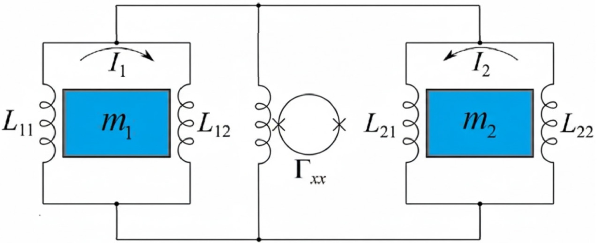

Figure 3.  (color online) Schematic diagram of a superconducting differential acceleration sensing circuit. Two superconducting test masses (TMs) are coupled via persistent-current loops to a SQUID detector, enabling differential measurement of gravitational gradients while rejecting common-mode disturbances.

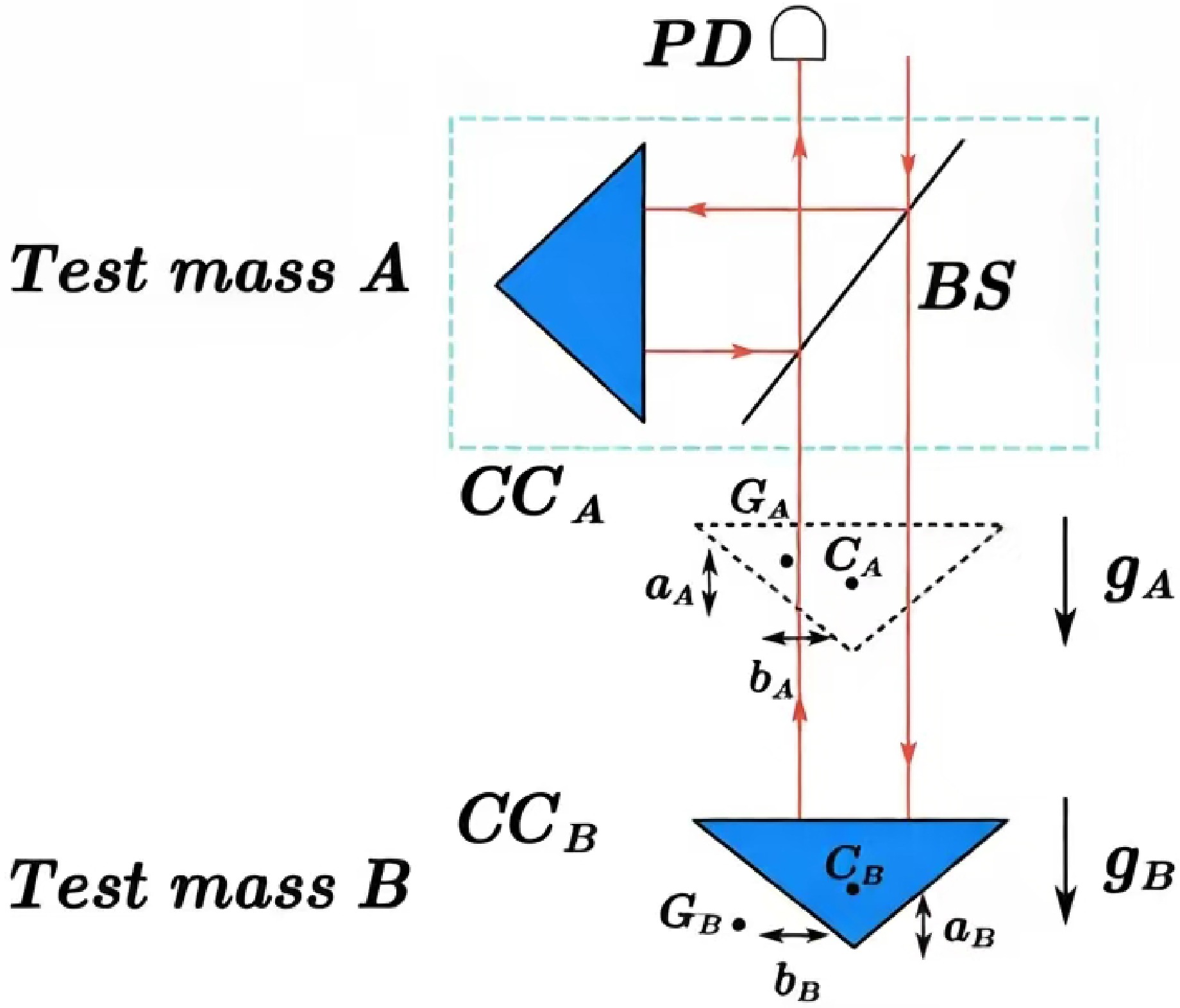
Figure 4.  (color online) Optical layout of a laser interferometric gravity gradiometer. Two test masses (A and B), each containing a corner-cube prism, fall simultaneously in a vacuum chamber. A laser interferometer measures their relative acceleration from interference fringes detected by a photodetector.

The precise measurement of gravitational gradients in space relies on advanced technologies capable of detecting extremely weak tidal forces. Two primary instrument types offer exceptional promise for this purpose: superconducting gravity gradiometers (SGGs) and laser interferometric gravity gradiometers (LIGGs). Each technology offers distinct advantages in sensitivity, stability, and operational characteristics for space-based applications.

The superconducting gradiometer concept follows the design pioneered by Paik et al. [17, 22]. The superconducting gravity gradiometer utilizes fundamental properties of superconductors to achieve unprecedented measurement sensitivity. Its operation is based on a superconducting accelerometer that exploits the magnetic interaction between a persistent current-carrying coil and a superconducting test mass in a fully diamagnetic Meissner state. This configuration forms a magnetic spring oscillator that relies on three essential superconducting phenomena. These include the Meissner effect, which enables precise magnetic levitation and position sensing; the zero-resistance effect, which permits persistent currents to circulate without power dissipation; and the Josephson macroscopic quantum effect, which provides ultra-sensitive magnetic flux detection through superconducting quantum interference devices (SQUIDs). A typical SGG configuration employs two or more superconducting accelerometers arranged along each measurement axis, with approximately $ 50cm $ separation between test masses. Differential acceleration sensing is achieved via a superconducting circuit in which gravitational forces induce relative displacements between the test masses and thereby modulate the inductance of the mass-coil systems. In accordance with flux quantization principles, the sensing currents adjust to maintain constant magnetic flux and thereby generate detectable current signals through SQUIDs. Such SGG technology offers several key advantages, including exceptionally low internal noise levels typically below $ 10^{-15} m/s^2/\rm\sqrt{Hz} $ at 0.1mHz; high common-mode rejection, which effectively suppresses disturbances from satellite drag and thermal fluctuations; and cryogenic operation at liquid helium temperatures (4.2K or lower), which minimizes thermal noise while providing excellent environmental stability.

The superconducting gravity gradiometer (SGG) operates on the principle of differential magnetic sensing, enabling the measurement of gravity-gradient variations in three-dimensional space using paired superconducting accelerometers in a differential configuration. The instrument incorporates two superconducting test masses (TMs A and B) magnetically levitated within a cryogenic chamber, with each mass experiencing local gravitational fields $ g_{A} $ and $ g_B $. A persistent-current loop inductively couples the two TMs through superconducting coils. Any relative displacement induced by gravity gradients modulates the mutual inductance of the coil–mass system. This change in inductance alters the persistent current, which is read out by a superconducting quantum interference device (SQUID) to determine the differential acceleration $ \Delta g=g_{B}-g_{A} $. The technology offers several distinct advantages: exceptional sensitivity due to near-zero resistance and quantum-limited detection, high common-mode rejection of platform vibrations and thermal drifts, cryogenic operation at liquid-helium temperatures (typically 4.2 K) for ultra-low intrinsic noise, and a compact design that facilitates integration into space-borne payloads [22]. The relevant design schematics are shown in Figs. 3 and 4.

Figure 3.  (color online) Schematic diagram of a superconducting differential acceleration sensing circuit. Two superconducting test masses (TMs) are coupled via persistent-current loops to a SQUID detector, enabling differential measurement of gravitational gradients while rejecting common-mode disturbances.

Figure 4.  (color online) Optical layout of a laser interferometric gravity gradiometer. Two test masses (A and B), each containing a corner-cube prism, fall simultaneously in a vacuum chamber. A laser interferometer measures their relative acceleration from interference fringes detected by a photodetector.

Building on the experimental setup described earlier, we constrain the parameters through specific measurements using a single-satellite mission in Earth orbit. The mission parameters include an orbital altitude of 1500 km, a Sun-synchronous circular orbit, an orbital radius of $ a=7.87\times 10^6\,$m, an orbital angular frequency of $\omega= 9.0\times10^{-4}\; \rm rad/s$, an orbital period of 105.5 minutes, a test-mass separation of $ d=0.5\,$m, a mission duration of one year, an inclination of $ i=90 $, and a nadir-pointing satellite attitude. The satellite platform is designed for ultra-stable and ultra-quiet operation, incorporating drag-free control along the critical axes. The payload consists of a dual-axis high-precision laser interferometer for gravitational gradient measurement, a high-precision star-to-ground time-frequency comparison system, and an advanced inertial reference system for attitude determination. Using data from the gradiometer, the satellite achieves two-degree-of-freedom drag-free control along the flight and orbit-normal directions, ensuring optimal operation of the gravitational gradient instrument. The nadir-pointing attitude maintains the instrument's sensitive axis perpendicular to the orbital plane, maximizing sensitivity to the transverse gravitomagnetic signal.

From the theoretical derivation in Section III, the transverse gravitomagnetic signal is given by

where the amplitude is

By substituting numerical values for all the parameters, we obtain

The signal appears at the orbital frequency $ f_{{\rm{orb}}} = \omega / (2\pi) \approx 0.144 \, {\rm{mHz}} $, which lies well within the measurement bandwidth of both SGG and LIGG technologies.

The fundamental sensitivity limit of gravitational gradiometers is set by several noise sources, including instrument noise, seismic noise (negligible in orbit), thermal noise, magnetic noise, and satellite platform noise. For our mission, we assume a baseline sensitivity of $ 10^{-2}\,{\rm{s}}^{-2}/\sqrt{{\rm{Hz}}} $ at $ 0.144 \, {\rm{mHz}} $, consistent with LIGG performance. Over a one-year integration period ($ T = 3.156 \times 10^{7}{\rm{s}} $), the equivalent noise in gradient measurement is

This corresponds to a displacement noise between the two TMs of

The signal-to-noise ratio (SNR) for detecting the gravitomagnetic signal is

For a statistically significant detection ($ {\rm{SNR}} \geq 5 $), we require $ \eta \geq 0.092 $, which is easily satisfied since $ \eta \approx 1 $ in standard gravity. The precision with which η can be determined is given by

However, this represents only the statistical uncertainty. Systematic errors must also be taken into account. Based on detailed error budgets from missions such as LISA Pathfinder and GOCE, we estimate that systematic errors in the gradient measurement contribute an additional uncertainty of approximately 30% of the statistical uncertainty. Therefore, the total uncertainty in η is

Since $ \eta=G_{\rm{eff}}/G $, this imposes a constraint on the deviation of Newton's constant:

This preliminary estimate can be substantially improved through several factors: extending the mission duration to $ 3 $–$ 5 $ years would reduce the statistical noise by a factor of $ \sqrt{3} $ to $ \sqrt{5} $; employing next-generation gradiometers (which target sensitivities of $ 10^{-3}{\rm{s}}^{-2} /\sqrt{{\rm{Hz}}} $); and applying optimal narrow-band filtering around the signal frequency, which would yield an additional noise reduction by a factor of $ 2 $–$ 3 $. Incorporating these enhancements yields a projected constraint of $ |\eta-1| \lesssim 0.0025 $.

which represents an improvement of one to two orders of magnitude over the current experimental bounds set by the GP-B and LAGEOS missions.

For the quadratic model $ f(R)=R+\alpha R^2 $, the parameter η is related to the scalar mass $ m_s $ and the orbital radius a through

In dimensionless form, using the Earth's orbital scale, we obtain:

This represents the most stringent constraint on quadratic $ f(R) $ gravity from gravitomagnetic measurements to date, improving upon previous bounds from solar-system tests. It is worth emphasizing that this bound corresponds to the enhanced mission projection described in Eq. (56), rather than the baseline estimate in Eq. (55).

In contrast to absolute measurements such as satellite laser ranging (LAGEOS) or gyroscope experiments (Gravity Probe B), the differential gradiometer scheme proposed here strongly suppresses common-mode disturbances. Nevertheless, residual systematic effects must be carefully quantified.

A quantitative error budget is summarized in Table 1. The root-sum-square of the identified contributions is approximately 13% of the statistical error. To be conservative and to account for possible unmodeled residuals, we adopt a total systematic uncertainty of 30% of the statistical error in our final constraint on η.

Building on the experimental setup described earlier, we constrain the parameters through specific measurements using a single-satellite mission in Earth orbit. The mission parameters include an orbital altitude of 1500 km, a Sun-synchronous circular orbit, an orbital radius of $ a=7.87\times 10^6\,$m, an orbital angular frequency of $\omega= 9.0\times10^{-4}\; \rm rad/s$, an orbital period of 105.5 minutes, a test-mass separation of $ d=0.5\,$m, a mission duration of one year, an inclination of $ i=90 $, and a nadir-pointing satellite attitude. The satellite platform is designed for ultra-stable and ultra-quiet operation, incorporating drag-free control along the critical axes. The payload consists of a dual-axis high-precision laser interferometer for gravitational gradient measurement, a high-precision star-to-ground time-frequency comparison system, and an advanced inertial reference system for attitude determination. Using data from the gradiometer, the satellite achieves two-degree-of-freedom drag-free control along the flight and orbit-normal directions, ensuring optimal operation of the gravitational gradient instrument. The nadir-pointing attitude maintains the instrument's sensitive axis perpendicular to the orbital plane, maximizing sensitivity to the transverse gravitomagnetic signal.

From the theoretical derivation in Section III, the transverse gravitomagnetic signal is given by

where the amplitude is

By substituting numerical values for all the parameters, we obtain

The signal appears at the orbital frequency $ f_{{\rm{orb}}} = \omega / (2\pi) \approx 0.144 \, {\rm{mHz}} $, which lies well within the measurement bandwidth of both SGG and LIGG technologies.

The fundamental sensitivity limit of gravitational gradiometers is set by several noise sources, including instrument noise, seismic noise (negligible in orbit), thermal noise, magnetic noise, and satellite platform noise. For our mission, we assume a baseline sensitivity of $ 10^{-2}\,{\rm{s}}^{-2}/\sqrt{{\rm{Hz}}} $ at $ 0.144 \, {\rm{mHz}} $, consistent with LIGG performance. Over a one-year integration period ($ T = 3.156 \times 10^{7}{\rm{s}} $), the equivalent noise in gradient measurement is

This corresponds to a displacement noise between the two TMs of

The signal-to-noise ratio (SNR) for detecting the gravitomagnetic signal is

For a statistically significant detection ($ {\rm{SNR}} \geq 5 $), we require $ \eta \geq 0.092 $, which is easily satisfied since $ \eta \approx 1 $ in standard gravity. The precision with which η can be determined is given by

However, this represents only the statistical uncertainty. Systematic errors must also be taken into account. Based on detailed error budgets from missions such as LISA Pathfinder and GOCE, we estimate that systematic errors in the gradient measurement contribute an additional uncertainty of approximately 30% of the statistical uncertainty. Therefore, the total uncertainty in η is

Since $ \eta=G_{\rm{eff}}/G $, this imposes a constraint on the deviation of Newton's constant:

This preliminary estimate can be substantially improved through several factors: extending the mission duration to $ 3 $–$ 5 $ years would reduce the statistical noise by a factor of $ \sqrt{3} $ to $ \sqrt{5} $; employing next-generation gradiometers (which target sensitivities of $ 10^{-3}{\rm{s}}^{-2} /\sqrt{{\rm{Hz}}} $); and applying optimal narrow-band filtering around the signal frequency, which would yield an additional noise reduction by a factor of $ 2 $–$ 3 $. Incorporating these enhancements yields a projected constraint of $ |\eta-1| \lesssim 0.0025 $.

which represents an improvement of one to two orders of magnitude over the current experimental bounds set by the GP-B and LAGEOS missions.

For the quadratic model $ f(R)=R+\alpha R^2 $, the parameter η is related to the scalar mass $ m_s $ and the orbital radius a through

In dimensionless form, using the Earth's orbital scale, we obtain:

This represents the most stringent constraint on quadratic $ f(R) $ gravity from gravitomagnetic measurements to date, improving upon previous bounds from solar-system tests. It is worth emphasizing that this bound corresponds to the enhanced mission projection described in Eq. (56), rather than the baseline estimate in Eq. (55).

In contrast to absolute measurements such as satellite laser ranging (LAGEOS) or gyroscope experiments (Gravity Probe B), the differential gradiometer scheme proposed here strongly suppresses common-mode disturbances. Nevertheless, residual systematic effects must be carefully quantified.

A quantitative error budget is summarized in Table 1. The root-sum-square of the identified contributions is approximately 13% of the statistical error. To be conservative and to account for possible unmodeled residuals, we adopt a total systematic uncertainty of 30% of the statistical error in our final constraint on η.

In this paper, we develop a comprehensive framework for testing $ f(R) $ modified gravity through high-precision, space-based measurements of the planetary gravitomagnetic field. By analyzing the Lense–Thirring effect within the parametrized post-Newtonian formalism, we derive the gravitomagnetic tidal signal, which depends on the effective gravitational constant $ G_{{\rm{eff}}} $ in $ f(R) $ gravity. The transverse oscillation induced by frame dragging between two freely falling test masses provides a clean and direct probe of deviations from general relativity.

Our proposed differential measurement scheme, based on a superconducting or laser-interferometric gravity gradiometer in low Earth orbit, offers significant advantages over traditional gravitomagnetic experiments. By eliminating the need for an external global inertial reference frame, this approach reduces systematic errors associated with satellite laser ranging and gyroscope-based measurements. The differential design also improves common-mode rejection of platform vibrations and thermal disturbances, enabling unprecedented sensitivity to gravitational gradients.

For a one-year mission at an altitude of 1500 km with a gradiometer sensitivity of $ 10^{-2}\; \ {{s}}^{-2}/\sqrt{{\rm{Hz}}} $ at the orbital frequency, we project a constraint of $ |\eta - 1| \lesssim 0.0025 $ on the deviation of the effective gravitational constant from its Newtonian value. This corresponds to an upper bound on the quadratic coupling parameter $ \alpha \lesssim 6.9 \times 10^{10}\; {\rm{m}}^2 $ in the $ f(R) = R + \alpha R^2 $ model, improving upon existing gravitomagnetic constraints from Gravity Probe B and LAGEOS by approximately one to two orders of magnitude. These results establish gravitomagnetic measurements as a competitive and complementary approach to Solar System tests of gravity.

The experimental methodology presented here is well aligned with current technological capabilities. Both superconducting and laser-interferometric gradiometers have reached sufficient maturity for space deployment, as demonstrated by pathfinder missions such as LISA Pathfinder and GOCE. Future improvements in instrument sensitivity, mission duration, and data analysis techniques could further tighten these constraints, potentially reaching the $ 10^{-4} $ level in $ |\eta - 1| $ with next-generation sensors and extended operation.

Beyond $ f(R) $ gravity, the framework developed in this work can be extended to other modified gravity theories that predict deviations in the gravitomagnetic sector, including scalar-tensor theories, Hořava–Lifshitz gravity, and non-local modifications. The ability to probe the coupling between gravity and angular momentum at this level of precision opens new avenues for testing fundamental aspects of gravitational theory that are inaccessible to static or radially symmetric measurements.

It is also useful to compare the sensitivity of our proposed gravitomagnetic measurement with that of light-deflection experiments such as Cassini. The latter constrains the PPN parameter γ at a distance of about $ 1\,{\rm{AU}} $. For a light scalar field ($ m_s^{-1} \gg 1\,{\rm{AU}} $), the deviation $ \gamma-1 $ scales as $ m_s^2 r^2 $, leading to a relatively weak bound on the quadratic coupling $ \alpha = 1/(6m_s^2) $. In contrast, our experiment operates at an orbital radius $ a\ll1\,{\rm{AU}} $; for the same $ m_s $, the gravitomagnetic signal $ \eta-1 $ is not exponentially suppressed when $ m_s a\ll1 $ and can be orders of magnitude larger than the corresponding light-deflection signal. Therefore, the two methods are complementary: Cassini is more sensitive to very light scalars (with extremely large α), whereas our scheme is more sensitive to scalars with Compton wavelengths comparable to Earth-orbit distances. Thus, the tighter bound we project is not contradictory, but rather reflects the different distance scales probed.

In summary, this study demonstrates that space-based gravity gradiometry offers a powerful and feasible means of testing modifications of general relativity through gravitomagnetic effects. By providing a direct measurement of frame dragging with significantly reduced systematic uncertainties, the proposed experiment could deliver decisive constraints on alternative gravity theories and contribute to our understanding of gravity at both macroscopic and cosmological scales. As space missions continue to advance in precision and duration, gravitomagnetic measurements are poised to become an increasingly important component of the experimental gravity landscape.

In this paper, we develop a comprehensive framework for testing $ f(R) $ modified gravity through high-precision, space-based measurements of the planetary gravitomagnetic field. By analyzing the Lense–Thirring effect within the parametrized post-Newtonian formalism, we derive the gravitomagnetic tidal signal, which depends on the effective gravitational constant $ G_{{\rm{eff}}} $ in $ f(R) $ gravity. The transverse oscillation induced by frame dragging between two freely falling test masses provides a clean and direct probe of deviations from general relativity.

Our proposed differential measurement scheme, based on a superconducting or laser-interferometric gravity gradiometer in low Earth orbit, offers significant advantages over traditional gravitomagnetic experiments. By eliminating the need for an external global inertial reference frame, this approach reduces systematic errors associated with satellite laser ranging and gyroscope-based measurements. The differential design also improves common-mode rejection of platform vibrations and thermal disturbances, enabling unprecedented sensitivity to gravitational gradients.

For a one-year mission at an altitude of 1500 km with a gradiometer sensitivity of $ 10^{-2}\; \ {{s}}^{-2}/\sqrt{{\rm{Hz}}} $ at the orbital frequency, we project a constraint of $ |\eta - 1| \lesssim 0.0025 $ on the deviation of the effective gravitational constant from its Newtonian value. This corresponds to an upper bound on the quadratic coupling parameter $ \alpha \lesssim 6.9 \times 10^{10}\; {\rm{m}}^2 $ in the $ f(R) = R + \alpha R^2 $ model, improving upon existing gravitomagnetic constraints from Gravity Probe B and LAGEOS by approximately one to two orders of magnitude. These results establish gravitomagnetic measurements as a competitive and complementary approach to Solar System tests of gravity.

The experimental methodology presented here is well aligned with current technological capabilities. Both superconducting and laser-interferometric gradiometers have reached sufficient maturity for space deployment, as demonstrated by pathfinder missions such as LISA Pathfinder and GOCE. Future improvements in instrument sensitivity, mission duration, and data analysis techniques could further tighten these constraints, potentially reaching the $ 10^{-4} $ level in $ |\eta - 1| $ with next-generation sensors and extended operation.

Beyond $ f(R) $ gravity, the framework developed in this work can be extended to other modified gravity theories that predict deviations in the gravitomagnetic sector, including scalar-tensor theories, Hořava–Lifshitz gravity, and non-local modifications. The ability to probe the coupling between gravity and angular momentum at this level of precision opens new avenues for testing fundamental aspects of gravitational theory that are inaccessible to static or radially symmetric measurements.

It is also useful to compare the sensitivity of our proposed gravitomagnetic measurement with that of light-deflection experiments such as Cassini. The latter constrains the PPN parameter γ at a distance of about $ 1\,{\rm{AU}} $. For a light scalar field ($ m_s^{-1} \gg 1\,{\rm{AU}} $), the deviation $ \gamma-1 $ scales as $ m_s^2 r^2 $, leading to a relatively weak bound on the quadratic coupling $ \alpha = 1/(6m_s^2) $. In contrast, our experiment operates at an orbital radius $ a\ll1\,{\rm{AU}} $; for the same $ m_s $, the gravitomagnetic signal $ \eta-1 $ is not exponentially suppressed when $ m_s a\ll1 $ and can be orders of magnitude larger than the corresponding light-deflection signal. Therefore, the two methods are complementary: Cassini is more sensitive to very light scalars (with extremely large α), whereas our scheme is more sensitive to scalars with Compton wavelengths comparable to Earth-orbit distances. Thus, the tighter bound we project is not contradictory, but rather reflects the different distance scales probed.

In summary, this study demonstrates that space-based gravity gradiometry offers a powerful and feasible means of testing modifications of general relativity through gravitomagnetic effects. By providing a direct measurement of frame dragging with significantly reduced systematic uncertainties, the proposed experiment could deliver decisive constraints on alternative gravity theories and contribute to our understanding of gravity at both macroscopic and cosmological scales. As space missions continue to advance in precision and duration, gravitomagnetic measurements are poised to become an increasingly important component of the experimental gravity landscape.