


 Abstract
 HTML
 Reference
 Related
 PDF



-
Black holes in realistic astrophysical environments are not isolated systems; rather, they are embedded in complex structures composed of baryonic matter, plasma, and dark matter. Observational evidence strongly supports the existence of supermassive black holes at the centers of galaxies [1, 2], while galactic systems themselves are known to reside within extended dark matter halos [3]. It is therefore clear that the idealized description of black holes as vacuum solutions must be refined by incorporating the gravitational influence of surrounding matter distributions, especially when addressing dynamical processes that are sensitive to the global spacetime structure.
Among the most significant phenomena in rotating black hole physics are quasibound states (QBSs) and superradiant scattering, both of which arise from the interaction between bosonic fields and curved spacetime. Quasibound states correspond to long-lived oscillatory configurations localized outside the event horizon. They arise when the effective potential develops a confining structure capable of trapping perturbations [4−9]. Their complex frequencies encode both oscillation and decay rates, thereby providing a sensitive probe of the underlying geometry. We note that, in rotating spacetimes, these modes become particularly relevant because they are directly connected to superradiant energy extraction and may signal the onset of instabilities.
Superradiance is a wave-amplification mechanism in which an incident bosonic field scatters off a rotating horizon and emerges with increased amplitude, thereby extracting rotational energy from the black hole when the superradiant condition is satisfied [10]. This process plays a central role in black hole bomb scenarios, ultralight boson phenomenology, and stability analyses of rotating compact objects. The amplification factor provides a direct quantitative measure of this effect and therefore constitutes a key observable in scattering theory.
Because both quasibound spectra and superradiant amplification depend sensitively on the structure of the effective potential, they provide a natural framework for probing environmental effects. In particular, the presence of a surrounding dark matter halo can deform the gravitational potential, modify the trapping structure of scalar perturbations, shift resonant frequencies, and alter the efficiency of superradiant scattering. Understanding these modifications is therefore essential for establishing how realistic astrophysical environments influence the dynamical response of rotating black holes.
Motivated by these considerations, considerable attention has been devoted to constructing black hole solutions embedded in dark matter halos with the aim of capturing realistic astrophysical environments. Different halo profiles induce distinct modifications of the spacetime geometry and its associated observables. For instance, black hole shadows, geodesic motion, and wave propagation have been analyzed in Hernquist-type geometries [11, 12], while alternative constructions include universal rotation curve models, piecewise halo metrics, and rotating configurations immersed in cold or scalar-field dark matter backgrounds [13−15]. Additional studies have explored optical properties, thermodynamics, gravitational lensing, and photon dynamics in such systems [16−23], making it clear that environmental effects can leave observable imprints across a wide range of phenomena.
In this context, particular emphasis has recently been placed on black hole configurations embedded in Dehnen-type double power-law dark matter distributions, which provide a flexible and physically well-motivated framework for modeling galactic halos. A variety of specific realizations within the
$ (1,4,\gamma) $ family have been investigated, including$ (1,4,0) $ [24],$ \left(1,4,\dfrac{1}{2}\right) $ [25],$ (1,4,1) $ [26],$ \left(1,4,\dfrac{3}{2}\right) $ [27],$ (1,4,2) $ [28], and$ \left(1,4,\dfrac{5}{2}\right) $ [29, 30]. It is clear that the Dehnen class is particularly powerful because the inner slope parameter γ allows one to interpolate continuously between cored and cuspy halo structures while preserving a universal outer behavior. Such profiles can significantly influence black hole physics by modifying thermodynamic quantities, altering gravitational lensing signatures, and reshaping the structure of black hole shadows [31]. This versatility makes the Dehnen$ (1,4,\gamma) $ family an ideal setting for systematically exploring how dark matter environments affect both the geometric and dynamical properties of black holes.A particularly general and physically motivated class of models is provided by the double power-law family of density profiles [32, 33], defined by
$ \rho(r)=\rho_0\left(\dfrac{r}{r_0}\right)^{-\gamma} \left[1+\left(\dfrac{r}{r_0}\right)^\alpha \right]^{\tfrac{\gamma-\beta}{\alpha}}. $
(1) Here, the parameters
$ (\alpha,\beta,\gamma) $ control the transition behavior, outer slope, and inner slope, respectively. This parametrization unifies a broad class of halo models, including the Navarro–Frenk–White, Hernquist, Plummer, Burkert, and pseudo-isothermal profiles [27, 34−36], thereby enabling a systematic exploration of both cuspy and cored dark matter distributions within a single analytic framework.In the present work, we focus on the Dehnen family, characterized by
$ (\alpha,\beta,\gamma)=(1,4,\gamma), $ for which the density profile reduces to$ \rho_{\rm{DM}}(r)=\rho_0 \left(\dfrac{r}{r_0}\right)^{-\gamma} \left(1+\dfrac{r}{r_0}\right)^{\gamma-4}. $
(2) We note that this model smoothly interpolates between different inner density behaviors controlled by γ, while preserving the universal outer falloff
$ \rho\sim r^{-4} $ . These results show that varying γ provides a controlled means of probing how the inner structure of the halo influences black hole dynamics, making the Dehnen$ (1,4,\gamma) $ profile particularly suitable for our analysis.Recently, black hole spacetimes surrounded by dark matter halos have been proposed in various scenarios. However, not all such constructions are derived as exact solutions of the Einstein field equations, which may lead to inconsistencies between the metric and the underlying matter distribution [?]. In this work, we address this issue by constructing a self-consistent Schwarzschild–Dehnen solution directly from the Einstein equations, thereby ensuring that the prescribed dark matter density profile is faithfully reproduced.
Building on this exact static configuration, we generate its rotating counterpart via the Newman–Janis algorithm and investigate the dynamics of massive scalar perturbations in the resulting spacetime. Our primary objective is to determine how the Dehnen
$ (1,4,\gamma) $ dark matter halo modifies the quasibound-state spectrum and the superradiant scattering properties of the rotating black hole.To this end, we employ the analytical asymptotic matching (AAM) method [37−40]. In the near-horizon region, the radial equation reduces to a hypergeometric form, with solutions expressed in terms of
$ {}_2F_1 $ functions that satisfy purely ingoing boundary conditions. In the far-field region, the equation simplifies to a confluent hypergeometric form, whose solutions are expressed in terms of$ {}_1F_1 $ functions. By matching these solutions in the overlap region, we obtain analytic expressions for both the quasibound-state spectrum and the superradiant amplification factor.In this work, we show that the presence of the Dehnen halo modifies the effective potential, leading to measurable shifts in the resonance spectrum of quasibound states and altering the efficiency of superradiant amplification. In this sense, the results demonstrate that quasibound modes and superradiant scattering are complementary aspects of a unified spectral structure, encoding how rotating black holes respond to their dark matter environment.
The remainder of this paper is organized as follows. In Sec. II, we construct the exact static Schwarzschild–Dehnen solution. In Sec. III, we generate the rotating geometry via the Newman–Janis algorithm. In Sec. IV, we analyze scalar perturbations, derive the radial equation, and study quasibound states and superradiant amplification. Finally, in Sec. V, we summarize our findings and conclude.
-
To construct a self-consistent black hole solution embedded in a Dehnen dark matter environment, we consider a static, spherically symmetric spacetime sourced by a central compact object surrounded by a
$ (1,4,\gamma) $ halo distribution. The most general metric ansatz consistent with these symmetries can be written as$ {\rm d} s^2=-f(r){\rm d}t^2+\dfrac{{\rm d}r^2}{f(r)}+r^2\left({\rm d}\theta^2+\sin^2\theta\,{\rm d}\phi^2\right), $
(3) where the metric function
$ f(r) $ encodes the combined gravitational effects of the black hole and the surrounding dark matter halo.To model the halo contribution, we assume that the matter source is described by an anisotropic-fluid energy– momentum tensor of the form
$ T^\mu_{\ \nu} = \text{diag} \left[ -\rho_{\rm{DM}}(r),\,p_r(r),\,p_t(r),\,p_t(r) \right], $
(4) where
$ \rho_{\rm{DM}}(r) $ denotes the dark matter energy density, while$ p_r(r) $ and$ p_t(r) $ denote the radial and tangential pressures, respectively. Such anisotropic configurations arise naturally in extended halo models, in which the internal stresses need not be isotropic.Substituting the metric ansatz (3) into Einstein's field equations yields the nonvanishing components
● Temporal component
$ G_{tt} = -\dfrac{f(r)}{r^2} \left[ r f'(r)+f(r)-1 \right] = 8\pi f(r)\rho_{\rm{DM}}(r), $
(5) ● Radial component
$ G_{rr} = \dfrac{1}{r^2f(r)} \left[ r f'(r)+f(r)-1 \right] = 8\pi \dfrac{p_r(r)}{f(r)}, $
(6) ● Angular components
$ G_{\theta\theta} = \dfrac{G_{\phi\phi}}{\sin^2\theta} = {\dfrac{r^2}{2}f''(r)+rf'(r) }= 8\pi r^2p_t(r). $
(7) Here, primes denote differentiation with respect to the radial coordinate. The first two equations imply the following relation.
$ p_r(r)=-\rho_{\rm{DM}}(r), $
(8) which indicates that the radial pressure is equal in magnitude to, and opposite in sign from, the energy density.
The temporal field equation can be rewritten in compact form
$ \dfrac{{\rm d}}{{\rm d}r}\bigl[r(1-f(r))\bigr]=-8\pi r^2\rho_{\rm{DM}}(r), $
(9) which directly determines the metric once the density profile has been specified. By integrating and imposing the correct Schwarzschild limit, we obtain
$ f(r) = 1-\dfrac{r_s}{r} -\dfrac{8\pi}{r} \int_0^r \rho_{\rm{DM}}(r')\,r'^2\,{\rm d}r', $
(10) where
$ r_s=2M $ is the Schwarzschild radius. This expression clearly separates the vacuum contribution from the cumulative mass contribution of the dark matter halo.For the Dehnen
$ (1,4,\gamma) $ profile, the density is given by$ \rho_{\rm{DM}}(r) = \rho_0 \left(\dfrac{r}{r_0}\right)^{-\gamma} \left(1 + \dfrac{r}{r_0}\right)^{\gamma - 4}, $
(11) where
$ \rho_0 $ and$ r_0 $ denote the characteristic density and the scale radius, respectively.Substituting this profile into the integral expression and performing the integration analytically, we obtain
$ f(r) = 1 - \dfrac{r_s}{r} - \dfrac{8\pi \rho_0 r_0^3}{3-\gamma}\, r^{2 - \gamma} (r + r_0)^{3-\gamma}, $
(12) where
$ r_s = 2M $ and$ 0 \leqslant \gamma \lt 3 $ .In the vacuum limit,
$ \rho_0 = 0 $ , the dark matter contribution vanishes, and the metric reduces to the standard Schwarzschild solution, as expected. -
Astrophysical black holes are expected to possess angular momentum, making rotation an essential ingredient in any realistic spacetime description. To extend the static Schwarzschild–Dehnen solution to a rotating geometry, we employ the Newman–Janis algorithm (NJA) [41, 42]. While the original NJA was introduced through a complex coordinate transformation that generates the Kerr metric from the Schwarzschild solution [43], we adopt the modern formulation developed by Azreg-Aïnou [44], which eliminates the ambiguities associated with the complexification procedure and has become a standard tool for constructing rotating counterparts of static black-hole spacetimes. It was shown in [44] that this prescription yields rotating solutions consistent with the Einstein field equations for a broad class of nonvacuum spacetimes with nonvanishing energy density and pressure. This prescription has also been widely employed in the literature, including for nonvacuum and matter-supported geometries, and has proven remarkably successful in studies of black-hole thermodynamics, shadows, quasinormal modes, superradiance, and gravitational lensing [45−55].
We start from the general static, spherically symmetric line element
$ {\rm d}s^2=-F(r)\,{\rm d}t^2+\dfrac{{\rm d}r^2}{G(r)}+H(r)\left({\rm d}\theta^2+\sin^2\theta\,{\rm d}\phi^2\right), $
(13) which, in the Schwarzschild–Dehnen configuration, reduces to
$ F(r)=G(r)=f(r), \qquad H(r)=r^2. $
(14) As a first step, the metric is rewritten in advanced Eddington–Finkelstein coordinates as follows:
$ {\rm d}t={\rm d}u+\dfrac{{\rm d}r}{\sqrt{F(r)G(r)}}. $
(15) This choice removes coordinate singularities at the horizon and allows a regular null formulation of the geometry.
The inverse metric can then be expressed in terms of the Newman–Penrose null tetrad basis
$ g^{\mu\nu} = -l^{\mu}n^{\nu} -l^{\nu}n^{\mu} +m^{\mu}\bar m^{\nu} +m^{\nu}\bar m^{\mu}, $
(16) with tetrads chosen as
$ \begin{aligned}[b] &l^{\mu} =\delta_r^\mu,\\ &n^{\mu} =\delta_u^\mu-\dfrac12F(r)\delta_r^\mu,\\ &m^{\mu} =\dfrac{1}{\sqrt{2H(r)}}\left(\delta_\theta^\mu+\dfrac{\rm i}{\sin\theta}\delta_\phi^\mu\right). \end{aligned} $
(17) Here,
$ \bar m^\mu $ denotes the complex conjugate. These vectors satisfy the standard null normalization and orthogonality conditions.Rotation is then introduced through the complex transformation
$ u\rightarrow u-{\rm i}a\;\cos\;\theta,\qquad r\rightarrow r+{\rm i}a\;\cos\;\theta, $
(18) where a denotes the specific angular momentum of the black hole. This step effectively couples the radial and angular sectors of the geometry, thereby generating frame-dragging effects.
To ensure a consistent extension, we follow the refined prescription of Refs. [44, 56] and promote the metric functions according to
$ F(r),\,G(r),\,H(r)\;\longrightarrow\;A(r,\theta),\,B(r,\theta),\,\rho^2, $
(19) with
$ \rho^2=r^2+a^2\cos^2\theta. $
(20) After reconstructing the metric from the transformed tetrads, the line element in Eddington–Finkelstein coordinates is given by
$ \begin{aligned}[b] {\rm d}s^2 =& -{\cal{F}}\,{\rm d}u^2 -2\,{\rm d}u\,{\rm d}r +2({\cal{F}}-1)a\sin^2\theta\,{\rm d}u\,{\rm d}\phi \\ &+ 2a\sin^2\theta\,{\rm d}r\,{\rm d}\phi + \rho^2\,{\rm d}\theta^2 \\ & +\sin^2\theta \left[ \rho^2 + (2 -{\cal{F}})a^2\sin^2\theta \right] {\rm d}\phi^2, \end{aligned}$
(21) where
$ {\cal{F}}(r,\theta) $ represents the deformation induced by rotation.To express the metric in Boyer–Lindquist form, we perform the coordinate transformation
$ {\rm d}u={\rm d}t-\dfrac{r^2+a^2}{\Delta}\,{\rm d}r,\qquad {\rm d}\phi={\rm d}\varphi-\dfrac{a}{\Delta}\,{\rm d}r, $
(22) and impose the conditions
$ g_{tr}=g_{r\varphi}=0 $ , which eliminate the mixed radial terms. This requirement uniquely determines the lapse function as$ {\cal{F}}=\dfrac{\Delta-a^2\sin^2\theta}{\rho^2}. $
(23) The remaining metric functions are determined by enforcing the appropriate limiting behaviors. In particular, the solution must reduce to the static Schwarzschild–Dehnen geometry as
$ a\to0 $ and to the Kerr spacetime in the absence of dark matter. This yields$ \Delta(r)=r^2 f(r)+a^2, \qquad {\cal{F}}(r,\theta)=1-\dfrac{r^2\bigl(1-f(r)\bigr)}{\rho^2}. $
(24) It is worth noting that the Dehnen halo modifies
$ \Delta(r) $ through the function$ f(r) $ , thereby altering the horizon structure and the ergoregion. In particular, increasing the inner slope parameter γ enhances the central concentration of dark matter, which in turn leads to stronger deviations from the Kerr geometry near the horizon.Combining these elements, the rotating Schwarzschild–Dehnen solution can be written as
$\begin{aligned}[b] {\rm d}s^2=&-\left(1-\dfrac{\xi(r)}{\rho^2}\right){\rm d}t^2+\dfrac{\rho^2}{\Delta}{\rm d}r^2+\rho^2 {\rm d}\theta^2\\ & - 2\dfrac{\xi(r)}{\rho^2}a\sin^2\theta\,{\rm d}t\,{\rm d}\varphi + \dfrac{\Sigma(r,\theta)}{\rho^2}\sin^2\theta\,{\rm d}\varphi^2, \end{aligned} $
(25) where
$ \qquad\qquad\xi(r)=r^2\bigl(1-f(r)\bigr), $
(26) $\qquad\qquad \Delta(r)=r^2+a^2-\xi(r), $
(27) $\qquad\qquad \Sigma(r,\theta)=(r^2+a^2)^2-\Delta a^2\sin^2\theta. $
(28) This metric represents the rotating counterpart of the Schwarzschild–Dehnen black hole and serves as the background for analyzing scalar perturbations, quasibound states, and superradiant scattering. In the limit
$ \rho_0\to0 $ , one recovers$ f(r)=1-2M/r $ , yielding$ \Delta=r^2-2Mr+a^2, $
(29) so that the spacetime reduces exactly to the Kerr solution, as expected.
-
We now turn to the propagation of scalar fields in the rotating Schwarzschild–Dehnen background to uncover the resonant structure of the spacetime. The analysis begins with the inverse metric, which encodes the dynamical couplings among the temporal, radial, and angular sectors. Writing the covariant metric in matrix form
$\begin{aligned}[b] &g_{\mu \nu }=\\ &\left( \begin{array}{cccc} -\dfrac{\Delta -a^2\sin^{2}\theta}{\rho^2} & 0 & 0 & -\dfrac{a\sin^2\theta\,(r^2+a^2-\Delta)}{\rho^2} \\ 0 & \dfrac{\rho^2}{\Delta } & 0 & 0 \\ 0 & 0 & \rho^2 & 0 \\ - \dfrac{a\sin^2\theta\,(r^2 + a^2 - \Delta)}{\rho^2} & 0 & 0 & \dfrac{\sin^2\theta\left[(r^2 + a^2)^2 - \Delta a^2\sin^2\theta \right]}{\rho^2} \end{array} \right), \end{aligned}$
(30) one obtains the inverse metric
$\begin{aligned}[b] g^{\mu\nu }=&\\ &\left( \begin{array}{cccc} -\dfrac{(r^2+a^2)^2-\Delta a^2\sin^2\theta}{\rho^2\Delta } & 0 & 0 & -\dfrac{a(r^2+a^2-\Delta)}{\rho^2\Delta } \\ 0 & \dfrac{\Delta }{\rho^{2}} & 0 & 0 \\ 0 & 0 & \dfrac{1}{\rho^2} & 0 \\ -\dfrac{a(r^2+a^2-\Delta)}{\rho^2\Delta } & 0 & 0 & \dfrac{\Delta -a^2\sin^{2}\theta}{\rho^2\Delta \sin^2 \theta} \end{array} \right), \end{aligned}$
(31) together with the determinant
$ \sqrt{-g}=\rho^2\sin\theta. $
(32) We consider a massive scalar field evolving on this background. Its dynamics are governed by the covariant Klein–Gordon equation.
$ \nabla_\mu\nabla^\mu \psi - m^2 \psi = 0, $
(33) which, in explicit form, becomes
$ \dfrac{1}{\sqrt{-g}} \partial_\mu \left(\sqrt{-g}\, g^{\mu\nu} \partial_\nu \psi \right) - m^2 \psi = 0. $
(34) Substituting the metric components into Eq. (34), the wave equation becomes
$\begin{aligned}[b] &-\dfrac{(r^2+a^2)^2-\Delta a^2\sin^2\theta}{\Delta \rho^2}\,\partial_t^2 \psi -\dfrac{2a(r^2+a^2-\Delta)}{\Delta \rho^2}\,\partial_t \partial_\phi \psi \\ &+\dfrac{1}{\rho^2}\partial_r\left(\Delta \partial_r \psi\right) +\dfrac{1}{\rho^2 \sin\theta}\partial_\theta\left(\sin\theta \partial_\theta \psi\right) +\dfrac{\Delta - a^2\sin^2\theta}{\Delta \rho^2 \sin^2\theta}\,\partial_\phi^2 \psi \\ &- m^2 \psi = 0. \end{aligned} $
(35) Although the structure of Eq. (35) suggests a nontrivial coupling between the radial and angular variables through
$ \rho^2 $ , the separability inherited from the Kerr geometry is preserved. This is a nontrivial result: despite the presence of the Dehnen halo, the underlying symmetry structure remains intact, allowing complete separation of variables.We therefore adopt the standard mode decomposition
$ \psi(t,r,\theta,\phi) = {\rm e}^{-{\rm i}\omega t +{\rm i} m_\ell \phi}\, R(r)\,\Theta(\theta), $
(36) where ω is the frequency, and
$ m_\ell $ is the azimuthal quantum number.Substituting this expression into Eq. (35) and separating variables, we obtain
$\begin{aligned}[b] &\dfrac{1}{R}\dfrac{{\rm d}}{{\rm d}r}\left(\Delta \dfrac{{\rm d}R}{{\rm d}r}\right) + \dfrac{1}{\Theta \sin\theta}\dfrac{{\rm d}}{{\rm d}\theta}\left(\sin\theta \dfrac{{\rm d}\Theta}{{\rm d}\theta}\right) \\ &+ \dfrac{(r^2+a^2)^2 \omega^2 - 2a m_\ell \omega (r^2+a^2-\Delta) + a^2 m_\ell^2}{\Delta} \\ &- a^2 \omega^2 \sin^2\theta - \dfrac{m_\ell^2}{\sin^2\theta} - m^2 r^2 - a^2 m^2 \cos^2\theta =0. \end{aligned}$
(37) Rearranging the terms, the equation separates into purely radial and angular components,
$ \begin{aligned}[b] &\dfrac{1}{R}\dfrac{{\rm d}}{{\rm d}r}\left(\Delta \dfrac{{\rm d}R}{{\rm d}r}\right) + \dfrac{(r^2+a^2)^2 \omega^2 - 2a m_{\ell} \omega (r^2+a^2-\Delta) + a^2 m_{\ell}^2}{\Delta} \\ &\;- m^2 r^2 -a^2\omega^2= -\Bigg[ \dfrac{1}{\Theta \sin\theta}\dfrac{{\rm d}}{{\rm d}\theta}\left(\sin\;\theta \dfrac{{\rm d}\Theta}{{\rm d}\theta}\right) \\ &\;+ a^2(\omega^2 - m^2)\cos^2\theta - \dfrac{m_{\ell}^2}{\sin^2\theta} \Bigg]. \end{aligned}$
(38) Since each side depends on a different variable, both must therefore be equal to a separation constant,
$ \lambda_\ell^{m_\ell} $ .The angular equation becomes
$ \dfrac{1}{\sin\theta}\dfrac{{\rm d}}{{\rm d}\theta} \left(\sin\theta \dfrac{{\rm d}\Theta}{{\rm d}\theta}\right) + \left[ a^2(\omega^2 - m^2)\cos^2\theta - \dfrac{m_\ell^2}{\sin^2\theta} + \lambda_\ell^{m_\ell} \right]\Theta=0, $
(39) with solutions expressed in terms of spheroidal harmonics.
The radial equation, which captures the essential physics of trapping and amplification, is given by
$ \begin{aligned}[b] \dfrac{{\rm d}}{{\rm d}r}\left(\Delta \dfrac{{\rm d}R}{{\rm d}r}\right) + &\Bigg[ \dfrac{\big((r^2+a^2)\omega - a m_\ell\big)^2}{\Delta} \\ &- m^2 r^2-a^2\omega^2 +2am_\ell \omega - \lambda_\ell^{m_\ell} \Bigg]R=0. \end{aligned} $
(40) It is evident that the function
$ \Delta(r) $ , now modified by the Dehnen halo through$ f(r) $ , directly determines the effective potential governing scalar propagation. In particular, increasing the inner slope parameter γ enhances the central density, which in turn modifies the potential well and shifts the resonance structure of the quasistationary states.Finally, the full scalar field can be expressed as
$ \psi(t,r,\theta,\phi)= {\rm e}^{-{\rm i}\omega t}R(r)\,S_\ell^{m_\ell}(\theta,\phi), $
(41) where
$ S_\ell^{m_\ell}(\theta,\phi)={\rm e}^{{\rm i} m_\ell \phi}\Theta(\theta). $
(42) -
In this section, we analyze the quasibound states associated with the resonant scalar modes of the spacetime. Quasibound states are localized solutions of the radial equation that are trapped outside the black hole by the effective potential and decay through the event horizon due to absorption. These modes are characterized by complex frequencies: the real part determines the oscillation frequency, while the imaginary part encodes the decay or growth rate. Physically, they represent long-lived resonances that probe both the near-horizon region and the asymptotic structure of the spacetime.
The boundary conditions defining quasibound states are as follows:
● Purely ingoing waves at the event horizon and exponentially decaying behavior at spatial infinity,
● Exponential decay at spatial infinity guarantees that the solution remains localized and normalizable.
To extract analytical information about the resonant spectrum encoded in Eq. (40), we employ the analytical asymptotic matching (AAM) method. This approach is particularly effective in this regime
$ m M \ll 1, \qquad |\omega| M \ll 1, $
(43) where the scalar mass and frequency are both small and of comparable order. We further assume that the rotation is slow,
$ m a \ll 1, \qquad |\omega| a \ll 1. $
(44) Under these conditions, the angular sector reduces to the spherical-harmonic limit, yielding
$ \lambda_\ell^{m_\ell} \approx \ell(\ell+1), \qquad \ell = 0,1,2,\dots $
(45) In this regime, the resonant scalar modes exhibit a hydrogen-like structure at leading order, with corrections arising from rotation and horizon absorption.
-
The asymptotic matching method proceeds by solving the radial equation in two distinct regions—the far region and the near-horizon region—and then matching the solutions consistently in their overlap.
We first consider the far region, defined by
$ r \gg M, $
(46) which also implies that
$ r \gg a $ . In this limit, the radial equation simplifies to$ r^2 \dfrac{{\rm d}}{{\rm d}r}\left(r^2 \dfrac{{\rm d}R}{{\rm d}r}\right) +\left[(\omega^2 - m^2)r^4 - \lambda_\ell^{m_\ell} r^2 + m^2 r^2 \xi(r)\right]R = 0. $
(47) Using the asymptotic expansion of the metric function,
$ \lim\limits_{r\to\infty}f(r) \approx 1 + \dfrac{A}{r}, \qquad A = -r_s - \dfrac{8\pi\rho_0 r_0^3}{3-\gamma}, $
(48) and, following Appendix A, we obtain
$ \dfrac{{\rm d}^2}{{\rm d}r^2}(rR) +\left[\omega^2 - m^2 - \dfrac{Am^2}{r} - \dfrac{\ell(\ell+1)}{r^2}\right] rR = 0. $
(49) Introducing the dimensionless variables
$ k^2 = m^2 - \omega^2, \qquad \nu = -\dfrac{Am^2}{2k}, \qquad x = 2kr, $
(50) the radial equation can be rewritten as
$ \dfrac{{\rm d}^2}{{\rm d}x^2}(xR) +\left( -\dfrac{1}{4} +\dfrac{\nu}{x} -\dfrac{\ell(\ell+1)}{x^2} \right)xR = 0, $
(51) which takes the standard form of the confluent hypergeometric equation (see Appendix B).
Imposing exponential decay of the solution at spatial infinity, the far-region solution is given by
$ R_\infty(x) = C_1\, x^\ell {\rm e}^{-x/2} \,{}_1F_1(\ell+1-\nu,\,2\ell+2,\,x), $
(52) where
$ C_1 $ is a normalization constant. This solution describes the asymptotic tail of the quasibound scalar configuration and exhibits the exponential decay characteristic of a localized bound state.In the special case where
$ -(\ell+1-\nu)\equiv n_r , $
(53) with
$ n_r $ a non-negative integer, Eq. (52) reduces to the familiar hydrogen-like bound-state wavefunction, where$ n_r $ plays the role of the radial quantum number. In the present setup, however, the mode frequency generally acquires a small imaginary part due to absorption at the event horizon. Consequently, the parameter ν also becomes slightly complex and may be written as$ \nu = \ell + 1 + n_r + \delta\nu, \qquad |\delta\nu| \ll 1. $
(54) Accordingly, the far-region solution takes the following form
$ R_\infty(x) = C_1\, x^\ell {\rm e}^{-x/2} \,{}_1F_1(-n_r-\delta\nu,\,2\ell+2,\,x). $
(55) To perform the matching procedure, we now determine the asymptotic behavior of Eq. (55) in the near-horizon regime. The overlap region between the near- and far-zone solutions is defined by
$ M \ll r \ll \max\left( \dfrac{\ell}{m}, \dfrac{\ell}{|\omega|} \right), $
(56) which is compatible with the assumptions
$ mM \ll 1, \qquad |\omega|M \ll 1. $
(57) Within this region,
$ |x| = 2|k|r \ll 1, $
(58) allowing the confluent hypergeometric function in Eq. (55) to be expanded in the small-x limit (see Appendix B). One thus obtains
$\begin{aligned}[b] R_\infty(r) \approx& C_1 (-1)^{n_r} \dfrac{(n_r+2\ell+1)!}{(2\ell+1)!} (2k)^\ell r^\ell \\ &+ C_1 (-1)^{n_r+1} (2\ell)! \, n_r! \, \delta\nu \, (2k)^{-\ell-1} r^{-\ell-1}. \end{aligned}$
(59) For the matching procedure to remain consistent, both contributions in Eq. (59) must be of comparable order throughout the overlap region. This requirement leads to the scaling relation
$ \delta\nu \sim (kr)^{2\ell+1} \ll 1, $
(60) which specifies the regime of validity for the asymptotic expansion.
-
We now turn to the analysis of the near-horizon region. Expanding the metric functions about the event horizon,
$ r = r_H $ , we write$ \xi(r)\simeq\xi(r_H)+\xi'(r_H)(r-r_H), $
(61) while the radial function
$ \Delta(r) $ becomes$ \Delta(r)\simeq(r-r_H)\bigl(r-r_H+2\kappa\bigr), $
(62) where
$ \kappa=r_H-\dfrac{1}{2}\xi'(r_H). $
(63) Introducing the dimensionless coordinate and frequency parameters
$ z=\dfrac{r-r_H}{2\kappa}, \qquad P=-\dfrac{\omega\xi(r_H)-a m_\ell}{2\kappa}, $
(64) the radial equation reduces to
$ z(z+1)\dfrac{{\rm d}}{{\rm d}z}\left[z(z+1)\dfrac{{\rm d}R}{{\rm d}z}\right]+\left[P^2-\lambda_\ell^{m_\ell}z(z+1)\right]R=0. $
(65) To cast the equation into hypergeometric form, we introduce the transformation
$ R(z)=\left(\dfrac{z}{z+1}\right)^{iP}Y(z), $
(66) which yields
$ z(z+1)Y''+(1+2{\rm i}P+2z)Y'-\lambda_\ell^{m_\ell}Y=0. $
(67) This is the standard hypergeometric differential equation.
The physically admissible solution is obtained by imposing purely ingoing boundary conditions at the horizon. The resulting near-horizon solution is given by (see Appendix C)
$ R_H(z)=A_1\left(\dfrac{z}{z+1}\right)^{{\rm i}P}{}_2F_1(-\ell,\ell+1,1+2{\rm i}P;-z), $
(68) where
$ A_1 $ is a normalization constant. The phase factor governed by P imposes the purely ingoing boundary condition at the event horizon. The sign of P determines the direction of the energy flux across the horizon and, therefore, whether the scalar field is absorbed or undergoes superradiant amplification.In the matching region,
$ r\gg r_H $ , the asymptotic behavior of Eq. (68) becomes$ \begin{aligned}[b] R_H(r)\approx& A_1\dfrac{\Gamma(1+2{\rm i}P)\Gamma(2\ell+1)}{\Gamma(\ell+1)\Gamma(\ell+1+2{\rm i}P)}\kappa^{-\ell}r^\ell\\ &+A_1\dfrac{\Gamma(1+2{\rm i}P)\Gamma(-2\ell-1)}{\Gamma(-\ell)\Gamma(2{\rm i}P-\ell)}\kappa^{\ell+1}r^{-\ell-1}. \end{aligned}$
(69) Matching the coefficients of the terms proportional to
$ r^\ell $ and$ r^{-\ell-1} $ with the far-region expansion in Eq. (59), we obtain$ C_1\alpha=A_1\gamma, \qquad C_1\beta\,\delta\nu=A_1\delta, $
(70) where
$\qquad\qquad \alpha = (-1)^{n_r} \dfrac{(n_r+2\ell+1)!}{(2\ell+1)!} (2k)^\ell, $
(71) $\qquad\qquad \beta = (-1)^{n_r+1} (2\ell)! \, n_r! \, (2k)^{-\ell-1}, $
(72) $\qquad\qquad \gamma = \dfrac{ \Gamma(1+2{\rm i}P)\Gamma(2\ell+1) }{ \Gamma(\ell+1)\Gamma(\ell+1+2{\rm i}P) } (2\kappa)^{-\ell}, $
(73) $\qquad\qquad \delta = \dfrac{ \Gamma(1+2{\rm i}P)\Gamma(-2\ell-1) }{ \Gamma(-\ell)\Gamma(2{\rm i}P-\ell) } (2\kappa)^{\ell+1}. $
(74) By eliminating the normalization constants
$ C_1 $ and$ A_1 $ , we obtain$ \delta\nu=\dfrac{\alpha}{\beta}\dfrac{\delta}{\gamma}. $
(75) The far-field contribution is readily evaluated as
$ \dfrac{\alpha}{\beta}=-\dfrac{(n_r+2\ell+1)!}{(2\ell+1)!(2\ell)!n_r!}(2k)^{2\ell+1}. $
(76) For the near-horizon contribution, one obtains
$ \dfrac{\delta}{\gamma}=(2\kappa)^{2\ell+1}\dfrac{\Gamma(\ell+1)}{\Gamma(2\ell+1)}\dfrac{\Gamma(-2\ell-1)}{\Gamma(-\ell)}\dfrac{\Gamma(\ell+1+2{\rm i}P)}{\Gamma(2{\rm i}P-\ell)}. $
(77) Using standard Gamma-function identities [57]
$ \qquad\dfrac{\Gamma(\ell+1+2{\rm i}P)}{\Gamma(2{\rm i}P-\ell)}=(2{\rm i}P)(-1)^\ell\prod\limits_{j=1}^{\ell}(j^2+4P^2), $
(78) $\qquad\qquad \dfrac{\Gamma(-2\ell-1)}{\Gamma(-\ell)}=(-1)^{\ell+1}\dfrac{\ell!}{(2\ell+1)!}. $
(79) Together with
$ \Gamma(\ell+1)=\ell! $ , we obtain$ \dfrac{\delta}{\gamma}=-\,2{\rm i}P\,(2\kappa)^{2\ell+1}\dfrac{(\ell!)^2}{(2\ell)!(2\ell+1)!}\prod\limits_{j=1}^{\ell}(j^2+4P^2). $
(80) Combining the contributions from the near and far regions finally yields
$\begin{aligned}[b] \delta\nu(\omega)=&2{\rm i}P\,(4k\kappa)^{2\ell+1}\dfrac{(n_r+2\ell+1)!}{n_r!}\\ &\times\left[\dfrac{\ell!}{(2\ell)!(2\ell+1)!}\right]^2\prod\limits_{j=1}^{\ell}(j^2+4P^2). \end{aligned} $
(81) Using the definitions of k and ν, together with the quantization condition, we obtain
$ m^2-\omega^2=\dfrac{A^2m^4}{4(n+\delta\nu(\omega))^2}, $
(82) where the principal quantum number is defined as
$ n=n_r+\ell+1. $
(83) Expanding perturbatively for small
$ \delta\nu $ , the bound-state spectrum is obtained as$ \omega\approx m\Bigg[1-\dfrac{A^2m^2}{8n^2}-\dfrac{A^4m^4}{128n^4}+\cdots\Bigg]+\delta\nu(m)\dfrac{A^2m^3}{4n^3}\Bigg[1+\dfrac{A^2m^2}{8n^2}+\cdots\Bigg]. $
(84) The imaginary part of the frequency originates from the factor P, implying
$ \omega_I \propto -\bigl[m\,\xi(r_H)-a m_\ell\bigr]. $
(85) The sign of this quantity determines whether the scalar mode is damped or amplified over time. Consequently, the condition for superradiant instability is
$ m\,\xi(r_H)-a m_\ell \lt 0. $
(86) In this regime, the resonant scalar modes become self-amplifying; i.e., the scalar field extracts rotational energy from the black hole through superradiant scattering, while the effective potential traps the wave, thereby forming a feedback loop. This interplay transforms the quasibound configuration into an unstable resonance that continuously extracts rotational energy from the black hole.
We now comment on the explicit role of the Dehnen halo parameters
$ (\rho_0,r_0,\gamma) $ in shaping the quasibound spectrum, the onset of superradiant instability, and the formation of scalar clouds. We note that the parameter A in (48) enters directly into the real part of the spectrum through (84).It is therefore clear that the combination
$ \rho_0 r_0^3 $ acts as an effective mass scale for the halo contribution. Increasing either$ \rho_0 $ or$ r_0 $ increases$ |A| $ , leading to a stronger binding potential and a downward shift of the energy levels. Within the physical range$ 0\leqslant \gamma <3 $ , increasing γ also enhances the magnitude of the halo correction through the factor$ (3-\gamma)^{-1} $ .Moreover, γ controls the inner slope of the density profile and thus its cuspiness. A larger γ corresponds to a more cuspy and centrally concentrated halo, which strengthens the gravitational potential in the inner region. As a result, cuspier halos produce more tightly bound quasibound states, with larger energy-level shifts and enhanced sensitivity to the dark matter parameters. Conversely, a smaller γ leads to a softer, cored profile with weaker central concentration, yielding less tightly bound quasibound states and smaller spectral deviations. It is therefore clear that cuspier halos generically support deeper and more strongly shifted QBS spectra.
For small
$ \rho_0 r_0^3 $ , the metric function admits the approximation$ f(r) \approx 1-\dfrac{r_s}{r}-\dfrac{8\pi\rho_0 r_0^3}{(3-\gamma)r}, $
(87) from which the horizon radius can be determined analytically as
$ r_H=r_s +\dfrac{ 8\pi\rho_0 r_0^3 }{3-\gamma}. $
(88) This expression explicitly shows that the halo shifts the horizon location. In particular, increasing
$ \rho_0 $ or$ r_0 $ increases$ r_H $ , thereby modifying the near-horizon geometry, where superradiant processes originate.Within the same approximation, one finds
$ \xi(r) \approx r r_s +\dfrac{8\pi r r_0^3 \rho_0}{3-\gamma}, $
(89) and
$ \xi(r_H)\approx r_s^2 + \dfrac{16\pi r_0^3 r_s \rho_0}{3-\gamma}. $
(90) It follows that the scalar cloud threshold is determined by the saturation condition
$ m\,\xi(r_H)-a m_\ell = 0, $
(91) which yields the critical scalar mass
$ m_{\rm{crit}}=\dfrac{a m_\ell}{\xi(r_H)}. $
(92) Substituting the approximate expression for
$ \xi(r_H) $ , we obtain$ m_{\rm{crit}}=\dfrac{a m_\ell}{\,r_s^2 +\dfrac{16\pi r_0^3 r_s \rho_0}{3-\gamma}\,}. $
(93) This result explicitly shows how the Dehnen halo shifts the scalar-cloud threshold relative to the Kerr case,
$ m_{\rm{crit}}^{\rm{Kerr}}=a m_\ell/r_s^2 $ . The combination$ \rho_0 r_0^3 $ controls the magnitude of the correction, while γ determines its sensitivity. For$ \gamma<3 $ , the correction increases$ \xi(r_H) $ and therefore reduces$ m_{\rm{crit}} $ , thereby narrowing the range of scalar masses that satisfy the superradiant condition.Moreover, because the growth rate is controlled by the imaginary part
$ \omega_I \propto -\left[m\,\xi(r_H)-a m_\ell\right]. $
(94) Any shift in
$ \xi(r_H) $ modifies the efficiency of energy extraction. A larger$ \rho_0 r_0^3 $ can therefore suppress or delay the onset of exponential growth, effectively weakening the instability, whereas smaller values recover the standard Kerr behavior.In summary, the Dehnen parameters
$ (\rho_0,r_0,\gamma) $ jointly control both the energy levels and the instability mechanism: they reshape the effective potential at large distances through A, while simultaneously modifying the horizon physics through$ \xi(r_H) $ . This interplay determines whether the system supports stable scalar clouds or develops a superradiant black-hole bomb.Figure 1 illustrates the dependence of the quasibound-state spectrum on the Dehnen halo parameters. The upper panel shows the real part of the frequency,
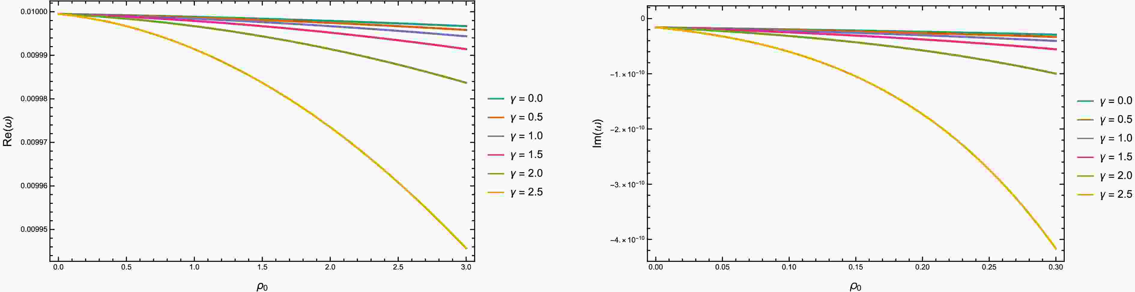
$ \mathrm{Re}(\omega) $ , while the lower panel displays the corresponding imaginary part,$ \mathrm{Im}(\omega) $ , as functions of the halo density parameter$ \rho_0 $ for several values of the inner slope parameter γ, with$ r_s=2 $ ,$ a=0.1 $ ,$ r_0=0.5 $ ,$ m=0.01 $ , and$ \ell=m_\ell=0 $ fixed. As predicted by the analytical expression in Eq. (84), increasing the halo density lowers the real part of the frequency, indicating that the scalar field becomes more tightly bound in the gravitational potential generated by the black hole and the surrounding dark matter halo. The lower panel shows that the magnitude of the imaginary part also increases with increasing$ \rho_0 $ , implying a faster decay rate. Consequently, denser and cuspier halos tend to enhance the decay while simultaneously producing more tightly bound quasibound states.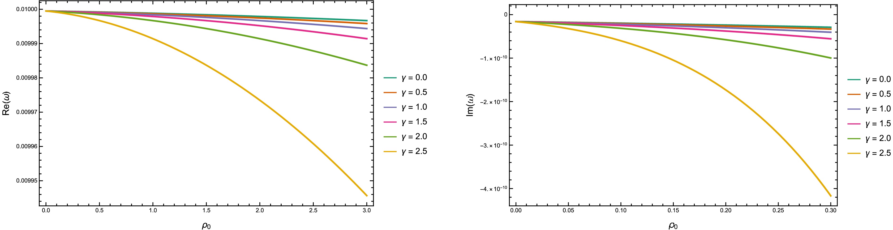
Figure 1. (color online) Profile of the quasibound state of a massive scalar field with
$ m=0.01 $ and$ \ell=m_\ell=0 $ , bound to a Kerr-Dehnen black hole with$ r_s=2 $ ,$ a=0.1 $ , and$ r_0=0.5 $ . -
We now turn to the analysis of the near-horizon region. Expanding the metric functions about the event horizon,
$ r = r_H $ , we write$ \xi(r)\simeq\xi(r_H)+\xi'(r_H)(r-r_H), $
(61) while the radial function
$ \Delta(r) $ becomes$ \Delta(r)\simeq(r-r_H)\bigl(r-r_H+2\kappa\bigr), $
(62) where
$ \kappa=r_H-\dfrac{1}{2}\xi'(r_H). $
(63) Introducing the dimensionless coordinate and frequency parameters
$ z=\dfrac{r-r_H}{2\kappa}, \qquad P=-\dfrac{\omega\xi(r_H)-a m_\ell}{2\kappa}, $
(64) the radial equation reduces to
$ z(z+1)\dfrac{{\rm d}}{{\rm d}z}\left[z(z+1)\dfrac{{\rm d}R}{{\rm d}z}\right]+\left[P^2-\lambda_\ell^{m_\ell}z(z+1)\right]R=0. $
(65) To cast the equation into hypergeometric form, we introduce the transformation
$ R(z)=\left(\dfrac{z}{z+1}\right)^{iP}Y(z), $
(66) which yields
$ z(z+1)Y''+(1+2{\rm i}P+2z)Y'-\lambda_\ell^{m_\ell}Y=0. $
(67) This is the standard hypergeometric differential equation.
The physically admissible solution is obtained by imposing purely ingoing boundary conditions at the horizon. The resulting near-horizon solution is given by (see Appendix C)
$ R_H(z)=A_1\left(\dfrac{z}{z+1}\right)^{{\rm i}P}{}_2F_1(-\ell,\ell+1,1+2{\rm i}P;-z), $
(68) where
$ A_1 $ is a normalization constant. The phase factor governed by P imposes the purely ingoing boundary condition at the event horizon. The sign of P determines the direction of the energy flux across the horizon and, therefore, whether the scalar field is absorbed or undergoes superradiant amplification.In the matching region,
$ r\gg r_H $ , the asymptotic behavior of Eq. (68) becomes$ \begin{aligned}[b] R_H(r)\approx& A_1\dfrac{\Gamma(1+2{\rm i}P)\Gamma(2\ell+1)}{\Gamma(\ell+1)\Gamma(\ell+1+2{\rm i}P)}\kappa^{-\ell}r^\ell\\ &+A_1\dfrac{\Gamma(1+2{\rm i}P)\Gamma(-2\ell-1)}{\Gamma(-\ell)\Gamma(2{\rm i}P-\ell)}\kappa^{\ell+1}r^{-\ell-1}. \end{aligned}$
(69) Matching the coefficients of the terms proportional to
$ r^\ell $ and$ r^{-\ell-1} $ with the far-region expansion in Eq. (59), we obtain$ C_1\alpha=A_1\gamma, \qquad C_1\beta\,\delta\nu=A_1\delta, $
(70) where
$\qquad\qquad \alpha = (-1)^{n_r} \dfrac{(n_r+2\ell+1)!}{(2\ell+1)!} (2k)^\ell, $
(71) $\qquad\qquad \beta = (-1)^{n_r+1} (2\ell)! \, n_r! \, (2k)^{-\ell-1}, $
(72) $\qquad\qquad \gamma = \dfrac{ \Gamma(1+2{\rm i}P)\Gamma(2\ell+1) }{ \Gamma(\ell+1)\Gamma(\ell+1+2{\rm i}P) } (2\kappa)^{-\ell}, $
(73) $\qquad\qquad \delta = \dfrac{ \Gamma(1+2{\rm i}P)\Gamma(-2\ell-1) }{ \Gamma(-\ell)\Gamma(2{\rm i}P-\ell) } (2\kappa)^{\ell+1}. $
(74) By eliminating the normalization constants
$ C_1 $ and$ A_1 $ , we obtain$ \delta\nu=\dfrac{\alpha}{\beta}\dfrac{\delta}{\gamma}. $
(75) The far-field contribution is readily evaluated as
$ \dfrac{\alpha}{\beta}=-\dfrac{(n_r+2\ell+1)!}{(2\ell+1)!(2\ell)!n_r!}(2k)^{2\ell+1}. $
(76) For the near-horizon contribution, one obtains
$ \dfrac{\delta}{\gamma}=(2\kappa)^{2\ell+1}\dfrac{\Gamma(\ell+1)}{\Gamma(2\ell+1)}\dfrac{\Gamma(-2\ell-1)}{\Gamma(-\ell)}\dfrac{\Gamma(\ell+1+2{\rm i}P)}{\Gamma(2{\rm i}P-\ell)}. $
(77) Using standard Gamma-function identities [57]
$ \qquad\dfrac{\Gamma(\ell+1+2{\rm i}P)}{\Gamma(2{\rm i}P-\ell)}=(2{\rm i}P)(-1)^\ell\prod\limits_{j=1}^{\ell}(j^2+4P^2), $
(78) $\qquad\qquad \dfrac{\Gamma(-2\ell-1)}{\Gamma(-\ell)}=(-1)^{\ell+1}\dfrac{\ell!}{(2\ell+1)!}. $
(79) Together with
$ \Gamma(\ell+1)=\ell! $ , we obtain$ \dfrac{\delta}{\gamma}=-\,2{\rm i}P\,(2\kappa)^{2\ell+1}\dfrac{(\ell!)^2}{(2\ell)!(2\ell+1)!}\prod\limits_{j=1}^{\ell}(j^2+4P^2). $
(80) Combining the contributions from the near and far regions finally yields
$\begin{aligned}[b] \delta\nu(\omega)=&2{\rm i}P\,(4k\kappa)^{2\ell+1}\dfrac{(n_r+2\ell+1)!}{n_r!}\\ &\times\left[\dfrac{\ell!}{(2\ell)!(2\ell+1)!}\right]^2\prod\limits_{j=1}^{\ell}(j^2+4P^2). \end{aligned} $
(81) Using the definitions of k and ν, together with the quantization condition, we obtain
$ m^2-\omega^2=\dfrac{A^2m^4}{4(n+\delta\nu(\omega))^2}, $
(82) where the principal quantum number is defined as
$ n=n_r+\ell+1. $
(83) Expanding perturbatively for small
$ \delta\nu $ , the bound-state spectrum is obtained as$ \omega\approx m\Bigg[1-\dfrac{A^2m^2}{8n^2}-\dfrac{A^4m^4}{128n^4}+\cdots\Bigg]+\delta\nu(m)\dfrac{A^2m^3}{4n^3}\Bigg[1+\dfrac{A^2m^2}{8n^2}+\cdots\Bigg]. $
(84) The imaginary part of the frequency originates from the factor P, implying
$ \omega_I \propto -\bigl[m\,\xi(r_H)-a m_\ell\bigr]. $
(85) The sign of this quantity determines whether the scalar mode is damped or amplified over time. Consequently, the condition for superradiant instability is
$ m\,\xi(r_H)-a m_\ell \lt 0. $
(86) In this regime, the resonant scalar modes become self-amplifying; i.e., the scalar field extracts rotational energy from the black hole through superradiant scattering, while the effective potential traps the wave, thereby forming a feedback loop. This interplay transforms the quasibound configuration into an unstable resonance that continuously extracts rotational energy from the black hole.
We now comment on the explicit role of the Dehnen halo parameters
$ (\rho_0,r_0,\gamma) $ in shaping the quasibound spectrum, the onset of superradiant instability, and the formation of scalar clouds. We note that the parameter A in (48) enters directly into the real part of the spectrum through (84).It is therefore clear that the combination
$ \rho_0 r_0^3 $ acts as an effective mass scale for the halo contribution. Increasing either$ \rho_0 $ or$ r_0 $ increases$ |A| $ , leading to a stronger binding potential and a downward shift of the energy levels. Within the physical range$ 0\leqslant \gamma <3 $ , increasing γ also enhances the magnitude of the halo correction through the factor$ (3-\gamma)^{-1} $ .Moreover, γ controls the inner slope of the density profile and thus its cuspiness. A larger γ corresponds to a more cuspy and centrally concentrated halo, which strengthens the gravitational potential in the inner region. As a result, cuspier halos produce more tightly bound quasibound states, with larger energy-level shifts and enhanced sensitivity to the dark matter parameters. Conversely, a smaller γ leads to a softer, cored profile with weaker central concentration, yielding less tightly bound quasibound states and smaller spectral deviations. It is therefore clear that cuspier halos generically support deeper and more strongly shifted QBS spectra.
For small
$ \rho_0 r_0^3 $ , the metric function admits the approximation$ f(r) \approx 1-\dfrac{r_s}{r}-\dfrac{8\pi\rho_0 r_0^3}{(3-\gamma)r}, $
(87) from which the horizon radius can be determined analytically as
$ r_H=r_s +\dfrac{ 8\pi\rho_0 r_0^3 }{3-\gamma}. $
(88) This expression explicitly shows that the halo shifts the horizon location. In particular, increasing
$ \rho_0 $ or$ r_0 $ increases$ r_H $ , thereby modifying the near-horizon geometry, where superradiant processes originate.Within the same approximation, one finds
$ \xi(r) \approx r r_s +\dfrac{8\pi r r_0^3 \rho_0}{3-\gamma}, $
(89) and
$ \xi(r_H)\approx r_s^2 + \dfrac{16\pi r_0^3 r_s \rho_0}{3-\gamma}. $
(90) It follows that the scalar cloud threshold is determined by the saturation condition
$ m\,\xi(r_H)-a m_\ell = 0, $
(91) which yields the critical scalar mass
$ m_{\rm{crit}}=\dfrac{a m_\ell}{\xi(r_H)}. $
(92) Substituting the approximate expression for
$ \xi(r_H) $ , we obtain$ m_{\rm{crit}}=\dfrac{a m_\ell}{\,r_s^2 +\dfrac{16\pi r_0^3 r_s \rho_0}{3-\gamma}\,}. $
(93) This result explicitly shows how the Dehnen halo shifts the scalar-cloud threshold relative to the Kerr case,
$ m_{\rm{crit}}^{\rm{Kerr}}=a m_\ell/r_s^2 $ . The combination$ \rho_0 r_0^3 $ controls the magnitude of the correction, while γ determines its sensitivity. For$ \gamma<3 $ , the correction increases$ \xi(r_H) $ and therefore reduces$ m_{\rm{crit}} $ , thereby narrowing the range of scalar masses that satisfy the superradiant condition.Moreover, because the growth rate is controlled by the imaginary part
$ \omega_I \propto -\left[m\,\xi(r_H)-a m_\ell\right]. $
(94) Any shift in
$ \xi(r_H) $ modifies the efficiency of energy extraction. A larger$ \rho_0 r_0^3 $ can therefore suppress or delay the onset of exponential growth, effectively weakening the instability, whereas smaller values recover the standard Kerr behavior.In summary, the Dehnen parameters
$ (\rho_0,r_0,\gamma) $ jointly control both the energy levels and the instability mechanism: they reshape the effective potential at large distances through A, while simultaneously modifying the horizon physics through$ \xi(r_H) $ . This interplay determines whether the system supports stable scalar clouds or develops a superradiant black-hole bomb.Figure 1 illustrates the dependence of the quasibound-state spectrum on the Dehnen halo parameters. The upper panel shows the real part of the frequency,
$ \mathrm{Re}(\omega) $ , while the lower panel displays the corresponding imaginary part,$ \mathrm{Im}(\omega) $ , as functions of the halo density parameter$ \rho_0 $ for several values of the inner slope parameter γ, with$ r_s=2 $ ,$ a=0.1 $ ,$ r_0=0.5 $ ,$ m=0.01 $ , and$ \ell=m_\ell=0 $ fixed. As predicted by the analytical expression in Eq. (84), increasing the halo density lowers the real part of the frequency, indicating that the scalar field becomes more tightly bound in the gravitational potential generated by the black hole and the surrounding dark matter halo. The lower panel shows that the magnitude of the imaginary part also increases with increasing$ \rho_0 $ , implying a faster decay rate. Consequently, denser and cuspier halos tend to enhance the decay while simultaneously producing more tightly bound quasibound states.
Figure 1. (color online) Profile of the quasibound state of a massive scalar field with
$ m=0.01 $ and$ \ell=m_\ell=0 $ , bound to a Kerr-Dehnen black hole with$ r_s=2 $ ,$ a=0.1 $ , and$ r_0=0.5 $ . -
While quasibound states describe the trapped, discrete sector of the spectrum, scattering modes probe the open channel through which waves interact with the rotating geometry. In this regime, the black hole behaves as an energy amplifier: incident modes can extract rotational energy and return with enhanced amplitude. This phenomenon, known as superradiant scattering, provides a direct probe of horizon physics and its modification by the surrounding dark matter halo.
In contrast to quasibound states, scattering modes correspond to unbound configurations satisfying
$ \omega \gt m, $
(95) with
$ \omega \in {\mathbb{R}} $ . Our objective is to determine how the Dehnen halo affects the amplification process. To this end, we again employ the analytical asymptotic matching (AAM) method in the low-frequency regime. -
In the asymptotic region
$ r \gg M $ , the radial equation reduces to a Coulomb-type wave equation. Introducing$ K^2 \equiv \omega^2 - m^2 \gt 0, \qquad \Lambda \equiv \dfrac{A m^2}{2K}, \qquad y = 2{\rm i}Kr, $
(96) the radial equation takes the form
$ \dfrac{{\rm d}^2}{{\rm d}y^2}(yR)+\left[-\dfrac{1}{4}+\dfrac{{\rm i}\Lambda}{y}-\dfrac{\ell(\ell+1)}{y^2}\right]yR=0. $
(97) Its general solution is
$ \begin{aligned}[b] R_\infty(y)=&B_1 {\rm e}^{-y/2} y^\ell\, {}_1F_1(\ell+1-{\rm i}\Lambda,\,2\ell+2,\,y) \\ &+ B_2 {\rm e}^{-y/2} y^{-\ell-1}\, {}_1F_1(-\ell-{\rm i}\Lambda,\,-2\ell,\,y). \end{aligned}$
(98) In the matching region (
$ y\to 0 $ ), this expression reduces to$ R_\infty \approx B_1 y^\ell + B_2 y^{-\ell-1}, $
(99) while at spatial infinity (
$ r\to\infty $ ), one obtains the asymptotic decomposition$ R_\infty(r) \approx {\cal{R}}\, {\rm e}^{+{\rm i}Kr} r^{-{\rm i}\Lambda-1} + {\cal{I}}\, {\rm e}^{-{\rm i}Kr} r^{{\rm i}\Lambda-1}, $
(100) with amplitudes
$ {\cal{R}} = \left[ B_1 \dfrac{\Gamma(2\ell+2)}{\Gamma(\ell+1-{\rm i}\Lambda)} + B_2 \dfrac{\Gamma(-2\ell)}{\Gamma(-\ell-{\rm i}\Lambda)} \right] {\left(2{\rm i}K\right)^{-{\rm i}\Lambda-1}}, $
(101) $\begin{aligned}[b] {\cal{I}} =&\Bigg[ B_1 {(-1)^{-\ell-1+{\rm i}\Lambda}}\dfrac{\Gamma(2\ell+2)}{\Gamma(\ell+1+{\rm i}\Lambda)}\\ &+ B_2 {(-1)^{\ell+{\rm i}\Lambda}}\dfrac{\Gamma(-2\ell)}{\Gamma(-\ell+{\rm i}\Lambda)} \Bigg]{(2{\rm i}K)^{-1+{\rm i}\Lambda}}. \end{aligned}$
(102) -
Near the event horizon, the physical boundary condition selects purely ingoing modes. The solution therefore retains the form
$ R_H(z)=A_1 \left(\dfrac{z}{z+1}\right)^{{\rm i}P} {}_2F_1(-\ell,\ell+1,1+2{\rm i}P;-z), $
(103) where
$ z=(r-r_H)/(2\kappa) $ and$ P = -\dfrac{\omega \xi(r_H)-a m_\ell}{2\kappa}. $
(104) In the overlap region (
$ r \gg r_H $ ), the asymptotic behavior is given by$\begin{aligned}[b] R_H(r) \approx& A_1 \dfrac{\Gamma(1+2{\rm i}P)\Gamma(2\ell+1)}{\Gamma(\ell+1)\Gamma(\ell+1+2{\rm i}P)} (2\kappa)^{-\ell} r^\ell \\ &+ A_1 \dfrac{\Gamma(1+2{\rm i}P)\Gamma(-2\ell-1)}{\Gamma(-\ell)\Gamma(2{\rm i}P-\ell)} (2\kappa)^{\ell+1} r^{-\ell-1}. \end{aligned}$
(105) Matching with the far-region expansion yields
$ \dfrac{B_2}{B_1} = (4{\rm i}\kappa K)^{2\ell+1} \dfrac{\Gamma(\ell+1)\Gamma(-2\ell-1)\Gamma(\ell+1+2{\rm i}P)} {\Gamma(2\ell+1)\Gamma(-\ell)\Gamma(2{\rm i}P-\ell)}. $
(106) -
The asymptotic structure defines the scattering coefficients, and the superradiant amplification factor is given by
$ Z = \dfrac{|{\cal{R}}|^2}{|{\cal{I}}|^2} - 1. $
(107) A positive value of Z signals amplification, indicating that the reflected wave carries more energy than the incident wave. This occurs precisely when the horizon flux is negative.
The superradiant condition follows directly from the near-horizon parameter P, namely
$ \omega \,\xi(r_H) - a m_\ell \lt 0, $
(108) which generalizes the Kerr condition by incorporating the dark matter contribution through
$ \xi(r_H) $ .This immediately implies that the superradiant cutoff frequency is given by
$ \omega_c = \dfrac{a m_\ell}{\xi(r_H)}, $
(109) so that amplification occurs for
$ \omega \lt \omega_c $ . The effect of the Dehnen halo parameters$ (\rho_0, r_0, \gamma) $ is therefore fully encoded in the behavior of$ \xi(r_H) $ .Using the small-halo approximation
$ \xi(r_H)\approx r_s^2 + \dfrac{16\pi r_0^3 r_s \rho_0}{3-\gamma}, $
(110) one can identify the following effects.
First, the combination
$ \rho_0 r_0^3 $ controls the magnitude of the deviation from the Kerr value,$ \xi_{\rm{Kerr}}=r_s^2 $ . Increasing either$ \rho_0 $ or$ r_0 $ enhances this correction. For$ \gamma<3 $ , the denominator$ (3-\gamma) $ is negative, so the correction increases$ \xi(r_H) $ , which in turn lowers the cutoff frequency$ \omega_c $ . As a result, the superradiant window$ \omega<\omega_c $ becomes narrower, suppressing the amplification efficiency.Second, the parameter γ regulates the strength of this effect through the factor
$ (3-\gamma)^{-1} $ . As γ increases, the correction becomes increasingly large, leading to a significant increase in$ \xi(r_H) $ and a corresponding reduction in$ \omega_c $ . Physically, larger values of γ correspond to cuspier and more centrally concentrated halos, which increase the halo correction to the near-horizon geometry. This increases$ \xi(r_H) $ , thereby reducing the horizon angular velocity$ a/\xi(r_H) $ and lowering the superradiant cutoff frequency.Finally, this behavior admits a clear physical interpretation: an increase in
$ \xi(r_H) $ reduces the horizon angular velocity$ a/\xi(r_H) $ , thereby lowering the superradiant cutoff frequency and suppressing the amplification of incident waves. Conversely, for smaller$ \rho_0 r_0^3 $ and less cuspy halos, the correction becomes negligible and the standard Kerr result is smoothly recovered, with a wider superradiant window.Figure 2 illustrates the superradiant amplification factor Z as a function of the scalar-field frequency for several values of the Dehnen inner slope parameter γ, with all other parameters held fixed. In all cases, amplification occurs only within the superradiant regime, reaches a maximum, and then decreases to zero at the cutoff frequency
$ \omega_c $ . As γ increases, the peak amplification is systematically reduced, and the frequency interval over which$ Z>0 $ becomes progressively narrower. This behavior is consistent with the analytical results obtained above. A larger value of γ increases$ \xi(r_H) $ and consequently decreases the effective horizon angular velocity,$ a/\xi(r_H) $ . As a result, the superradiant threshold shifts to lower frequencies, reducing the efficiency of rotational energy extraction and suppressing the amplification of the scattered scalar waves. In the limit$ \gamma\to 0 $ , the halo correction becomes very weak, and the amplification profile approaches the Kerr behavior, i.e.$ \Omega_H=a/ (r_H^2+a^2)=0.02375 $ .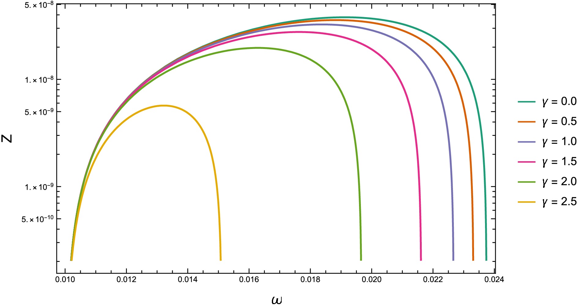
Figure 2. (color online) Amplification factor profile of a massive scalar field with
$ m=0.01 $ and$ \ell=m_\ell=+1 $ , bound to a Kerr-Dehnen black hole with$ r_s=2 $ ,$ a=0.1 $ ,$ \rho_0=0.1 $ , and$ r_0=0.5 $ . -
The asymptotic structure defines the scattering coefficients, and the superradiant amplification factor is given by
$ Z = \dfrac{|{\cal{R}}|^2}{|{\cal{I}}|^2} - 1. $
(107) A positive value of Z signals amplification, indicating that the reflected wave carries more energy than the incident wave. This occurs precisely when the horizon flux is negative.
The superradiant condition follows directly from the near-horizon parameter P, namely
$ \omega \,\xi(r_H) - a m_\ell \lt 0, $
(108) which generalizes the Kerr condition by incorporating the dark matter contribution through
$ \xi(r_H) $ .This immediately implies that the superradiant cutoff frequency is given by
$ \omega_c = \dfrac{a m_\ell}{\xi(r_H)}, $
(109) so that amplification occurs for
$ \omega \lt \omega_c $ . The effect of the Dehnen halo parameters$ (\rho_0, r_0, \gamma) $ is therefore fully encoded in the behavior of$ \xi(r_H) $ .Using the small-halo approximation
$ \xi(r_H)\approx r_s^2 + \dfrac{16\pi r_0^3 r_s \rho_0}{3-\gamma}, $
(110) one can identify the following effects.
First, the combination
$ \rho_0 r_0^3 $ controls the magnitude of the deviation from the Kerr value,$ \xi_{\rm{Kerr}}=r_s^2 $ . Increasing either$ \rho_0 $ or$ r_0 $ enhances this correction. For$ \gamma<3 $ , the denominator$ (3-\gamma) $ is negative, so the correction increases$ \xi(r_H) $ , which in turn lowers the cutoff frequency$ \omega_c $ . As a result, the superradiant window$ \omega<\omega_c $ becomes narrower, suppressing the amplification efficiency.Second, the parameter γ regulates the strength of this effect through the factor
$ (3-\gamma)^{-1} $ . As γ increases, the correction becomes increasingly large, leading to a significant increase in$ \xi(r_H) $ and a corresponding reduction in$ \omega_c $ . Physically, larger values of γ correspond to cuspier and more centrally concentrated halos, which increase the halo correction to the near-horizon geometry. This increases$ \xi(r_H) $ , thereby reducing the horizon angular velocity$ a/\xi(r_H) $ and lowering the superradiant cutoff frequency.Finally, this behavior admits a clear physical interpretation: an increase in
$ \xi(r_H) $ reduces the horizon angular velocity$ a/\xi(r_H) $ , thereby lowering the superradiant cutoff frequency and suppressing the amplification of incident waves. Conversely, for smaller$ \rho_0 r_0^3 $ and less cuspy halos, the correction becomes negligible and the standard Kerr result is smoothly recovered, with a wider superradiant window.Figure 2 illustrates the superradiant amplification factor Z as a function of the scalar-field frequency for several values of the Dehnen inner slope parameter γ, with all other parameters held fixed. In all cases, amplification occurs only within the superradiant regime, reaches a maximum, and then decreases to zero at the cutoff frequency
$ \omega_c $ . As γ increases, the peak amplification is systematically reduced, and the frequency interval over which$ Z>0 $ becomes progressively narrower. This behavior is consistent with the analytical results obtained above. A larger value of γ increases$ \xi(r_H) $ and consequently decreases the effective horizon angular velocity,$ a/\xi(r_H) $ . As a result, the superradiant threshold shifts to lower frequencies, reducing the efficiency of rotational energy extraction and suppressing the amplification of the scattered scalar waves. In the limit$ \gamma\to 0 $ , the halo correction becomes very weak, and the amplification profile approaches the Kerr behavior, i.e.$ \Omega_H=a/ (r_H^2+a^2)=0.02375 $ .
Figure 2. (color online) Amplification factor profile of a massive scalar field with
$ m=0.01 $ and$ \ell=m_\ell=+1 $ , bound to a Kerr-Dehnen black hole with$ r_s=2 $ ,$ a=0.1 $ ,$ \rho_0=0.1 $ , and$ r_0=0.5 $ . -
We explored the dynamics of scalar fields in a rotating black hole spacetime dressed by a Dehnen dark matter halo, focusing on how quasibound states and superradiant scattering combine to determine the full spectral response of the system. Starting from a consistent rotating geometry constructed via the Newman–Janis algorithm, we formulated the Klein–Gordon equation and employed the analytical asymptotic matching (AAM) method to connect the near-horizon and asymptotic regions. This approach provides a unified analytic framework in which both trapped modes and scattering processes emerge naturally from the same underlying structure.
In the quasibound regime, we derived an explicit analytical expression for the complex frequency spectrum, clearly identifying its physical origin. The real part is governed by the asymptotic far-region behavior and retains a hydrogen-like structure, now shifted by the presence of the dark matter halo through the parameter
$ A=-r_s-\dfrac{8\pi \rho_0 r_0^3}{3-\gamma} $ , which parameterizes the leading-order halo correction to the far-region gravitational potential. Increasing either$ \rho_0 $ or$ r_0 $ deepens the effective potential and shifts the energy levels downward, leading to more tightly bound scalar clouds. The parameter γ, which controls the inner slope of the density profile, further modulates this effect: larger γ corresponds to cuspier and more centrally concentrated halos, enhancing the binding and producing more pronounced deviations from the vacuum spectrum. By contrast, smaller γ yields softer, more diffuse halos with weaker spectral shifts.The imaginary part of the frequency arises entirely from the near-horizon dynamics and encodes the exchange of energy with the rotating black hole. This contribution depends on the quantity
$ \xi(r_H) $ , which is also modified by the halo parameters. Consequently, the black hole bomb condition is deformed by the halo-dependent geometry, shifting the threshold for instability and the formation of scalar clouds. In particular, increasing$ \rho_0 $ or$ r_0 $ , or considering more cuspy profiles (larger γ), reduces the critical mass required for instability and typically suppresses the growth rate.In the scattering sector, we obtained an analytical expression for the superradiant amplification factor Z by explicitly matching ingoing and outgoing modes at infinity. The dark matter halo modifies the effective potential experienced by the scalar field, leading to changes in both the phase evolution and the amplification efficiency. The superradiant condition is correspondingly altered to
$ \omega \xi(r_H) - a m_\ell \lt 0 $ , demonstrating that the extraction of rotational energy is directly sensitive to the surrounding matter distribution. Through$ \xi(r_H) $ , the parameters$ \rho_0 $ ,$ r_0 $ , and γ shift the cutoff frequency and typically narrow the superradiant window, with denser, larger, and more cuspy halos reducing the amplification efficiency relative to the Kerr case.Taken together, quasibound states and superradiant scattering are not separate phenomena but two complementary facets of the same spectral structure. The far region determines the quasibound-state spectrum, while the near-horizon region governs its growth, decay, and superradiant amplification. The presence of the Dehnen halo acts as an environmental tuner, with
$ \rho_0 $ and$ r_0 $ setting the overall strength of the effect and γ controlling its radial stiffness. In this way, the spectrum and scattering properties of a rotating black hole provide a potential probe of the surrounding Dehnen dark matter environment. -
A second-order ordinary differential equation can be cast into normal (Schrödinger-like) form by eliminating the first-derivative term. This representation is particularly useful for qualitative and asymptotic analyses [58].
Consider the linear equation
$ \dfrac{{\rm d}^2 y}{{\rm d}x^2}+p(x)\dfrac{{\rm d}y}{{\rm d}x}+q(x)y=0. $
(A1) To remove the first-derivative term, we introduce the transformation
$ y(x)=Y(x)\exp \left(-\dfrac{1}{2}\int p(x)\,{\rm d}x\right), $
(A2) which is chosen such that the resulting equation for
$ Y(x) $ contains no$ {\rm d}Y/{\rm d}x $ term [59]. Substituting this into Eq. (111), we obtain$ \dfrac{{\rm d}^2 Y}{{\rm d}x^2} +\left( -\dfrac{1}{2}\dfrac{{\rm d}p}{{\rm d}x} -\dfrac{1}{4}p^2 +q \right)Y=0. $
(A3) Defining
$ Q(x)=-\dfrac{1}{2}\dfrac{{\rm d}p}{{\rm d}x}-\dfrac{1}{4}p^2+q, $
(A4) Eq. (A3) can be written in the compact form
$ \dfrac{{\rm d}^2 Y}{{\rm d}x^2}=-Q(x)Y. $
(A5) This representation provides immediate qualitative insight. If
$ Q(x)>0 $ , the solution is locally oscillatory and necessarily crosses the x-axis. Moreover, if$ \int^{\infty} Q(x)\,{\rm d}x = \infty, $
(A6) then
$ Y(x) $ has infinitely many zeros [59]. In contrast, if$ Q(x)<0 $ , the solution is nonoscillatory and has at most one zero. -
The confluent hypergeometric equation arises as a canonical normal form in a broad class of radial problems. It can be written as [60]
$ \dfrac{{\rm d}^2\psi_C}{{\rm d}x^2}+\left(-\dfrac{1}{4}+\dfrac{k}{x}+\dfrac{\dfrac{1}{4}-m^2}{x^2}\right)\psi_C=0, $
(B1) which is recognized as the Whittaker equation.
Its general solution is given by
$ \psi_C=A\,M_{k,m}(x)+B\,M_{k,-m}(x), $
(B2) where A and B are constants. The Whittaker functions are related to the confluent hypergeometric function
$ {}_1F_1 $ as follows:$ M_{k,\pm m}(x) = x^{\tfrac{1}{2}\pm m} {\rm e}^{-\tfrac{x}{2}} {}_1F_1 \left( \dfrac{1}{2}-k\pm m, 1\pm 2m, x \right). $
(B3) The power-law prefactor controls the behavior near the origin, whereas the exponential factor governs the asymptotic behavior for large x. For
$ |x|\to\infty $ , one has [58]$\begin{aligned}[b] {}_1F_1(a,b,x)=&\dfrac{\Gamma(b)}{\Gamma(a)}{\rm e}^{x}x^{a-b} {}_2F_0\left(b-a,1-a;-\dfrac{1}{x}\right)\\ &+\dfrac{\Gamma(b)}{\Gamma(b-a)}(-x)^{-a} {}_2F_0\left(a,a-b+1;-\dfrac{1}{x}\right). \end{aligned} $
(B4) -
The Gauss hypergeometric equation is the prototypical second-order equation with three regular singular points [60]
$\begin{aligned}[b] x(1-x)\dfrac{{\rm d}^2\psi_G}{{\rm d}x^2}+\left[a_3-(a_1+a_2+1)x\right]\dfrac{{\rm d}\psi_G}{{\rm d}x}-a_1a_2\psi_G=0. \end{aligned}$
(C1) Its general solution is
$\begin{aligned}[b] \psi_G=&A\,{}_2F_1(a_1,a_2,a_3,x)\\ &+B\,x^{1-a_3}{}_2F_1(a_1-a_3+1,a_2-a_3+1,2-a_3,x), \end{aligned} $
(C2) where A and B are constants.
As shown in Appendix A, Eq. (C1) can be cast into normal form by defining
$ \Psi_G=x^{\tfrac{a_3}{2}}(1-x)^{\tfrac{1}{2}(1+a_1+a_2-a_3)}\psi_G, $
(C3) which yields
$ \dfrac{{\rm d}^2\Psi_G}{{\rm d}x^2}-V_{\rm{eff}}(x)\Psi_G=0, $
(C4) with
$\begin{aligned}[b] V_{\rm{eff}}(x)=&\\ &\dfrac{x^2 \left((a_1 - a_2)^2 - 1\right) - 2x \left((a_1 + a_2 - 1)a_3 - 2a_1a_2\right) + a_3(a_3 - 2)}{4x^2(1 - x)^2}. \end{aligned}$
(C5) This form makes the singular behavior at
$ x=0 $ and$ x=1 $ explicit.We now consider the modified equation
$ x(1+x)\dfrac{{\rm d}^2\psi_G}{{\rm d}x^2}+(2x+1)\dfrac{{\rm d}\psi_G}{{\rm d}x} +\left(\dfrac{{\cal{A}}}{x}-\dfrac{{\cal{B}}}{x+1}+{\cal{C}}\right)\psi_G=0, $
(C6) which can be transformed into the standard hypergeometric form through a change of variables.
Its general solution is given by
$\begin{aligned}[b] \psi_G=&(x+1)^{-{\rm i}\sqrt{{\cal{B}}}} \Big[ A\,x^{{\rm i}\sqrt{{\cal{A}}}}{}_2F_1({\cal{A}}_1,{\cal{A}}_2,{\cal{A}}_3,-x)\\ & +B\,x^{-{\rm i}\sqrt{{\cal{A}}}}{}_2F_1({\cal{A}}_4,{\cal{A}}_5,{\cal{A}}_6,-x) \Big], \end{aligned}$
(C7) where the parameters are
$ {\cal{A}}_1 = \dfrac{1}{2}\left(1+\sqrt{1-4{\cal{C}}}\right) +{\rm i}\left(\sqrt{{\cal{A}}}-\sqrt{{\cal{B}}}\right), $
(C8) $ {\cal{A}}_2 = \dfrac{1}{2}\left(1-\sqrt{1-4{\cal{C}}}\right) +{\rm i}\left(\sqrt{{\cal{A}}}-\sqrt{{\cal{B}}}\right), $
(C9) $ {\cal{A}}_3 = 1+2{\rm i}\sqrt{{\cal{A}}}, $
(C10) $ {\cal{A}}_4 = \dfrac{1}{2}\left(1+\sqrt{1-4{\cal{C}}}\right) -{\rm i}\left(\sqrt{{\cal{A}}}+\sqrt{{\cal{B}}}\right), $
(C11) $ {\cal{A}}_5 = \dfrac{1}{2}\left(1-\sqrt{1-4{\cal{C}}}\right) -{\rm i}\left(\sqrt{{\cal{A}}}+\sqrt{{\cal{B}}}\right), $
(C12) $ {\cal{A}}_6 = 1-2{\rm i}\sqrt{{\cal{A}}}. $
(C13) A key ingredient in asymptotic matching is the analytic continuation of
$ {}_2F_1 $ to large arguments. The connection formula is given by$ \begin{aligned}[b] {}_2F_1(a_1,a_2,a_3,x)= &\dfrac{\Gamma(a_2-a_1)\Gamma(a_3)}{\Gamma(a_2)\Gamma(a_3-a_1)}(-x)^{-a_1} {}_2F_1\\ & \times \left(a_1,a_1-a_3+1,a_1-a_2+1,\dfrac{1}{x}\right)\\ & +\dfrac{\Gamma(a_1-a_2)\Gamma(a_3)}{\Gamma(a_1)\Gamma(a_3-a_2)}(-x)^{-a_2} {}_2F_1 \\ & \times \left(a_2,a_2-a_3+1,a_2-a_1+1,\dfrac{1}{x}\right), \end{aligned}$
(C14) which is the primary tool used to extract the large-x behavior of the near-horizon solution in the main text.
-
The Gauss hypergeometric equation is the prototypical second-order equation with three regular singular points [60]
$\begin{aligned}[b] x(1-x)\dfrac{{\rm d}^2\psi_G}{{\rm d}x^2}+\left[a_3-(a_1+a_2+1)x\right]\dfrac{{\rm d}\psi_G}{{\rm d}x}-a_1a_2\psi_G=0. \end{aligned}$
(C1) Its general solution is
$\begin{aligned}[b] \psi_G=&A\,{}_2F_1(a_1,a_2,a_3,x)\\ &+B\,x^{1-a_3}{}_2F_1(a_1-a_3+1,a_2-a_3+1,2-a_3,x), \end{aligned} $
(C2) where A and B are constants.
As shown in Appendix A, Eq. (C1) can be cast into normal form by defining
$ \Psi_G=x^{\tfrac{a_3}{2}}(1-x)^{\tfrac{1}{2}(1+a_1+a_2-a_3)}\psi_G, $
(C3) which yields
$ \dfrac{{\rm d}^2\Psi_G}{{\rm d}x^2}-V_{\rm{eff}}(x)\Psi_G=0, $
(C4) with
$\begin{aligned}[b] V_{\rm{eff}}(x)=&\\ &\dfrac{x^2 \left((a_1 - a_2)^2 - 1\right) - 2x \left((a_1 + a_2 - 1)a_3 - 2a_1a_2\right) + a_3(a_3 - 2)}{4x^2(1 - x)^2}. \end{aligned}$
(C5) This form makes the singular behavior at
$ x=0 $ and$ x=1 $ explicit.We now consider the modified equation
$ x(1+x)\dfrac{{\rm d}^2\psi_G}{{\rm d}x^2}+(2x+1)\dfrac{{\rm d}\psi_G}{{\rm d}x} +\left(\dfrac{{\cal{A}}}{x}-\dfrac{{\cal{B}}}{x+1}+{\cal{C}}\right)\psi_G=0, $
(C6) which can be transformed into the standard hypergeometric form through a change of variables.
Its general solution is given by
$\begin{aligned}[b] \psi_G=&(x+1)^{-{\rm i}\sqrt{{\cal{B}}}} \Big[ A\,x^{{\rm i}\sqrt{{\cal{A}}}}{}_2F_1({\cal{A}}_1,{\cal{A}}_2,{\cal{A}}_3,-x)\\ & +B\,x^{-{\rm i}\sqrt{{\cal{A}}}}{}_2F_1({\cal{A}}_4,{\cal{A}}_5,{\cal{A}}_6,-x) \Big], \end{aligned}$
(C7) where the parameters are
$ {\cal{A}}_1 = \dfrac{1}{2}\left(1+\sqrt{1-4{\cal{C}}}\right) +{\rm i}\left(\sqrt{{\cal{A}}}-\sqrt{{\cal{B}}}\right), $
(C8) $ {\cal{A}}_2 = \dfrac{1}{2}\left(1-\sqrt{1-4{\cal{C}}}\right) +{\rm i}\left(\sqrt{{\cal{A}}}-\sqrt{{\cal{B}}}\right), $
(C9) $ {\cal{A}}_3 = 1+2{\rm i}\sqrt{{\cal{A}}}, $
(C10) $ {\cal{A}}_4 = \dfrac{1}{2}\left(1+\sqrt{1-4{\cal{C}}}\right) -{\rm i}\left(\sqrt{{\cal{A}}}+\sqrt{{\cal{B}}}\right), $
(C11) $ {\cal{A}}_5 = \dfrac{1}{2}\left(1-\sqrt{1-4{\cal{C}}}\right) -{\rm i}\left(\sqrt{{\cal{A}}}+\sqrt{{\cal{B}}}\right), $
(C12) $ {\cal{A}}_6 = 1-2{\rm i}\sqrt{{\cal{A}}}. $
(C13) A key ingredient in asymptotic matching is the analytic continuation of
$ {}_2F_1 $ to large arguments. The connection formula is given by$ \begin{aligned}[b] {}_2F_1(a_1,a_2,a_3,x)= &\dfrac{\Gamma(a_2-a_1)\Gamma(a_3)}{\Gamma(a_2)\Gamma(a_3-a_1)}(-x)^{-a_1} {}_2F_1\\ & \times \left(a_1,a_1-a_3+1,a_1-a_2+1,\dfrac{1}{x}\right)\\ & +\dfrac{\Gamma(a_1-a_2)\Gamma(a_3)}{\Gamma(a_1)\Gamma(a_3-a_2)}(-x)^{-a_2} {}_2F_1 \\ & \times \left(a_2,a_2-a_3+1,a_2-a_1+1,\dfrac{1}{x}\right), \end{aligned}$
(C14) which is the primary tool used to extract the large-x behavior of the near-horizon solution in the main text.
Tuning a rotating black hole spectrum with dark matter halo: quasibound states, scalar cloud, black hole bomb and superradiant scattering
- Received Date: 2026-06-11
- Available Online: 2026-11-15
Abstract: We investigate the spectral dynamics of a rotating black hole embedded in a Dehnen $(1,4,\gamma)$ dark matter halo, in which quasibound states and superradiant scattering jointly characterize the physical response of the system. Starting from an exact Schwarzschild–Dehnen solution, we construct its rotating counterpart via the Newman–Janis algorithm, thereby obtaining a consistent axisymmetric geometry that incorporates the influence of a structured halo. Through its inner slope parameter γ, the Dehnen profile introduces a controlled deformation of both the near-horizon and asymptotic regions of the spacetime. Using the analytical asymptotic matching method, we derive the quasibound-state spectrum and show that the real part of the frequency retains a hydrogen-like structure but is systematically shifted by the leading-order halo correction proportional to $\rho_0 r_0^3/(3-\gamma)$. In particular, denser, more extended, and cuspier halos strengthen the binding of the quasibound states, lower the critical mass required for the onset of instability, and typically suppress the growth rate of the black hole bomb. In the scattering sector, we obtain an analytic expression for the superradiant amplification factor and find that the same halo properties that strengthen the binding effects also tend to narrow the superradiant window. These results demonstrate that quasibound states and superradiant scattering are complementary manifestations of a unified spectral structure, with the Dehnen halo acting as an environmental tuner that directly imprints its properties onto both the resonance spectrum and the energy-extraction channels of the rotating black hole.



 DownLoad: