


 Abstract
 HTML
 Reference
 Related
 PDF




-
Quantum Chromodynamics (QCD) is a theory of color forces among quarks and gluons. It exhibits two distinct features in opposite energy regimes. On the one hand, it exhibits asymptotic freedom [1, 2] in the high-energy domain, where perturbative methods based on Feynman diagrams are useful for describing strong interactions [3]. At low energies, on the other hand, QCD becomes highly non-linear because the strong coupling
$ \alpha_s $ rightfully deserves its name (see, for instance, Ref. [4] and references therein), rendering any perturbative attempt to describe strong interactions ineffective in this regime. Non-perturbative tools such as lattice QCD [5] (see also references therein), Schwinger-Dyson equations (SDEs) [6] (see references therein), and other effective approaches [7] are required to properly account for the hadronization of the fundamental degrees of freedom of the theory. The latter is a process that depends strongly on the properties of the quark and gluon environment, namely temperature, density, and the influence of external magnetic fields, for instance. The vanishing of the dynamical component of the quark masses at small or vanishing baryon chemical potential and at temperatures around 150−170 MeV, corresponding to chiral symmetry restoration, can be studied from the behavior of the chiral condensate in lattice QCD [8] and continuum studies [9−12]. Nevertheless, the melting of hadrons into the quark–gluon plasma (see, for instance, Refs. [13−15] and references therein) –corresponding to a cross-over between the confinement and deconfinement phases of quark matter with physical current quark mass– has commonly been studied in lattice simulations through the behavior of the Polyakov loop (PL) [16]. The quark–antiquark condensate is an exact order parameter for chiral symmetry breaking/restoration in the chiral limit ($ m\rightarrow0 $ where m represents the current quark mass). At finite temperature T, the chiral transition is of second order for the light quark flavors$ N_{f} = 2 $ in the chiral limit, whereas it is first order for two light and one heavy quark flavors$ N_f = 2+1 $ . Here, the chiral condensate serves as a genuine order parameter. In lattice QCD, the confinement/deconfinement phase transition in the chiral limit can be characterized by the Polyakov loop. The Polyakov loop is a fundamental lattice gauge theory operator used to probe the deconfinement transition in finite-temperature QCD, especially in the pure gauge sector, where it serves as an order parameter for confinement under the$ Z(N_c) $ center symmetry [17, 18]. Its logarithm is proportional to the negative of the static-quark free energy in units of temperature. Since the Polyakov loop is not invariant under$ Z(N_c) $ transformations, it vanishes below the transition temperature (static-quark free energy diverges) and becomes finite above the transition temperature$ T_c $ due to color screening [18, 19]. Thus, the deconfinement transition is tied to the onset of screening. In full QCD, sea quarks explicitly break center symmetry: when a string between a color charge pair breaks, a light quark–antiquark pair is created, giving the Polyakov loop a small, positive expectation value in the confined phase and complicating its role as a strict order parameter. Consequently, deconfinement in QCD is often discussed through fluctuations of conserved charges rather than solely via the Polyakov loop [19].The clear physical interpretation of the Polyakov loop as the free energy of a single quark makes it a preferred order parameter for coupling to effective models based on the Nambu–Jona-Lasinio (NJL) [20] model, which lacks confinement, forming PNJL models in which chiral dynamics is coupled to a Polyakov loop potential to mimic confinement [21]. Between the chiral and infinite quark mass limits, there is a crossover region where neither the quark condensate nor the Polyakov loop is an exact order parameter; thus, they signal only smooth transitions. Nevertheless, both quantities remain interesting objects of investigation. Numerical simulations in lattice QCD indicate that the critical temperature
$ T_c $ is the same for both transitions (chiral symmetry restoration and deconfinement). Thus, it is widely believed that there must be a mechanism linking the two phenomena [22]. However, so far, there is no generally accepted picture for such a link. The dressed Polyakov loop, often denoted$ \Sigma_{I} $ , is a related ''dual'' observable that combines the usual Polyakov loop with information from the Dirac operator spectrum. It acts as a novel order parameter for the deconfinement transition and connects to chiral symmetry breaking (see [22−25]) and is expected to be useful in functional approaches. A new approach to relating Dirac eigenvalues to confinement was proposed [22], showing that the Polyakov loop can be written as a linear combination of spectral sums of Dirac eigenvalues computed with different fermionic boundary conditions. In the quenched limit, the Polyakov loop is an order parameter for confinement, vanishing in the confined phase and acquiring a nonzero expectation value above$ T_c $ in the deconfinement phase. The proposed framework suggests that the distinction between phases may arise from the differential response of the Dirac spectrum to changes in the boundary conditions [22].Functional approaches, including renormalization-group equations (RG) and Schwinger–Dyson equation methods, do not directly or readily yield confinement/deconfinement order parameters. Ref. [26] introduced a procedure to test confinement by deriving the Polyakov-loop potential, suggesting its use as an order parameter for the transition. Meanwhile, the dressed Polyakov loop (also known as the dual quark condensate) has been proposed as an order parameter for the confinement–deconfinement transition within the Schwinger–Dyson formalism [27−30].
However, a natural way to understand the characteristics of confinement is provided by the infrared behavior of Green functions of quarks and gluons [31]. The analytic properties of these propagators have been used in several ways to test confinement-deconfinement in QCD [32, 33]; they remain valid tools, and these properties can naturally be explored in other QCD-like theories as well. A symmetry-preserving contact interaction (CI) model for quarks [34] is based on a momentum-independent truncation of the Schwinger-Dyson equations, with a regularization scheme that ensures that the quark propagator remains free of real or complex poles. In this context, confinement is achieved by introducing an infrared cutoff
$ \tau_{ir} = 1/\Lambda_{ir} $ in addition to an ultraviolet cutoff$ \tau_{uv} = 1/\Lambda_{uv} $ [35]. The infrared cutoff serves to eliminate unphysical thresholds and plays a crucial role in enforcing confinement. The absence of poles in the quark propagator is indicative of a confined excitation within the framework of axiomatic field theory [35]. This approach maintains the symmetry of the system while ensuring the physical consistency of the model. The CI (or NJL) model does not account for gauge boson mediation, so there is no center symmetry and one cannot associate the Polyakov or dressed Polyakov loops [36]. Therefore, arguments for confinement based on the vacuum expectation values of these quantities are not applicable in this scenario. The confinement scale ($ \tau_{ir} $ at zero and finite T, at density μ, in background fields, and under screening from a large number of light quark flavors$ N_f $ ) can serve as an order parameter for the confinement-deconfinement transition [37−44]. It is worth noting that, in the chiral limit, the confinement length scale remains finite, indicating confinement, up to the critical temperature$ T_c $ ; above this temperature, the model transitions to the ordinary NJL model, resulting in the emergence of poles in the propagator and an anticipated deconfinement transition [37−44]. In the confined phase, the quark propagator does not exhibit pole singularities, whereas in the deconfined phase, there may be multiple or even a single pole singularity, as indicated by a study of the non-local NJL model [45].While lattice QCD provides a first-principles numerical approach, the functional methods discussed here offer a unique window into the analytic structure of the theory. It is important to distinguish between indicators that are theoretically fundamental, such as the Polyakov loop in the pure-gauge limit, and those that serve as model-dependent proxies, such as the infrared regularization scales in contact interaction models.
This review aims to provide a pedagogical overview for both experts and non-experts, focusing on the transition between different regimes of QCD. By comparing continuum functional methods with effective models, we highlight the strengths and inherent limitations of various confinement indicators. In this work, we present a survey of different parameters that have been used to test confinement through the analytic properties of the quark propagator in QCD and various effective models. We describe how these parameters have been extended to finite temperature and other environments with some degree of success. We have organized the work as follows: We review the basics of QCD in Sec. II, with particular attention to the analytic structure of the quark propagator. We then review some of the more successful models that have been employed within the SDEs framework to describe chiral symmetry breaking and confinement in QCD in Sec. III. The axiom of reflection positivity and its implications for confinement are presented in Sec. IV, and the dressed Polyakov loop (dPL) is discussed in Sec. V. The summary and perspectives are finally presented in Sec. VII.
-
Quantum chromodynamics (QCD) is a well-established theory of strong color interactions in the Standard Model of particle physics. On the basis of gauge-symmetry arguments, the corresponding Lagrangian is expressed as [3]:
$ {\cal{L}}_{\rm QCD} = \sum^{3}\limits_{a = 1}\sum^{N_{f}}\limits_{A = 1}\bar{\psi}^{A}_{a}\left({\rm i}\gamma^{\mu}D_{\mu}-m_{A} \right)\psi^{A}_{a}-\frac{1}{4} F^{s}_{\mu\nu}F^{s\mu\nu} . $
(1) The first term in Eq. (1) represents the quark sector, where ψ and
$ \bar{\psi} $ denote the quark and antiquark fields, respectively. Each of the$ N_f $ flavors has current quark mass$ m_{A} $ , and a denotes a color index. The second term represents the gauge sector, with$ F^{s}_{\mu\nu} = \partial_{\mu}G^{s}_{\nu}-\partial_{\nu}G^{s}_{\mu}- g_{s}f_{stu} G^{t}_{\mu}G^{u}_{\nu}\;, $
(2) corresponding to the gauge field strength tensor, defined in terms of the covariant derivative
$ D_\mu \psi^{A}_{b} = \partial_\mu \psi^{A}_{a}+\frac{{\rm i}g_{s}}{2}G^{t}_{\mu}(\lambda^{t})_{ab}\psi^{A}_{b} $
(3) as the commutator
$ [D_\mu,D_\nu] = -{\rm i}g_s \frac{\lambda^a}{2}F_{\mu\nu}^a\;. $
(4) In this context,
$ g_{s} $ denotes the QCD coupling, while$ \lambda^{\alpha} $ denotes the Gell-Mann matrices, with internal indices$ s, t, u $ running from 1 to 8. These matrices satisfy the$S U(3)$ Lie algebra$ [\lambda_s, \lambda_t] = 2{\rm i}f_{stu} \lambda_u, $
(5) where
$ f_{stu} $ denote the$S U(3)$ structure constants,$ \begin{split} f_{123} &= 1,\\ f_{147} &= -f_{156} = f_{246} = f_{257} = f_{345} = -f_{367} = \frac{1}{2}, \\ f_{458} &= f_{678} = \frac{\sqrt{3}}{2}, \end{split} $
(6) whereas the remaining
$ f_{abc} $ that are not related to those above by permutations vanish.In the real world, there are eight gluon fields, denoted by
$ G^{t}_{\mu} $ , and six flavors of quarks, each of which exists in three color states: red, green, or blue. The QCD Lagrangian retains the flavor symmetries of a free-quark model, with nondegenerate quark masses as the only source of symmetry breaking. It is also invariant under charge conjugation and space inversion. In this work, we focus on the chiral symmetry of the Lagrangian. This chiral symmetry is described by the special unitary group$S U(2)_L \otimes S U(2)_R$ . Introducing the left- and right-handed fermion fields through the projectors$ \psi_{L} = (1-\gamma^5)\psi/2 $ and$ \psi_{R} = (1+\gamma^5)\psi/2 $ , for$ N_f = 2 $ , the Dirac part of the QCD Lagrangian in Eq. (1) can be written as:$ \begin{split} {\cal{L}}_{\rm QCD} =\;& \bar{\psi}^{u,d}_{L}\left({\rm i}\not{\,D}\right)\psi^{u,d}_{L}+\bar{\psi}^{u,d}_{R}\left({\rm i}\not{\,D}\right)\psi^{u,d}_{R} \\&-\bar{\psi}^{u,d}_{L}\left(m_{u,d} \right)\psi^{u,d}_{R}- \bar{\psi}^{u,d}_{R}\left(m_{u,d}\right)\psi^{u,d}_{L}. \end{split} $
(7) For massless up and down quarks (
$ m_{u} = m_{d} = m_A = 0 $ ), the Lagrangian is invariant under the following gauge transformations:$ \psi_{R}\rightarrow {\rm{Exp}}[{-{\rm i}\vec{\sigma}\cdot \vec{\theta}_{R}}] \psi_{R}, \qquad \psi_{L}\rightarrow {\rm{Exp}}[-{\rm i}\vec{\sigma}\cdot \vec{\theta}_{L}] \psi_{L}. $
(8) When
$ m_u = m_d = m_A\neq0 $ , the QCD Lagrangian is no longer chirally symmetric because the mass term$ \bar{\psi}m_{u,d}\psi $ explicitly breaks chiral symmetry. In the vacuum, the chiral symmetry$S U(2)_L \otimes S U(2)_R$ is also spontaneously broken by a nonzero quark–antiquark condensate,$ -\langle \bar{\psi} \psi \rangle\neq0 $ , generated by nonperturbative dynamics. This breaking leaves the isospin subgroup$S U(2)_V$ unbroken. The resulting Nambu–Goldstone bosons (the pions) arise from the three broken generators. Accordingly, an effective theory describing QCD bound states, such as baryons and mesons, must incorporate mass terms for the constituent quarks, despite the apparent tension with an unbroken chiral symmetry. This chiral-symmetry breaking accounts for the majority of hadron masses, including those of nucleons, which constitute most of the mass of visible matter. -
The equations of motion derived from the Lagrangian density in Eq. (1) are Schwinger–Dyson equations (SDEs), which constitute an infinite tower of interconnected integral relations among the Green functions of QCD. The two-point function is related to the three-point function, which is in turn connected to the four-point function, and so on. The SDE for the quark propagator is shown in Fig. 1. Mathematically, the quark gap equation is expressed as

Figure 1. (color online) Pictorial representation of the SDE: the left-hand side denotes the inverse dressed quark propagator with momentum p. On the right-hand side, the first term denotes the inverse bare propagator, and the second term represents the quark self-energy. This self-energy diagram contains the dressed gluon propagator (gluon line with a red blob) with momentum
$ (p-k) $ , the dressed quark–gluon vertex (blue blob), and the dressed quark propagator (line with a solid green blob) with momentum k.$ S^{-1}(p) = \not{p}+ m_A+\Sigma(p), $
(9) where
$\not{p} = {\rm i}\gamma \cdot p$ , and$ S^{-1}(p) $ denotes the inverse dressed quark propagator:$ \Sigma(p) = \int{\frac{{\rm d}^4 k}{(2\pi)^4 }} g^{2}_{s} D_{\mu\nu} ((k-q)^2 ){\frac{\lambda^a}{2}} \gamma_\mu S(k){\frac{\lambda^a}{2}}\Gamma_\nu (k,p). $
(10) The self-energy contains the dressed quark–gluon interaction vertex
$ \Gamma_\nu (k,p) $ and the dressed gluon propagator$ D_{\mu\nu} (q^2) $ , each of which satisfies its corresponding SDE. By Lorentz covariance in QCD, the inverse dressed quark propagator can be decomposed as:$ S^{-1}(p) = \not{p} A(p^2)+ B(p^2), $
(11) where
$ A(p^2) $ and$ B(p^2) $ are scalar functions related to the quark wave-function renormalization function,$ F(p^2) $ , and the quark mass function,$ M(p^2) $ , by$ F(p^2) = 1/A(p^2), $ and$ M(p^2) = B(p^2)/A(p^2), $ respectively. The dressed propagator can then be written as:$ S(p) = \not{p} \sigma_v (p^2)+ \sigma_s (p^2) , $
(12) where the scalar and vector projections of these two-point functions are
$ \sigma_s (p^2) = {\frac{F(p^2)M(p^2)}{p^2+ M^2(p^2)}}, \qquad \sigma_v (p^2) = {\frac{F(p^2)}{p^2+ M^2(p^2)}} . $
(13) Thus, the functions
$ A(p^2) $ and$ B(p^2) $ can be obtained from the gap equation by substituting Eqs. (11), (12), (13) into Eq. (9), and are given by:$ \begin{split} A(p^{2}) &= 1+ \frac{1}{4p^2} {\rm{Tr}}[-{\rm i}\gamma \cdot p \Sigma(p^{2})], \\ B(p^{2}) &= m_{A}+ \frac{1}{4} {\rm{Tr}}[\Sigma(p^{2})]. \end{split} $
(14) The above equations provide the starting point for addressing chiral symmetry breaking in a given quantum field theory.
The chiral condensate
$ -\langle\bar\psi\psi\rangle $ is the order parameter for chiral symmetry breaking. It is defined as the trace of the quark propagator in position space at the origin; namely,$ \begin{split} -\langle \bar{\psi} \psi \rangle =\;& N_{c}{\rm{Tr}}[S(x = 0)] = N_{c}\int \frac{{\rm d}^{4}p}{(2\pi)^{4}}{\rm{Tr}}[S(p)] \\=\;& 4 N_{c}\int \frac{{\rm d}^{4}p}{(2\pi)^{4}} \sigma_s (p^2) . \end{split} $
(15) Chiral symmetry is broken when
$ -\langle \bar{\psi} \psi \rangle\neq0 $ ; in the chiral limit, the quark–antiquark condensate is therefore an exact order parameter. When$ -\langle \bar{\psi} \psi \rangle = 0 $ , the system is in a chirally symmetric phase. -
The equations of motion derived from the Lagrangian density in Eq. (1) are Schwinger–Dyson equations (SDEs), which constitute an infinite tower of interconnected integral relations among the Green functions of QCD. The two-point function is related to the three-point function, which is in turn connected to the four-point function, and so on. The SDE for the quark propagator is shown in Fig. 1. Mathematically, the quark gap equation is expressed as
Figure 1. (color online) Pictorial representation of the SDE: the left-hand side denotes the inverse dressed quark propagator with momentum p. On the right-hand side, the first term denotes the inverse bare propagator, and the second term represents the quark self-energy. This self-energy diagram contains the dressed gluon propagator (gluon line with a red blob) with momentum
$ (p-k) $ , the dressed quark–gluon vertex (blue blob), and the dressed quark propagator (line with a solid green blob) with momentum k.$ S^{-1}(p) = \not{p}+ m_A+\Sigma(p), $
(9) where
$\not{p} = {\rm i}\gamma \cdot p$ , and$ S^{-1}(p) $ denotes the inverse dressed quark propagator:$ \Sigma(p) = \int{\frac{{\rm d}^4 k}{(2\pi)^4 }} g^{2}_{s} D_{\mu\nu} ((k-q)^2 ){\frac{\lambda^a}{2}} \gamma_\mu S(k){\frac{\lambda^a}{2}}\Gamma_\nu (k,p). $
(10) The self-energy contains the dressed quark–gluon interaction vertex
$ \Gamma_\nu (k,p) $ and the dressed gluon propagator$ D_{\mu\nu} (q^2) $ , each of which satisfies its corresponding SDE. By Lorentz covariance in QCD, the inverse dressed quark propagator can be decomposed as:$ S^{-1}(p) = \not{p} A(p^2)+ B(p^2), $
(11) where
$ A(p^2) $ and$ B(p^2) $ are scalar functions related to the quark wave-function renormalization function,$ F(p^2) $ , and the quark mass function,$ M(p^2) $ , by$ F(p^2) = 1/A(p^2), $ and$ M(p^2) = B(p^2)/A(p^2), $ respectively. The dressed propagator can then be written as:$ S(p) = \not{p} \sigma_v (p^2)+ \sigma_s (p^2) , $
(12) where the scalar and vector projections of these two-point functions are
$ \sigma_s (p^2) = {\frac{F(p^2)M(p^2)}{p^2+ M^2(p^2)}}, \qquad \sigma_v (p^2) = {\frac{F(p^2)}{p^2+ M^2(p^2)}} . $
(13) Thus, the functions
$ A(p^2) $ and$ B(p^2) $ can be obtained from the gap equation by substituting Eqs. (11), (12), (13) into Eq. (9), and are given by:$ \begin{split} A(p^{2}) &= 1+ \frac{1}{4p^2} {\rm{Tr}}[-{\rm i}\gamma \cdot p \Sigma(p^{2})], \\ B(p^{2}) &= m_{A}+ \frac{1}{4} {\rm{Tr}}[\Sigma(p^{2})]. \end{split} $
(14) The above equations provide the starting point for addressing chiral symmetry breaking in a given quantum field theory.
The chiral condensate
$ -\langle\bar\psi\psi\rangle $ is the order parameter for chiral symmetry breaking. It is defined as the trace of the quark propagator in position space at the origin; namely,$ \begin{split} -\langle \bar{\psi} \psi \rangle =\;& N_{c}{\rm{Tr}}[S(x = 0)] = N_{c}\int \frac{{\rm d}^{4}p}{(2\pi)^{4}}{\rm{Tr}}[S(p)] \\=\;& 4 N_{c}\int \frac{{\rm d}^{4}p}{(2\pi)^{4}} \sigma_s (p^2) . \end{split} $
(15) Chiral symmetry is broken when
$ -\langle \bar{\psi} \psi \rangle\neq0 $ ; in the chiral limit, the quark–antiquark condensate is therefore an exact order parameter. When$ -\langle \bar{\psi} \psi \rangle = 0 $ , the system is in a chirally symmetric phase. -
In a medium characterized by temperature T and chemical potential μ, the temporal component of the quark four-momentum separates,
$ k \to (k_0,\vec{k}) $ . Within the imaginary-time formalism, this separation is expressed in terms of the Matsubara frequency$k_0\to {\rm i}\widetilde{\omega}_{n} = {\rm i}[(2n+1)\pi T + {\rm i}\mu]$ ; thus, the inverse quark propagator is$ S^{-1} (\vec{p},{\widetilde{\omega}_n}) = ({\rm i} \vec{\gamma}\cdot\vec{p})+{\rm i}\gamma_0 \widetilde{\omega}_n + m_A +\Sigma(\vec{p},{\widetilde{\omega}_n}) . $
(16) Accordingly, the quark propagator is written as
$ \begin{split} S(\vec{p},{\widetilde{\omega}_n}) =\; &({\rm i}\vec{\gamma}\cdot\vec{p})\sigma_{A}(\vec{p}^2,{\widetilde{\omega}_n}^2)+{\rm i}\gamma_{0} \tilde{\omega}_{n}\sigma_C(\vec{p}^2,{\widetilde{\omega}_n}^2)\\ & - \sigma_B(\vec{p}^2,{\widetilde{\omega}_n}^2), \end{split} $
(17) where the scalar, temporal, and spatial projections of the quark propagator are
$ \sigma_{A,B,C}(\vec{p}^2, {\widetilde{\omega}_n}^2) = - \frac{[A,B,C](\vec{p}^2, {\widetilde{\omega}_n}^2)}{\vec{p}^2 A^2(\vec{p}^2, {\widetilde{\omega}_n}^2) +\tilde{\omega}^{2}_{n} C^2(\vec{p}^2, {\widetilde{\omega}_n}^2)+ B^2(\vec{p}^2, {\widetilde{\omega}_n}^2)} , $
(18) respectively. The gluon propagator is given by
$ D_{\mu\nu} (\vec{q}^2,\Omega_{m}^2) = P^{T}_{\mu\nu}D^{T} (\vec{q}^{2},\Omega_{m}^{2}) + P^{L}_{\mu\nu}D^{L} (\vec{q}^{2},\Omega_{m}^{2},m_{D}^{2}), $
(19) where the bosonic Matsubara frequency is
$ \Omega_m = 2m\pi T $ , and the one-loop Debye screening mass is [46]$ m^{2}_{D} = g^{2}_{s}\left( \frac{4}{3} T^{2}+ \frac{\mu^2}{\pi^2}\right). $
(20) The operators
$ P^{T}_{\mu\nu} $ and$ P^{L}_{\mu\nu} $ are transverse and longitudinal, respectively, with respect to the heat bath and are given by$ \begin{split} P^{L}_{\mu\nu} &= \delta_{\mu\nu}-\frac{Q_\mu Q_\nu}{Q^2} - P^{T}_{\mu\nu},\\ P^{T}_{ij}& = \delta_{ij}-\frac{\vec{q}_i \vec{q}_j}{\vec{q}^2}, \\ P^{T}_{44}& = 0, \end{split} $
(21) where
$ D^{T,L} $ denote the transverse and longitudinal gluon dressing functions.With these ingredients, the in-medium QCD gap equation can be written as
$ \begin{split} \Sigma(\vec{p},{\widetilde{\omega}_n}) =\;& T \sum^{\infty}\limits_{l = -\infty} \int\frac{{\rm d}^3 \vec{k}}{(2\pi)^3} g^{2}_{s} D_{\mu\nu} (\vec{p}-\vec{k},\Omega_{nl}) \frac{\lambda^a}{2} \gamma_\mu \\ &\times S(\vec{k},\widetilde{\omega}_l) \frac{\lambda^a}{2} \Gamma_\nu (\vec{k},\vec{p},\tilde{\omega}_l,\tilde{\omega}_n) . \end{split} $
(22) Here,
$ \Omega_{nl} = \tilde{\omega}_n-\tilde{\omega}_l $ . The above equation can be described as a system of equations for the unknown functions A, B, and C:$ B(\vec{p}^2, {\widetilde{\omega}_n}^2) = m_{c}+\frac{1}{4} {\rm{Tr}}[ \Sigma(\vec{p}^2, {\widetilde{\omega}_n}^2)], $
(23) $ A(\vec{p}^2, {\widetilde{\omega}_n}^2) = 1+ \frac{1}{4\vec{p}^2}{\rm{Tr}}[-{\rm i}\vec{\gamma}.\vec{p}\Sigma(\vec{p}^2, {\widetilde{\omega}_n}^2)] $
(24) and
$ C(\vec{p}^2, {\widetilde{\omega}_n}^2) = 1+ \frac{1}{4\widetilde{\omega}_n}{\rm{Tr}}[-{\rm i}\gamma_{0}\Sigma(\vec{p}^2, {\widetilde{\omega}_n}^2)]. $
(25) Solutions to the gap equation in QCD and related theories are discussed below.
-
For several decades, substantial efforts have been made to bring the SDE framework to a predictive stage that is competitive with other nonperturbative frameworks, such as lattice QCD and effective theories. The dressed gluon propagator can be defined from the gauge sector of the Lagrangian in Eq. (1). At tree level, it is given by
$ {\rm i}D^{ab}_{\mu \nu}(q) = \frac{{\rm i}\delta^{ab}}{q^{2}}\left(\delta_{\mu\nu}-(1-\xi)\frac{q_\mu q_\nu}{q^2}\right) , $
(26) where ξ denotes the gauge parameter. Nonperturbatively,
$ {\rm i}D^{ab}_{\mu \nu}(q) = \frac{{\rm i}\delta^{ab}G(q^2)}{q^{2}}\left(\delta_{\mu\nu}-\frac{q_\mu q_\nu}{q^2}\right) +\xi\frac{q_\mu q_\nu \delta^{ab}}{q^4} . $
(27) The behavior of the gluon dressing function
$ G(q^2) $ is of fundamental interest for understanding aspects of confinement [47].1) Lattice-QCD-Motivated Refined Gribov-Zwanziger (RGZ) Model:
A modern understanding of this propagator, consistent with the RGZ confinement scenario [48] and incorporating explicit flavor dependence in the Landau gauge, is given in Ref. [49]
$ D(q^{2}) = \frac{q^{2} + M_{1}^{2}}{q^4 + q^{2} \left(M_{1}^{2}-\dfrac{13g_{0}^{2} \lt A_{1}^{2}>}{24}\right)+ M_{1}^{2} m_{0}^{2}}. $
(28) For this gluon dressing function, the parameters are as follows:
$ M^{2}_{1} = 4.85 $ $ \rm{GeV}^2 $ , which is associated with the condensate of auxiliary fields introduced to preserve the locality of the RGZ action.$ g^{2}_{0}< A_{1}^{2}> = 0.474(16.406-N_{f}) $ $ \rm{GeV}^2 $ is related to the dimension-two gluon condensate, and$ m^2_0 = 1.011(9.161-N_f)^{-1/2} $ $ \rm{GeV}^2 $ . The quark mass function and wave-function renormalization obtained using Eq. (28) are shown in Fig. 22) Maris-Tandy Model: The modern era of SDE studies in hadron physics began with the well-known Maris–Tandy model (MT), which is based on replacing the full quark–gluon vertex and gluon propagator with their bare counterparts, together with a model kernel of the following form [50]
$ \begin{split} \dfrac{4\pi\alpha(q^2)}{q^2} : = {4\pi\alpha}\ D(q^2) \equiv \dfrac{4 \pi^2 D q^2 \exp({-\dfrac{q^2}{\Omega^2}})}{\Omega^6} \end{split} $
$ \begin{split} + \dfrac{8\pi^2\gamma_m \left(1-\exp\{-\dfrac{q^2}{4m^2_t}\}\right)}{{q^2}\log\left(\tau+{(1+{(\dfrac{q^2}{\lambda^2}}))}^2\right)}, \end{split} $
(29) where
$ m_t = 0.5\; {\rm{GeV}} $ ;$ \lambda = 0.234 $ GeV;$ \gamma_{m} = 12/(33-2N_f) $ ;$ N_f = 4 $ ;$ \tau = e^2 -1 $ ;$ D = 0.93 $ GeV2;$ \Omega = 0.4 $ GeV; and$ D(q^2) = G(q^2)/(q^2) $ . The solution of the SDE with the above gap-equation kernel yields$ M(p^2) $ and$ F(p^2) $ , as shown in Fig. 3. This solution was obtained in the chiral limit for light quarks in Landau gauge. The rapid generation of mass for low-momentum quarks, indicated by the large value of the mass function in the infrared momentum domain, is due to the gluon cloud that dresses the quarks.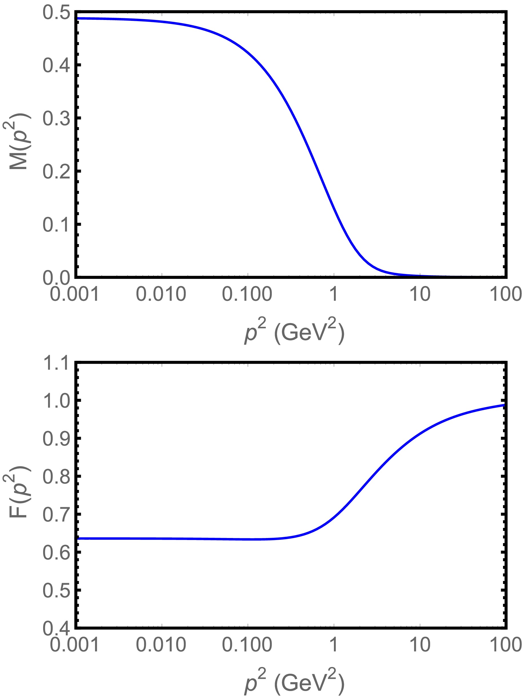
Figure 3. (color online) The quark mass function
$ M(p^2) $ and wave-function renormalization$ F(p^2) $ are shown for the Maris–Tandy (MT) model. These quantities illustrate the model’s general behavior in the chiral limit, in which “gluon-cloud” dressing generates a large constituent-like mass from massless current quarks. This infrared behavior is a prerequisite for describing the observed hadron spectrum.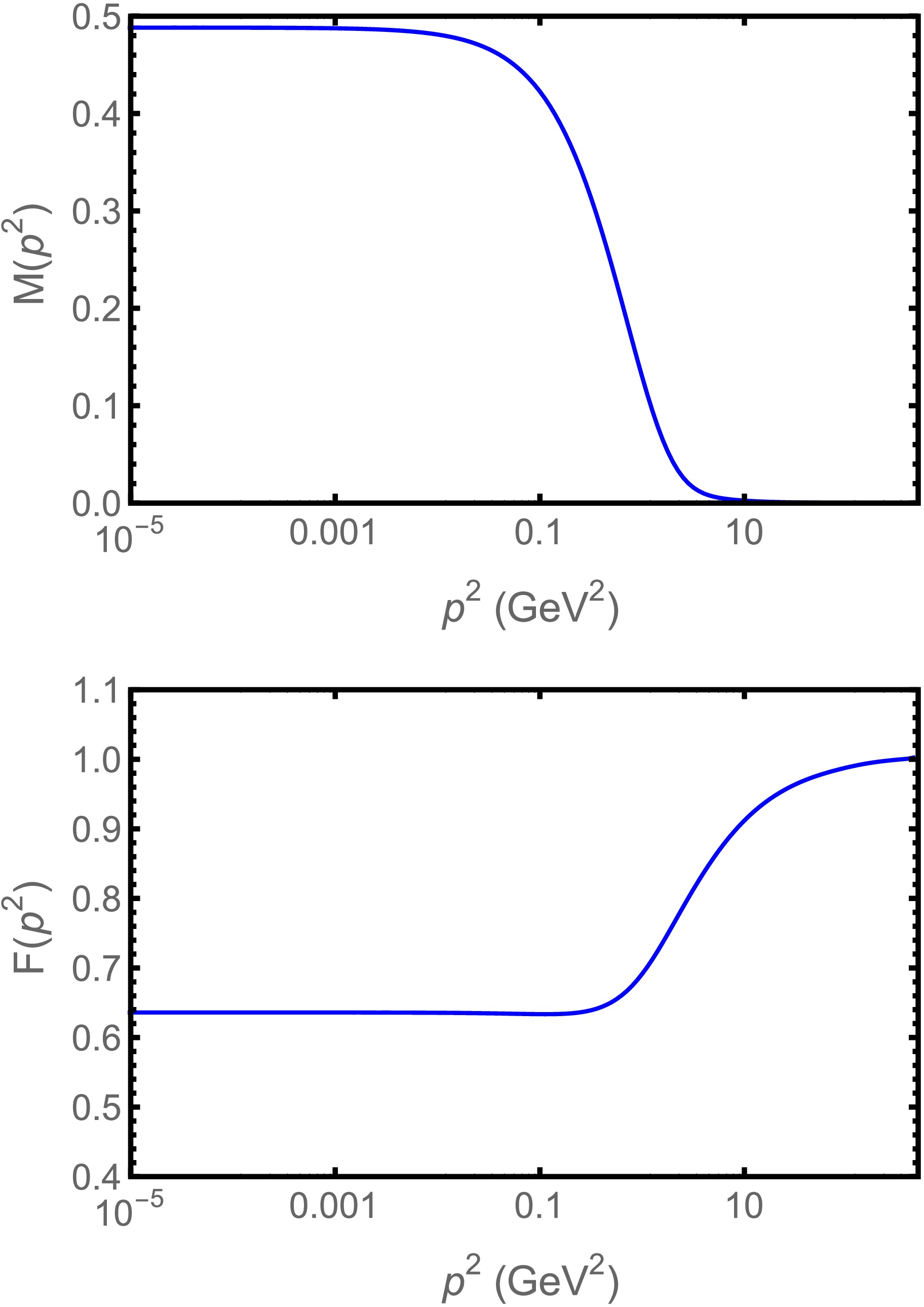
Figure 2. (color online) Behavior of the dressed-quark mass function
$ M(p^2) $ and wave-function renormalization$ F(p^2) $ for the RGZ-model truncation of the SDE in the chiral limit. These plots show that the dressed-quark mass decreases as the momentum increases. In the low-momentum region,$ p^2<1 $ ($ M(0) \approx 0.5 $ GeV), the dressed mass is large because of dynamical chiral symmetry breaking. Conversely, at large momentum,$ p^2>>1 $ , the dressed-quark mass vanishes in the chirally symmetric state. In this limit, the quark wave-function renormalization$ F(p^2) $ approaches unity.3) Lei-Chang et al. [51] proposed a simplified version of the MT model, given by:
$ \frac{4\pi\alpha(q^2)}{q^2} = \frac{4 \pi^2 D q^2 \exp({-\frac{q^2}{\Omega^2}})}{\Omega^6} , $
(30) where
$ \gamma = 12/(33-2N_f) $ ,$ N_f = 4 $ ,$ \tau = e^2 -1 $ ,$ D = 0.93 $ GeV2,$ \Omega = 0.4 $ GeV, and$ D(q^2) = G(q^2)/(q^2) $ . This parametrization provides the most up-to-date and best-performing proposal for predicting hadron spectra within the SDE formalism. Solving the SDE with the above gap equation and the Lei–Cheng model yields the mass function and quark wave-function renormalization shown in Fig. 4. This solution was obtained in the chiral limit in the Landau gauge.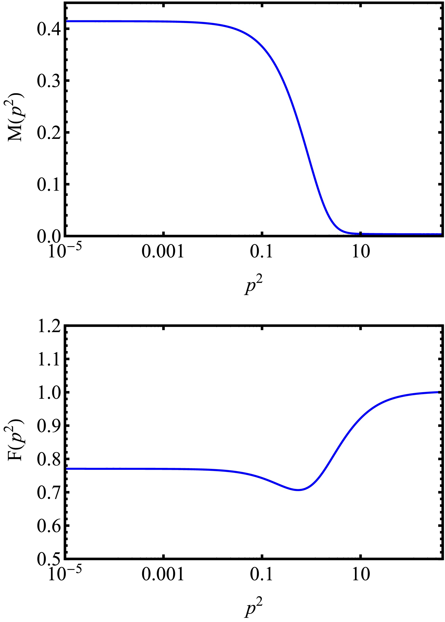
Figure 4. (color online) Mass function
$ M(p^2) $ and wavefunction renormalization$ F(p^2) $ for the Lei–Chang model. This figure shows that, even with a simplified interaction kernel, the SDE framework consistently yields the non-perturbative mass enhancement required to account for the majority of visible mass in the universe through hadronization.More recent attempts to fully describe dynamical mass generation, including for heavy quarks, have considered the Gaussian term in the Lei-Chang model, Eq. (31), complemented by an ansatz for the dressed quark-gluon vertex of the form [51]
$ \Gamma_\mu(k, p) = {\Gamma^{\rm BC}_\mu}(k, p)+{\Gamma^{\rm acm}_\mu}(k, p)\;, $
(31) where
$ {\Gamma^{\rm BC}_\mu}(k, p) = {\rm i}\Sigma_{A}(k^2, p^2)\gamma_\mu+ 2 l_\mu \left[ {\rm i}\gamma\cdot l \Delta_{A}(k^2, p^2)+\Delta_{B}(k^2, p^2) \right] $
(32) is the Ball–Chiu vertex [52], which is constructed to satisfy the Ward–Takahashi identity. The notation used here is
$ \begin{split} \Sigma_{\phi}(p^2_f, p^2_i) &= \frac{1}{2}\left[\phi (p_{f}^2)+ \phi(p_{i}^2) \right]\;,\\ \Delta_{\phi}(p^2_f, p^2_i)& = \frac{1}{\left(p^2_f- p^2_i \right)}\left[ \phi(p_{f}^2)- \phi(p_{i}^2) \right]\;, \end{split} $
(33) and
$ l = (k+p)/2 $ . The transverse vertex accounts for the fact that, if quarks dynamically acquire substantial masses, they should also possess an anomalous chromomagnetic moment$ \Gamma^{\rm acm}_{\mu}(k, p) = {\Gamma^{\rm acm_4}_\mu}(k, p)+{\Gamma^{\rm acm_5}_\mu}(k, p)\;, $
(34) with
$ \Gamma^{\rm acm_4}_{\mu}(k, p) = \left[ l^{T}_{\mu} \gamma\cdot q+ {\rm i}\gamma^{T}_{\mu}\sigma_{\nu\rho}l_{\nu}q_{\rho}\right] \tau_{4} (k, p) \;, $
(35) where the coefficient
$ \tau_{4} (k, p) = {\cal{F}}(z) \left[ \frac{1-2\eta}{M_E} \Delta_{B}(k^2, p^2) -\Delta_{A}(k^2, p^2)\right] $
(36) is defined as
$ {\cal{F}}(z) = (1-e^{-z})/z, $ where$ z = (k^2+ p^2 - 2M^{2}_{E})/ \Lambda^{2}_{{\cal{F}}} $ ,$ \Lambda_{{\cal{F}}} = 1 $ , and$ M_E $ denotes the Euclidean constituent quark mass. Furthermore,$ \Gamma^{\rm acm_5}_{\mu}(k, p) = \sigma_{\mu\nu}q_{\nu} \tau_{5} (k, p,q) \;, $
(37) with
$ \tau_{5} (k, p,q) = \eta \Delta_{B}(k^2, p^2)\;. $
(38) 4) Qin-Chang version of the MT model: Qin and Chang [53] proposed an alternative approximation to the MT model that differs from the Maris–Tandy model because it saturates in the infrared rather than dropping to zero. By contrast, the MT model produces a kernel for the gap equation that has a zero at a small timelike value of
$ q^2 $ and rapidly becomes large and negative as the magnitude of the timelike momentum increases. The Qin-Chang version of the MT model is more consistent with current results from lattice QCD simulations and is given by:$ \begin{split} \dfrac{4\pi\alpha(q^2)}{q^2} :=\;& {4\pi\alpha}\ D(q^2)\equiv \dfrac{8 \pi^2 D \exp({-\dfrac{q^2}{\Omega^2}})}{\Omega^4} \\&+ \dfrac{8\pi^2\gamma_m \left(1-\exp\{-\dfrac{q^2}{4m^2_t}\}\right)}{{q^2}\log\left(\tau+{(1+{(\dfrac{q^2}{\lambda^2}}))}^2\right)}. \end{split} $
(39) The mass and quark wavefunction renormalization plots obtained using this approximation are shown in Fig. 5.
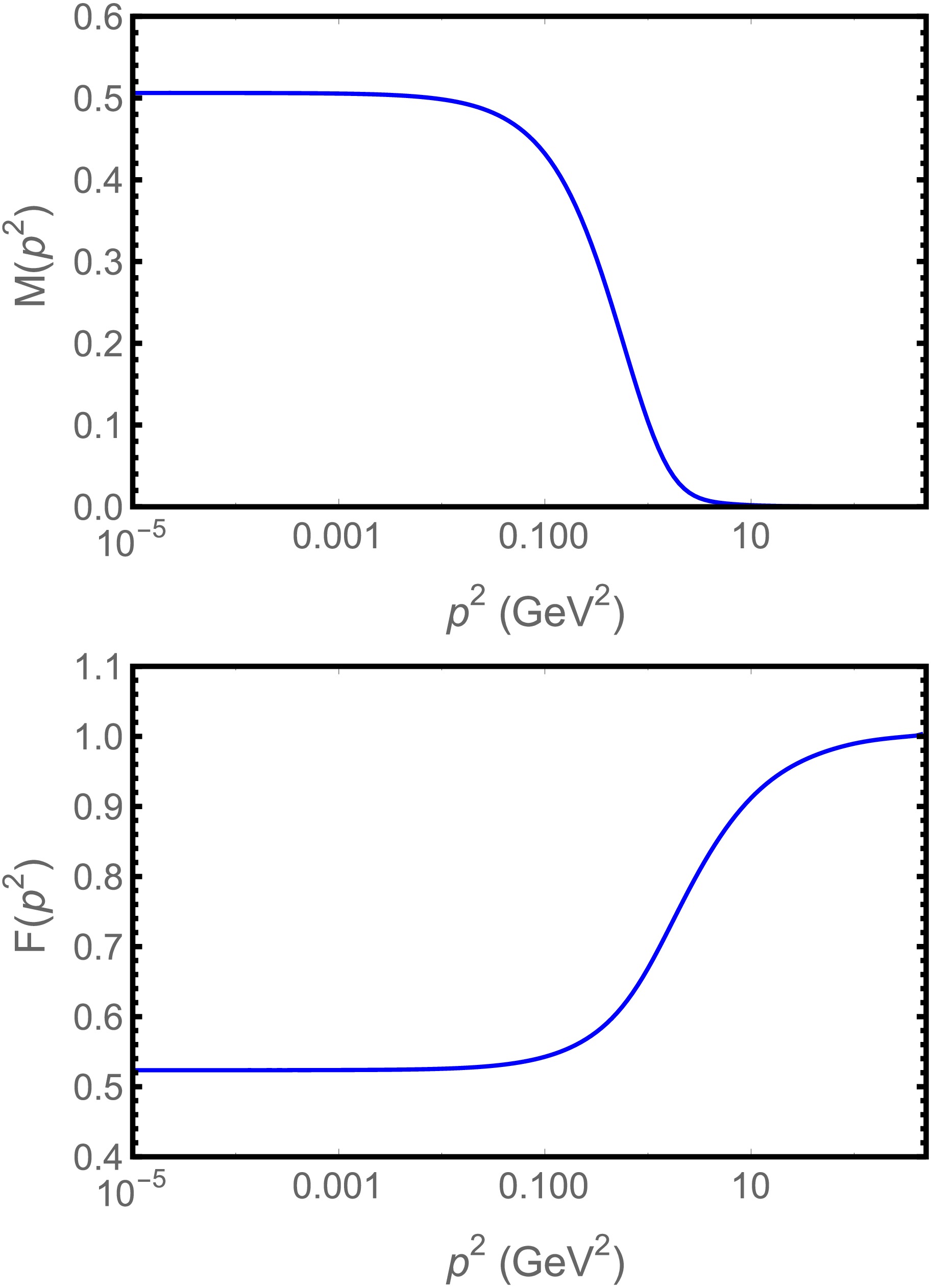
Figure 5. (color online) The mass function
$ M(p^2) $ and wavefunction renormalization$ F(p^2) $ are shown for the Qin–Chang version of the MT model. This comparison highlights how different infrared saturation profiles affect the propagator. The stability of the infrared mass scale across models suggests that dynamical mass generation is a robust emergent feature of QCD, independent of specific truncation details.The above proposal and several other proposals [54] are currently of interest.
5) Contact Interaction Model: Another successful truncation of the Schwinger-Dyson equation is based on a momentum-independent gluon propagator together with the bare-vertex approximation. This approach also describes confinement properties and provides an alternative to the momentum-independent NJL model [20], which does not account for confinement. In the CI, this confinement feature can alternatively be introduced by eliminating the appearance of poles in the quark propagator [34]. This contact interaction model has been effective in studying the static properties of low-energy mesons and baryons. It also preserves the axial-vector Ward–Takahashi identity when the solution to the gap equation is used in the Bethe-Salpeter equation. The model has been extended to finite temperature and density and to the presence of background fields [30, 37−44, 55]. From the perspective of SDE, this model can be seen as a representation in which quarks interact through a contact interaction [34] rather than through massless vector-boson exchange:
$ g^2 D_{\mu \nu}(q^2) = \delta_{\mu \nu} \frac{4 \pi \alpha_{\rm{IR}}}{m_G^2} \equiv \delta_{\mu \nu} \alpha_{\rm{eff}}, $
(40) where
$ \alpha_{\rm{IR}} = 0.93\pi $ represents the infrared-enhanced interaction strength, consistent with current estimates of the zero-momentum value of the running coupling in QCD [56−59]. The gluon mass scale$ m_G = 800 $ MeV is typically associated with the one-loop renormalization-group-improved interaction presented in [53, 60].The model is supplemented by the rainbow-ladder assumption for the vertex,
$ \Gamma_\nu (k,p) = \gamma_\nu $ , which yields a trivial wave-function renormalization,$ A(p^2) = 1 $ , and a momentum-independent quark mass function,$ B(p^2) = M(p^2) = M $ . After performing the angular integration, M is determined self-consistently from$ M = m_{0}+\frac{ \alpha_{\rm{eff}} M }{3\pi^2}\int^{\infty }_{0} {\rm d} s\frac{s}{s+M^2} \,. $
(41) The novel regularization is as follows: first, we exponentiate the denominator of the integrand and then regularize it using the confining proper-time regularization [35]
$ \begin{split} \frac{1}{s+M^2} =\;& \int^{\infty }_{0} {\rm d}\tau {\rm{e}}^{-\tau(s+M^2)}\rightarrow \int^{\tau_{ir}^2}_{\tau_{uv}^2} {\rm d}\tau {\rm{e}}^{-\tau(s+M^2)}\\ =& \frac{ {\rm{e}}^{-\tau^{2}_{uv}(s+M^2)}-{\rm{e}}^{-\tau^{2}_{ir}(s+M^2)}}{s+M^2} \,. \end{split} $
(42) The infrared cutoff, denoted by
$ \tau^{-1}_{ir,uv} = \Lambda_{ir} $ , corresponds to the confinement scale, whereas$ \tau^{-1}_{ir,uv} = \Lambda_{uv} $ represents an ultraviolet dynamical cutoff introduced because the model is nonrenormalizable. This procedure ensures that the quark propagator has no real or complex poles. Such a poleless structure is consistent with quark confinement [35], because an excitation described by a poleless propagator cannot reach its mass shell. The final form of the gap equation is then expressed as:$ M = m_0 + \frac{M^3 \alpha_{\rm{eff}}}{3\pi^2} \left[\Gamma(-1,M^2\tau_{uv}^2)-\Gamma(-1,M^2\tau_{ir}^2)\right] \, , $
(43) where
$ \Gamma(\alpha,x) = \int_x^{\infty} t^{\alpha-1} {\rm{e}}^{-t} {\rm d}t, $
(44) is the incomplete gamma function. In Ref. [61], the parameters
$\alpha_{\rm{eff}} = 5.739\times 10^{-5}\; \mathrm{MeV}^{-2}\; ,$ $ \tau_{ir} = (240\; \mathrm{MeV})^{-1}, $ and$ \tau_{uv} = (905\; \mathrm{MeV})^{-1}\; $ were fitted to study the properties of pions and rho mesons. With the ingredients discussed so far, we can now discuss parameters associated with confinement.The flavor-dependent contact interaction (FCI) model was proposed in [41] to investigate chiral symmetry breaking and restoration for large
$ N_f $ . Ref. [41] introduced a modification to the effective coupling$ \alpha_{\rm{eff}} $ , which enables solutions of the gap equation for larger numbers of flavors. Consequently, the critical number of flavors,$ N^{c}_{f} $ , associated with chiral symmetry breaking and confinement can be determined. The coupling in the FCI model is given by:$ \alpha_{\rm{eff}}(N_f) = \alpha_{\rm{eff}}\sqrt{1 - \frac{(N_{f}-2)}{{\cal{N}}_{f}^{c}}} \,. $
(45) $ \alpha_{\rm{eff}}(N_f) $ denotes the flavor-dressed effective coupling for the contact interaction. For a fixed$ N_f = 2 $ , the effective coupling of the four-fermion contact interaction,$ \alpha_{\rm{eff}}(N_f) $ , reduces to the CI effective coupling$ \alpha_{\rm{eff}} $ . The term$ {\cal{N}}^{c}_{f} = N^{c}_{f} + \varsigma $ in Eq. (45) represents the estimated critical number of flavors, as reported by Ahmad et al. [41, 62]. In this work, with$ \varsigma\approx 2 $ , the chosen parameters yield$ N^{c}_{f} \approx 8 $ , above which dynamical chiral symmetry is restored and deconfinement occurs. The factor$ (N_f-2) $ arises from the fitted parameter ς and does not reflect a physical flavor count; instead, it encodes the behavior of the dynamical mass in relation to vacuum polarization rather than the actual number of flavors.The effective FCI model in Eq. (45) captures the infrared dynamics of QCD and is based on the premise that, for a small number of light quark flavors
$ N_{f} $ , gluon self-interactions produce an anti-screening effect that overwhelms fermion screening. This leads to a strongly coupled theory in the deep infrared, with dynamical symmetry breaking and confinement. As$ N_{f} $ increases, quark-loop contributions grow, causing the theory to become more weakly coupled and driving dynamical chiral symmetry restoration and deconfinement. In this model, the confinement test is conducted via the flavor-dependent confinement scale [38−44, 63]:$ \tilde{\tau}_{ir}(N_f) = \tau_{ir}\frac{M(2)}{M(N_f)}. $
(46) Here,
$ M(2) $ denotes the dressed mass for$ N_f = 2 $ , whereas$ M(N_f) $ is the generalized,$ N_f $ -dependent dressed mass. In the presence of$ N_f $ ,$ \tilde{\tau}_{ir} $ must vary slightly with$ N_f $ . Consequently, the connection between dynamical chiral symmetry breaking and confinement is encoded in a regulator, denoted$ \tilde{\tau}_{ir} $ , that explicitly depends on$ N_f $ . The confinement length scale, Eq. (46), diverges in the chiral limit when chiral symmetry is restored [63]. This drives deconfinement at and above a critical value$ N_{f}^{c} $ , where production thresholds re-emerge [41, 43, 44, 63], consistent with Eq. (41) and NJL-like behavior. One can therefore anticipate direct effects on the bound-state spectrum: dissolution at large$ N_f $ and confinement at small$ N_f $ , as discussed in detail in [63]. -
For several decades, substantial efforts have been made to bring the SDE framework to a predictive stage that is competitive with other nonperturbative frameworks, such as lattice QCD and effective theories. The dressed gluon propagator can be defined from the gauge sector of the Lagrangian in Eq. (1). At tree level, it is given by
$ {\rm i}D^{ab}_{\mu \nu}(q) = \frac{{\rm i}\delta^{ab}}{q^{2}}\left(\delta_{\mu\nu}-(1-\xi)\frac{q_\mu q_\nu}{q^2}\right) , $
(26) where ξ denotes the gauge parameter. Nonperturbatively,
$ {\rm i}D^{ab}_{\mu \nu}(q) = \frac{{\rm i}\delta^{ab}G(q^2)}{q^{2}}\left(\delta_{\mu\nu}-\frac{q_\mu q_\nu}{q^2}\right) +\xi\frac{q_\mu q_\nu \delta^{ab}}{q^4} . $
(27) The behavior of the gluon dressing function
$ G(q^2) $ is of fundamental interest for understanding aspects of confinement [47].1) Lattice-QCD-Motivated Refined Gribov-Zwanziger (RGZ) Model:
A modern understanding of this propagator, consistent with the RGZ confinement scenario [48] and incorporating explicit flavor dependence in the Landau gauge, is given in Ref. [49]
$ D(q^{2}) = \frac{q^{2} + M_{1}^{2}}{q^4 + q^{2} \left(M_{1}^{2}-\dfrac{13g_{0}^{2} \lt A_{1}^{2}>}{24}\right)+ M_{1}^{2} m_{0}^{2}}. $
(28) For this gluon dressing function, the parameters are as follows:
$ M^{2}_{1} = 4.85 $ $ \rm{GeV}^2 $ , which is associated with the condensate of auxiliary fields introduced to preserve the locality of the RGZ action.$ g^{2}_{0}< A_{1}^{2}> = 0.474(16.406-N_{f}) $ $ \rm{GeV}^2 $ is related to the dimension-two gluon condensate, and$ m^2_0 = 1.011(9.161-N_f)^{-1/2} $ $ \rm{GeV}^2 $ . The quark mass function and wave-function renormalization obtained using Eq. (28) are shown in Fig. 22) Maris-Tandy Model: The modern era of SDE studies in hadron physics began with the well-known Maris–Tandy model (MT), which is based on replacing the full quark–gluon vertex and gluon propagator with their bare counterparts, together with a model kernel of the following form [50]
$ \begin{split} \dfrac{4\pi\alpha(q^2)}{q^2} : = {4\pi\alpha}\ D(q^2) \equiv \dfrac{4 \pi^2 D q^2 \exp({-\dfrac{q^2}{\Omega^2}})}{\Omega^6} \end{split} $
$ \begin{split} + \dfrac{8\pi^2\gamma_m \left(1-\exp\{-\dfrac{q^2}{4m^2_t}\}\right)}{{q^2}\log\left(\tau+{(1+{(\dfrac{q^2}{\lambda^2}}))}^2\right)}, \end{split} $
(29) where
$ m_t = 0.5\; {\rm{GeV}} $ ;$ \lambda = 0.234 $ GeV;$ \gamma_{m} = 12/(33-2N_f) $ ;$ N_f = 4 $ ;$ \tau = e^2 -1 $ ;$ D = 0.93 $ GeV2;$ \Omega = 0.4 $ GeV; and$ D(q^2) = G(q^2)/(q^2) $ . The solution of the SDE with the above gap-equation kernel yields$ M(p^2) $ and$ F(p^2) $ , as shown in Fig. 3. This solution was obtained in the chiral limit for light quarks in Landau gauge. The rapid generation of mass for low-momentum quarks, indicated by the large value of the mass function in the infrared momentum domain, is due to the gluon cloud that dresses the quarks.
Figure 3. (color online) The quark mass function
$ M(p^2) $ and wave-function renormalization$ F(p^2) $ are shown for the Maris–Tandy (MT) model. These quantities illustrate the model’s general behavior in the chiral limit, in which “gluon-cloud” dressing generates a large constituent-like mass from massless current quarks. This infrared behavior is a prerequisite for describing the observed hadron spectrum.
Figure 2. (color online) Behavior of the dressed-quark mass function
$ M(p^2) $ and wave-function renormalization$ F(p^2) $ for the RGZ-model truncation of the SDE in the chiral limit. These plots show that the dressed-quark mass decreases as the momentum increases. In the low-momentum region,$ p^2<1 $ ($ M(0) \approx 0.5 $ GeV), the dressed mass is large because of dynamical chiral symmetry breaking. Conversely, at large momentum,$ p^2>>1 $ , the dressed-quark mass vanishes in the chirally symmetric state. In this limit, the quark wave-function renormalization$ F(p^2) $ approaches unity.3) Lei-Chang et al. [51] proposed a simplified version of the MT model, given by:
$ \frac{4\pi\alpha(q^2)}{q^2} = \frac{4 \pi^2 D q^2 \exp({-\frac{q^2}{\Omega^2}})}{\Omega^6} , $
(30) where
$ \gamma = 12/(33-2N_f) $ ,$ N_f = 4 $ ,$ \tau = e^2 -1 $ ,$ D = 0.93 $ GeV2,$ \Omega = 0.4 $ GeV, and$ D(q^2) = G(q^2)/(q^2) $ . This parametrization provides the most up-to-date and best-performing proposal for predicting hadron spectra within the SDE formalism. Solving the SDE with the above gap equation and the Lei–Cheng model yields the mass function and quark wave-function renormalization shown in Fig. 4. This solution was obtained in the chiral limit in the Landau gauge.
Figure 4. (color online) Mass function
$ M(p^2) $ and wavefunction renormalization$ F(p^2) $ for the Lei–Chang model. This figure shows that, even with a simplified interaction kernel, the SDE framework consistently yields the non-perturbative mass enhancement required to account for the majority of visible mass in the universe through hadronization.More recent attempts to fully describe dynamical mass generation, including for heavy quarks, have considered the Gaussian term in the Lei-Chang model, Eq. (31), complemented by an ansatz for the dressed quark-gluon vertex of the form [51]
$ \Gamma_\mu(k, p) = {\Gamma^{\rm BC}_\mu}(k, p)+{\Gamma^{\rm acm}_\mu}(k, p)\;, $
(31) where
$ {\Gamma^{\rm BC}_\mu}(k, p) = {\rm i}\Sigma_{A}(k^2, p^2)\gamma_\mu+ 2 l_\mu \left[ {\rm i}\gamma\cdot l \Delta_{A}(k^2, p^2)+\Delta_{B}(k^2, p^2) \right] $
(32) is the Ball–Chiu vertex [52], which is constructed to satisfy the Ward–Takahashi identity. The notation used here is
$ \begin{split} \Sigma_{\phi}(p^2_f, p^2_i) &= \frac{1}{2}\left[\phi (p_{f}^2)+ \phi(p_{i}^2) \right]\;,\\ \Delta_{\phi}(p^2_f, p^2_i)& = \frac{1}{\left(p^2_f- p^2_i \right)}\left[ \phi(p_{f}^2)- \phi(p_{i}^2) \right]\;, \end{split} $
(33) and
$ l = (k+p)/2 $ . The transverse vertex accounts for the fact that, if quarks dynamically acquire substantial masses, they should also possess an anomalous chromomagnetic moment$ \Gamma^{\rm acm}_{\mu}(k, p) = {\Gamma^{\rm acm_4}_\mu}(k, p)+{\Gamma^{\rm acm_5}_\mu}(k, p)\;, $
(34) with
$ \Gamma^{\rm acm_4}_{\mu}(k, p) = \left[ l^{T}_{\mu} \gamma\cdot q+ {\rm i}\gamma^{T}_{\mu}\sigma_{\nu\rho}l_{\nu}q_{\rho}\right] \tau_{4} (k, p) \;, $
(35) where the coefficient
$ \tau_{4} (k, p) = {\cal{F}}(z) \left[ \frac{1-2\eta}{M_E} \Delta_{B}(k^2, p^2) -\Delta_{A}(k^2, p^2)\right] $
(36) is defined as
$ {\cal{F}}(z) = (1-e^{-z})/z, $ where$ z = (k^2+ p^2 - 2M^{2}_{E})/ \Lambda^{2}_{{\cal{F}}} $ ,$ \Lambda_{{\cal{F}}} = 1 $ , and$ M_E $ denotes the Euclidean constituent quark mass. Furthermore,$ \Gamma^{\rm acm_5}_{\mu}(k, p) = \sigma_{\mu\nu}q_{\nu} \tau_{5} (k, p,q) \;, $
(37) with
$ \tau_{5} (k, p,q) = \eta \Delta_{B}(k^2, p^2)\;. $
(38) 4) Qin-Chang version of the MT model: Qin and Chang [53] proposed an alternative approximation to the MT model that differs from the Maris–Tandy model because it saturates in the infrared rather than dropping to zero. By contrast, the MT model produces a kernel for the gap equation that has a zero at a small timelike value of
$ q^2 $ and rapidly becomes large and negative as the magnitude of the timelike momentum increases. The Qin-Chang version of the MT model is more consistent with current results from lattice QCD simulations and is given by:$ \begin{split} \dfrac{4\pi\alpha(q^2)}{q^2} :=\;& {4\pi\alpha}\ D(q^2)\equiv \dfrac{8 \pi^2 D \exp({-\dfrac{q^2}{\Omega^2}})}{\Omega^4} \\&+ \dfrac{8\pi^2\gamma_m \left(1-\exp\{-\dfrac{q^2}{4m^2_t}\}\right)}{{q^2}\log\left(\tau+{(1+{(\dfrac{q^2}{\lambda^2}}))}^2\right)}. \end{split} $
(39) The mass and quark wavefunction renormalization plots obtained using this approximation are shown in Fig. 5.
Figure 5. (color online) The mass function
$ M(p^2) $ and wavefunction renormalization$ F(p^2) $ are shown for the Qin–Chang version of the MT model. This comparison highlights how different infrared saturation profiles affect the propagator. The stability of the infrared mass scale across models suggests that dynamical mass generation is a robust emergent feature of QCD, independent of specific truncation details.The above proposal and several other proposals [54] are currently of interest.
5) Contact Interaction Model: Another successful truncation of the Schwinger-Dyson equation is based on a momentum-independent gluon propagator together with the bare-vertex approximation. This approach also describes confinement properties and provides an alternative to the momentum-independent NJL model [20], which does not account for confinement. In the CI, this confinement feature can alternatively be introduced by eliminating the appearance of poles in the quark propagator [34]. This contact interaction model has been effective in studying the static properties of low-energy mesons and baryons. It also preserves the axial-vector Ward–Takahashi identity when the solution to the gap equation is used in the Bethe-Salpeter equation. The model has been extended to finite temperature and density and to the presence of background fields [30, 37−44, 55]. From the perspective of SDE, this model can be seen as a representation in which quarks interact through a contact interaction [34] rather than through massless vector-boson exchange:
$ g^2 D_{\mu \nu}(q^2) = \delta_{\mu \nu} \frac{4 \pi \alpha_{\rm{IR}}}{m_G^2} \equiv \delta_{\mu \nu} \alpha_{\rm{eff}}, $
(40) where
$ \alpha_{\rm{IR}} = 0.93\pi $ represents the infrared-enhanced interaction strength, consistent with current estimates of the zero-momentum value of the running coupling in QCD [56−59]. The gluon mass scale$ m_G = 800 $ MeV is typically associated with the one-loop renormalization-group-improved interaction presented in [53, 60].The model is supplemented by the rainbow-ladder assumption for the vertex,
$ \Gamma_\nu (k,p) = \gamma_\nu $ , which yields a trivial wave-function renormalization,$ A(p^2) = 1 $ , and a momentum-independent quark mass function,$ B(p^2) = M(p^2) = M $ . After performing the angular integration, M is determined self-consistently from$ M = m_{0}+\frac{ \alpha_{\rm{eff}} M }{3\pi^2}\int^{\infty }_{0} {\rm d} s\frac{s}{s+M^2} \,. $
(41) The novel regularization is as follows: first, we exponentiate the denominator of the integrand and then regularize it using the confining proper-time regularization [35]
$ \begin{split} \frac{1}{s+M^2} =\;& \int^{\infty }_{0} {\rm d}\tau {\rm{e}}^{-\tau(s+M^2)}\rightarrow \int^{\tau_{ir}^2}_{\tau_{uv}^2} {\rm d}\tau {\rm{e}}^{-\tau(s+M^2)}\\ =& \frac{ {\rm{e}}^{-\tau^{2}_{uv}(s+M^2)}-{\rm{e}}^{-\tau^{2}_{ir}(s+M^2)}}{s+M^2} \,. \end{split} $
(42) The infrared cutoff, denoted by
$ \tau^{-1}_{ir,uv} = \Lambda_{ir} $ , corresponds to the confinement scale, whereas$ \tau^{-1}_{ir,uv} = \Lambda_{uv} $ represents an ultraviolet dynamical cutoff introduced because the model is nonrenormalizable. This procedure ensures that the quark propagator has no real or complex poles. Such a poleless structure is consistent with quark confinement [35], because an excitation described by a poleless propagator cannot reach its mass shell. The final form of the gap equation is then expressed as:$ M = m_0 + \frac{M^3 \alpha_{\rm{eff}}}{3\pi^2} \left[\Gamma(-1,M^2\tau_{uv}^2)-\Gamma(-1,M^2\tau_{ir}^2)\right] \, , $
(43) where
$ \Gamma(\alpha,x) = \int_x^{\infty} t^{\alpha-1} {\rm{e}}^{-t} {\rm d}t, $
(44) is the incomplete gamma function. In Ref. [61], the parameters
$\alpha_{\rm{eff}} = 5.739\times 10^{-5}\; \mathrm{MeV}^{-2}\; ,$ $ \tau_{ir} = (240\; \mathrm{MeV})^{-1}, $ and$ \tau_{uv} = (905\; \mathrm{MeV})^{-1}\; $ were fitted to study the properties of pions and rho mesons. With the ingredients discussed so far, we can now discuss parameters associated with confinement.The flavor-dependent contact interaction (FCI) model was proposed in [41] to investigate chiral symmetry breaking and restoration for large
$ N_f $ . Ref. [41] introduced a modification to the effective coupling$ \alpha_{\rm{eff}} $ , which enables solutions of the gap equation for larger numbers of flavors. Consequently, the critical number of flavors,$ N^{c}_{f} $ , associated with chiral symmetry breaking and confinement can be determined. The coupling in the FCI model is given by:$ \alpha_{\rm{eff}}(N_f) = \alpha_{\rm{eff}}\sqrt{1 - \frac{(N_{f}-2)}{{\cal{N}}_{f}^{c}}} \,. $
(45) $ \alpha_{\rm{eff}}(N_f) $ denotes the flavor-dressed effective coupling for the contact interaction. For a fixed$ N_f = 2 $ , the effective coupling of the four-fermion contact interaction,$ \alpha_{\rm{eff}}(N_f) $ , reduces to the CI effective coupling$ \alpha_{\rm{eff}} $ . The term$ {\cal{N}}^{c}_{f} = N^{c}_{f} + \varsigma $ in Eq. (45) represents the estimated critical number of flavors, as reported by Ahmad et al. [41, 62]. In this work, with$ \varsigma\approx 2 $ , the chosen parameters yield$ N^{c}_{f} \approx 8 $ , above which dynamical chiral symmetry is restored and deconfinement occurs. The factor$ (N_f-2) $ arises from the fitted parameter ς and does not reflect a physical flavor count; instead, it encodes the behavior of the dynamical mass in relation to vacuum polarization rather than the actual number of flavors.The effective FCI model in Eq. (45) captures the infrared dynamics of QCD and is based on the premise that, for a small number of light quark flavors
$ N_{f} $ , gluon self-interactions produce an anti-screening effect that overwhelms fermion screening. This leads to a strongly coupled theory in the deep infrared, with dynamical symmetry breaking and confinement. As$ N_{f} $ increases, quark-loop contributions grow, causing the theory to become more weakly coupled and driving dynamical chiral symmetry restoration and deconfinement. In this model, the confinement test is conducted via the flavor-dependent confinement scale [38−44, 63]:$ \tilde{\tau}_{ir}(N_f) = \tau_{ir}\frac{M(2)}{M(N_f)}. $
(46) Here,
$ M(2) $ denotes the dressed mass for$ N_f = 2 $ , whereas$ M(N_f) $ is the generalized,$ N_f $ -dependent dressed mass. In the presence of$ N_f $ ,$ \tilde{\tau}_{ir} $ must vary slightly with$ N_f $ . Consequently, the connection between dynamical chiral symmetry breaking and confinement is encoded in a regulator, denoted$ \tilde{\tau}_{ir} $ , that explicitly depends on$ N_f $ . The confinement length scale, Eq. (46), diverges in the chiral limit when chiral symmetry is restored [63]. This drives deconfinement at and above a critical value$ N_{f}^{c} $ , where production thresholds re-emerge [41, 43, 44, 63], consistent with Eq. (41) and NJL-like behavior. One can therefore anticipate direct effects on the bound-state spectrum: dissolution at large$ N_f $ and confinement at small$ N_f $ , as discussed in detail in [63]. -
The axiom of positivity violation states that ''if a certain degree of freedom has negative-norm contributions in its propagator, it cannot represent a physical asymptotic state, indicating the absence of a Kallen-Lehmann spectral representation for its propagator'' [47]. This concept is crucial in Euclidean quantum field theory, where positivity is formulated through the Osterwalder-Schrader axiom of reflection positivity [64]. In particular, for a two-point correlation function
$ \Delta^{\prime}(x-y) $ , this condition can be expressed as follows:$ \int \ {\rm d}^{4}x \ d^{4}y\; \bar{{\cal{G}}}(\vec{x}, x_{4})\Delta^{\prime}(x-y) {\cal{G}}(\vec{y}, y_{4})\geq0. $
(47) Here,
$ {\cal{G}}(\vec{x}, x_{4}) $ is a complex-valued test function with support in$ \lbrace(\vec{x}, x_{4}):x_{4} = t>0\rbrace $ . Using the three-dimensional Fourier transform, as discussed in [47], we have:$ \int_{0}^{\infty} {\rm d}{t}\int_{0}^{\infty} {\rm d}{t^{\prime}} \int {\rm d}^{3}p\; \bar{\tilde{{\cal{G}}}}(t, \vec{p})\Delta\left( -(t+t^{\prime}), \vec{p}\right) \tilde{{\cal{G}}}(t^{\prime}, \vec{p})\geq0. $
(48) The above-mentioned condition is violated only in a region around
$ t_0 = (t+t^{\prime}) $ where$ \Delta\left( -t_{0}, \vec{p}\right)<0 $ . By considering a real test function$ {\cal{G}}(t) $ with peaks at t and$ t^{\prime} $ , one can immediately observe a violation of reflection positivity. Therefore, in the special case$ \vec{p} = 0 $ , the condition given in Eq. (48) permits the definition of ''spatially averaged Schwinger functions'' from the propagators. In particular, for the gluon propagator, one can define:$ \Delta(\tau) = \frac{1}{2\pi}\int {\rm d} p_{4} {\rm e}^{-{\rm i}p_{4}\tau} G(p_4,\vec{0})\;. $
(49) As shown in Fig. 6, this function is not positive-definite for the RGZ proposal of the gluon propagator in Eq. (28) and is therefore consistent with confinement. The sharp peak in the plot of
$ \log{|\Delta(\tau)|} $ indicates a crossing of$ \Delta(\tau) $ with the horizontal axis. The inverse of the crossing position serves as an order parameter for confinement [65, 66]. This framework admits a clearer interpretation in the fermionic case. We define the spatially averaged function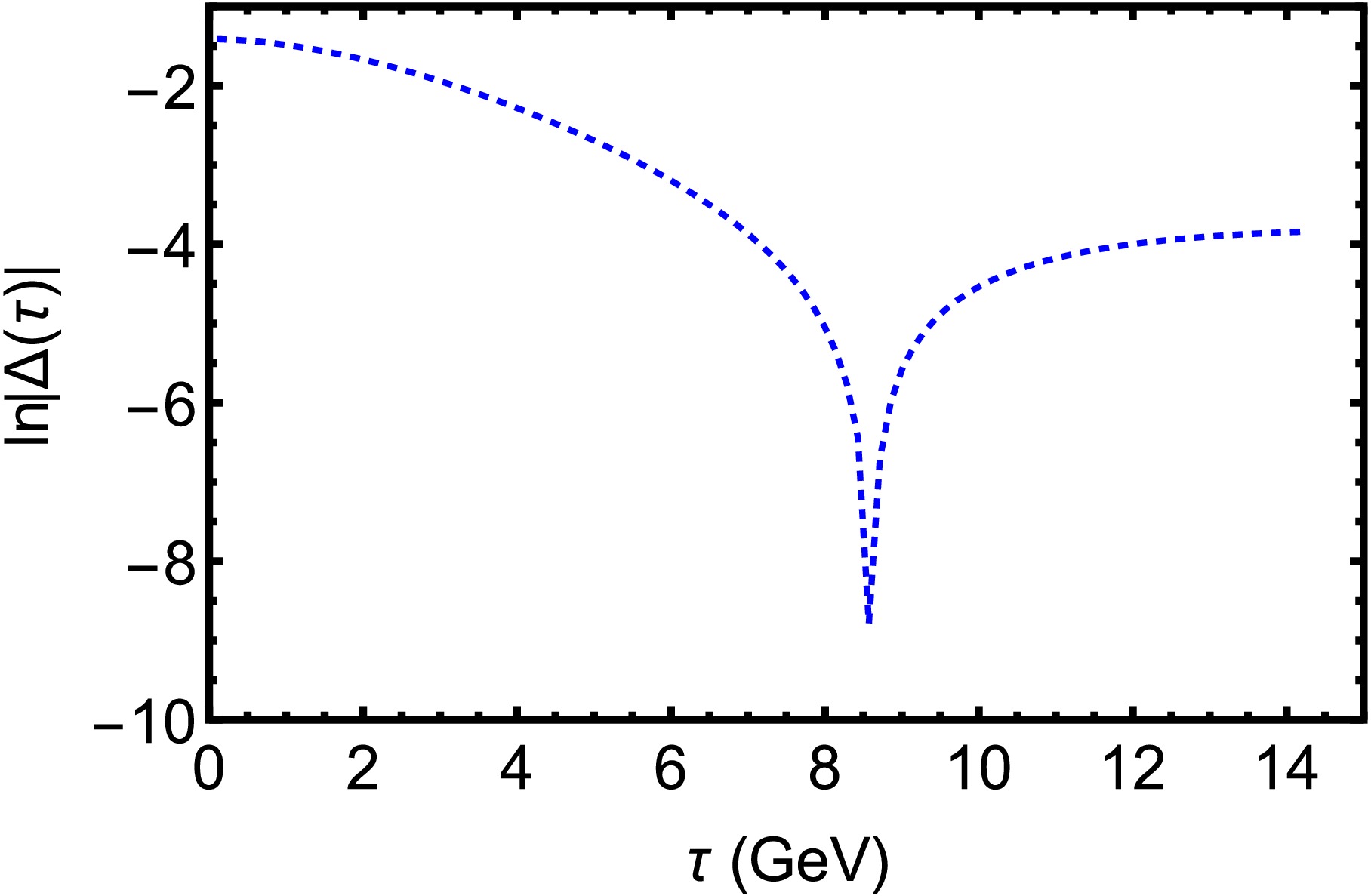
Figure 6. (color online) A confinement test for the RGZ model is performed using the spatially averaged Schwinger function
$ \Delta_s(\tau) $ . Either the "cusp" at$ \tau \approx 8.6 $ GeV−1 (indicated by the dip in the logarithmic plot) or the subsequent crossing into negative values demonstrates a violation of the reflection positivity axiom (i.e., the absence of a Källén–Lehmann representation). This provides mathematical proof that the quark cannot be an asymptotic physical state, thereby confirming its confinement.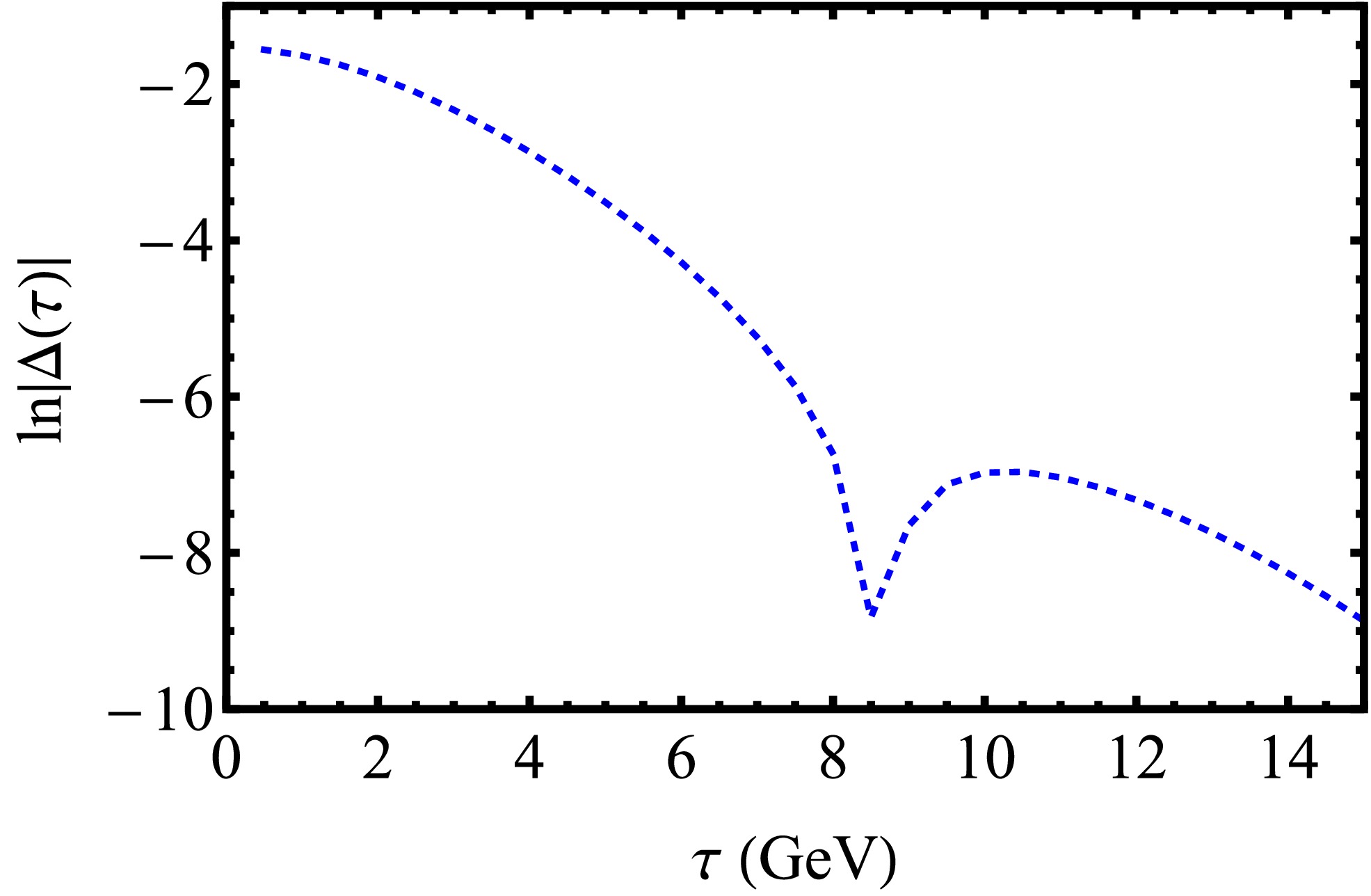
Figure 7. (color online) A confinement test for the MT model is performed using the Schwinger function. The cusp at
$ \tau \approx 8.5 $ GeV−1 indicates the absence of a Kallen–Lehmann representation. This behavior is a definitive signal that the model describes a confining theory in which quarks do not appear in the physical spectrum.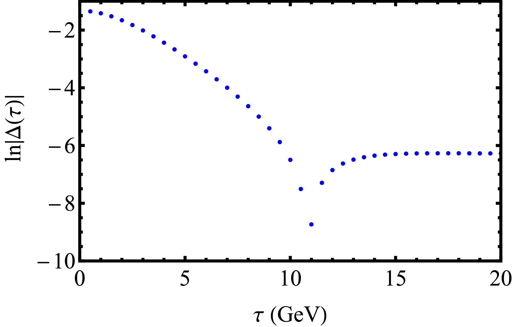
Figure 8. (color online) Confinement test for the Lei–Chang model. Despite its simplified interaction kernel, the cusp at
$ \tau \approx 10.5 $ GeV−1 in the logarithmic Schwinger function confirms that the model captures the essential non-perturbative physics required to enforce quark confinement.$ \begin{split} \Delta_s(\tau) =\;& \frac{1}{2\pi}\int {\rm d} p_{4} {\rm e}^{-{\rm i}p_{4}\tau} \sigma_{s}(p_{4},\vec{0})\\ =\;& \frac{1}{\pi}\int {\rm d} p_{4}{\rm{cos}}(p_{4}\tau)\sigma_{s}(p_{4},\vec{0})\geqslant0. \end{split}$
(50) The large-τ behavior of
$ \Delta_s(\tau) $ determines the type of excitation described by the fermion propagator. For a stable particle,$ \Delta_s(\tau)\geq 0 $ , whereas for a confined particle,$ \Delta_s(\tau) $ changes sign as τ increases [47, 64, 65]. The physical interpretation of the axis crossing in Fig. 6 through Fig. 9 is critical. In a theory with physical (unconfined) particles, the Schwinger function must remain positive to satisfy the Källén–Lehmann representation. The “stiff peak” followed by a transition to negative values in these plots provides mathematical evidence that these degrees of freedom do not appear in the physical spectrum, thereby serving as a definitive signal of confinement within these specific SDE truncations.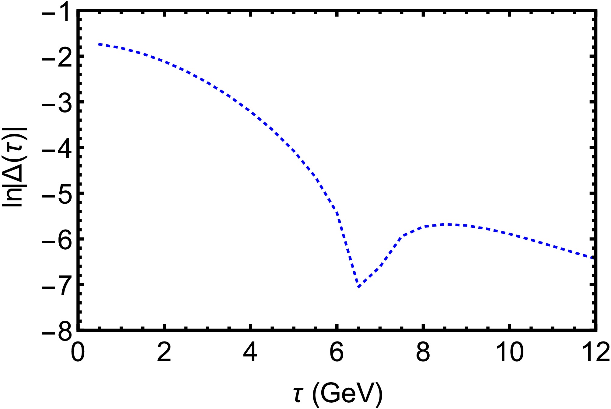
Figure 9. (color online) Confinement test for the Qin–Chang model. Here, the cusp is located at
$ \tau \approx 6.5 $ GeV−1, indicating confinement. The similarity to Figs. 6–8 highlights that the violation of reflection positivity is a universal feature of successful SDE truncations and serves as a reliable and robust proxy for the confinement–deconfinement transition.In quantum field theory, the fermion propagator typically has real poles and pairs of complex conjugate poles. To investigate confinement, we analyze the poles of the propagator in the complex
$ p^{2} $ -plane. Real poles lead to an exponentially decaying$ \Delta_{s}(\tau) $ given by:$ \Delta_s(\tau)\sim {\rm e}^{-M\tau}, $
(51) indicating a stable asymptotic state. By contrast, complex conjugate pairs of poles give rise to dynamical masses with a nonzero imaginary part,
$ M = {\cal{A}}\pm {\rm i} {\cal{B}} $ , representing short-lived excitations that decay exponentially over large timelike distances$ \Delta_s(\tau)\sim {\rm e}^{-{\cal{A}}\tau} {\rm{cos}}({\cal{B}} \tau+\delta), $
(52) where δ is a phase. The presence of complex-conjugate poles in the propagator naturally leads to a violation of reflection positivity. All truncations considered here are consistent with the axiom of reflection positivity, as shown in Figs. 6–9. The above test cannot be performed in the NJL-type model.
A viewpoint on confinement, distinct from reflection positivity, arises for
$ x = p^2>0 $ ; in this case, the inflection point$ x_c $ , which serves as the confinement order parameter [11], can be defined as:$ \frac{{\rm d}^2\sigma_{v}(x)}{{\rm d}x^2}\Bigg|_{x = x_{c}} = 0, $
(53) provided
$ x_{c}>0 $ . This condition defines the point at which the second derivative of$ \sigma_v(x) $ vanishes, provided that$ x_c $ is positive. The absence of inflection points indicates the absence of confinement in the propagator. Their presence is established when the first derivative${\rm d}\sigma_v/{\rm d}x$ reaches an extremum. Figs. 10–13 show that the derivative of$ \sigma_v(x) $ reaches an extremum for all successful truncations under consideration. This extremum corresponds to the inflection point and serves as an order parameter for confinement. The inflection point$ x_c $ provides a scale that separates the perturbative and non-perturbative regimes. In Figs. 10–13, the extremum in the derivative of the vector projection$ \sigma_v $ is not merely a geometric feature; it represents the momentum scale at which the dressing effects of the gluon cloud are strongest. The absence of such an inflection point in a model would imply a lack of confinement, making this criterion a robust comparative tool across different kernels. A particular form of the spatially averaged propagator for testing confinement with constant masses was considered in Refs. [65, 66]. At finite T, it is given by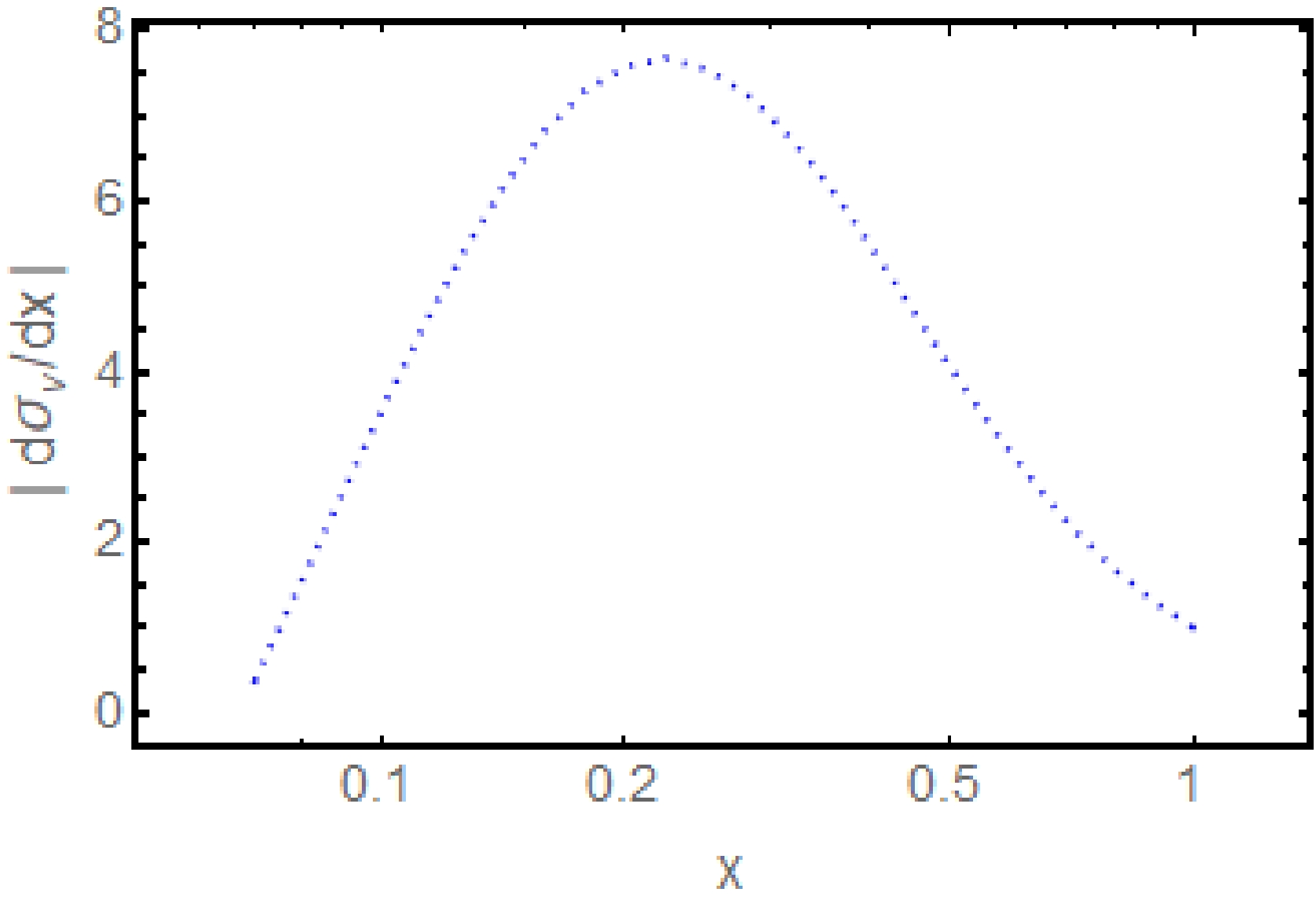
Figure 10. (color online) Derivative of the vector projection of the quark propagator,
$|{\rm d}\sigma_V/{\rm d}x|$ , for the RGZ model. The extremum in this plot, located at$ x \approx 0.3 $ GeV2, identifies the inflection point$ x_c $ , which serves as a quantitative order parameter for confinement. This peak marks the momentum scale at which gluonic dressing effects are strongest.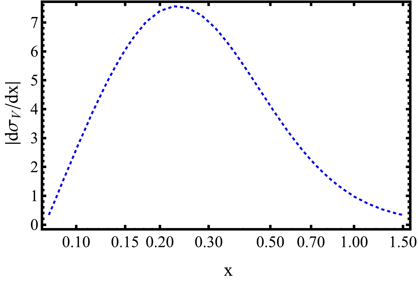
Figure 11. (color online) Inflection-point analysis of the MT model. The sharp peak at
$ x \approx 0.25 $ GeV2 identifies the specific confinement scale associated with this interaction. This diagnostic tool enables a clear distinction between the perturbative (high-x) and nonperturbative (low-x) regimes of the theory.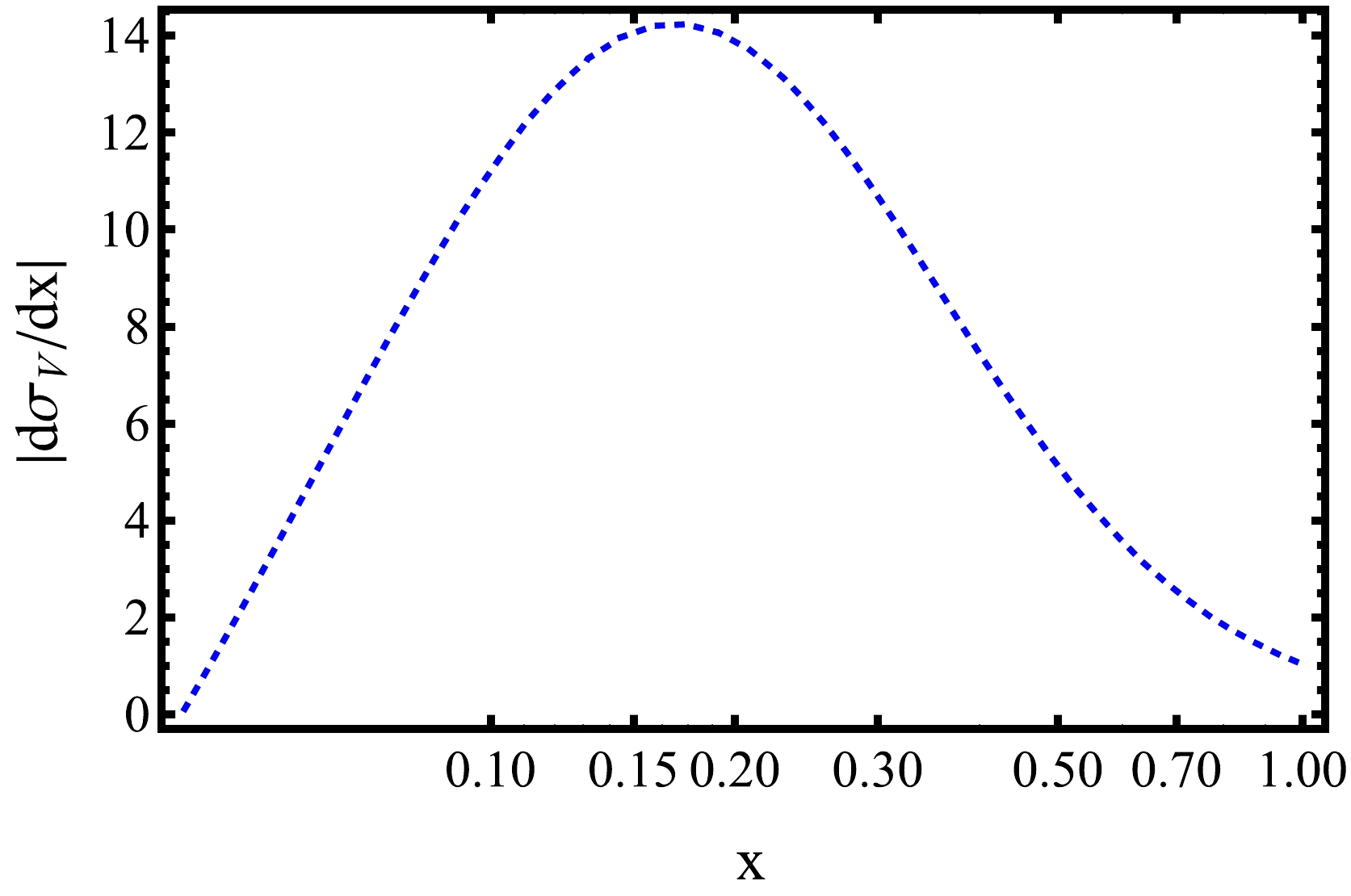
Figure 12. (color online) Inflection-point analysis for the Lei-Chang model. The existence of a well-defined extremum (at
$ x\approx 0.17 $ GeV2) confirms that the simplified model preserves the analytic structure indicative of a confined excitation, thereby supporting its validity for predicting hadron properties.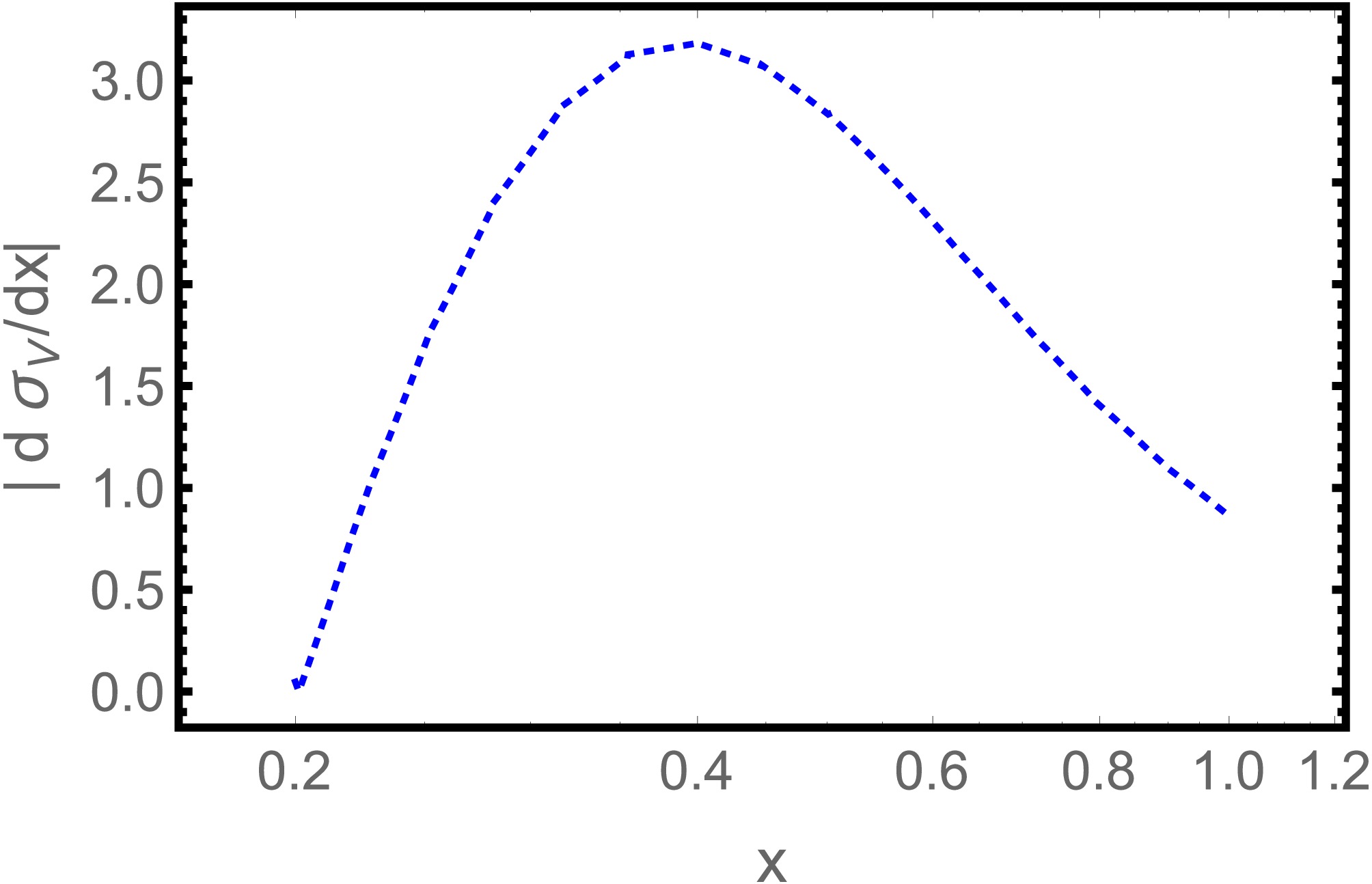
Figure 13. (color online) This analysis examines the inflection point (at
$ x \approx 0.37 $ GeV2) in the Qin–Chang model. Comparing this point with Fig. 11 shows how variations in the infrared kernel shift the confinement scale, providing a means of tuning model parameters using lattice QCD data.$ \Delta(\tau) = T \sum\limits_{n} {\rm e}^{-{\rm i}\tilde{\omega}_{n}\tau} \frac{M(\tilde{\omega}^{2}_{n})}{\tilde{\omega}^{2}_{n}+ M^{2}(\tilde{\omega}^{2}_{n})}. $
(54) Figure 14 illustrates the variation of
$ \Delta(\tau) $ at different temperatures. At low temperatures,$ \Delta(\tau) $ exhibits significant oscillations, indicating confinement. As the temperature increases, the oscillation amplitude decreases until the oscillations disappear at a critical temperature$ T_c $ , signaling the transition to deconfinement [66, 67].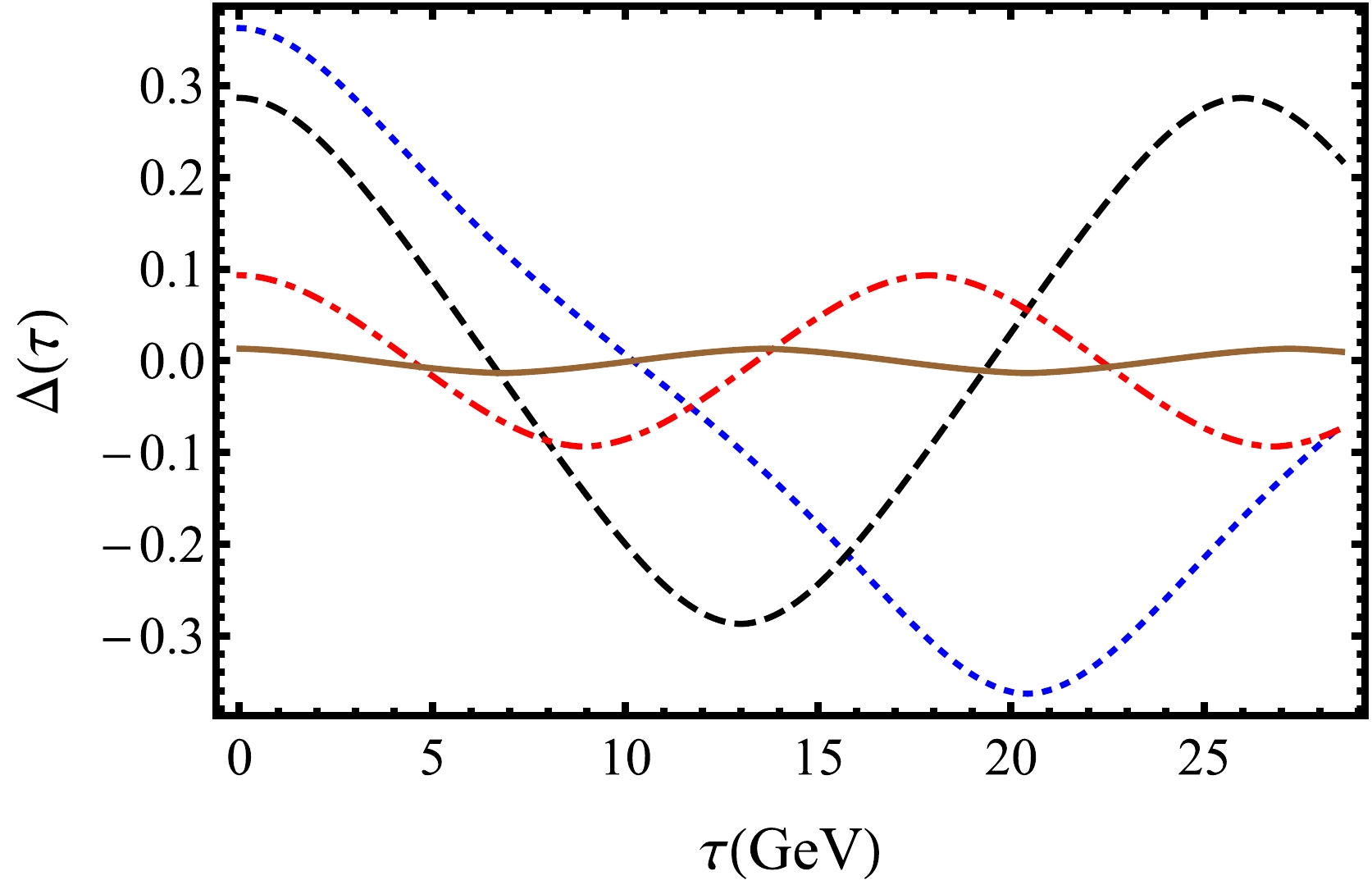
Figure 14. (color online)
$ \Delta(\tau) $ for various T as a function of τ. The blue dotted curve is plotted at$ T = 0.07 $ GeV, the black dashed curve at$ T = 0.11 $ GeV, the red dot-dashed curve at$ T = 0.16 $ GeV, and the solid brown curve at$ T = 0.21 $ GeV. The Schwinger function oscillates, and the mass function has singularities; these features provide an unambiguous signal for the absence of a Lehmann representation and hence for confinement. As the temperature increases, no zero crossing occurs above a critical temperature$ T_c $ , thus indicating deconfinement. -
The axiom of positivity violation states that ''if a certain degree of freedom has negative-norm contributions in its propagator, it cannot represent a physical asymptotic state, indicating the absence of a Kallen-Lehmann spectral representation for its propagator'' [47]. This concept is crucial in Euclidean quantum field theory, where positivity is formulated through the Osterwalder-Schrader axiom of reflection positivity [64]. In particular, for a two-point correlation function
$ \Delta^{\prime}(x-y) $ , this condition can be expressed as follows:$ \int \ {\rm d}^{4}x \ d^{4}y\; \bar{{\cal{G}}}(\vec{x}, x_{4})\Delta^{\prime}(x-y) {\cal{G}}(\vec{y}, y_{4})\geq0. $
(47) Here,
$ {\cal{G}}(\vec{x}, x_{4}) $ is a complex-valued test function with support in$ \lbrace(\vec{x}, x_{4}):x_{4} = t>0\rbrace $ . Using the three-dimensional Fourier transform, as discussed in [47], we have:$ \int_{0}^{\infty} {\rm d}{t}\int_{0}^{\infty} {\rm d}{t^{\prime}} \int {\rm d}^{3}p\; \bar{\tilde{{\cal{G}}}}(t, \vec{p})\Delta\left( -(t+t^{\prime}), \vec{p}\right) \tilde{{\cal{G}}}(t^{\prime}, \vec{p})\geq0. $
(48) The above-mentioned condition is violated only in a region around
$ t_0 = (t+t^{\prime}) $ where$ \Delta\left( -t_{0}, \vec{p}\right)<0 $ . By considering a real test function$ {\cal{G}}(t) $ with peaks at t and$ t^{\prime} $ , one can immediately observe a violation of reflection positivity. Therefore, in the special case$ \vec{p} = 0 $ , the condition given in Eq. (48) permits the definition of ''spatially averaged Schwinger functions'' from the propagators. In particular, for the gluon propagator, one can define:$ \Delta(\tau) = \frac{1}{2\pi}\int {\rm d} p_{4} {\rm e}^{-{\rm i}p_{4}\tau} G(p_4,\vec{0})\;. $
(49) As shown in Fig. 6, this function is not positive-definite for the RGZ proposal of the gluon propagator in Eq. (28) and is therefore consistent with confinement. The sharp peak in the plot of
$ \log{|\Delta(\tau)|} $ indicates a crossing of$ \Delta(\tau) $ with the horizontal axis. The inverse of the crossing position serves as an order parameter for confinement [65, 66]. This framework admits a clearer interpretation in the fermionic case. We define the spatially averaged function
Figure 6. (color online) A confinement test for the RGZ model is performed using the spatially averaged Schwinger function
$ \Delta_s(\tau) $ . Either the "cusp" at$ \tau \approx 8.6 $ GeV−1 (indicated by the dip in the logarithmic plot) or the subsequent crossing into negative values demonstrates a violation of the reflection positivity axiom (i.e., the absence of a Källén–Lehmann representation). This provides mathematical proof that the quark cannot be an asymptotic physical state, thereby confirming its confinement.
Figure 7. (color online) A confinement test for the MT model is performed using the Schwinger function. The cusp at
$ \tau \approx 8.5 $ GeV−1 indicates the absence of a Kallen–Lehmann representation. This behavior is a definitive signal that the model describes a confining theory in which quarks do not appear in the physical spectrum.
Figure 8. (color online) Confinement test for the Lei–Chang model. Despite its simplified interaction kernel, the cusp at
$ \tau \approx 10.5 $ GeV−1 in the logarithmic Schwinger function confirms that the model captures the essential non-perturbative physics required to enforce quark confinement.$ \begin{split} \Delta_s(\tau) =\;& \frac{1}{2\pi}\int {\rm d} p_{4} {\rm e}^{-{\rm i}p_{4}\tau} \sigma_{s}(p_{4},\vec{0})\\ =\;& \frac{1}{\pi}\int {\rm d} p_{4}{\rm{cos}}(p_{4}\tau)\sigma_{s}(p_{4},\vec{0})\geqslant0. \end{split}$
(50) The large-τ behavior of
$ \Delta_s(\tau) $ determines the type of excitation described by the fermion propagator. For a stable particle,$ \Delta_s(\tau)\geq 0 $ , whereas for a confined particle,$ \Delta_s(\tau) $ changes sign as τ increases [47, 64, 65]. The physical interpretation of the axis crossing in Fig. 6 through Fig. 9 is critical. In a theory with physical (unconfined) particles, the Schwinger function must remain positive to satisfy the Källén–Lehmann representation. The “stiff peak” followed by a transition to negative values in these plots provides mathematical evidence that these degrees of freedom do not appear in the physical spectrum, thereby serving as a definitive signal of confinement within these specific SDE truncations.
Figure 9. (color online) Confinement test for the Qin–Chang model. Here, the cusp is located at
$ \tau \approx 6.5 $ GeV−1, indicating confinement. The similarity to Figs. 6–8 highlights that the violation of reflection positivity is a universal feature of successful SDE truncations and serves as a reliable and robust proxy for the confinement–deconfinement transition.In quantum field theory, the fermion propagator typically has real poles and pairs of complex conjugate poles. To investigate confinement, we analyze the poles of the propagator in the complex
$ p^{2} $ -plane. Real poles lead to an exponentially decaying$ \Delta_{s}(\tau) $ given by:$ \Delta_s(\tau)\sim {\rm e}^{-M\tau}, $
(51) indicating a stable asymptotic state. By contrast, complex conjugate pairs of poles give rise to dynamical masses with a nonzero imaginary part,
$ M = {\cal{A}}\pm {\rm i} {\cal{B}} $ , representing short-lived excitations that decay exponentially over large timelike distances$ \Delta_s(\tau)\sim {\rm e}^{-{\cal{A}}\tau} {\rm{cos}}({\cal{B}} \tau+\delta), $
(52) where δ is a phase. The presence of complex-conjugate poles in the propagator naturally leads to a violation of reflection positivity. All truncations considered here are consistent with the axiom of reflection positivity, as shown in Figs. 6–9. The above test cannot be performed in the NJL-type model.
A viewpoint on confinement, distinct from reflection positivity, arises for
$ x = p^2>0 $ ; in this case, the inflection point$ x_c $ , which serves as the confinement order parameter [11], can be defined as:$ \frac{{\rm d}^2\sigma_{v}(x)}{{\rm d}x^2}\Bigg|_{x = x_{c}} = 0, $
(53) provided
$ x_{c}>0 $ . This condition defines the point at which the second derivative of$ \sigma_v(x) $ vanishes, provided that$ x_c $ is positive. The absence of inflection points indicates the absence of confinement in the propagator. Their presence is established when the first derivative${\rm d}\sigma_v/{\rm d}x$ reaches an extremum. Figs. 10–13 show that the derivative of$ \sigma_v(x) $ reaches an extremum for all successful truncations under consideration. This extremum corresponds to the inflection point and serves as an order parameter for confinement. The inflection point$ x_c $ provides a scale that separates the perturbative and non-perturbative regimes. In Figs. 10–13, the extremum in the derivative of the vector projection$ \sigma_v $ is not merely a geometric feature; it represents the momentum scale at which the dressing effects of the gluon cloud are strongest. The absence of such an inflection point in a model would imply a lack of confinement, making this criterion a robust comparative tool across different kernels. A particular form of the spatially averaged propagator for testing confinement with constant masses was considered in Refs. [65, 66]. At finite T, it is given by
Figure 10. (color online) Derivative of the vector projection of the quark propagator,
$|{\rm d}\sigma_V/{\rm d}x|$ , for the RGZ model. The extremum in this plot, located at$ x \approx 0.3 $ GeV2, identifies the inflection point$ x_c $ , which serves as a quantitative order parameter for confinement. This peak marks the momentum scale at which gluonic dressing effects are strongest.
Figure 11. (color online) Inflection-point analysis of the MT model. The sharp peak at
$ x \approx 0.25 $ GeV2 identifies the specific confinement scale associated with this interaction. This diagnostic tool enables a clear distinction between the perturbative (high-x) and nonperturbative (low-x) regimes of the theory.
Figure 12. (color online) Inflection-point analysis for the Lei-Chang model. The existence of a well-defined extremum (at
$ x\approx 0.17 $ GeV2) confirms that the simplified model preserves the analytic structure indicative of a confined excitation, thereby supporting its validity for predicting hadron properties.
Figure 13. (color online) This analysis examines the inflection point (at
$ x \approx 0.37 $ GeV2) in the Qin–Chang model. Comparing this point with Fig. 11 shows how variations in the infrared kernel shift the confinement scale, providing a means of tuning model parameters using lattice QCD data.$ \Delta(\tau) = T \sum\limits_{n} {\rm e}^{-{\rm i}\tilde{\omega}_{n}\tau} \frac{M(\tilde{\omega}^{2}_{n})}{\tilde{\omega}^{2}_{n}+ M^{2}(\tilde{\omega}^{2}_{n})}. $
(54) Figure 14 illustrates the variation of
$ \Delta(\tau) $ at different temperatures. At low temperatures,$ \Delta(\tau) $ exhibits significant oscillations, indicating confinement. As the temperature increases, the oscillation amplitude decreases until the oscillations disappear at a critical temperature$ T_c $ , signaling the transition to deconfinement [66, 67].
Figure 14. (color online)
$ \Delta(\tau) $ for various T as a function of τ. The blue dotted curve is plotted at$ T = 0.07 $ GeV, the black dashed curve at$ T = 0.11 $ GeV, the red dot-dashed curve at$ T = 0.16 $ GeV, and the solid brown curve at$ T = 0.21 $ GeV. The Schwinger function oscillates, and the mass function has singularities; these features provide an unambiguous signal for the absence of a Lehmann representation and hence for confinement. As the temperature increases, no zero crossing occurs above a critical temperature$ T_c $ , thus indicating deconfinement. -
In lattice QCD, the confinement/deconfinement transition is typically studied by examining the behavior of the Polyakov loop (PL)
$ {\cal{P}} $ [16], which is the expectation value of a Wilson loop wrapping around the periodic Euclidean time direction. The Polyakov loop is explicitly defined as:$ {\cal{P}} = \frac{1}{N_{c}}\langle {\rm{Tr}}\left[ \Pi {\rm{e}}^{ {-\int^{1/T}_{0} {\rm d}\tau A_{0}}}\right] \rangle. $
(55) Here, Π represents the path ordering of the exponential, and
$ N_{c} $ is the number of colors. At finite T, the action S in the pure-gauge sector with gauge group$ S U(N_c) $ has a global$ Z(N_c) $ symmetry [68]. This symmetry is spontaneously broken, and the PL expectation value is considered the order parameter. This follows because we can write$ {\cal{P}} $ as:$ {\cal{P}} = {\rm e}^{-E_{q}(T)/T}\;. $
(56) The free energy of a single quark in a gluonic heat bath is denoted by
$ E_{q}(T) $ . In the confined phase, where$ \langle {\cal{P}}\rangle = 0 $ , corresponding to$ E_{q}(T)\rightarrow \infty $ , the quark is confined. In contrast, in the deconfined phase, where$ \langle {\cal{P}}\rangle\neq0 $ ,$ E_{q}(T) $ is finite, indicating that quarks are deconfined.A few years ago, another order parameter, referred to as the ''dual quark condensate'' or dPL, was introduced to explore the confinement–deconfinement phase transition in lattice [24, 25] and continuum SDE studies [27−30]. It has also been explored in variants of the NJL model [69−71] and QED3 [72]. The dPL is commonly denoted by
$ \Sigma_{n} $ and is defined as$ \Sigma_{n} = -\int^{2\pi}_{0}\frac{{\rm d}\phi}{2\pi} {\rm e}^{-{\rm i} n\phi} \langle\bar{\psi}\psi\rangle_{\phi}, $
(57) where n is an integer, and
$ \Sigma_{n} $ is the projection of$ \langle\bar{\psi}\psi\rangle_{\phi} $ onto loops winding n times around the temporal direction. The ϕ-dependent condensate can be obtained from the ϕ-dependent quark propagator as$ \langle \bar{\psi}\psi\rangle_{\phi} = N_{c}T\sum\limits_{n}\int \frac{{\rm d}^3\vec{k}}{(2\pi)^3}{\rm{Tr}}[S(\vec{k},\omega_{n}^{\phi})]. $
(58) The generalized condensate
$ \langle \bar{\psi}\psi\rangle_{\phi} $ is defined as the quark condensate evaluated for quark fields satisfying twisted boundary conditions:$ \psi(1/T,\vec{x}) = {\rm{e}}^{-{\rm i}\phi}\psi(0,\vec{x}), $
(59) in the imaginary-time direction, where
$ \phi\in[0,2\pi] $ . For$ \phi = \pi $ , the standard anti-periodicity of ψ can be retained. The above-mentioned$ U(1) $ -valued boundary conditions in momentum space yield generalized ϕ- dependent Matsubara frequencies,$ \omega_n\rightarrow \omega_{n}^{\phi} = (2n+ \phi/ \pi)\pi T $ , obtained by slightly modifying the usual fermionic Matsubara frequencies through the inclusion of a purely imaginary chemical potential,$ \mu_I = \phi T $ . From the lattice QCD perspective, it can be defined as a sum of Wilson loops winding n times around the temporal boundary [24, 25]. The shortest Pl with winding number$ n = 1 $ , considered as a collection of generalized Pl with spatial fluctuations, is referred to as the ''dressed Polyakov loop (dPl)'' [24, 25]$ \Sigma_1 = -\int^{2\pi}_{0}\frac{{\rm d}\phi}{2\pi} {\rm e}^{-{\rm i}\phi} \langle\bar{\psi}\psi\rangle_{\phi}. $
(60) $ \Sigma_{1} $ and the conventional Polyakov loop obey the same transformation properties; both transform identically under center transformations. Therefore,$ \Sigma_1 $ is considered an order parameter for the deconfinement phase transition. In the infinite-quark-mass limit, the Polyakov loop reduces to the chiral condensate because spatial fluctuations are suppressed. This relationship is connected to the ordinary quark condensate through boundary conditions. The dual Polyakov loop provides a potential link between the chiral and deconfinement phase transitions, possibly explaining why these transitions occur at nearly the same temperature [24, 25, 27, 28]. Another important feature of the dual Polyakov loop, denoted as$ \Sigma_{I} $ , is that it can be computed directly using lattice and functional methods.As noted above, Matsubara frequencies can be generalized by considering a theory with a purely imaginary chemical potential
$ \mu_I = \phi T $ . This equivalence follows from the symmetry of$ \langle\bar{\psi}\psi\rangle_{\phi} $ with respect to$ \phi = \pi $ , namely$ \langle\bar{\psi}\psi\rangle_{\phi-\pi} = \langle\bar{\psi}\psi\rangle_{\phi+\pi} $ . The value of$ \langle\bar{\psi}\psi\rangle_{\phi = \pi} $ corresponds to the conventional quark condensate. Therefore, it is preferable to express the Matsubara frequencies in terms of a theory with an imaginary chemical potential. Thus, we can write Eq. (61) as:$ \Sigma_1 = -\int^{\pi}_{0}\frac{{\rm d}\varphi}{\pi} {\rm{cos}}(\varphi) \langle\bar{\psi}\psi\rangle_{\varphi+\pi}. $
(61) The dPL and the conventional condensate obtained with the contact-interaction model at finite temperature [67] are shown in Fig. 15. The latter decreases as T increases up to
$ T_c $ , where it exhibits an inflection point, whereas the former increases most rapidly at approximately the same$ T_c $ . In QCD, this is precisely the expected behavior of both order parameters. Nevertheless, it has been observed [30] that this apparently universal behavior cannot be consistent with confinement in theories with trivial center symmetry; therefore, its appealing physical interpretation cannot be straightforwardly extended to effective models of QCD.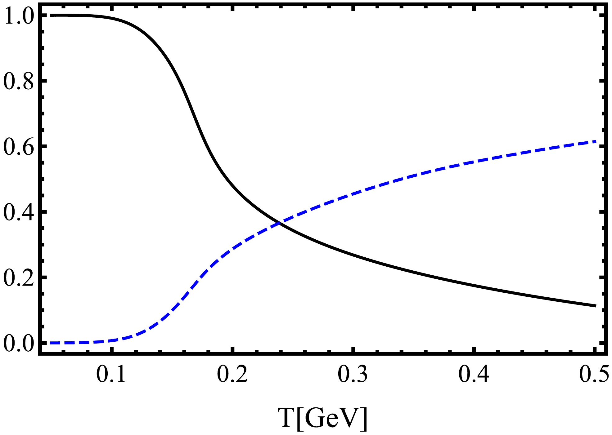
Figure 15. (color online) The normalized quark–antiquark condensate,
$ \langle\bar{\psi}{\psi}\rangle (T)/\langle\bar{\psi}{\psi}\rangle(0) $ , and the dPl,$ \Sigma_{1}(T)/\langle\bar{\psi}{\psi}\rangle(0) $ , are evaluated for a finite seed mass$ m_c = 7 $ MeV. The two quantities intersect at$ T_c\approx 0.22 $ GeV; thus, chiral-symmetry restoration and deconfinement occur at the same critical temperature,$ T_c $ . -
In lattice QCD, the confinement/deconfinement transition is typically studied by examining the behavior of the Polyakov loop (PL)
$ {\cal{P}} $ [16], which is the expectation value of a Wilson loop wrapping around the periodic Euclidean time direction. The Polyakov loop is explicitly defined as:$ {\cal{P}} = \frac{1}{N_{c}}\langle {\rm{Tr}}\left[ \Pi {\rm{e}}^{ {-\int^{1/T}_{0} {\rm d}\tau A_{0}}}\right] \rangle. $
(55) Here, Π represents the path ordering of the exponential, and
$ N_{c} $ is the number of colors. At finite T, the action S in the pure-gauge sector with gauge group$ S U(N_c) $ has a global$ Z(N_c) $ symmetry [68]. This symmetry is spontaneously broken, and the PL expectation value is considered the order parameter. This follows because we can write$ {\cal{P}} $ as:$ {\cal{P}} = {\rm e}^{-E_{q}(T)/T}\;. $
(56) The free energy of a single quark in a gluonic heat bath is denoted by
$ E_{q}(T) $ . In the confined phase, where$ \langle {\cal{P}}\rangle = 0 $ , corresponding to$ E_{q}(T)\rightarrow \infty $ , the quark is confined. In contrast, in the deconfined phase, where$ \langle {\cal{P}}\rangle\neq0 $ ,$ E_{q}(T) $ is finite, indicating that quarks are deconfined.A few years ago, another order parameter, referred to as the ''dual quark condensate'' or dPL, was introduced to explore the confinement–deconfinement phase transition in lattice [24, 25] and continuum SDE studies [27−30]. It has also been explored in variants of the NJL model [69−71] and QED3 [72]. The dPL is commonly denoted by
$ \Sigma_{n} $ and is defined as$ \Sigma_{n} = -\int^{2\pi}_{0}\frac{{\rm d}\phi}{2\pi} {\rm e}^{-{\rm i} n\phi} \langle\bar{\psi}\psi\rangle_{\phi}, $
(57) where n is an integer, and
$ \Sigma_{n} $ is the projection of$ \langle\bar{\psi}\psi\rangle_{\phi} $ onto loops winding n times around the temporal direction. The ϕ-dependent condensate can be obtained from the ϕ-dependent quark propagator as$ \langle \bar{\psi}\psi\rangle_{\phi} = N_{c}T\sum\limits_{n}\int \frac{{\rm d}^3\vec{k}}{(2\pi)^3}{\rm{Tr}}[S(\vec{k},\omega_{n}^{\phi})]. $
(58) The generalized condensate
$ \langle \bar{\psi}\psi\rangle_{\phi} $ is defined as the quark condensate evaluated for quark fields satisfying twisted boundary conditions:$ \psi(1/T,\vec{x}) = {\rm{e}}^{-{\rm i}\phi}\psi(0,\vec{x}), $
(59) in the imaginary-time direction, where
$ \phi\in[0,2\pi] $ . For$ \phi = \pi $ , the standard anti-periodicity of ψ can be retained. The above-mentioned$ U(1) $ -valued boundary conditions in momentum space yield generalized ϕ- dependent Matsubara frequencies,$ \omega_n\rightarrow \omega_{n}^{\phi} = (2n+ \phi/ \pi)\pi T $ , obtained by slightly modifying the usual fermionic Matsubara frequencies through the inclusion of a purely imaginary chemical potential,$ \mu_I = \phi T $ . From the lattice QCD perspective, it can be defined as a sum of Wilson loops winding n times around the temporal boundary [24, 25]. The shortest Pl with winding number$ n = 1 $ , considered as a collection of generalized Pl with spatial fluctuations, is referred to as the ''dressed Polyakov loop (dPl)'' [24, 25]$ \Sigma_1 = -\int^{2\pi}_{0}\frac{{\rm d}\phi}{2\pi} {\rm e}^{-{\rm i}\phi} \langle\bar{\psi}\psi\rangle_{\phi}. $
(60) $ \Sigma_{1} $ and the conventional Polyakov loop obey the same transformation properties; both transform identically under center transformations. Therefore,$ \Sigma_1 $ is considered an order parameter for the deconfinement phase transition. In the infinite-quark-mass limit, the Polyakov loop reduces to the chiral condensate because spatial fluctuations are suppressed. This relationship is connected to the ordinary quark condensate through boundary conditions. The dual Polyakov loop provides a potential link between the chiral and deconfinement phase transitions, possibly explaining why these transitions occur at nearly the same temperature [24, 25, 27, 28]. Another important feature of the dual Polyakov loop, denoted as$ \Sigma_{I} $ , is that it can be computed directly using lattice and functional methods.As noted above, Matsubara frequencies can be generalized by considering a theory with a purely imaginary chemical potential
$ \mu_I = \phi T $ . This equivalence follows from the symmetry of$ \langle\bar{\psi}\psi\rangle_{\phi} $ with respect to$ \phi = \pi $ , namely$ \langle\bar{\psi}\psi\rangle_{\phi-\pi} = \langle\bar{\psi}\psi\rangle_{\phi+\pi} $ . The value of$ \langle\bar{\psi}\psi\rangle_{\phi = \pi} $ corresponds to the conventional quark condensate. Therefore, it is preferable to express the Matsubara frequencies in terms of a theory with an imaginary chemical potential. Thus, we can write Eq. (61) as:$ \Sigma_1 = -\int^{\pi}_{0}\frac{{\rm d}\varphi}{\pi} {\rm{cos}}(\varphi) \langle\bar{\psi}\psi\rangle_{\varphi+\pi}. $
(61) The dPL and the conventional condensate obtained with the contact-interaction model at finite temperature [67] are shown in Fig. 15. The latter decreases as T increases up to
$ T_c $ , where it exhibits an inflection point, whereas the former increases most rapidly at approximately the same$ T_c $ . In QCD, this is precisely the expected behavior of both order parameters. Nevertheless, it has been observed [30] that this apparently universal behavior cannot be consistent with confinement in theories with trivial center symmetry; therefore, its appealing physical interpretation cannot be straightforwardly extended to effective models of QCD.
Figure 15. (color online) The normalized quark–antiquark condensate,
$ \langle\bar{\psi}{\psi}\rangle (T)/\langle\bar{\psi}{\psi}\rangle(0) $ , and the dPl,$ \Sigma_{1}(T)/\langle\bar{\psi}{\psi}\rangle(0) $ , are evaluated for a finite seed mass$ m_c = 7 $ MeV. The two quantities intersect at$ T_c\approx 0.22 $ GeV; thus, chiral-symmetry restoration and deconfinement occur at the same critical temperature,$ T_c $ . -
As mentioned earlier, in theories that lack center symmetry, the Polyakov and dressed Polyakov loops may not serve as effective order parameters for confinement/deconfinement. Instead, the confinement scale
$ \tilde{\tau}_{ir} $ provides an alternative order parameter for confinement in such theories [44]. The finite-temperature version of the CI model in Eq. (40) is given by$ M = m_0 + \frac{2M \alpha_{\rm{eff}}T}{3\pi^{3/2}} \int^{\tilde{\tau}^2_{ir}}_{\tau^2_{uv}}{\rm d}\tau \frac{ {\rm{e}}^{-M^2\tau}\Theta_{2}(0, {\rm{e}}^{-4\pi^2 T^2\tau})}{\tau^{3/2}}, $
(62) where
$ \Theta_{2}(0, x) $ denotes the second Jacobi theta function. The finite-temperature confinement length scale is given by [37, 38, 40−44]:$ \tilde{\tau}_{ir} = \tau_{ir}\frac{M(0)}{M(T)}. $
(63) The gap equation is solved at finite temperature in the chiral limit using the contact-interaction model, as shown in Fig. 16. The corresponding analysis for a current-quark mass of
$ m = 0.007 $ GeV is shown in Fig. 17.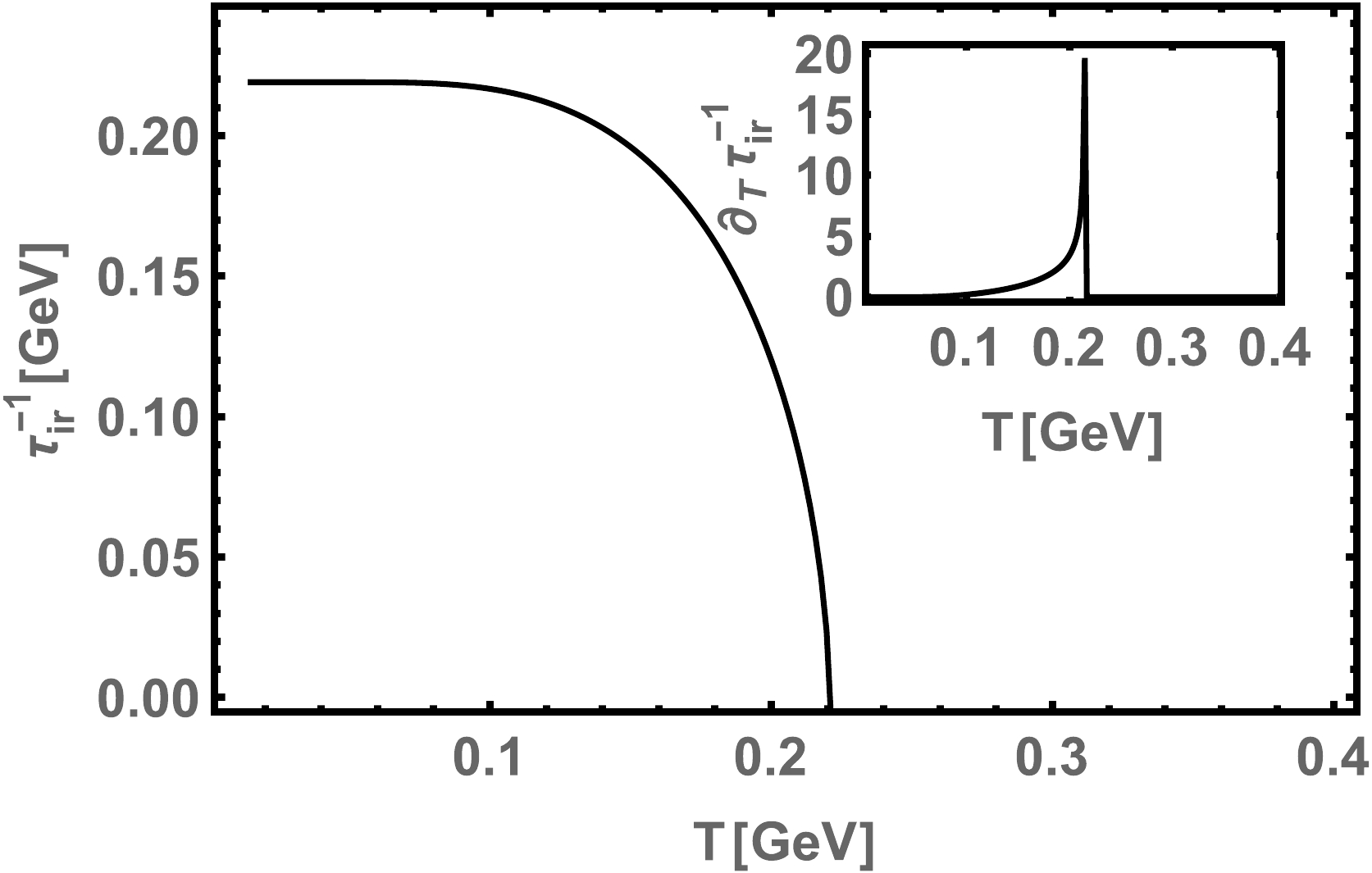
Figure 16. The inverse confinement length scale
$ \tau_{ir}^{-1} $ as a function of temperature T in the chiral limit. The main panel shows that the confinement scale decreases with increasing temperature. The inset shows the thermal derivative$ \partial_T \tau_{ir}^{-1} $ , whose sharp peak provides a precise definition of the critical temperature$ T_c $ for the deconfinement transition.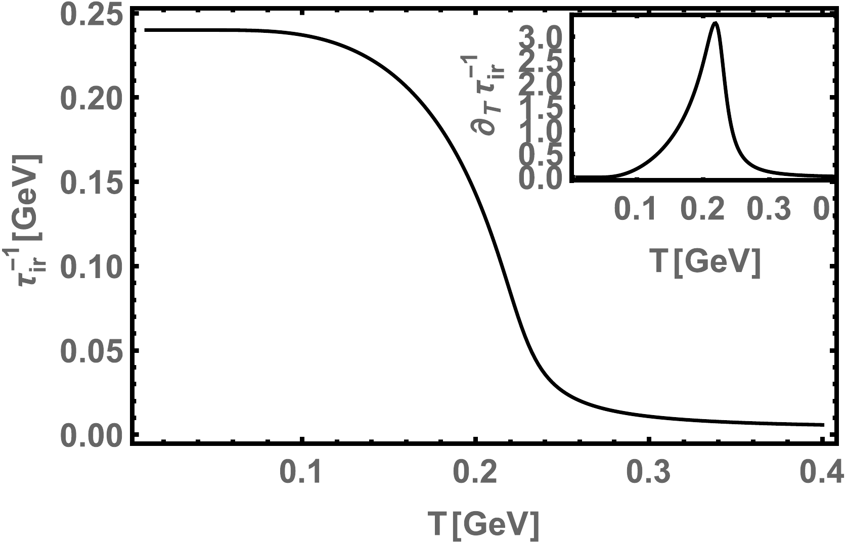
Figure 17. Temperature dependence of the confinement scale
$ \tau_{ir}^{-1} $ for a finite current quark mass. A comparison with Fig. 16 shows that a physical quark mass smooths the transition; the peak in the thermal gradient is broader and lower, indicating that the phase transition becomes a continuous crossover. -
As mentioned earlier, in theories that lack center symmetry, the Polyakov and dressed Polyakov loops may not serve as effective order parameters for confinement/deconfinement. Instead, the confinement scale
$ \tilde{\tau}_{ir} $ provides an alternative order parameter for confinement in such theories [44]. The finite-temperature version of the CI model in Eq. (40) is given by$ M = m_0 + \frac{2M \alpha_{\rm{eff}}T}{3\pi^{3/2}} \int^{\tilde{\tau}^2_{ir}}_{\tau^2_{uv}}{\rm d}\tau \frac{ {\rm{e}}^{-M^2\tau}\Theta_{2}(0, {\rm{e}}^{-4\pi^2 T^2\tau})}{\tau^{3/2}}, $
(62) where
$ \Theta_{2}(0, x) $ denotes the second Jacobi theta function. The finite-temperature confinement length scale is given by [37, 38, 40−44]:$ \tilde{\tau}_{ir} = \tau_{ir}\frac{M(0)}{M(T)}. $
(63) The gap equation is solved at finite temperature in the chiral limit using the contact-interaction model, as shown in Fig. 16. The corresponding analysis for a current-quark mass of
$ m = 0.007 $ GeV is shown in Fig. 17.
Figure 16. The inverse confinement length scale
$ \tau_{ir}^{-1} $ as a function of temperature T in the chiral limit. The main panel shows that the confinement scale decreases with increasing temperature. The inset shows the thermal derivative$ \partial_T \tau_{ir}^{-1} $ , whose sharp peak provides a precise definition of the critical temperature$ T_c $ for the deconfinement transition.
Figure 17. Temperature dependence of the confinement scale
$ \tau_{ir}^{-1} $ for a finite current quark mass. A comparison with Fig. 16 shows that a physical quark mass smooths the transition; the peak in the thermal gradient is broader and lower, indicating that the phase transition becomes a continuous crossover. -
Our study highlights that, unlike the chiral condensate, there is no universally agreed single order parameter for confinement in QCD and related theories. The behavior of the quark and gluon propagators, together with the axiom of reflection positivity, offers pathways for characterizing confinement within SDE frameworks. However, the precise link between pole structure and confinement remains unsettled in SDE solutions, whether inferred from spatial averages of these functions or from their inflection points.
It is worth mentioning that inflection points and zero-crossings derived from the propagator serve as indicators of confinement, but the propagator itself is computed within a specific model framework. Thus, inflection points and zero-crossings are suggestive rather than definitive; they signal confinement within the given model, but they do not constitute a universal proof. In this Schwinger-Dyson study of the Landau-gauge quark propagators in QCD at zero temperature, an inflection point in the scalar part of the propagator might be taken as indicative of confinement within that truncation. However, changing the truncation or gauge can remove or shift that inflection point, so the conclusion is strictly limited to that specific setup.
At finite temperature, the analytic structure of the quark propagator provides insight into the confinement/ deconfinement transition. In lattice studies, the Polyakov loop is considered the order parameter, although it is not directly calculated in the Schwinger-Dyson equations framework. However, its dressed variant is considered an approximate order parameter for center symmetry and is also naturally linked to the chiral condensate, although its status as a rigorous order parameter is theory- and model-dependent. This connection may explain why the
$ T_c $ values for chiral symmetry restoration and the deconfinement transition appear to coincide. However, a distinction must be maintained: the dressed Polyakov loop and the chiral condensate are closely linked to the symmetries of the QCD Lagrangian, namely center and chiral symmetry, respectively. Therefore, the dressed Polyakov loop can be viewed as an approximate order parameter when the theory possesses nontrivial center symmetry, despite its similar behavior in QCD, QED$ _3 $ , and NJL models.However, when the theory lacks center symmetry, it is difficult to associate the Polyakov and dressed Polyakov loops with confinement arguments based on the vacuum expectation values of these quantities. In contrast, a parameter such as the confining length scale
$ \tilde{\tau}_{ir} $ used in the momentum-independent CI truncation of the Schwinger-Dyson framework functions as a model-dependent proxy. While these proxies are highly successful in predicting hadron spectra, they do not provide a universal order parameter. In this momentum-independent setting, no gauge-invariant, dynamical confinement indicator is available. The confining length scale is introduced as a pragmatic surrogate to emulate confinement effects and to capture key qualitative features (e.g., the absence of colored asymptotic states and the emergence of deconfinement) within the CI truncation. Its value is not fundamental but is tuned to reproduce known phenomenology, and we discuss the associated limitations while outlining potential tests with more first-principles interactions.As noted earlier, the confining length scale is a model-dependent proxy introduced intentionally to mimic confinement within the chosen framework. It should be emphasized that, at finite temperature T, confinement is represented as long as this confinement length scale remains finite. However, at and above the critical temperature
$ (T_c) $ in the chiral limit, the CI model transitions to an ordinary NJL model, indicating a deconfinement transition with the development of poles in the propagator. The coincidence of$ T_c $ for chiral restoration and deconfinement, as indicated by various studies, including lattice simulations and the CI model, may reflect shared underlying dynamics rather than a fundamental equivalence of the two phenomena. The Polyakov-loop discussion supports this interpretation by highlighting that the confinement scale$ (\tilde{\tau}_{ir}) $ can also play the role of an order parameter for confinement in theories lacking center symmetry.Another relevant quantity is the continuum threshold parameter (
$ s_{0} $ ) [73], as used in finite energy sum rules. It defines the energy threshold at which states transition from discrete resonances to the perturbative quark-gluon continuum, signaling the deconfinement of hadrons. This quantity exhibits behavior similar to that of the Polyakov loop when connected with finite energy sum rules [74]. Its implementation in the SDE framework could shed light on whether chiral symmetry breaking and confinement are independent emergent phenomena in QCD.Consequently, a robust understanding of confinement should rely on multiple, complementary indicators (e.g., propagator analytic structure, dressed Polyakov loop behavior, center-symmetry considerations, and spectral features) rather than a single parameter.
Future work should aim to connect these indicators more tightly by exploring whether the independent emergence of chiral and confinement phenomena is possible in more complete frameworks and by clarifying the roles of quantities such as the Polyakov loop, the dressed Polyakov loop, and
$ \tilde{\tau}_{ir} $ across different gauge theories. This multifaceted approach may reveal whether confinement can ever be fully decoupled from chiral dynamics or whether their intertwined nature is an intrinsic property of non-Abelian gauge theories. -
Our study highlights that, unlike the chiral condensate, there is no universally agreed single order parameter for confinement in QCD and related theories. The behavior of the quark and gluon propagators, together with the axiom of reflection positivity, offers pathways for characterizing confinement within SDE frameworks. However, the precise link between pole structure and confinement remains unsettled in SDE solutions, whether inferred from spatial averages of these functions or from their inflection points.
It is worth mentioning that inflection points and zero-crossings derived from the propagator serve as indicators of confinement, but the propagator itself is computed within a specific model framework. Thus, inflection points and zero-crossings are suggestive rather than definitive; they signal confinement within the given model, but they do not constitute a universal proof. In this Schwinger-Dyson study of the Landau-gauge quark propagators in QCD at zero temperature, an inflection point in the scalar part of the propagator might be taken as indicative of confinement within that truncation. However, changing the truncation or gauge can remove or shift that inflection point, so the conclusion is strictly limited to that specific setup.
At finite temperature, the analytic structure of the quark propagator provides insight into the confinement/ deconfinement transition. In lattice studies, the Polyakov loop is considered the order parameter, although it is not directly calculated in the Schwinger-Dyson equations framework. However, its dressed variant is considered an approximate order parameter for center symmetry and is also naturally linked to the chiral condensate, although its status as a rigorous order parameter is theory- and model-dependent. This connection may explain why the
$ T_c $ values for chiral symmetry restoration and the deconfinement transition appear to coincide. However, a distinction must be maintained: the dressed Polyakov loop and the chiral condensate are closely linked to the symmetries of the QCD Lagrangian, namely center and chiral symmetry, respectively. Therefore, the dressed Polyakov loop can be viewed as an approximate order parameter when the theory possesses nontrivial center symmetry, despite its similar behavior in QCD, QED$ _3 $ , and NJL models.However, when the theory lacks center symmetry, it is difficult to associate the Polyakov and dressed Polyakov loops with confinement arguments based on the vacuum expectation values of these quantities. In contrast, a parameter such as the confining length scale
$ \tilde{\tau}_{ir} $ used in the momentum-independent CI truncation of the Schwinger-Dyson framework functions as a model-dependent proxy. While these proxies are highly successful in predicting hadron spectra, they do not provide a universal order parameter. In this momentum-independent setting, no gauge-invariant, dynamical confinement indicator is available. The confining length scale is introduced as a pragmatic surrogate to emulate confinement effects and to capture key qualitative features (e.g., the absence of colored asymptotic states and the emergence of deconfinement) within the CI truncation. Its value is not fundamental but is tuned to reproduce known phenomenology, and we discuss the associated limitations while outlining potential tests with more first-principles interactions.As noted earlier, the confining length scale is a model-dependent proxy introduced intentionally to mimic confinement within the chosen framework. It should be emphasized that, at finite temperature T, confinement is represented as long as this confinement length scale remains finite. However, at and above the critical temperature
$ (T_c) $ in the chiral limit, the CI model transitions to an ordinary NJL model, indicating a deconfinement transition with the development of poles in the propagator. The coincidence of$ T_c $ for chiral restoration and deconfinement, as indicated by various studies, including lattice simulations and the CI model, may reflect shared underlying dynamics rather than a fundamental equivalence of the two phenomena. The Polyakov-loop discussion supports this interpretation by highlighting that the confinement scale$ (\tilde{\tau}_{ir}) $ can also play the role of an order parameter for confinement in theories lacking center symmetry.Another relevant quantity is the continuum threshold parameter (
$ s_{0} $ ) [73], as used in finite energy sum rules. It defines the energy threshold at which states transition from discrete resonances to the perturbative quark-gluon continuum, signaling the deconfinement of hadrons. This quantity exhibits behavior similar to that of the Polyakov loop when connected with finite energy sum rules [74]. Its implementation in the SDE framework could shed light on whether chiral symmetry breaking and confinement are independent emergent phenomena in QCD.Consequently, a robust understanding of confinement should rely on multiple, complementary indicators (e.g., propagator analytic structure, dressed Polyakov loop behavior, center-symmetry considerations, and spectral features) rather than a single parameter.
Future work should aim to connect these indicators more tightly by exploring whether the independent emergence of chiral and confinement phenomena is possible in more complete frameworks and by clarifying the roles of quantities such as the Polyakov loop, the dressed Polyakov loop, and
$ \tilde{\tau}_{ir} $ across different gauge theories. This multifaceted approach may reveal whether confinement can ever be fully decoupled from chiral dynamics or whether their intertwined nature is an intrinsic property of non-Abelian gauge theories.
Confinement order parameters in QCD: a view from Schwinger–Dyson equations and related low energy QCD models
- Received Date: 2026-02-22
- Available Online: 2026-11-15
Abstract: Confinement and dynamical chiral symmetry breaking are two emergent non-perturbative phenomena of quantum chromodynamics (QCD) that are responsible for the nature of hadron spectra. While it is well known that the chiral condensate $ -\langle\bar{\psi} \psi \rangle $ is an order parameter for the chiral transition, the Polyakov loop is the associated approximate order parameter for the confinement–deconfinement transition in the pure gauge sector with center symmetry. Nevertheless, this quantity cannot be derived from functional methods, and other quantities have therefore been proposed as order parameters for this transition. In the current investigation, we review and compare several proposed parameters that have been used to describe the confinement/deconfinement transition in QCD and related quantum field theories in the framework of Schwinger–Dyson equations.



 DownLoad: