


 Abstract
 HTML
 Reference
 Related
 PDF


-
The observation of a Higgs boson with a mass of
$ 125\; {\rm{GeV}} $ at the Large Hadron Collider (LHC) in 2012 completed the particle spectrum of the Standard Model (SM), marking a major triumph of the theory. At the LHC, the dominant Higgs boson production mechanisms are gluon–gluon fusion ($ gg{\rm{F}} $ ), vector-boson fusion (VBF), associated production with a weak gauge boson ($ VH $ ), and associated production with a top-quark pair ($ t\bar{t}H $ ). Among these, the$ VH $ production mode plays a central role in the experimental observation of the$ H \rightarrow b\bar{b} $ decay at ATLAS [1] and CMS [2]. This is primarily because the accompanying W or Z boson, when decaying leptonically, provides clean and efficient trigger signatures while substantially suppressing the otherwise overwhelming multijet background. Moreover, the$ pp \rightarrow VH $ process is sensitive to the strength of the$ VVH $ coupling and is particularly well suited for probing potential deviations from SM predictions [3, 4]. As such, it constitutes a key channel for testing the gauge structure of the SM.At hadron colliders, the leading-order contribution to
$ VH $ associated production arises from Drell–Yan-type quark–antiquark annihilation. The QCD corrections to$ VH $ production have been computed up to next-to-next-to-next-to-leading order ($ {\rm{N}}^3{\rm{LO}} $ ) at the inclusive level [5], with next-to-next-to-leading order (NNLO) predictions available through the$ \mathrm{VH@NNLO} $ package [6−8], which is widely employed in precision phenomenology. The next-to-leading order (NLO) electroweak (EW) corrections have been calculated in Refs. [9, 10] and implemented in the$ \mathrm{HAWK} $ Monte Carlo program [11]. Combined NLO QCD and EW corrections are presented in Refs. [12, 13]. The NNLO QCD predictions for the differential distributions of$ WH $ and$ ZH $ production are available in Refs. [14, 15]. These fixed-order results have been matched to parton showers to achieve NNLO+PS accuracy in exclusive event simulations [16, 17], allowing for precise comparisons with experimental data. In the five-flavor scheme, the$ b\bar{b} \rightarrow ZH $ process, which incorporates a nonzero bottom-quark Yukawa coupling, has been computed at QCD NNLO within the soft-virtual approximation [18]. Moreover, the polarized$ q \bar{q} \rightarrow ZH $ amplitudes at two-loop order in QCD have been studied analytically in Ref. [19].The loop-induced process
$ gg \rightarrow ZH $ contributes at leading order with a cross section proportional to$ \alpha_s^2 $ , thereby constituting an NNLO QCD correction to the$ pp \rightarrow ZH $ process. However, owing to the large gluon luminosity at the LHC, this loop-induced channel contributes appreciably, representing approximately 10% of the total$ ZH $ cross section [20]. In the boosted regime, where the Higgs boson possesses large transverse momentum, this relative contribution is further enhanced [21, 22], making it a notable source of theoretical uncertainty. Moreover, because the amplitude depends on the particle content and couplings in the loops, this channel provides a particularly promising probe of potential new physics. The LO results for$ ZH $ production via gluon–gluon fusion were first presented in Refs. [23, 24]. The complete NLO QCD corrections were initially computed in the heavy-top limit ($ m_t \rightarrow +\infty $ ) [25], yielding a substantial enhancement of the cross section with a K-factor close to$ 2 $ ; the finite top-quark mass effects were subsequently analyzed using large-$ m_t $ expansions [26]. Two-loop virtual corrections computed via a transverse-momentum expansion are presented in Ref. [27], while results in the high-energy and large-$ m_t $ limits have been reported in Ref. [28]. Fully mass-dependent two-loop amplitudes have also been evaluated numerically [29]. Building on these results, full NLO QCD predictions have been further refined through a variety of expansion techniques, including small-$ m_H $ and$ m_Z $ expansions [30], combinations of sector decomposition with high-energy expansions [31], and hybrid approaches that integrate small-$ p_T $ and high-energy expansions to achieve comprehensive coverage of the phase space [32, 33].Although QCD corrections to the gluon-fusion channel in
$ ZH $ production have been extensively studied, a comprehensive analysis of the corresponding NLO EW corrections remains lacking. These corrections involve virtual contributions with a large number of diagrams that introduce an additional mass scale,$ m_W $ , rendering their computation highly nontrivial. In view of the increasingly precise experimental measurements, the accuracy of the theoretical prediction for the$ gg \rightarrow ZH $ process must also be further improved. The size of the NLO EW corrections for this process can be inferred qualitatively from existing results for related gluon-fusion processes with similar loop structures. For the loop-induced processes$ gg \rightarrow HH $ and$ gg \rightarrow \gamma \gamma $ , the relative NLO EW corrections amount to approximately −4% [34] and 1%–2% [35], respectively. For the$ gg \rightarrow gH $ process, which shares a similar final-state spin configuration with$ gg \rightarrow ZH $ , the corresponding corrections reach about 4% [36, 37]. These results indicate that the NLO EW corrections to$ gg \rightarrow ZH $ are also expected to be at the several-percent level, making them non-negligible in future high-precision predictions for this process.This study presents an analytic evaluation of the master integrals (MIs) for the NLO EW corrections to
$ gg \rightarrow ZH $ , focusing on the planar topologies with light-fermion loops. The calculation is performed within the framework of canonical differential equations, yielding analytic$ \epsilon $ -expansions of these integrals up to$ {\cal{O}}(\epsilon^4) $ . The coefficients are expressed in terms of Goncharov polylogarithms (GPLs) wherever feasible, and otherwise as one-fold integrals over GPLs. These analytic expressions provide essential inputs for the calculation of the complete NLO EW corrections to$ gg \rightarrow ZH $ . The rest of this paper is organized as follows. In Section II, we present the kinematics of$ gg \rightarrow ZH $ and introduce the topologies of the two-loop integrals involved. The differential-equations method adopted in our calculation is detailed in Section III. Sections IV and V are devoted to the analytic evaluation of the canonical bases for two family branches, respectively. In Section VI, we discuss the analytic extension to the topologies associated with the$ ZZH $ vertex and the analytic continuation to the physical region, and we validate our analytic expressions by comparing them with numerical results. Finally, a brief summary is provided in Section VII. -
In this work, we focus on the two-loop NLO EW virtual corrections to
$ ZH $ production via gluon–gluon fusion,$ g(p_{1}) + g(p_{2}) \rightarrow Z(p_{3}) + H(p_{4})\,, $
(1) where all four external momenta
$ p_i $ ($ i = 1, \ldots, 4 $ ) are defined as incoming. The amplitude for this$ 2 \rightarrow 2 $ scattering process can be conveniently expressed in terms of the Mandelstam invariants$ s = {(p_{1} + p_{2})}^{2}\,, \qquad t = {(p_{2} + p_{3})}^{2}\,, \qquad u = {(p_{1} + p_{3})}^{2}\,. $
(2) Momentum conservation and the on-shell conditions for the external momenta imply
$ s + t + u = m_Z^2 + m_H^2 $ . Using this relation, we adopt either$ \{s,\, t\} $ or$ \{u,\, t\} $ as the independent Mandelstam variables in the subsequent analysis, depending on the topology under consideration.For the
$ gg \rightarrow ZH $ process, a total of$ 132 $ irreducible two-loop Feynman diagrams induced by light quarks contribute to the NLO EW corrections. These diagrams can be systematically classified into eight distinct topologies: four involving the$ WWH $ vertex and four analogous ones in which the$ WWH $ vertex is replaced by$ ZZH $ . Figure 1 illustrates the first four topologies, which consist of two planar and two non-planar configurations. Only the planar diagrams are considered in the present calculation.
Figure 1. (color online) Four representative Feynman-diagram topologies contributing to the NLO EW virtual corrections to
$ gg \rightarrow ZH $ , induced by light quarks and involving the$ WWH $ vertex. Line styles denote particle species: solid black for light fermions, curly black for gluons, wavy pink for W bosons, wavy red for Z bosons, and dashed blue for Higgs bosons.Within dimensional regularization, the dimensionless two-loop four-point scalar Feynman integrals belonging to the family
$ {\cal{F}}(D_1, \dots, D_9) $ are conventionally defined as$ I(a_{1}, \ldots, a_{9}) = \dfrac{{\rm e}^{2 \epsilon \gamma_{E}}}{(Q^2)^{d - a}} \int \frac{{\rm d}^{d} l_{1}}{{\rm i} \pi^{d / 2}}\, \dfrac{{\rm d}^{d} l_{2}}{{\rm i} \pi^{d / 2}}\, \dfrac{1}{{D}_1^{a_1} \cdots D_{9}^{a_9}}\,, $
(3) where
$ \gamma_E $ denotes the Euler–Mascheroni constant,$ d = 4 - 2\epsilon $ specifies the spacetime dimension,$ a = a_1 + \cdots + a_9 $ , and Q is a characteristic scale introduced to make I dimensionless. The loop momenta are labeled$ l_1 $ and$ l_2 $ , and$ D_i $ ($ i = 1, \dots, 9 $ ) denote the propagators of the internal lines. For a given set of propagators$ \{D_i\} $ , all integrals with arbitrary indices$ \{a_i\} $ constitute an integral family. According to the signs of the propagator indices$ \{a_i\} $ , an integral family can be decomposed into sectors. To this end, we introduce a binary vector$ (s_1, \ldots, s_9) $ , with$ s_i \in \{0,\, 1\} $ , to label the sectors of the integral family$ {\cal{F}} $ . The sector$ {\cal{S}}_{{\cal{F}}}(s_1, \ldots, s_9) $ is defined as$ {\cal{S}}_{{\cal{F}}}(s_1, \ldots, s_9) = \Big\{ I(a_1, \ldots, a_9) \mid \Theta(a_i) = s_i,\, i = 1, \dots, 9 \Big\}\,, $
(4) where
$ \Theta(x) $ denotes the Heaviside step function, defined by$ \Theta(x)=1 $ for$ x>0 $ and$ \Theta(x)=0 $ for$ x\leqslant 0 $ . A sector$ {\cal{S}}_{{\cal{F}}}(s_1, \ldots, s_9) $ is called a sub-sector of$ {\cal{S}}_{{\cal{F}}}(t_1, \ldots, t_9) $ if$ s_i \leqslant t_i $ for all$ i = 1, \ldots, 9 $ . The union of$ {\cal{S}}_{{\cal{F}}}(s_1, \ldots, s_9) $ and all its sub-sectors defines the branch induced by$ {\cal{S}}_{{\cal{F}}}(s_1, \ldots, s_9) $ , denoted by$ {\cal{B}}_{{\cal{F}}}(s_1, \ldots, s_9) $ . The four topologies associated with the$ WWH $ vertex shown in Fig. 1 fall into two distinct integral families:1. Family
$ {\cal{F}}_1 $ :$ \begin{aligned}[b] & D_{1} = l_{1}^{2}, && D_{2} = (l_{1} + p_{1})^{2}, && D_{3} = (l_{1} - p_{3} - p_{4})^{2} ,\\ & D_{4} = (l_{1} - p_{4})^{2}, && D_{5} = (l_{2} - p_{4})^{2} - m_{W}^{2}, && D_{6} = l_{2}^{2} - m_{W}^{2}, \\ & D_{7} = (l_{1} - l_{2})^{2}, && D_{8} = (l_{1} - l_{2} - p_{3})^{2}, && D_{9} = (l_{2} + p_{1})^{2}, \end{aligned} $
(5) two topologies
$ \subset {\cal{F}}_1 $ :$ \begin{split} {\cal{S}}_1 \equiv \;& {\cal{S}}_{{\cal{F}}_1}(1, 1, 1, 1, 1, 1, 1, 0, 0)\,, \\ {\cal{S}}_{1N} \equiv \;& {\cal{S}}_{{\cal{F}}_1}(1, 1, 1, 0, 1, 1, 1, 1, 0), \end{split} $
(6) 2. Family
$ {\cal{F}}_2 $ :$ \begin{aligned}[b] & D_{1} = l_{1}^{2}, && D_{2} = (l_{1} + p_{1})^{2}, && D_{3} = (l_{1} - p_{2} - p_{4})^{2}, \\ & D_{4} = (l_{1} - p_{4})^{2}, && D_{5} = (l_{2} - p_{4})^{2} - m_{W}^{2}, && D_{6} = l_{2}^{2} - m_{W}^{2}, \\ & D_{7} = (l_{1} - l_{2})^{2}, && D_{8} = (l_{1} - l_{2} + p_{1})^{2}, && D_{9} = (l_{2} + p_{2})^{2}, \end{aligned} $
(7) two topologies
$ \subset {\cal{F}}_2 $ :$ \begin{split} {\cal{S}}_{2} \equiv \;&{\cal{S}}_{{\cal{F}}_2}(1, 1, 1, 1, 1, 1, 1, 0, 0)\,,\\ {\cal{S}}_{2N} \equiv \;& {\cal{S}}_{{\cal{F}}_2}(0, 1, 1, 1, 1, 1, 1, 1, 0), \end{split} $
(8) Here,
$ {\cal{S}}_1 $ and$ {\cal{S}}_2 $ correspond to the planar topologies shown in Fig. 1, which are evaluated analytically in this work, whereas$ {\cal{S}}_{1N} $ and$ {\cal{S}}_{2N} $ denote the remaining two non-planar topologies.Integration-by-parts (IBP) [38, 39] identities establish linear relations among integrals within a given branch of an integral family, with coefficients that are rational functions of the external kinematic invariants and internal masses. These relations allow all integrals in a given branch to be reduced to a finite set of master integrals (MIs) [40]. For convenience, we denote the branch induced by
$ {\cal{S}}_1 $ as$ {\cal{B}}_1 $ , and that induced by$ {\cal{S}}_2 $ as$ {\cal{B}}_2 $ . Using the$ \mathrm{Kira} $ package [41, 42], which implements the Laporta algorithm [43], we have reduced the integrals in$ {\cal{B}}_{1} $ and$ {\cal{B}}_{2} $ to$ 62 $ and$ 59 $ MIs, respectively. -
The derivative of any scalar Feynman integral with respect to kinematic invariants can be reduced, via IBP identities, to linear combinations of integrals within the same family branch, implying that the branch is closed under differentiation with respect to these invariants. Consequently, the corresponding MIs satisfy a closed system of linear differential equations in these variables. We use
$ \mathrm{LiteRed} $ [44, 45] to perform the differentiation and$ \mathrm{Kira} $ to carry out the reduction, thereby obtaining a coupled system of linear differential equations satisfied by the MIs. However, obtaining analytic solutions to such multivariable systems of differential equations is, in general, a highly nontrivial task. If there exists a basis$ \vec{g}(\vec{x}, \epsilon) $ in which the differential equations can be cast into a canonical (or$ \epsilon $ -factorized) form,$ {\rm d} \vec{g}(\vec{x}, \epsilon) = \epsilon\, {\rm d} \mathbb{A}(\vec{x})\, \vec{g}(\vec{x}, \epsilon)\,, $
(9) the system simplifies considerably, and its solution can be expressed in terms of Chen's iterated integrals [46],
$ \vec{g}(\vec{x}, \epsilon) = {\cal{P}} \exp\Big(\epsilon \int_{\gamma} {\rm d} \mathbb{A}\Big)\, \vec{g}(\vec{x}_0, \epsilon)\,, $
(10) where
$ {\cal{P}} $ denotes the path-ordering operator, and γ is an integration path connecting$ \vec{x}_0 $ to$ \vec{x} $ . This approach is known as the canonical differential-equations method [47], and the corresponding set of MIs is referred to as a canonical basis. Several approaches have been developed for constructing a canonical basis, including the Magnus expansion [48−50],$ {\rm d}\log $ integrand construction [51], intersection theory [52, 53], and leading singularity analysis [47, 54]. In this work, the canonical basis is constructed via the Magnus expansion starting from a linear basis.Let
$ \vec{f}(\vec{x}, \epsilon) $ be a linear basis of a family branch of Feynman integrals satisfying the following system of differential equations:$ \partial_i \vec f(\vec{x}, \epsilon) = \Big[\, \mathbb{B}_i^{(0)}(\vec{x}) + \epsilon\, \mathbb{B}_i^{(1)}(\vec{x}) \,\Big]\, \vec{f}(\vec{x}, \epsilon)\,, \qquad (i = 1, \ldots, n)\,, $
(11) where
$ \partial_i \equiv \partial/\partial x_i $ and$ \vec{x} = (x_1, \ldots, x_n) $ . We introduce the matrix$ \mathbb{T} $ , defined recursively as follows:$ \begin{aligned}[b] \mathbb{T} = \mathbb{T}_n\,, \end{aligned} \quad\; \left\lbrace \begin{aligned}\mathbb{T}_i =& \mathbb{T}_{i-1} \exp\Big( \Omega_i \big[ \widetilde{\mathbb{B}}_i^{(0)} \big] \Big) \; \; {\rm{with}}\; \; \widetilde{\mathbb{B}}_i^{(0)} \\ &= \mathbb{T}_{i-1}^{-1}\, \mathbb{B}_i^{(0)}\, \mathbb{T}_{i-1} \quad (i = 1, \ldots, n), \\ \mathbb{T}_0 =& 1_{n \times n} \end{aligned} \right. $
(12) where
$ \Omega_i $ denotes a family of matrix-valued functionals indexed by$ i \in \{1,\dots,n\} $ , each admitting a series representation known as the Magnus expansion [50],$ \begin{aligned}[b] \Omega_i\big[ \mathbb{F} \big](\vec{x}) =& \int^{x_i} {\rm d}x_i^{\prime}\, \mathbb{F}(\cdots,\,x_{i-1},\, x_i^{\prime},\, x_{i+1},\, \cdots) \\ &+ \frac{1}{2!} \int^{x_i} {\rm d}x_i^{\prime} \int^{x_i^{\prime}} {\rm d}x_i^{\prime\prime}\, \big[\, \mathbb{F}(\cdots,\,x_{i-1},\, x_i^{\prime},\, x_{i+1},\, \cdots)\,,\big.\\ &\quad \big.\mathbb{F}(\cdots,\,x_{i-1},\, x_i^{\prime\prime},\, x_{i+1},\, \cdots) \,\big] + \cdots \end{aligned} $
(13) The matrix
$ \mathbb{T} $ is invertible, and the transformation$ \mathbb{T}^{-1} $ maps the linear basis$ \vec{f\,} $ to the canonical basis$ \vec{g} = \mathbb{T}^{-1}\vec{f\,} $ . The recursive construction of this transformation is validated by the integrability conditions of the linear differential system (11). Consequently, the canonical basis$ \vec{g} $ satisfies the total differential equation (9), with$ {\rm d}\mathbb{A} $ given by$ {\rm d}\mathbb{A} = \sum\limits_{i=1}^{n} \mathbb{T}^{-1} \mathbb{B}_i^{(1)} \mathbb{T}\, {\rm d}x_i\,. $
(14) The differential one-form
$ {\rm d}\mathbb{A} $ can be expressed in$ {\rm d}\log $ form,$ {\rm d} \mathbb{A}(\vec{x}) = \sum\limits_a\, \mathbb{M}_a\, {\rm d} \log{\omega_a(\vec{x})}\,, $
(15) where
$ \mathbb{M}_a $ are constant matrices, and$ \omega_a $ , referred to as symbol letters, are algebraic functions of$ \vec{x} $ that collectively constitute the alphabet of the canonical differential system. Consequently, the recursion relations governing the coefficients in the$ \epsilon $ -expansion of the path-ordered integral representation of$ \vec{g}(\vec{x}, \epsilon) $ take the form$ \begin{split} \vec g^{\,(p)}(\vec{x}) =& \vec g^{\,(p)}(\vec{x}_0) \\ &+ \int_0^1 \sum\limits_a \mathbb{M}_a\, \frac{{\rm d} \log \omega_a(\vec{x}(t))}{{\rm d}t} \, \vec{g}^{\,(p-1)}(\vec{x}(t))\, {\rm d}t\,,\\ &\;\; p = 1, 2, \ldots \end{split} $
(16) where
$ \vec{x}(t) $ parametrizes an integration path from$ \vec{x}_0 $ to$ \vec{x} $ , such that$ \vec{x}(0) = \vec{x}_0 $ and$ \vec{x}(1) = \vec{x} $ . If the alphabet consists of rational letters, the$ {\rm d}\log $ kernels in the integral representation of$ \vec{g}^{\,(p)} $ reduce to rational functions with simple poles. The corresponding iterated integrals can therefore be expressed in terms of GPLs, which are defined recursively as$ G(a_n, \ldots, a_1; z) = \int_0^z \frac{{\rm d}z^{\prime}}{z^{\prime} - a_n}\, G(a_{n-1}, \ldots, a_1; z^{\prime})\,, $
(17) with
$ G(\, ; z) = 1 $ and$ G(\vec{0}_n; z) = \log^n (z) / n! $ . -
The Feynman integrals in the
$ {\cal{B}}_{1} $ branch depend on five independent kinematic invariants with dimensions of mass squared, which we take to be$ \big\{ s,\, t,\, m_Z^2,\, m_H^2,\, m_W^2 \big\} $ . After fixing the characteristic scale to$ Q = m_W $ , the dimensionless integrals can be conveniently parameterized in terms of the following dimensionless kinematic variables:$ x = -\, \dfrac{s}{m_W^2}\,, \quad y = -\, \dfrac{t}{m_W^2}\,, \quad z = -\, \dfrac{m_Z^2}{m_W^2}\,, \quad w = -\, \dfrac{m_H^2}{m_W^2}\,, $
(18) which we collectively denote by the vector
$ \vec{x} = (x, y, z, w) $ . The minus signs are introduced to ensure that all variables x, y, z, and w remain positive in the Euclidean region defined as$ {\cal{R}}_{{\rm{E}}} = \Big\{\, (x, y, z, w) \in \mathbb{R}^4 \;\Big|\; x \gt 0,\; y \gt 0,\; z \gt 0,\; w \gt 0 \,\Big\}\,. $
(19) Our analytical procedure begins with the following linear basis, assembled into the vector
$ \vec{f\,} $ :$ \begin{aligned}[b] f_{1} &= \epsilon\, \left(1 -\epsilon \right)I_{1}\,,& f_{2} &= \epsilon^{2} I_{2}\,,& f_{3} &= \epsilon^{2} I_{3}\,, & f_{4} &= \epsilon^{2} I_{4}\,,&\qquad f_{5} &= \epsilon^{2} I_{5}\,, &f_{6} &= \epsilon^{2} I_{6}\,,\\ f_{7} &= \epsilon^{2} I_{7}\,, & f_{8} &= \epsilon^{2} I_{8}\,,& f_{9} &= \epsilon^{2} I_{9}\,, & f_{10} &= \epsilon^{2} I_{10}\,, & f_{11} &= \epsilon^{2} I_{11}\,, & f_{12} &= \epsilon^{2} I_{12}\,,\\ f_{13} &= \epsilon^{2} I_{13}\,, & f_{14} &= \epsilon^{2} I_{14}\,, & f_{15} &= \epsilon^{3}\, (1 - 2\epsilon)\, I_{15}\,, & f_{16} &= \epsilon^{2}\, (1 - 2\epsilon)\, I_{16}\,,& f_{17} &= \epsilon^{2} I_{17}\,, & f_{18} &= \epsilon^{2} I_{18}\,, \\ f_{19} &= \epsilon^{2} I_{19}\,, & f_{20} &= \epsilon^{3} I_{20}\,, &f_{21} &= \epsilon^{3} I_{21}\,, & f_{22} &= \epsilon^{3} I_{22}\,, & f_{23} &= \epsilon^{3} I_{23}\,, & f_{24} &= \epsilon^{3} I_{24}\,, \\ f_{25} &= \epsilon^{2} I_{25}\,, &f_{26} &= \epsilon^{2} I_{26}\,, & f_{27} &= \epsilon^{2} I_{27}\,, & f_{28} &= \epsilon^{2} I_{28}\,, &f_{29} &= \epsilon^{2} I_{29}\,, & f_{30} &= \epsilon^{3} I_{30}\,, \\ f_{31} &= \epsilon^{3} I_{31}\,, & f_{32} &= \epsilon^{2}\, (1 - 2\epsilon)\, I_{32}\,, & f_{33} &= \epsilon^{2}\, (1 - 2\epsilon)\, I_{33}\,, & f_{34} &= \epsilon^{4} I_{34}\,, & f_{35} &= \epsilon^{4} I_{35}\,, & f_{36} &= \epsilon^{4} I_{36}\,,\\f_{37} &= \epsilon^{4} I_{37}\,, & f_{38} &= \epsilon^{3} I_{38}\,, & f_{39} &= \epsilon^{3} I_{39}\,, & f_{40} &= \epsilon^{3} I_{40}\,,& f_{41} &= \epsilon^{3} I_{41}\,, & f_{42} &= \epsilon^{3} I_{42}\,, \\ f_{43} &= \epsilon^{3} I_{43}\,, & f_{44} &= \epsilon^{3} I_{44}\,,&f_{45} &= \epsilon^{3} I_{45}\,, &f_{46} &= \epsilon^{3} I_{46}\,, & f_{47} &= \epsilon^{4} I_{47}\,, & f_{48} &= \epsilon^{3} I_{48}\,, \\ f_{49} &= \epsilon^{3} I_{49}\,, & f_{50} &= \epsilon^{4} I_{50}\,, & f_{51} &= \epsilon^{3} I_{51}\,, & f_{52} &= \epsilon^{3}\, (1 - 2\epsilon)\, I_{52}\,,& f_{53} &= \epsilon^{3}\, (1 - 2\epsilon)\, I_{53}\,, & f_{54} &= \epsilon^{3} I_{54}\,, \\ f_{55} &= \epsilon^{3} I_{55}\,, &f_{56} &= \epsilon^{4} I_{56}\,, &f_{57} &= \epsilon^{4} I_{57}\,, & f_{58} &= \epsilon^{3} I_{58}\,, & f_{59} &= \epsilon^{3} I_{59}\,, & f_{60} &= \epsilon^{3} I_{60}\,, \\ f_{61} &= \epsilon^{3} I_{61}\,, & f_{62} &= \epsilon^{4} I_{62}\,, \\[-10pt]\end{aligned} $
(20) where the MIs
$ I_i \; (i = 1, \ldots, 62) $ are displayed in Fig. 2. The differential equations for$ \vec{f\,} $ are derived by differentiation followed by IBP reduction, as detailed in Section III. After applying a Magnus transformation to the linear basis$ \vec{f\,} $ , the$ {\cal{O}}(\epsilon^0) $ terms in the coefficient matrices of the differential equations are eliminated, thereby yielding the canonical basis$ \vec{g} $ :
Figure 2. (color online) Pre-canonical basis for the
$ {\cal{B}}_1 $ branch. Line colors follow the same convention as in Fig. 1. Each dot on a propagator indicates an increment of one in the power of that propagator. The label$ (D_i) $ in the upper-left corner indicates that propagator$ D_i $ carries power$ -1 $ , while the labels adjacent to the thick gray external lines specify the corresponding kinematic invariants.$ \begin{aligned}[b] \begin{array}{*{20}{l}} g_{1} = f_{1}\,, & g_{2} = x\, f_{2}\,, & g_{3} = y\, f_{3}\,, & g_{4} = z\, f_{4}\,, \\ g_{5} = w\, f_{5}\,,&g_{6} = w r_{1}\, f_{6}\,, & g_{7} = x\, f_{7}\,, & g_{8} = y\, f_{8}\,, \\ g_{9} = z\, f_{9}\,, & g_{10} = w\, f_{10}\,,&g_{11} = 2\, f_{7} + (1+x)\, f_{11}\,, & g_{12} = 2\, f_{8} + (1+y)\, f_{12}\,,\\ g_{13} = 2\, f_{9} + (1+z)\, f_{13}\,, & g_{14} = 2\, f_{10} + (1+w)\, f_{14}\,, & g_{15} = w\, f_{15}\,, & g_{16} = { r_{1}/(4+w) \displaystyle \sum\nolimits_{i} \alpha_{16,i}\, f_{i}}\,, \\ g_{17} = y r_{1}\, f_{17}\,, & g_{18} = z r_{1}\, f_{18}\,, & g_{19} = x r_{1}\, f_{19}\,, & g_{20} = r_{2}\, f_{20}\,,\\ g_{21} = r_{1} r_{2}\, f_{21}\,, & g_{22} = (y-w)\, f_{22}\,, & g_{23} = r_{2}\, f_{23}\,, & g_{24} = r_{2}\, f_{24}\,, \\ g_{25} = (y-w)\, f_{25}\,, & g_{26} = r_{2}\, f_{26}\,, & g_{27} = r_{2}\, f_{27}\,,\\ g_{28} = 3\, (x-z+w)\, f_{23} + 2\, (x-z+w)\, & f_{26} + 2 x w\, f_{28}\,,&&&\\ g_{29} = 3\, (x+z-w)\, f_{24} + 2\, (x+z-w)\,& f_{27} + 2 x z\, f_{29}\,, &&&\\ g_{30} = (y-w)\, f_{30}\,,& g_{31} = r_{2}\, f_{31}\,, & g_{32} = { r_{1}/w \displaystyle \sum\nolimits_{i} \alpha_{32,i}\, f_{i}}\,, & g_{33} = { r_{1}/w \displaystyle \sum\nolimits_{i} \alpha_{33,i}\, f_{i}}\,, \\ g_{34} = (y-w)\, f_{34}\,, &g_{35} = (y-w)\, f_{35}\,, & g_{36} = r_{2}\, f_{36}\,, & g_{37} = r_{2}\, f_{37}\,,\\ g_{38} = y\, (y-w)\, f_{38}\,, &g_{39} = z r_{2}\, f_{39}\,, & g_{40} = x r_{2}\, f_{40}\,, & g_{41} = (y-w)\, r_{1}\, f_{41}\,,\\ g_{42} = r_{1} r_{2}\, f_{42}\,, &g_{43} = r_{1} r_{2}\, f_{43}\,, & g_{44} = 2 w\, f_{35} - y\, f_{44}\,, & g_{45} = { \displaystyle \sum\nolimits_{i} \alpha_{45,i}\, f_{i}}\,, \\ g_{46} = { \displaystyle \sum\nolimits_{i} \alpha_{46,i}\, f_{i}}\,, & g_{47} = w r_{2}\, f_{47}\,, & g_{48} = x y\, f_{48}\,, & g_{49} = x y r_{1}\, f_{49}\,, \\ g_{50} = (x+y-z)\, f_{50}\,, &g_{51} = (x+y-z+x y)\, f_{51}\,, &g_{52} = x\, ( f_{52} - f_{54} )\,, & g_{53} = (y-z)\, ( f_{53} - f_{55} )\,, \\ g_{54} = x y\, f_{54}\,, &g_{55} = x y\, f_{55}\,,& g_{56} = x\, (y-w)\, f_{56}\,, &&\\ g_{57} = [\, x y - (y-z) w \,]\, f_{57}\,, &g_{58} = x\, [\, 2 y\, f_{56} + (w+2y+wy)\, & f_{58} + (2 y-w)\, f_{60} \,]\,, &&\\ g_{59} = 2w\, (y-z)\, f_{57} + [\, w\, (y-z) + x y\,& (2+w) \,]\, f_{59} + [\, 2 x y - w\, (y-z) \,]\,& f_{61}\,, &&\\ g_{60} = x r_{1}\, [\, 2\, f_{56} + (1+y)\, f_{58} + f_{60} \,]\,, &&&&\\ g_{61} = r_{1}\, [\, 2\, (y-z)\, f_{57} + (y-z+x y)\, f_{59} & + (y-z)\, f_{61} \,]\,,&&& \\ g_{62} = w\, [\, x\, f_{56} + (y-z)\, f_{57} + x y\, f_{62} \,]\,, & & & & \\[-20pt] \end{array} \end{aligned} $
(21) where the non-vanishing coefficients
$ \alpha_{i,j} $ are given in Appendix A. The two square roots that appear in this canonical basis, denoted by$ r_1 $ and$ r_2 $ , are defined by$ r_1^2 = w\, (4 + w)\,, \qquad\quad r_2^2 = \lambda(x,\, z,\, w)\,, $
(22) where the Källén function λ is given by
$ \lambda(x,\, y,\, z) = x^2 + y^2 + z^2 - 2 x y - 2 y z - 2 z x\,. $
(23) The differential one-form matrix corresponding to the canonical basis
$ \vec{g} $ is obtained via the similarity transformation in Eq. (14). This matrix, in turn, determines the alphabet, which comprises$ 24 $ even and$ 12 $ odd letters [55]:● even letters
$ \begin{aligned}[b] \omega_{1} =& x\,,& \omega_{7} =& 1+z\,, &\omega_{13} =& y-z+x\,,& \omega_{19} =& xy-(y-z)\,w\,,\\ \omega_{2} =& y\,,&\omega_{8} =& 1+w\,,& \omega_{14} =& y-z+xy\,,&\omega_{20} =& xy+(y-z)\, (y-w)\,, \\ \omega_{3} =& z\,, &\omega_{9} =& 4+w\,, & \omega_{15} =& y-z+x\,(1+y)\,,&\omega_{21} =& (x-z)^{2}-w\, (1+x)\, (1+z)\,, \\ \omega_{4} =& w\,,&\omega_{10} =& y-z\,, &\omega_{16} =& y^{2}-w\,(1+y)\,,& \omega_{22} =& r_2^2\,, \\ \omega_{5} =& 1+x\,,& \omega_{11} =& y-w\,, &\omega_{17} =& (1+z)\, (1+w)-x\,, & \omega_{23} =& (x+y-z)^{2} + xw\, (y-z)\,, \\ \omega_{6} =& 1+y\,,& \omega_{12} =& 1-y+w\,, & \omega_{18} =& (1+x)\, (1+w)-z\,,&\omega_{24} =& x^{2} y^{2}-w\,(y-z)\, (xy+y-z)\,, \end{aligned} $
(24) ● odd letters
$ \begin{aligned}[b] \omega_{25} &= \frac{w+r _{1}}{w-r _{1}}\,, &\omega_{29} &= \frac{2w\,(y-z)+xy\, (w+r _{1})}{2w\,(y-z)+xy\, (w-r _{1})}\,,& \omega_{33} &= \frac{2+x-z+w+r _{2}}{2+x-z+w-r _{2}}\,,\\ \omega_{26} &= \frac{2y-w+r _{1}}{2y-w-r _{1}}\,, & \omega_{30} &= \frac{x-z-w+r _{2}}{x-z-w-r _{2}}\,, &\omega_{34} &= \frac{x+2y-z-w+r _{2}}{x+2y-z-w-r _{2}}\,, \\ \omega_{27} &= \frac{w\,(2+x+z)+(x-z)\, r _{1}}{w\,(2+x+z)-(x-z)\, r _{1}}\,, & \omega_{31} &= \frac{x-z+w+r _{2}}{x-z+w-r _{2}}\,, & \omega_{35} &= \frac{(1-z)\, (x-z)-(1+z)\, (w-r _{2})}{(1-z)\, (x-z)-(1+z)\, (w+r _{2})}\,, \\ \omega_{28} &= \frac{2\, (y-z)+x\, (2+w+ r _{1})}{2\, (y-z)+x\, (2+w- r _{1})}\,, & \omega_{32} &= \frac{2-x+z+w+r _{2}}{2-x+z+w-r _{2}}\,,&\omega_{36} &= \frac{w\, (2-x-z+w)+r _{1} r _{2}}{w\, (2-x-z+w)-r _{1} r _{2}}\,.\end{aligned} $
(25) Expressing the iterative solutions of the canonical basis in terms of GPLs typically requires rationalizing the square roots in the alphabet. For
$ {\cal{B}}_1 $ , although both$ r_1 $ and$ r_2 $ can be simultaneously rationalized by an appropriate transformation, this is unnecessary because not all MIs depend on both square roots. A more efficient strategy is therefore to treat subsystems characterized by distinct radical structures separately and rationalize each subsystem individually. In the following, we demonstrate how to determine the dependence of each MI in a given family branch on a specified set of square roots, which serves as the basis for constructing the corresponding subsystems.To characterize the radical structure of the MIs, we introduce the radical index
$ {\cal{Z}}_{r_1,\ldots,r_N} $ . It is an N-bit binary number that encodes the dependence of a function on the set of independent square roots$ \{r_1, \ldots, r_N\} $ , and is defined as$ {\cal{Z}}_{r_1,\ldots,r_N}\left[\, h \,\right] = (\mu_1 \ldots \mu_N) \;\;\; {\rm{with}} \;\;\; \mu_i = \begin{cases} \;0\,, & {\rm{if}} \quad h\,|_{\,r_i \; \longrightarrow\; -r_i} = h, \\ \;1\,, & {\rm{if}} \quad h\,|_{\,r_i \; \longrightarrow\; -r_i} \neq h, \end{cases} $
(26) For a composite expression, the dependence on each root accumulates as the constituent components are combined. This accumulated dependence is captured by the binary operation bitwise OR, denoted by
$ | $ , which is defined as follows:$ (\mu_1 \ldots \mu_N) \,\big|\, (\nu_1 \ldots \nu_N) = (\lambda_1 \ldots \lambda_N)\,, \quad\; {\rm{where}} \quad\; \lambda_i = \max\{\mu_i\,, \nu_i\}\,. $
(27) It then follows that
$ {\cal{Z}}_{r_1,\ldots,r_N}\left[\, h_1 \smile h_2 \,\right] \leqslant {\cal{Z}}_{r_1,\ldots,r_N}\left[\, h_1 \,\right] \,\big|\, {\cal{Z}}_{r_1,\ldots,r_N}\left[\, h_2 \,\right]\,, $
(28) where
$ h_1 \smile h_2 $ denotes any fundamental arithmetic operation on$ h_1 $ and$ h_2 $ , i.e., addition, subtraction, multiplication, or division. Note that this equality holds in general, except when cancellations occur between square roots, including degenerate cases where either$ h_1 $ or$ h_2 $ vanishes.The zeroth-order MIs are constants; consequently, their radical indices are zero. According to the recursion relation (16), the radical index of a canonical MI at any order is determined by performing a bitwise OR on the radical indices of all nonzero elements of
$ {\rm d}\mathbb{A} $ involved in the iteration, together with those of the corresponding nonzero MIs from the preceding order, namely$ {\cal{Z}}_{r_1,\ldots,r_N}\big[\, g_i^{(p)} \,\big] = \Big|_{\,j:\; {\rm d}\mathbb{A}_{ij} g_j^{(p-1)} \neq 0} \Big( {\cal{Z}}_{r_1,\ldots,r_N}\big[\, {\rm d}\mathbb{A}_{ij} \,\big] \,\big|\, {\cal{Z}}_{r_1,\ldots,r_N}\big[\, g_j^{(p-1)} \,\big] \Big)\,. $
(29) Equation (29) defines a tree-like structure for efficiently computing the radical index for each canonical MI. Since loops are permitted in this structure, we refer to it as a tropical tree. Each node in a tropical tree represents a canonical MI, and each edge corresponds to a nonzero element of
$ {\rm d}\mathbb{A} $ . The tree expands layer by layer, with each layer of nodes generating new nodes simultaneously via the edges, continuing until no additional distinct nodes are produced. We denote the tropical tree rooted at$ g_i $ as$ \mathrm{Tree} $ ($ g_i $ ) and the set of all its nodes as$ \mathtt{Node} $ ($ g_i $ ). Evidently,$ \mathtt{Node} $ ($ g_i $ ) defines the minimal subsystem that contains the MI$ g_i $ , and the radical index of$ g_i $ is given by$ {\cal{Z}}_{r_1,\ldots,r_N}\left[\, g_i \,\right] = \Big|_{\,j:\; g_j \in\, \mathtt{Node}\ {( g_i )}} \Big(\, \Big|_{\,k:\; {\rm d}\mathbb{A}_{jk} \neq 0} \, {\cal{Z}}_{r_1,\ldots,r_N}\big[\, {\rm d}\mathbb{A}_{jk} \,\big] \,\Big)\,. $
(30) The radical index of any MI in this subsystem is at most that of
$ g_i $ . Figure 3 illustrates a tropical tree rooted at an MI of a toy canonical differential system. In this example, the tree stabilizes after three layers from the root integral, and no new MIs are introduced beyond this depth.
Figure 3. (color online) An example of a tropical tree rooted at
$ g_8 $ . This canonical differential system involves ten MIs$ g_i\; (i = 1, 2, \ldots, $ $ 10) $ , with the nonzero elements of$ {\rm d}\mathbb{A} $ highlighted in red in the top-left panel. No new MIs are generated beyond layer 3, and accordingly, the minimal subsystem containing$ g_8 $ is$ \mathtt{Node} (g_8) = \big\{g_2,\, g_4,\, g_5,\, g_6,\, g_8,\, g_9,\, g_{10}\big\} $ .The canonical MIs of the
$ {\cal{B}}_1 $ branch are classified into four disjoint subsets according to their radical structures, defined as$ \begin{aligned}[b] S_{1\,(\mu\nu)} =& \big\{\, g_i \,\big|\, i = 1, 2, \ldots, 62\,,\, {\cal{Z}}_{r_1,r_2}\left[\, g_i \,\right] = (\mu\nu) \,\big\}\,, \\ \mu\nu =& 00,\, 10,\, 01, \; {\rm{and}} \; 11\,, \end{aligned} $
(31) with the elements of each subset listed in Table 1. Based on these four subsets, we define four distinct subsystems within the
$ {\cal{B}}_1 $ branch, as follows:Subset Radical structure Master integrals ( $ {\boldsymbol{g_i}} $ )Count $ S_{1\,(00)} $ $ \{\;\} $ 1-5, 7-14, 22, 25 15 $ S_{1\,(10)} $ $ \{r_1\} $ 6, 15-19, 30, 32, 34, 35, 38, 41, 44 13 $ S_{1\,(01)} $ $ \{r_2\} $ 20, 23, 24, 26-29, 48, 52-55 12 $ S_{1\,(11)} $ $ \{r_1, r_2\} $ 21, 31, 33, 36, 37, 39, 40, 42, 43, 45-47,
49-51, 56-6222 Table 1. Classification of the MIs in
$ {\cal{B}}_1 $ according to their radical structures.$ {\cal{B}}_{1\,(\mu\nu)} = \bigcup\limits_{g\, \in S_{1\,(\mu\nu)}} \mathtt{Node}\ ( g )\,, \quad(\mu\nu = 00,\, 10,\, 01,\, 11)\,. $
(32) To make the analytic expressions of the MIs as compact as possible, those with radical index
$ (\mu\nu) $ are derived from the solution of the subsystem$ {\cal{B}}_{1\,(\mu\nu)} $ . The subsystem$ {\cal{B}}_{1\,(00)} $ is the simplest, as its system of differential equations has a coefficient matrix that is rational in$ \vec{x} $ . The subsystems$ {\cal{B}}_{1\,(10)} $ and$ {\cal{B}}_{1\,(01)} $ each involve only the square roots$ r_1 $ and$ r_2 $ , respectively, and can be rationalized via the variable transformations$ \Phi_1(w) \colon\; w \; \longmapsto\; {\mathbb{W}}\,, \qquad w = \frac{{\mathbb{W}}^2}{1 + {\mathbb{W}}}\,, $
(33) and
$ \Phi_2(x, z; w) \colon \; (x, z) \; \longmapsto\; ({\mathbb{X}}, {\mathbb{Z}})\,, \quad \left\lbrace\, \begin{aligned} & x = {\mathbb{X}}\, (1 - {\mathbb{Z}})\, w\,, \\ & z = {\mathbb{Z}}\, (1 - {\mathbb{X}})\, w\,, \end{aligned} \right. $
(34) respectively. For the most intricate subsystem,
$ {\cal{B}}_{1\,(11)} $ , which involves both square roots, the variable transformation Ψ that simultaneously rationalizes$ r_1 $ and$ r_2 $ is the composition of$ \Phi_1 $ and$ \Phi_2 $ ,$ \Psi(x, z, w) = \Phi_1(w) \,\circ\, \Phi_2(x, z; w)\,. $
(35) Upon rationalization, the two square roots take the form of
$ r_1 = \frac{{\mathbb{W}}\, (2 + {\mathbb{W}})}{1 + {\mathbb{W}}}\,, \qquad r_2 = (1 - {\mathbb{X}} - {\mathbb{Z}})\, \frac{{\mathbb{W}}^2}{1 + {\mathbb{W}}}\,, $
(36) and the corresponding MIs can be expressed in terms of GPLs.
To determine the solution to the system of differential equations, it is essential to specify the boundary conditions. These can be obtained via expansion by regions [56, 57], by matching analytic constants at specific kinematic points using the numerical
$ \mathrm{PSLQ} $ algorithm [58], or by direct evaluation in appropriate limits. For a canonical basis, the system of differential equations is typically Fuchsian, with singularities located at the zeros of the letters. These singularities encompass both the genuine Landau singularities of the MIs and, potentially, spurious singularities. We employ the method of expansion by regions, implemented in$ \mathrm{asy2.m} $ [59−61], to analyze the asymptotic behavior of the integrals near singularities. At spurious singularities, the regularity condition requires that the coefficients of the corresponding logarithmically divergent terms in the iterated solution vanish. Furthermore, when an integral converges to zero at a given point, a stronger boundary condition—referred to as the vanishing condition—is imposed. For the$ {\cal{B}}_1 $ branch, which consists of$ 62 $ MIs, there are at most$ 61 $ linearly homogeneous and independent boundary conditions, which are selected as follows:● regularity conditions (60)
- regularity at
$ x = 0 $ :$ g_\text{7,\,24,\,50,\,51,\,53,\,57,\,59,\,61} $ - regularity at
$ w = 0 $ :$ g_\text{6,10,15,21,23,30,31,35,36,37,41,42,43,56,57,60,61,62} $ - regularity at
$ y - z = 0 $ :$ g_{48,\,49,\,50,\,51,\,53,\,57} $ - regularity at
$ y - w = 0 $ :$ g_{22,\,25,\,30,\,35,\,38,\,41,\,48,\,49,\,52,\,58,\,62} $ - regularity at
$ 1 - y + w = 0 $ :$ g_{25} $ - regularity at
$ (1 + z)\, (1 + w) - x = 0 $ :$ g_{26} $ - regularity at
$ x y + (y - z)\,(y - w) = 0 $ :$ g_{48,\,49,\,52,\,53,\,54,\,56,\,60,\,62} $ - regularity at
$ \lambda(x, z, w) = 0 $ :$ g_{20,\,21,\,23,\,26,\,27,\,36,\,37} $ ● vanishing condition (1)
- vanishing at
$ y - w = 0 $ :$ g_{34} $ Given that the boundary conditions outlined above are homogeneous, it is necessary to introduce either an additional non-homogeneous boundary condition or a non-zero boundary constant, which can be derived from the analytic expression of
$ g_1 $ ,$ g_1 = 1 + \frac{\pi^2}{2}\,\epsilon^2 - \frac{8}{3}\zeta(3)\, \epsilon^3 + \frac{7\pi^4}{40}\, \epsilon^4 + {\cal{O}}(\epsilon^5)\,. $
(37) In Appendix B, we present the explicit expressions for the
$ 62 $ canonical MIs of$ {\cal{B}}_1 $ up to$ {\cal{O}}(\epsilon^2) $ . The analytic expressions up to$ {\cal{O}}(\epsilon^4) $ are provided in the supplementary file$ \mathrm{B1.m} $ . -
For the
$ {\cal{B}}_2 $ branch, the top-topology is symmetric under the exchange$ u \leftrightarrow t $ . Consequently, it is convenient to choose$ \big\{u,\, t,\, m_Z^2,\, m_H^2,\, m_W^2\big\} $ as the set of independent kinematic invariants for the Feynman integrals in$ {\cal{B}}_2 $ . Taking$ m_W $ as the characteristic scale, the dimensionless Feynman integrals are expressed in terms of the following variables:$ x = -\, \dfrac{u}{m_W^2}\,, \quad y = -\, \dfrac{t}{m_W^2}\,, \quad z = -\, \dfrac{m_Z^2}{m_W^2}\,, \quad w = -\, \dfrac{m_H^2}{m_W^2}\,. $
(38) We select the following linear basis for the
$ {\cal{B}}_2 $ branch,$ \begin{aligned}[b] f_{1} &= \epsilon\, (1 - \epsilon)\, I_{1}\,, & f_{2} &= \epsilon^{2} I_{2}\,, & f_{3} &= \epsilon^{2} I_{3}\,, & f_{4} &= \epsilon^{2} I_{4}\,, &f_{5} &= \epsilon^{2} I_{5}\,, \\ f_{6} &= \epsilon^{2} I_{6}\,, & f_{7} &= \epsilon^{2} I_{7}\,, & f_{8} &= \epsilon^{3}\, (1 - 2\epsilon)\, I_{8}\,, &f_{9} &= \epsilon^{2}\, (1 - 2\epsilon)\, I_{9}\,, & f_{10} &= \epsilon^{2} I_{10}\,, \\ f_{11} &= \epsilon^{2} I_{11}\,, & f_{12} &= \epsilon^{2} I_{12}\,, & f_{13} &= \epsilon^{2} I_{13}\,, & f_{14} &= \epsilon^{2} I_{14}\,, & f_{15} &= \epsilon^{2} I_{15}\,, \\ f_{16} &= \epsilon^{2} I_{16}\,, & f_{17} &= \epsilon^{2} I_{17}\,, & f_{18} &= \epsilon^{3} I_{18}\,, & f_{19} &= \epsilon^{3} I_{19}\,, & f_{20} &= \epsilon^{3} I_{20}\,, \\ f_{21} &= \epsilon^{3} I_{21}\,, & f_{22} &= \epsilon^{3} I_{22}\,, & f_{23} &= \epsilon^{3} I_{23}\,, & f_{24} &= \epsilon^{3} I_{24}\,, & f_{25} &= \epsilon^{3} I_{25}\,, \\ f_{26} &= \epsilon^{3} I_{26}\,, & f_{27} &= \epsilon^{3} I_{27}\,, & f_{28} &= \epsilon^{2}\, (1 - 2\epsilon)\, I_{28}\,, & f_{29} &= \epsilon^{2}\, (1 - 2\epsilon)\, I_{29}\,, & f_{30} &= \epsilon^{4} I_{30}\,, \\ f_{31} &= \epsilon^{4} I_{31}\,, & f_{32} &= \epsilon^{4} I_{32}\,,& f_{33} &= \epsilon^{4} I_{33}\,, & f_{34} &= \epsilon^{3} I_{34}\,, & f_{35} &= \epsilon^{3} I_{35}\,, \\ f_{36} &= \epsilon^{3} I_{36}\,, & f_{37} &= \epsilon^{3} I_{37}\,, & f_{38} &= \epsilon^{3} I_{38}\,, & f_{39} &= \epsilon^{3} I_{39}\,, & f_{40} &= \epsilon^{3} I_{40}\,, \\ f_{41} &= \epsilon^{3} I_{41}\,, & f_{42} &= \epsilon^{3}\, (1 - 2\epsilon)\, I_{42}\,, & f_{43} &= \epsilon^{3}\, (1 - 2\epsilon)\, I_{43}\,, & f_{44} &= \epsilon^{3} I_{44}\,, & f_{45} &= \epsilon^{3} I_{45}\,, \\ f_{46} &= \epsilon^{4} I_{46}\,, & f_{47} &= \epsilon^{3} I_{47}\,, & f_{48} &= \epsilon^{3} I_{48}\,, & f_{49} &= \epsilon^{3} I_{49}\,, & f_{50} &= \epsilon^{3} I_{50}\,, \\ f_{51} &= \epsilon^{3} I_{51}\,, & f_{52} &= \epsilon^{2} I_{52}\,,&f_{53} &= \epsilon^{4} I_{53}\,, & f_{54} &= \epsilon^{4} I_{54}\,, & f_{55} &= \epsilon^{3} I_{55}\,, \\ f_{56} &= \epsilon^{3} I_{56}\,, & f_{57} &= \epsilon^{3} I_{57}\,, & f_{58} &= \epsilon^{3} I_{58}\,, & f_{59} &= \epsilon^{4} I_{59}\,, \end{aligned} $
(39) where
$ \{ I_i \mid i = 1, \ldots, 59 \} $ , a set of MIs for$ {\cal{B}}_2 $ , is illustrated in Fig. 4.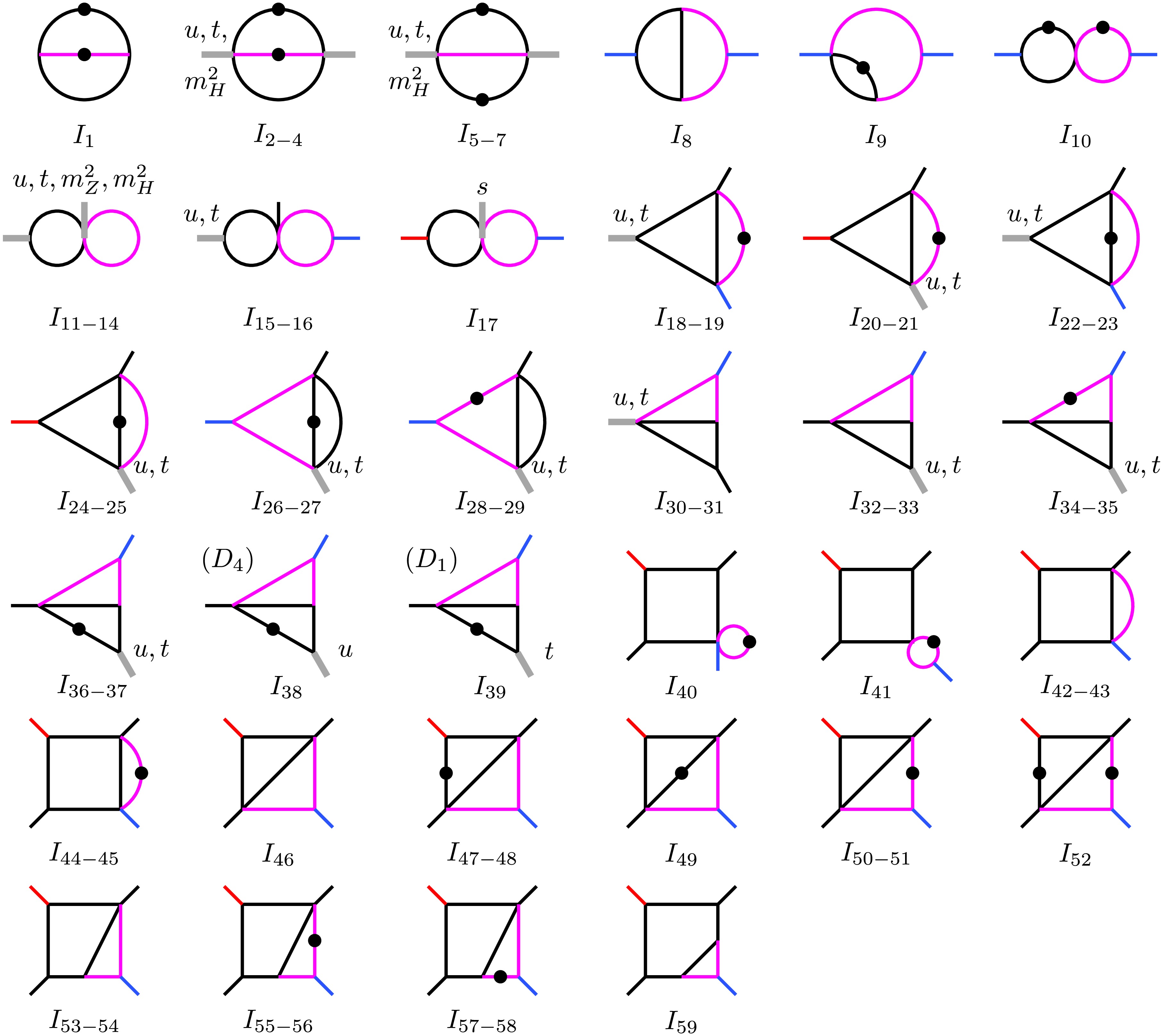
Figure 4. (color online) Same as Fig. 2, but for
$ {\cal{B}}_{2} $ .The canonical basis, constructed via the Magnus transformation, is given explicitly by
$ \begin{array}{*{20}{l}} \begin{split} g_{1} &= f_{1}\,, \qquad & g_{2} &= x\, f_{2}\,, \qquad & g_{3} &= y\, f_{3}\,, \qquad & g_{4} &= w\, f_{4}\,, \\ g_{5} &= 2\, f_{2}+(1+x)\, f_{5}\,, \qquad & g_{6} &= 2\, f_{3}+(1+y)\, f_{6}\,, \qquad & g_{7} &= 2\, f_{4}+(1+w)\, f_{7}\,, \qquad & g_{8} &= w\, f_{8}\,, \\ g_{9} &= r_{1} / (4 + w)\, { \sum\nolimits_{i} \beta_{9,i}\, f_{i}}\,, \qquad & g_{10} &= w r_{1}\, f_{10}\,, \qquad & g_{11} &= x\, f_{11}\,, \qquad & g_{12} &= y\, f_{12}\,, \\ g_{13} &= z\, f_{13}\,, \qquad & g_{14} &= w\, f_{14}\,, \qquad & g_{15} &= x r_{1}\, f_{15}\,, \qquad & g_{16} &= y r_{1}\, f_{16}\,, \\ g_{17} &= z r_{1}\, f_{17}\,, \qquad & g_{18} &= (x-w)\, f_{18}\,, \qquad & g_{19} &= (y-w)\, f_{19}\,, \qquad & g_{20} &= (x-z)\, f_{20}\,, \\ g_{21} &= (y-z)\, f_{21}\,, \qquad & g_{22} &= (x-w)\, f_{22}\,, \qquad & g_{23} &= (y-w)\, f_{23}\,, \qquad & g_{24} &= (x-z)\, f_{24}\,, \\ g_{25} &= (y-z)\, f_{25}\,, \qquad & g_{26} &= (x-w)\, f_{26}\,, \qquad & g_{27} &= (y-w)\, f_{27}\,, \qquad & g_{28} &= r_{1} / w\, { \sum\nolimits_{i} \beta_{28,i}\, f_{i}}\,, \\ g_{29} &= r_{1} / w\, { \sum\nolimits_{i} \beta_{29,i}\, f_{i}}\,, \qquad & g_{30} &= (x-w)\, f_{30}\,, \qquad & g_{31} &= (y-w)\, f_{31}\,, \qquad & g_{32} &= (x-w)\, f_{32}\,, \\ g_{33} &= (y-w)\, f_{33}\,, \qquad & g_{34} &= (x-w)\, r_{1}\, f_{34}\,, \qquad & g_{35} &= (y-w)\, r_{1}\, f_{35}\,, \qquad & g_{36} &= x\, (x-w)\, f_{36}\,, \\ g_{37} &= y\, (y-w)\, f_{37}\,, \qquad & g_{38} &= 2 w\, f_{32}-x\, f_{38}\,, \qquad & g_{39} &= 2 w\, f_{33}-y\, f_{39}\,, \qquad & g_{40} &= (x y-z w)\, f_{40}\,, \\ g_{41} &= (x y-z w)\, r_{1}\, f_{41}\,, \qquad & g_{42} &= (x-z)\, ( f_{42} - f_{44} )\,, \qquad & g_{43} &= (y-z)\, ( f_{43} - f_{45} )\,, \qquad & g_{44} &= (x y-z w)\, f_{44}\,, \\ g_{45} &= (x y-z w)\, f_{45}\,, \qquad & g_{46} &= r_{2}\, f_{46}\,, \qquad & g_{47} &= z\, (y-w)\, f_{47}\,, \qquad & g_{48} &= z\, (x-w)\, f_{48}\,, \\ g_{49} &= r_{3}\, f_{49}\,, \qquad & g_{50} &= r_{4}\, [\, f_{50} + f_{51} / (1+\mathbb{W}) \,]\,, \qquad & g_{51} &= r_{5}\, [\, f_{50} / (1+\mathbb{W}) + f_{51} \,]\,, \\ g_{52} &= 1 / w\, { \sum\nolimits_{i} \beta_{52,i}\, f_{i}}\,, \qquad & g_{53} &= x\, (y-w)\, f_{53}\,, \qquad & g_{54} &= y\, (x-w)\, f_{54}\,, \end{split}\\ g_{55} { {} = r_{1}\, [\, 2\, (x-z)\, f_{53} + (x-z+x y - z w)\, f_{55} + (x-z)\, f_{57} \,]\,, } \\ g_{56} { {} = r_{1}\, [\, 2\, (y-z)\, f_{54} + (y-z+x y - z w)\, f_{56} + (y-z)\, f_{58} \,]\,, } \\ g_{57} { {} = 2 w\, (x-z)\, f_{53} + [\, w\, (x-z) + (2+w)\, (x y - z w) \,]\, f_{55} + [\, x\, (y-w) + (x y - z w) \,]\, f_{57}\,, } \\ g_{58} { {} = 2 w\, (y-z)\, f_{54} + [\, w\, (y-z) + (2+w)\, (x y - z w) \,]\, f_{56} + [\, y\, (x-w) + (x y - z w) \,]\, f_{58}\,, } \\ g_{59} { {} = w\, [\, (x-z)\, f_{53} + (y-z)\, f_{54} + (x y-z w)\, f_{59} \,]\,, } \end{array} $
(40) with the non-vanishing coefficients
$ \beta_{i,j} $ provided in Appendix A. The five square roots,$ r_{1-5} $ , that appear in the canonical basis are given by$ \begin{aligned}[b] & r_1^2 = w\, (4 + w)\,, && r_4^2 = \lambda({\mathbb{W}} - x,\, {\mathbb{W}} z,\, {\mathbb{W}} + y + {\mathbb{W}} y)\,, \\ & r_2^2 = \lambda(z,\, w,\, z + w - x - y)\,, && r_5^2 = \lambda({\mathbb{W}} - y,\, {\mathbb{W}} z,\, {\mathbb{W}} + x + {\mathbb{W}} x)\,, \\ &r_3^2 = \lambda(1 + x - z,\, 1 + y - z,\, z w - x y)\,, &&\\[-20pt] \end{aligned} $
(41) where
$ {\mathbb{W}} $ is defined in Eq. (33). Notably,$ r_4 $ and$ r_5 $ are both nested square roots involving$ \vec{x} $ , indicating that the$ {\cal{B}}_2 $ branch exhibits a more intricate structure than the$ {\cal{B}}_1 $ branch. The differential one-form matrix for the canonical basis is constructed as described in Eq. (14), yielding an alphabet consisting of$ 26 $ even and$ 27 $ odd letters,● even letters
$ \begin{aligned}[b] \omega_{1} &= x\,, &\omega_{8} &= 4+w\,, &\omega_{15} &= 1-x+w\,, &\omega_{22} &= y^{2}-w\,(1+y)\,, \\ \omega_{2} &= y\,, & \omega_{9} &= x-z\,, &\omega_{16} &= 1-y+w\,, & \omega_{23} &= x\,(1+y) - z\,(1+w)\,, \\ \omega_{3} &= z\,, &\omega_{10} &= y-z\,, & \omega_{17} &= x+y-z-w\,, & \omega_{24} &= y\,(1+x) - z\,(1+w)\,, \\ \omega_{4} &= w\,, & \omega_{11} &= x-w\,, & \omega_{18} &= x y-z w\,,& \omega_{25} &= w\, (x-z)^2 - x\, (y-w)\, (xy-zw)\,, \\ \omega_{5} &= 1+x\,,\quad & \omega_{12} &= y-w\,, &\omega_{19} &= r_{2}^{2}\,,& \omega_{26} &= w\, (y-z)^2 - y\, (x-w)\, (xy-zw)\,. \\ \omega_{6} &= 1+y\,, & \omega_{13} &= 1+x-z\,, & \omega_{20} &= r_{3}^{2}\,, \\ \omega_{7} &= 1+w\,, & \omega_{14} &= 1+y-z\,,\quad &\omega_{21} &= x^{2}-w\,(1+x)\,, \end{aligned} $
(42) ● odd letters
$ \begin{aligned}[b] \omega_{27} &= \frac{w + r_{1}}{w - r_{1}} , & \omega_{41} &= \frac{x + y + {\mathbb{W}} (y - z) + r_{4}}{x + y + {\mathbb{W}} (y - z) - r_{4}}, \\ \omega_{28} &= \frac{2 x - w + r_{1}}{2 x - w - r_{1}}, & \omega_{42} &= \frac{x - y - {\mathbb{W}} (y - z) + r_{4}}{x - y - {\mathbb{W}} (y - z) - r_{4}}, \\ \omega_{29} &= \frac{2 y - w + r_{1}}{2 y - w - r_{1}}, & \omega_{43} &= \frac{x + y - 2 z + {\mathbb{W}} (y - z) + r_{4}}{x + y - 2 z + {\mathbb{W}} (y - z) - r_{4}}, \\ \omega_{30} &= \frac{2 (xy - zw) - (x - z) (w - r_1)}{2 (xy - zw) - (x - z) (w + r_1)}, & \omega_{44} &= \frac{x + y + {\mathbb{W}} (x + z) + r_{5}}{x + y + {\mathbb{W}} (x + z) - r_{5}}, \\ \omega_{31} &= \frac{2 (xy - zw) - (y - z) (w - r_1)}{2 (xy - zw) - (y - z) (w + r_1)}, & \omega_{45} &= \frac{x + y + {\mathbb{W}} (x - z) + r_{5}}{x + y + {\mathbb{W}} (x - z) - r_{5}}, \\ \omega_{32} &= \frac{x + y + r_{2}}{x + y - r_{2}}, & \omega_{46} &= \frac{y - x - {\mathbb{W}} (x - z) + r_{5}}{y - x - {\mathbb{W}} (x - z) - r_{5}}, \\ \omega_{33} &= \frac{x - y + r_{2}}{x - y - r_{2}}, & \omega_{47} &= \frac{x + y - 2 z + {\mathbb{W}} (x - z) + r_{5}}{x + y - 2 z + {\mathbb{W}} (x - z) - r_{5}}, \\ \omega_{34} &= \frac{x + y - 2 z + r_{2}}{x + y - 2 z - r_{2}}, & \omega_{48} &= \frac{\xi_{1} + r_{1} r_{3}}{\xi_{1} - r_{1} r_{3}}, \\ \omega_{35} &= \frac{x - y - x y + z w + r_{3}}{x - y - x y + z w - r_{3}}, & \omega_{49} &= \frac{\xi_{2} + (1 + {\mathbb{W}}) r_{2} r_{4}}{\xi_{2} - (1 + {\mathbb{W}}) r_{2} r_{4}}, \\ \omega_{36} &= \frac{y - x - x y + z w + r_{3}}{y - x - x y + z w - r_{3}}, & \omega_{50} &= \frac{\xi_{3} + (1 + {\mathbb{W}}) r_{2} r_{5}}{\xi_{3} - (1 + {\mathbb{W}}) r_{2} r_{5}}, \\ \omega_{37} &= \frac{x + y + x y - z (2 + w) + r_{3}}{x + y + x y - z (2 + w) - r_{3}}, & \omega_{51} &= \frac{\xi_{4} + (1 + {\mathbb{W}}) r_{3} r_{4}}{\xi_{4} - (1 + \mathbb{W}) r_{3} r_{4}}, \\ \omega_{38} &= \frac{x + y + x y - z (2 x - w) + r_{3}}{x + y + x y - z (2 x - w) - r_{3}}, & \omega_{52} &= \frac{\xi_{5} + (1 + {\mathbb{W}}) r_{3} r_{5}}{\xi_{5} - (1 + {\mathbb{W}}) r_{3} r_{5}}, \\ \omega_{39} &= \frac{x + y + x y - z (2 y - w) + r_{3}}{x + y + x y - z (2 y - w) - r_{3}}, & \omega_{53} &= \frac{\xi_{6} + r_{4} r_{5}}{\xi_{6} - r_{4} r_{5}}, \\ \omega_{40} &= \frac{x + y + {\mathbb{W}} (y + z) + r_{4}}{x + y + {\mathbb{W}} (y + z) - r_{4}}, \\[-10pt] \end{aligned} $
(43) where the explicit expressions for
$ \xi_i\; (i = 1, \ldots, 6) $ are given in Appendix A.In the
$ {\cal{B}}_2 $ branch, although the alphabet contains five radicals, the canonical MIs exhibit only three distinct radical structures. They can therefore be classified into three disjoint subsets, as summarized in Table 2. The MIs in$ S_{2\,(00000)} $ , as well as those in$ S_{2\,(10000)} $ after applying the rationalization transformation$ \Phi_1 $ , can both be expressed in terms of GPLs. In contrast, a GPL representation of the MIs in$ S_{2\,(11111)} $ would require the simultaneous rationalization of all five radicals, which is impractical. However, at lower orders of the$ \epsilon $ -expansion, the radical structure of a canonical MI is relatively simple, and the radical index has not yet reached its maximum value. At$ {\cal{O}}(\epsilon) $ , the only non-vanishing MI in$ S_{2\,(11111)} $ is$ g_{52} $ , which is independent of all five radicals. The radical indices of the MIs in$ S_{2\,(11111)} $ at the second, third, and fourth orders in$ \epsilon $ are listed in detail in Table 3.Subset Radical structure Master integrals ( $ \boldsymbol{g_i} $ )Count $ S_{2\,(00000)} $ $ \{\;\} $ 1−7, 11−14, 18−25, 40, 42−45 24 $ S_{2\,(10000)} $ $ \{r_1\} $ 8−10, 15−17, 26−39, 41 21 $ S_{2\,(11111)} $ $ \{r_1, r_2, r_3, r_4, r_5\} $ 46−59 14 Table 2. Same as Table 1, but for
$ {\cal{B}}_2 $ .Radical index Master integrals ( $ \boldsymbol{g_i} $ )$ \epsilon^2 $ $ \epsilon^3 $ $ \epsilon^4 $ $ (00000) $ 46,50,51,53,54,59 46 $ (10000) $ 47,48,52,55−58 53,54,59 $ (10100) $ 49 47−49,52,55−58 53,54,59 $ (10110) $ 50 $ (10101) $ 51 $ (10111) $ 47−52,55−58 $ (11111) $ 46 Table 3. Radical indices of the MIs in
$ S_{2\,(11111)} $ up to$ {\cal{O}}(\epsilon^4) $ .At
$ {\cal{O}}(\epsilon^2) $ , the MIs in$ S_{2\,(11111)} $ involve at most two radicals,$ r_1 $ and$ r_3 $ . The radical structure of$ S_{2\,(11111)} $ at this order closely parallels that of the$ {\cal{B}}_{1\,(11)} $ subsystem in the$ {\cal{B}}_1 $ branch:System Radicals $ S_{2 { (11111) }}\ \text{at}\ \mathcal{O}\left(\epsilon^2\right)$ $\sqrt{w(4+w)} $ $ \sqrt{\lambda(1+x-z, 1+y-z, z w-x y)}$ $\mathcal{B}_{1(11)} $ $\sqrt{w(4+w)} $ $\sqrt{\lambda(x, z, w)} $ all radicals are square roots, with radicands given by Källén-type functions. Motivated by this structural similarity, we construct a variable transformation—analogous to Ψ—that simultaneously rationalizes
$r_1$ and$r_3$ :$ \Lambda(x, z, w) = \Phi_1(w) \,\circ\, \Phi_2(1+x-z, 1+y-z; \,zw-xy)\,. $
(44) Explicitly, this transformation reads
$ \left\lbrace\, \begin{aligned} & x = \frac{(1 + {\mathbb{W}})\,y + {\mathbb{W}}^2 \big[\, ({\mathbb{X}} - {\mathbb{Z}}) + {\mathbb{X}}y\, (1 - {\mathbb{Z}}) \,\big]}{(1 + {\mathbb{W}}) \big[\, 1 + y\,({\mathbb{X}} - {\mathbb{Z}}) \,\big] + {\mathbb{W}}^2 {\mathbb{Z}}\, (1 - {\mathbb{X}})}, \\ & z = \frac{(1 + {\mathbb{W}})\,(1 + {\mathbb{X}}y)\, \big[\, 1 + y\,(1 - {\mathbb{Z}}) \,\big]}{(1 + {\mathbb{W}}) \big[\, 1 + y\,({\mathbb{X}} - {\mathbb{Z}}) \,\big] + {\mathbb{W}}^2{\mathbb{Z}}\, (1 - {\mathbb{X}})}, \\ & w = \frac{{\mathbb{W}}^2}{1+{\mathbb{W}}}, \end{aligned} \right.\, $
(45) under which
$ r_1 $ takes the same form as in Eq. (36), and$ r_3 $ admits the following rationalized expression in terms of$ ({\mathbb{X}}, y, {\mathbb{Z}}, {\mathbb{W}}) $ :$ r_3 = \frac{({\mathbb{W}} - y)\, (1 - {\mathbb{X}} - {\mathbb{Z}})\, (y + {\mathbb{W}} + y {\mathbb{W}})}{(1 + {\mathbb{W}}) \big[\, 1 + y\,({\mathbb{X}} - {\mathbb{Z}}) \,\big] + {\mathbb{W}}^2 {\mathbb{Z}}\, (1 - {\mathbb{X}})}\,. $
(46) Consequently, the integrals listed in the first three rows of Table 3, including all
$ {\cal{O}}(\epsilon^2) $ MIs in$ S_{2\,(11111)} $ , can be expressed in terms of GPLs.As shown in the dashed box of Table 3, at the third and fourth orders in the
$ \epsilon $ -expansion, some MIs in$ S_{2\,(11111)} $ exhibit more intricate radical structures with radical indices exceeding$ (10100) $ , including$ \{r_1,r_3,r_4\} $ ,$ \{r_1,r_3,r_5\} $ ,$ \{r_1,r_3,r_4,r_5\} $ , and$ \{r_1,r_2,r_3,r_4,r_5\} $ . At present, however, no transformations are known that can rationalize these more involved radical structures, owing to the nested square roots$ r_4 $ and$ r_5 $ . Nevertheless, by virtue of the first-order recursion relation and the associated second-order relation obtained via integration by parts,$ \begin{aligned}[b] \vec{g}^{\,(p)}(\vec{x}) =& \int_{\gamma} {\rm d}\mathbb{A}\, \vec{g}^{\,(p-1)} + \vec{g}^{\,(p)}(\vec{x}_0)\,, \\ \vec{g}^{\,(p)}(\vec{x}) =& \int_{\gamma} \big[\, \mathbb{A}(\vec{x}) - \mathbb{A} \,\big]\, {\rm d}\mathbb{A}\, \vec{g}^{\,(p-2)}\\ &+ \big[\, \mathbb{A}(\vec{x}) - \mathbb{A}(\vec{x}_0) \,\big]\, \vec{g}^{\,(p-1)}(\vec{x}_0) + \vec{g}^{\,(p)}(\vec{x}_0)\,, \end{aligned} $
(47) the integrals in the dashed box can be systematically reduced and ultimately expressed as one-fold integrals over GPLs.
For the
$ {\cal{B}}_2 $ branch, the boundary conditions used to fix the integration constants of the MIs are as follows:● permutation symmetries (28)
Master integrals that share the same topological structure are related by permutation symmetries of the external kinematic invariants, as exemplified by
$ g_{18-21} $ . Figure 4 shows that the$ 59 $ MIs in$ {\cal{B}}_2 $ reduce to$ 31 $ independent topologies, yielding$ 28 $ homogeneous boundary conditions induced by these permutation symmetries.● common topologies with
$ {\cal{B}}_1 $ (16)Among the
$ 31 $ independent topologies in$ {\cal{B}}_2 $ ,$ 16 $ coincide with those in$ {\cal{B}}_1 $ , while the remaining$ 15 $ are fixed by the boundary conditions below.●
$ \mathrm{HyperInt} $ evaluation (4)The integrals
$ g_{22,40,42,44} $ , which belong to the subset$ S_{2\, (00000)} $ , are evaluated analytically using the$ \mathrm{HyperInt} $ package [62].● vanishing conditions (11)
$ g_{38,41,46,47,49,50,52,53,55,57,59} $ vanish at$ (x,y,z,w)=(0,0,1,0) $ .The explicit expressions for all
$ 59 $ canonical MIs in$ {\cal{B}}_2 $ up to$ {\cal{O}}(\epsilon^2) $ are collected in Appendix C. The complete analytic expressions up to$ {\cal{O}}(\epsilon^4) $ are provided in the supplementary file$ \mathrm{B2.m} $ . -
As discussed in Sec. II, the topologies associated with the
$ ZZH $ vertex are obtained from the four topologies in Fig. 1 by replacing the W propagator with a Z propagator. Among these, the two family branches induced by the planar topologies are denoted by$ {\cal{C}}_1 $ and$ {\cal{C}}_2 $ , respectively. For the$ 62 $ MIs in the$ {\cal{B}}_1 $ branch associated with the$ WWH $ vertex, all integrals remain finite in the limit$ m_W^2 \rightarrow m_Z^2 $ (i.e.,$ z \rightarrow -1 $ ), with the exception of$ g_{9} $ ,$ g_{13} $ , and$ g_{51} $ . Moreover, the singular parts of these three integrals are not independent but satisfy the proportionality relation$ \breve{g}_9 \,:\, \breve{g}_{13} \,:\, \breve{g}_{51} = 1 \,:\, 2 \,:\, -1\,, $
(48) where
$ \breve{g} $ denotes the singular part of g in the limit$ z \rightarrow -1 $ . This indicates that the$ {\cal{B}}_1 $ branch contains only one linearly independent divergence. Accordingly, the canonical MIs for the$ {\cal{B}}_1 $ branch with the simplest divergent structure can be chosen as$ E = E_{r} \cup E_s = \big\{ g_{i \neq 9,13,51},\; 2 g_9 - g_{13},\; g_9+g_{51} \big\} \cup \big\{ g_9 \big\}\,. $
(49) The MIs in the set
$ E_r $ are regular in the limit$ z \rightarrow -1 $ , whereas$ E_s $ contains the only divergent MI. This implies that the$ {\cal{C}}_1 $ branch associated with the$ ZZH $ vertex contains$ 61 $ independent MIs, and a canonical basis can be constructed as$ \vec{h} = \lim\limits_{z \rightarrow -1}\,\left( g_{i\neq 9,13,51},\; 2g_9 - g_{13},\; g_9 + g_{51} \right)\,, $
(50) which have been verified through the IBP reduction using
$ \mathrm{Kira} $ . Specifically, the analytic expressions for$ h_{60} $ and$ h_{61} $ up to$ {\cal{O}}(\epsilon^2) $ are given as follows:$ \begin{aligned}[b] h_{60} ={}& \lim_{z \rightarrow -1}\,(2g_9 - g_{13}) = 1+\epsilon^{2}\,\pi^2/6 \,, \\ h_{61} ={}& \lim_{z \rightarrow -1}\,(g_{9} + g_{51}) = \epsilon\, [\, G(a_3;y) + G(a_{22};\mathbb{X}) \,] + \epsilon^2\, \big\{ 4 G(a_3;y)\, [\, G(a_{24};\mathbb{X}) - G(a_{26};\mathbb{X}) \,] \\ & - 2G(a_3;\mathbb{W})\, [\, G(a_{8};y) - G(a_{12};\mathbb{X}) + G(a_{12};\mathbb{Z}) + G(a_{14};\mathbb{X}) - G(a_{14};\mathbb{Z}) - G(a_{15};y) \,] \\ & + G(a_{16};\mathbb{Z})\, [\, G(a_2;\mathbb{X}) - 2 G(a_{12};\mathbb{X}) - 2 G(a_{14};\mathbb{X}) - 4 G(a_{24};\mathbb{X}) + 4 G(a_{26};\mathbb{X}) \,] \\ & + G(a_1,a_{16};\mathbb{Z}) + 4 G(a_1,a_{22};\mathbb{X}) + G(a_2,a_{23};\mathbb{X}) - 4 G(a_3,a_3;y)+ 2 G(a_8,a_3;y) \\ & - 2 G(a_{12},a_{16};\mathbb{Z}) + 2 G(a_{12},a_{22};\mathbb{X}) - 2 G(a_{12},a_{23};\mathbb{X}) - 2 G(a_{14},a_{16};\mathbb{Z}) \\ & + 2 G(a_{14},a_{22};\mathbb{X}) - 2 G(a_{14},a_{23};\mathbb{X}) + 2 G(a_{15},a_3;y) - 4 G(a_{22},a_{22};\mathbb{X}) \\ &- 4 G(a_{24},a_{23};\mathbb{X}) - 4 G(a_{26},a_{22};\mathbb{X}) + 4G(a_{26},a_{23};\mathbb{X}) \big\}\,, \end{aligned} $
(51) where the weights
$ a_i $ are defined in Eq. (B2), and the variables$ {\mathbb{X}} $ ,$ {\mathbb{Z}} $ , and$ {\mathbb{W}} $ satisfy the constraint$ {\mathbb{Z}}\,({\mathbb{X}}-1)\,\frac{{\mathbb{W}}^2}{1 + {\mathbb{W}}}=1\,. $
(52) The analytic expressions up to
$ {\cal{O}}(\epsilon^4) $ are provided in the supplementary file$ \mathrm{C1.m} $ . For the$ {\cal{B}}_2 $ branch associated with the$ WWH $ vertex, all MIs are regular in the limit$ z \rightarrow -1 $ . Consequently, the$ {\cal{C}}_2 $ branch associated with the$ ZZH $ vertex contains$ 59 $ independent MIs, and a canonical basis can be conveniently chosen as$ \vec{h}=(g_{1},\ldots,g_{59})\,|_{z\,=\,-1}\,, $
(53) which can also be verified using
$ \mathrm{Kira} $ .In summary, we derive analytic expressions for the canonical MIs in the four branches associated with the four planar topologies. Most of these MIs can be expressed in terms of GPLs, while a subset is represented, at
$ {\cal{O}}(\epsilon^3) $ and$ {\cal{O}}(\epsilon^4) $ , by one-fold integrals over GPLs. To verify the correctness of our analytic expressions for the MIs, we cross-check them against independent numerical results obtained using$ \mathrm{AMFlow} $ [63]. The GPLs are evaluated using the$ \mathrm{NumPolyLog} $ [64, 65] package, and the one-fold integrals over GPLs are computed with the built-in$ \mathrm{NIntegrate} $ function in$ \mathrm{Mathematica} $ . The numerical check is performed at a benchmark point in the Euclidean region,$ (s, t, u, m_Z^2, m_H^2, m_W^2) = (-11/9,\, -1/15,\, -1/6,\, -19/18,\, -2/5, 1)\,, $
(54) and the results for representative MIs are summarized in Table 4. These integrals are selected to capture the main nontrivial structures arising in our calculation:
$ g_{62} $ exhibits the most intricate radical structure in the$ {\cal{B}}_1 $ branch;$ g_{52} $ serves as a representative MI in the$ {\cal{B}}_2 $ branch, admitting a one-fold integral representation; and$ h_{61} $ is obtained from$ g_9 + g_{51} $ in the$ {\cal{B}}_1 $ branch by taking the limit$ z \rightarrow -1 $ , as shown in Eq. (50). The numerical results obtained from our analytic expressions show excellent agreement with those computed using the auxiliary mass flow method, with full consistency at the level of$ 30 $ significant digits.Integral Method Numerical result $ g_{62} \in {\cal{B}}_1 $ Analytic $ \begin{aligned} -\,&0.664957668643736033610081193355\,\epsilon^3\\-\,&4.726392850105022560752360395509\,\epsilon^4 \end{aligned} $ $ \mathrm{AMFlow} $ $ \begin{aligned} -\,&0.664957668643736033610081193355\,\epsilon^3\\-\,&4.726392850105022560752360395509\,\epsilon^4 \end{aligned} $ $ g_{52} \in {\cal{B}}_2 $ Analytic $ \begin{aligned}&0.064538521137571171672923915684\,\epsilon\\+\,&0.330242367516912611342417320261\,\epsilon^2\\+\,&0.708117837983710638396022672956\,\epsilon^3\\+\,&1.099406021270770791529184043986\,\epsilon^4 \end{aligned} $ $ \mathrm{AMFlow} $ $ \begin{aligned}&0.064538521137571171672923915684\,\epsilon\\+\,&0.330242367516912611342417320261\,\epsilon^2\\+\,&0.708117837983710638396022672956\,\epsilon^3\\+\,&1.099406021270770791529184043986\,\epsilon^4 \end{aligned} $ $ h_{61} \in {\cal{C}}_1 $ Analytic $ \begin{aligned}&0.863046217355342782317657017981\,\epsilon\\+\,&7.990926766799493648452542524898\,\epsilon^2\\+\,&28.96621761952415138613880610204\,\epsilon^3\\+\,&122.0034204649560223899898864194\,\epsilon^4 \end{aligned} $ $ \mathrm{AMFlow} $ $ \begin{aligned}&0.863046217355342782317657017981\,\epsilon\\+\,&7.990926766799493648452542524898\,\epsilon^2\\+\,&28.96621761952415138613880610204\,\epsilon^3\\+\,&122.0034204649560223899898864194\,\epsilon^4 \end{aligned} $ Table 4. Numerical comparison of the analytic expressions with the corresponding
$ \mathrm{AMFlow} $ results for three representative MIs. The tabulated values from the two methods agree to$ 30 $ significant digits. -
To apply our analytic results to the calculation of the
$ gg \rightarrow ZH $ cross section, the expressions derived in the Euclidean region must be analytically continued to the physical region. In the following, we use the$ {\cal{B}}_1 $ branch as a representative example to illustrate the analytic continuation procedure and to validate the continued results at several benchmark points. For the partonic process$ gg \rightarrow ZH $ , the physical region is defined by$ \begin{aligned}[b] s >& (m_Z + m_H)^2\,, \\ \frac{m_Z^2 + m_H^2 - s - \sqrt{\lambda(s,m_Z^2,m_H^2)}}{2} \leqslant t \leqslant & \frac{m_Z^2 + m_H^2 - s + \sqrt{\lambda(s,m_Z^2,m_H^2)}}{2}\,. \end{aligned} $
(55) The analytic continuation to the physical region is determined by the Feynman
$ {\rm i} 0^+ $ prescription. Following this prescription, we assign infinitesimal imaginary parts to the external kinematic scales and to the internal mass squared as follows:$ s + {\rm i} 0^+\,, \quad t + {\rm i} 0^+\,, \quad m_Z^2 + {\rm i} 0^+\,, \quad m_H^2 + {\rm i} 0^+\,, \quad m_W^2 - {\rm i} 0^+\,. $
(56) The corresponding prescription for the dimensionless variables is then given by
$ x - {\rm i}0^+\,, \qquad y - {\rm i}0^+\,, \qquad z - {\rm i}0^+\,, \qquad w - {\rm i}0^+\,. $
(57) In principle, the Feynman prescription specified above uniquely determines the analytic continuation of the MIs to the physical region. However, because the solution of the differential-equation system involves rationalizing transformations, the associated branch choices must be handled with care when performing the continuation. At
$ {\cal{O}}(\epsilon) $ , these transformations convert the$ {\rm d}\log $ forms in the coefficient matrices into linear combinations of$ {\rm d}\log $ forms expressed in the rationalized variables. After integration, they yield the corresponding weight-one GPLs, i.e., logarithms. In the Euclidean region, this rewriting of logarithms typically does not introduce additional constant terms. In the physical region, however, one must verify that the resulting logarithmic combinations match the corresponding logarithms in the original variables, evaluated with the Feynman prescriptions specified above. For generic nonzero complex quantities a and b, one has$ \begin{aligned}[b] \log(ab) =& \log a+\log b + 2 \pi {\rm i} \Big[ \Theta(-{\rm{Im}} \;a)\, \Theta(-{\rm{Im}} \;b)\, \Theta({\rm{Im}} \;ab) \\ &-\Theta({\rm{Im}} \;a)\, \Theta({\rm{Im}} \;b)\, \Theta(-{\rm{Im}} \;ab) \Big]\,. \end{aligned} $
(58) Consequently, in the physical region, the logarithmic combinations obtained after rationalization may differ from the corresponding logarithms expressed in the original variables by integer multiples of
$ 2\pi {\rm i} $ . We refer to the logarithms in the original variables at$ {\cal{O}}(\epsilon) $ as first-entry logarithms. By the first-entry condition, discontinuities of the MIs can arise only from these first-entry logarithms [66, 67]. It is therefore sufficient to check whether the weight-one GPL combinations obtained after the rationalizing transformations match the corresponding first-entry logarithms in the original variables. When evaluating the analytic expressions in the physical region, the required constant corrections are included accordingly. These constant corrections are propagated order by order to higher weights through the iterative solution of the differential equations, and no additional independent corrections are required for the higher-weight GPLs [68].Table 5 summarizes the nine first-entry logarithms that appear at
$ {\cal{O}}(\epsilon) $ and, for each, lists the MIs whose$ {\cal{O}}(\epsilon) $ coefficients involve that logarithm, grouped by radical index. As discussed above, when a first-entry logarithm is expressed in terms of GPLs after the corresponding rationalizing transformation, the correction term needed for the resulting GPL expression can be obtained by applying Eq. (58). With the Feynman prescriptions specified above, we find that such corrections are needed only for$ \log(1+z) $ and$ \log(1+w) $ after the relevant rationalizing transformations; for all other first-entry logarithms, no correction term arises. Accordingly, the entries for which the first-entry logarithms require corrections are marked by dashed boxes in Table 5. Among the nonempty boxed entries at weight one, the only MI is$ g_{51} $ , and the corresponding correction originates from the$ \log(1+z) $ term. Under the corresponding rationalizing transformation$ \Psi(x, z, w) $ , this logarithm is expressed asFirst-entry logarithm Master integrals by radical index $ (00) $ $ (10) $ $ (01) $ $ (11) $ $ \log x $ 2 48, 52 $ \log y $ 3 48, 53 $ \log z $ 4 48, 53 $ \log w $ 5 48 $ \log(1+x) $ 7, 11 29 51 $ \log(1+y) $ 8, 12 52, 54 51, 58 $ \log(1+z) $ 9, 13 51 $ \log(1+w) $ 10, 14 28 $ \log\big[(w+r_1)/(w-r_1)\big] $ 6, 16-19, 32 33, 49, 60 Table 5.
$ {\cal{O}}(\epsilon) $ MIs in the$ {\cal{B}}_1 $ branch involving first-entry logarithms, classified by radical index.$ \begin{aligned}[b] \log(1+z) &= G(a_{16};{\mathbb{Z}})+G(a_{23};{\mathbb{X}})-2\pi {\rm i}\Bigl\{\Theta\bigl[-\lambda(x,z,w)\bigr]\,\Theta(-1-z)\,\Theta(-x-z-w) \\ &\quad+\Theta\bigl[\lambda(x,z,w)\bigr]\,\Theta\bigl[w\,({\mathbb{X}}{\mathbb{Z}}-1)\bigr]\,\Theta\bigl[(1-{\mathbb{X}})^2\,\bigl(w{\mathbb{X}}+z(1+z)\bigr)+z^2\,{\mathbb{X}}\bigr]\Bigr\}\,. \end{aligned} $
(59) The
$ \log(1+w) $ correction appears in a slightly different manner. For$ g_{10} $ and$ g_{14} $ , whose radical index is$ (00) $ , the corresponding differential-equation subsystems can be solved directly in terms of GPLs without requiring any rationalizing transformation. Consequently, no correction term is needed for their$ \log(1+w) $ contributions. However, the same MIs may also occur as nodes in tropical trees with nonzero radical indices. For example, in the trees rooted at$ g_{15} $ ,$ g_{16} $ , and$ g_{34} $ , which carry radical index$ (10) $ , the relevant$ \log(1+w) $ term is instead expressed in terms of GPLs after applying the rationalizing transformation$ \Phi_1(w) $ , yielding$ \log(1+w) = G(a_5;{\mathbb{W}})+G(a_6;{\mathbb{W}})-G(-1;{\mathbb{W}}) -2\pi {\rm i}\,\Theta(-1-w)\,. $
(60) To validate our analytic continuation procedure, we consider two representative examples:
$ g_{51} $ in the tropical-tree subsystem rooted at$ g_{51} $ , and$ g_{10} $ in a tropical-tree subsystem with radical index$ (10) $ . We explicitly present their analytic expressions at$ {\cal{O}}(\epsilon) $ , including the required$ 2\pi i $ correction terms, and verify their numerical agreement with$ \mathrm{AMFlow} $ up to$ {\cal{O}}(\epsilon^4) $ . For$ g_{51} $ , we evaluate the analytic expression at two benchmark points, referred to as point 1 and point 2:$ \begin{aligned} {\rm{point}}\ 1:\quad (x,y,z,w)&=(-29/4,\, 7/4,\, -9/7,\, -17/7)\,, \\ {\rm{point}}\ 2:\quad (x,y,z,w)&=(-13/10,\, 19/15,\, -44/43,\, -17/7)\,. \end{aligned} $
(61) Here, point 1 is a physical-region point near the production threshold, satisfying
$ \biggl| \frac{x + \left( \sqrt{-z} + \sqrt{-w} \right)^2}{x} | \simeq 2 \times 10^{-4}\,, $
(62) with z and w chosen as simple rational values close to the corresponding physical mass ratios. Point 2 is instead chosen near the pseudo-threshold
$ z = -1 $ . After applying the corresponding rationalizing transformation, the$ {\cal{O}}(\epsilon) $ coefficient of$ g_{51} $ is given below, with the relevant constant correction indicated explicitly:$ {\includegraphics[width=0.8\paperwidth]{CPC-2026-0321-Eq.63.jpg}}$
(63) For
$ g_{10} $ , the numerical check is performed at points 1 and 3. The latter is chosen near the pseudo-threshold$ w = -1 $ and is defined by$ {\rm{point}}\ 3:\qquad (x,y,z,w)=(-23/5,\, 29/24,\, -9/7,\, -38/37)\,. $
(64) After applying the corresponding rationalizing transformation, the
$ {\cal{O}}(\epsilon) $ coefficient of$ g_{10} $ is given by$ {\includegraphics[width=0.8\paperwidth]{CPC-2026-0321-Eq.65.jpg}}$
(65) Table 6 lists the numerical values of these MIs computed from the analytic expressions, together with the corresponding results obtained using
$ \mathrm{AMFlow} $ . In all cases, the two sets of results agree to$ 30 $ significant digits.Integral Method Numerical result $ g_{10}\in{\cal{B}}_1 $ at point 1Analytic $ \begin{aligned}&(0.356674943938732378912638711241-3.141592653589793238462643383280\,i) \,\epsilon\\+\,&(17.05293534906933005662400858990+1.694564335468304064318952995781\,i)\,\epsilon^2\\+\,&(10.06238117392647773804413414918+42.64973557588196949033627002992\,i)\,\epsilon^3\\-\,&(56.56423615955873758893102073177-84.47126476234965253805448901920\,i)\,\epsilon^4 \end{aligned} $ $ \mathrm{AMFlow} $ $ \begin{aligned}&(0.356674943938732378912638711241-3.141592653589793238462643383280\,i)\,\epsilon\\+\,&(17.05293534906933005662400858990+1.694564335468304064318952995781\,i)\,\epsilon^2\\+\,&(10.06238117392647773804413414918+42.64973557588196949033627002992\,i)\,\epsilon^3\\-\,&(56.56423615955873758893102073177-84.47126476234965253805448901920\,i)\,\epsilon^4 \end{aligned} $ $ g_{10}\in{\cal{B}}_1 $ at point 3Analytic $ \begin{aligned} -\,&(3.610917912644224444368095671031+3.141592653589793238462643383280\,i)\,\epsilon\\-\,&(8.106325032238807717534575398018+45.45991351743298060529827089678\,i)\,\epsilon^2\\+\,&(114.7068013027885348196369729927-292.5675287057836410728435902073\,i)\,\epsilon^3\\+\,&(1321.012159448454915768761955509-981.8690843193124101827869503218\,i)\,\epsilon^4 \end{aligned} $ $ \mathrm{AMFlow} $ $ \begin{aligned} -\,&(3.610917912644224444368095671031+3.141592653589793238462643383280\,i)\,\epsilon\\-\,&(8.106325032238807717534575398018+45.45991351743298060529827089678\,i)\,\epsilon^2\\+\,&(114.7068013027885348196369729927-292.5675287057836410728435902073\,i)\,\epsilon^3\\+\,&(1321.012159448454915768761955509-981.8690843193124101827869503218\,i)\,\epsilon^4 \end{aligned} $ $ g_{51}\in{\cal{B}}_1 $ at point 1Analytic $ \begin{aligned}&\phantom{(}4.096945343922158051282654380570\,\epsilon\\-\,&(8.803716788142120881981264149685-27.83186832486123671600450766893\,i)\,\epsilon^2\\-\,&(114.8786140024535778364239393103-14.87613043969147173039118631646\,i)\,\epsilon^3\\-\,&(248.5706152088352565828306590787+216.5660933421071077429574631392\,i)\,\epsilon^4 \end{aligned} $ $ \mathrm{AMFlow} $ $ \begin{aligned}&\phantom{(}4.096945343922158051282654380570\,\epsilon\\-\,&(8.803716788142120881981264149685-27.83186832486123671600450766893\,i)\,\epsilon^2\\-\,&(114.8786140024535778364239393103-14.87613043969147173039118631646\,i)\,\epsilon^3\\-\,&(248.5706152088352565828306590787+216.5660933421071077429574631392\,i)\,\epsilon^4 \end{aligned} $ $ g_{51}\in{\cal{B}}_1 $ at point 2Analytic $ \begin{aligned}&\phantom{(}2.276925346213468063125613227844\,\epsilon\\+\,&(23.30607053594045226506026221897+27.54325773426026399896338828720\,i)\,\epsilon^2\\-\,&(5.852872209488398457556858569111-299.5649480027405921185976837404\,i)\,\epsilon^3\\-\,&(1075.442311348276408290179689446-1362.944600148010055075208057434\,i)\,\epsilon^4 \end{aligned} $ $ \mathrm{AMFlow} $ $ \begin{aligned}&\phantom{(}2.276925346213468063125613227844\,\epsilon\\+\,&(23.30607053594045226506026221897+27.54325773426026399896338828720\,i)\,\epsilon^2\\-\,&(5.852872209488398457556858569111-299.5649480027405921185976837404\,i)\,\epsilon^3\\-\,&(1075.442311348276408290179689446-1362.944600148010055075208057434\,i)\,\epsilon^4 \end{aligned} $ Table 6. Numerical check of the analytically continued expressions for
$ g_{10} $ and$ g_{51} $ against$ \mathrm{AMFlow} $ . The tabulated values from the two methods agree to$ 30 $ significant digits. -
The
$ gg \rightarrow ZH $ process is an important component of$ ZH $ production at the LHC, contributing approximately 10% to the total cross section and becoming increasingly significant in the boosted regime. In this work, we analytically compute the planar MIs for the two-loop NLO EW corrections to$ gg \rightarrow ZH $ arising from light-fermion loops. For the two family branches associated with the$ WWH $ vertex,$ {\cal{B}}_1 $ and$ {\cal{B}}_2 $ , we construct canonical bases using the Magnus-expansion method and derive analytic expressions for the MIs up to$ {\cal{O}}(\epsilon^4) $ via the canonical differential-equations method. In the$ {\cal{B}}_1 $ branch, only two square roots appear, and the MIs are classified into four subsets according to their radical structures. For the subsystems induced by these subsets, we apply rationalizing transformations separately, yielding relatively compact analytic expressions for the MIs in terms of GPLs. In the$ {\cal{B}}_2 $ branch, five nontrivial radicals appear that cannot be rationalized simultaneously, and the corresponding MIs are classified into three subsets. For the subset with the most intricate radical structure, certain MIs require their$ \epsilon^3 $ and$ \epsilon^4 $ expansions to be expressed as one-fold integrals over GPLs, while the remaining integrals can still be expressed in terms of GPLs. The canonical MIs for the two branches associated with the$ ZZH $ vertex can be derived analytically from their counterparts in the corresponding$ WWH $ vertex branches. We also discuss the analytic continuation of the MIs to the physical region, using the$ {\cal{B}}_1 $ branch as an illustrative example and identifying the necessary constant corrections from the first-entry logarithms. To validate our analytic expressions, we numerically evaluate the MIs at one Euclidean point and three representative non-Euclidean points near thresholds or pseudo-thresholds. The results are in perfect agreement with those obtained using$ \mathrm{AMFlow} $ .The analytic expressions for the MIs presented in this work provide essential input for future studies of the complete NLO EW corrections to
$ gg \rightarrow ZH $ . For the light-fermion-loop contribution considered here, the MIs associated with the remaining non-planar topologies must still be evaluated before the corresponding two-loop virtual amplitude can be constructed. Compared with the MIs evaluated in this work, these non-planar MIs are expected to be more challenging to compute analytically. The corresponding integral branches typically contain a larger number of MIs and may involve more complicated radical structures, or even more intricate algebraic structures. For the non-planar branch of the second integral family, a maximal-cut analysis of one of its sectors reveals that the associated algebraic curve is elliptic. This indicates that the analytic expressions for the corresponding MIs lie beyond the framework of multiple polylogarithms. The computation of these non-planar MIs, together with the subsequent construction of the corresponding two-loop virtual amplitude, is left for future work. -
The non-vanishing coefficients
$ \alpha_{i,j} $ in Eq. (21) are given as follows:$ \begin{aligned}[b] \alpha_{16,1} &= 1\,, & \alpha_{32,32} &= -\,4 w\,, & \alpha_{45,36} &= 2\,(z-x+w)\,, \\ \alpha_{16,10} &= 2\,(3+w)\,, & \alpha_{33,7} &= 2\,(1-x)\,, & \alpha_{45,39} &= z\, (z-x-w)\,, \\ \alpha_{16,14} &= 1+w\,, & \alpha_{33,9} &= 2\,(z-1)\,, & \alpha_{45,45} &= -\,2 z\,, \\ \alpha_{16,16} &= 4\,, & \alpha_{33,11} &= 1+x\,, & \alpha_{46,31} &= x+z-w\,, \\ \alpha_{32,1} &= 1\,, & \alpha_{33,13} &= -\,1-z\,, & \alpha_{46,37} &= 2\,(x-z+w)\,, \\ \alpha_{32,8} &= 2\,(1-y)\,, & \alpha_{33,31} &= 2\,(z-x-w)\,, & \alpha_{46,40} &= x\,(x-z-w)\,, \\ \alpha_{32,12} &= 1+y\,, & \alpha_{33,33} &= 4 w\,, & \alpha_{46,46} &= -\,2 x\,. \\ \alpha_{32,30} &= 2\,(w-y)\,, & \alpha_{45,31} &= x+z-w\,, \end{aligned} $
(A1) The non-vanishing coefficients
$ \beta_{i,j} $ in Eq. (40) are listed below:$ \begin{aligned}[b] \beta_{9,1} &= 1\,, & \qquad \beta_{52,2} &= 2\,(x-1)\,(4 y-w)\,, \\ \beta_{9,4} &= 2\,(3+w)\,, & \beta_{52,3} &= 2\,(1-y)\,(4 y-w)\,, \\ \beta_{9,7} &= 1+w\,, & \beta_{52,5} &=(1+x)\,(w-4 y)\,, \\ \beta_{9,9} &= 4\,, & \beta_{52,6} &= (1+y)\, (4 y-w)\,, \\ \beta_{28,1} &= -\,1\,, & \beta_{52,17} &= 8 z w\, (w-2 y)\,, \\ \beta_{28,2} &= 2\,(x-1)\,, & \beta_{52,26} &= 2\,(x-w)\,(4 y-w)\,, \\ \beta_{28,5} &= -\,1-x\,, & \beta_{52,27} &= 2\,(w-y)\, (4 y-w)\,, \\ \beta_{28,26} &= 2\,(x-w)\,, & \beta_{52,28} &= 8 w\, (2 y-w)\,, \\ \beta_{28,28} &= 4 w\,, & \beta_{52,29} &= 8 w\, (w-2 y)\,, \\ \beta_{29,1} &= -\,1\,, & \beta_{52,49} &= 4 w\,[\,x+y\,(1+x-z)-z\,(y-w)\,]\,, \\ \beta_{29,3} &= 2\,(y-1)\,, & \beta_{52,50} &= 8 w\,[\,x+y\,(1-y-z)+w\,(y+z)\,]\,, \\ \beta_{29,6} &= -\,1-y\,, & \beta_{52,51} &= 8 w\,[\,x+y\,(1+x-z)\,]\,, \\ \beta_{29,27} &= 2\,(y-w)\,, & \beta_{52,52} &= 8 z w\,[\,w-y\,(y-w)\,]\,. \\ \beta_{29,29} &= 4 w\,, \end{aligned} $
(A2) The explicit expressions for
$ \xi_i $ in Eq. (43) read$ \begin{aligned}[b] \xi_{1} &= w [2 + x + y + x y - z (4 + w)] + 2 x y, \\ \xi_{2} &= (1+{{\mathbb{W}}}) [(x+y)^2+y {\mathbb{W}}(x+y)+z {\mathbb{W}}(x - y)] - 2 z {\mathbb{W}}^{2}(2+{\mathbb{W}}), \\ \xi_{3} &= (1+{\mathbb{W}}) [(x+y)^2+x {\mathbb{W}}(x+y) - z {\mathbb{W}}(x - y)] - 2 z {\mathbb{W}}^{2}(2+{\mathbb{W}}), \\ \xi_{4} &= (2+w)[x y(1 - z)(1+w) - z w^{2}(2 - z)] + w z[x - y(1+w)^{2}] \\ &\phantom= + (1+w)[x^{2}(1+y)+y^{2}(1+x)(1+w)] , \\ \xi_{5} &= (2+w)[x y(1 - z)(1+w) - z w^{2}(2 - z)] + w z[y - x(1+w)^{2}] \\ &\phantom= + (1+w)[y^{2}(1+x)+x^{2}(1+y)(1+w)], \\ \xi_{6} &= (1+{\mathbb{W}})[(x+y)^{2} + w(x y - z w) + z w (x+y - z - w - 4)]. \end{aligned} $
(A3) -
The analytic expressions for the
$ 62 $ MIs of the$ {\cal{B}}_1 $ branch up to$ {\cal{O}}(\epsilon^2) $ are listed below:$ \begin{aligned}[b] g_{1} =& 1 +\epsilon^{2}\, \pi^{2} / 2\,, \\ g_{2} =& 1 -\epsilon\, G(a_{1};x) +\epsilon^{2}\, G(a_{1},a_{1};x)\,, \\ g_{3} =& 1 -\epsilon\, G(a_{1};y) +\epsilon^{2}\, G(a_{1},a_{1};y)\,, \\ g_{4} =& 1 -\epsilon\, G(a_{1};z) +\epsilon^{2}\, G(a_{1},a_{1};z)\,, \\g_{5} =& 1 -\epsilon\, G(a_{1};w) +\epsilon^{2}\, G(a_{1},a_{1};w)\,, \\ \end{aligned} $
$ \begin{aligned}[b] g_{6} =& -\epsilon\, G(a_{3};{\mathbb{W}}) +\epsilon^{2}\, [\,2 G(a_{1},a_{3};{\mathbb{W}})+2 G(a_{3},a_{1};{\mathbb{W}})-3 G(a_{3},a_{3};{\mathbb{W}})+2 G(a_{4},a_{3};{\mathbb{W}})\,]\,, \\ g_{7} =& \epsilon\, G(a_{3};x) +\epsilon^{2}\, [\,G(a_{1},a_{3};x)-4 G(a_{3},a_{3};x)\,]\,,& \\ g_{8} =& \epsilon\, G(a_{3};y) +\epsilon^{2}\, [\,G(a_{1},a_{3};y)-4 G(a_{3},a_{3};y)\,]\,, \\ g_{9} =& \epsilon\, G(a_{3};z) +\epsilon^{2}\, [\,G(a_{1},a_{3};z)-4 G(a_{3},a_{3};z)\,]\,, \\ g_{10} =& \epsilon\, G(a_{3};w) +\epsilon^{2}\, [\,G(a_{1},a_{3};w)-4 G(a_{3},a_{3};w)\,]\,, \\ g_{11} =& -1 +2 \epsilon\, G(a_{3};x) -\epsilon^{2}\, [\,\pi^{2} / 2-4 G(a_{1},a_{3};x)+8 G(a_{3},a_{3};x)\,]\,, \\ g_{12} =& -1 +2 \epsilon\, G(a_{3};y) -\epsilon^{2}\, [\,\pi^{2} / 2-4 G(a_{1},a_{3};y)+8 G(a_{3},a_{3};y)\,]\,, \\ g_{13} =& -1 +2 \epsilon\, G(a_{3};z) -\epsilon^{2}\, [\,\pi^{2} / 2-4 G(a_{1},a_{3};z)+8 G(a_{3},a_{3};z)\,]\,, \\ g_{14} =& -1 +2 \epsilon\, G(a_{3};w) -\epsilon^{2}\, [\,\pi^{2} / 2-4 G(a_{1},a_{3};w)+8 G(a_{3},a_{3};w)\,]\,, \\ g_{15} =& 0\,, \\ g_{16} ={}& 4 \epsilon\, G(a_{3};{\mathbb{W}}) +\epsilon^{2}\, [ 10 G(a_{3},a_{3};{\mathbb{W}})-6G(a_{3},a_{5};{\mathbb{W}})-6G(a_{3},a_{6};{\mathbb{W}})-8 G(a_{4},a_{3};{\mathbb{W}}) ]\,, \\ g_{17} ={}& -\epsilon\, G(a_{3};{\mathbb{W}}) +\epsilon^{2}\, [\,G(a_{1};y) G(a_{3};{\mathbb{W}})-G(a_{3},a_{3};{\mathbb{W}})+2 G(a_{4},a_{3};{\mathbb{W}})\,]\,, \\ g_{18} ={}& -\epsilon\, G(a_{3};{\mathbb{W}}) +\epsilon^{2}\, [\,G(a_{1};z) G(a_{3};{\mathbb{W}})-G(a_{3},a_{3};{\mathbb{W}})+2 G(a_{4},a_{3};{\mathbb{W}})\,]\,, \\ g_{19} ={}& -\epsilon\, G(a_{3};{\mathbb{W}}) +\epsilon^{2}\, [\,G(a_{1};x) G(a_{3};{\mathbb{W}})-G(a_{3},a_{3};{\mathbb{W}})+2 G(a_{4},a_{3};{\mathbb{W}})\,]\,, \\ g_{20} ={}& -\epsilon^{2}\, [\,\pi^{2} / 3+G(a_{1};{\mathbb{X}}) G(a_{1};{\mathbb{Z}})-G(a_{2};{\mathbb{X}}) G(a_{2};{\mathbb{Z}})+G(a_{1},a_{2};{\mathbb{X}})+G(a_{1},a_{2};{\mathbb{Z}}) \\ &-G(a_{2},a_{1};{\mathbb{X}})-G(a_{2},a_{1};{\mathbb{Z}})\,]\,, \\ g_{21} ={}& 0\,, \\ g_{22} ={}& 0\,, \\ g_{23} ={}& 0\,, \\ g_{24} ={}& 0\,, \\ g_{25} ={}& 1/2\, \epsilon^{2}\, \big\{G(a_{3};w)\, [\,G(a_{1};y)-G(a_{9};y)\,]-G(a_{1},a_{3};w)-G(a_{3},a_{3};w)+G(a_{9},a_{1};y)\big\}\,, \\ g_{26} ={}& 1/2\, \epsilon^{2}\, \big\{[\,G(a_{1};w)-G(a_{3};w)\,]\, [\,G(a_{11};{\mathbb{Z}})-G(a_{13};{\mathbb{X}})\,]-G(a_{1};{\mathbb{X}})\, [\,G(a_{3};w)-G(a_{11};{\mathbb{Z}})\,]\big. \\ &+G(a_{2};{\mathbb{Z}})\, [\,G(a_{3};w)-G(a_{13};{\mathbb{X}})\,]-G(a_{11};{\mathbb{Z}})\, [\,G(a_{2};{\mathbb{X}})-G(a_{13};{\mathbb{X}})\,]+G(a_{1},a_{11};{\mathbb{Z}}) \\ &+G(a_{1},a_{18};{\mathbb{X}})-G(a_{2},a_{11};{\mathbb{Z}})-G(a_{2},a_{18};{\mathbb{X}})-G(a_{3},a_{1};w)+G(a_{3},a_{3};w) \\ &\big.+G(a_{11},a_{2};{\mathbb{Z}})-G(a_{11},a_{11};{\mathbb{Z}})-G(a_{13},a_{1};{\mathbb{X}})+G(a_{13},a_{18};{\mathbb{X}})\big\}\,, \\ g_{27} ={}& 1/2\, \epsilon^{2}\, \big\{[\,G(a_{1};w)-G(a_{3};w)\,]\, [\,G(a_{11};{\mathbb{X}})-G(a_{13};{\mathbb{Z}})\,]-G(a_{1};{\mathbb{Z}})\, [\,G(a_{3};w)-G(a_{11};{\mathbb{X}})\,]\big. \\ &+G(a_{3};w) G(a_{2};{\mathbb{X}})+G(a_{1},a_{19};{\mathbb{X}})-G(a_{2},a_{19};{\mathbb{X}})-G(a_{3},a_{1};w)+G(a_{3},a_{3};w) \\ &\big.+G(a_{11},a_{2};{\mathbb{X}})-G(a_{11},a_{19};{\mathbb{X}})-G(a_{13},a_{1};{\mathbb{Z}})\big\}\,, \\ g_{28} ={}& -2 \epsilon\, G(a_{3};w) +\epsilon^{2}\, \big\{[\,G(a_{1};w)-G(a_{3};w)\,]\, [\,G(a_{11};{\mathbb{Z}})+G(a_{13};{\mathbb{X}})\,]+G(a_{1};{\mathbb{X}})\, [\,G(a_{3};w)\big. \\ &+G(a_{11};{\mathbb{Z}})\,]+G(a_{2};{\mathbb{Z}})\, [\,G(a_{3};w)+G(a_{13};{\mathbb{X}})\,]-G(a_{11};{\mathbb{Z}})\, [\,G(a_{2};{\mathbb{X}})+G(a_{13};{\mathbb{X}})\,] \\ &-G(a_{1},a_{11};{\mathbb{Z}})+G(a_{1},a_{18};{\mathbb{X}})+G(a_{2},a_{11};{\mathbb{Z}})-G(a_{2},a_{18};{\mathbb{X}})+G(a_{3},a_{1};w) \\ &\big.+7 G(a_{3},a_{3};w)+G(a_{11},a_{2};{\mathbb{Z}})-G(a_{11},a_{11};{\mathbb{Z}})+G(a_{13},a_{1};{\mathbb{X}})-G(a_{13},a_{18};{\mathbb{X}})\big\}\,, \\ g_{29} ={}& -2 \epsilon\, G(a_{19};{\mathbb{X}}) +\epsilon^{2}\, \big\{[\,G(a_{1};w)-G(a_{3};w)\,]\, [\,G(a_{11};{\mathbb{X}})+G(a_{13};{\mathbb{Z}})\,]+G(a_{1};{\mathbb{Z}})\, [\,G(a_{3};w)\big. \\ &+G(a_{11};{\mathbb{X}})\,]+G(a_{2};{\mathbb{X}}) G(a_{3};w)-G(a_{1},a_{19};{\mathbb{X}})+G(a_{2},a_{19};{\mathbb{X}})+G(a_{3},a_{1};w) \\ &\big.-G(a_{3},a_{3};w)+G(a_{11},a_{2};{\mathbb{X}})-G(a_{11},a_{19};{\mathbb{X}})+G(a_{13},a_{1};{\mathbb{Z}})+8 G(a_{19},a_{19};{\mathbb{X}})\big\}\,, \end{aligned} $
$\begin{aligned}[b] g_{30} ={}& -\epsilon^{2}\, \big\{G(a_{3};{\mathbb{W}})\, [\,G(a_{8};y)-G(a_{15};y)\,]+G(a_{1},a_{3};y)+2 G(a_{3},a_{3};{\mathbb{W}})-G(a_{8},a_{3};y)\big. \\ &\big.-G(a_{15},a_{3};y)\big\}\,, \\ g_{31} ={}& -\epsilon^{2}\, \big\{G(a_{3};{\mathbb{W}})\, [\,G(a_{12};{\mathbb{X}})+G(a_{12};{\mathbb{Z}})-G(a_{14};{\mathbb{X}})-G(a_{14};{\mathbb{Z}})\,]+G(a_{16};{\mathbb{Z}})\, [\,G(a_{2};{\mathbb{X}})\big. \\ &-G(a_{12};{\mathbb{X}})-G(a_{14};{\mathbb{X}})\,]-G(a_{1},a_{16};{\mathbb{Z}})-G(a_{1},a_{22};{\mathbb{X}})+G(a_{2},a_{23};{\mathbb{X}})-2 G(a_{3},a_{3};{\mathbb{W}}) \\ &+G(a_{12},a_{16};{\mathbb{Z}})+G(a_{12},a_{22};{\mathbb{X}})-G(a_{12},a_{23};{\mathbb{X}})+G(a_{14},a_{16};{\mathbb{Z}})+G(a_{14},a_{22};{\mathbb{X}}) \\ &\big.-G(a_{14},a_{23};{\mathbb{X}})\big\}\,, \\ g_{32} ={}& 4 \epsilon\, G(a_{3};{\mathbb{W}}) -2 \epsilon^{2}\, \big\{G(a_{3};{\mathbb{W}})\, [\,G(a_{8};y)+G(a_{15};y)\,]-2 G(a_{3},a_{3};{\mathbb{W}})+4 G(a_{4},a_{3};{\mathbb{W}})\big. \\ &\big.-G(a_{8},a_{3};y)+G(a_{15},a_{3};y)\big\}\,, \\ g_{33} ={}& -4 \epsilon\, G(a_{3};{\mathbb{W}}) +2 \epsilon^{2}\, \big\{G(a_{3};{\mathbb{W}})\, [\,G(a_{12};{\mathbb{X}})+G(a_{12};{\mathbb{Z}})+G(a_{14};{\mathbb{X}})+G(a_{14};{\mathbb{Z}})\,]\big. \\ &-G(a_{16};{\mathbb{Z}})\, [\,G(a_{12};{\mathbb{X}})-G(a_{14};{\mathbb{X}})\,]-2 G(a_{3},a_{3};{\mathbb{W}})+4 G(a_{4},a_{3};{\mathbb{W}})+G(a_{12},a_{16};{\mathbb{Z}}) \\ &\big.+G(a_{12},a_{22};{\mathbb{X}})-G(a_{12},a_{23};{\mathbb{X}})-G(a_{14},a_{16};{\mathbb{Z}})-G(a_{14},a_{22};{\mathbb{X}})+G(a_{14},a_{23};{\mathbb{X}})\big\}\,, \\ g_{34} ={}& 0\,, \\ g_{35} ={}& 0\,, \\ g_{36} ={}& 0\,, \\ g_{37} ={}& 0\,, \\ g_{38} ={}& \epsilon^{2}\, \big\{G(a_{3};{\mathbb{W}})\, [\,G(a_{8};y)-G(a_{15};y)\,]+G(a_{1},a_{3};y)+2 G(a_{3},a_{3};{\mathbb{W}})-G(a_{8},a_{3};y)\big. \\ &\big.-G(a_{15},a_{3};y)\big\}\,, \\ g_{39} ={}& \epsilon^{2}\, \big\{G(a_{3};{\mathbb{W}})\, [\,G(a_{12};{\mathbb{X}})+G(a_{12};{\mathbb{Z}})-G(a_{14};{\mathbb{X}})-G(a_{14};{\mathbb{Z}})\,]+G(a_{16};{\mathbb{Z}})\, [\,G(a_{2};{\mathbb{X}})\big. \\ &-G(a_{12};{\mathbb{X}})-G(a_{14};{\mathbb{X}})\,]-G(a_{1},a_{16};{\mathbb{Z}})-G(a_{1},a_{22};{\mathbb{X}})+G(a_{2},a_{23};{\mathbb{X}})-2 G(a_{3},a_{3};{\mathbb{W}}) \\ &+G(a_{12},a_{16};{\mathbb{Z}})+G(a_{12},a_{22};{\mathbb{X}})-G(a_{12},a_{23};{\mathbb{X}})+G(a_{14},a_{16};{\mathbb{Z}})+G(a_{14},a_{22};{\mathbb{X}}) \\ &\big.-G(a_{14},a_{23};{\mathbb{X}})\big\}\,, \\ g_{40} ={}& \epsilon^{2}\, \big\{G(a_{3};{\mathbb{W}})\, [\,G(a_{12};{\mathbb{X}})+G(a_{12};{\mathbb{Z}})-G(a_{14};{\mathbb{X}})-G(a_{14};{\mathbb{Z}})\,]+G(a_{16};{\mathbb{Z}})\, [\,G(a_{2};{\mathbb{X}})\big. \\ &-G(a_{12};{\mathbb{X}})-G(a_{14};{\mathbb{X}})\,]-G(a_{1},a_{16};{\mathbb{Z}})-G(a_{1},a_{22};{\mathbb{X}})+G(a_{2},a_{23};{\mathbb{X}})-2 G(a_{3},a_{3};{\mathbb{W}}) \\ &+G(a_{12},a_{16};{\mathbb{Z}})+G(a_{12},a_{22};{\mathbb{X}})-G(a_{12},a_{23};{\mathbb{X}})+G(a_{14},a_{16};{\mathbb{Z}})+G(a_{14},a_{22};{\mathbb{X}}) \\ &\big.-G(a_{14},a_{23};{\mathbb{X}})\big\}\,, \\ g_{41} ={}& 0\,, \\ g_{42} ={}& 0\,, \\ g_{43} ={}& 0\,, \\ g_{44} ={}& 0\,, \\ g_{45} ={}& 0\,, \\ g_{46} ={}& 0\,, \\ g_{47} ={}& 0\,, \\ g_{48} ={}& 1 -\epsilon\, [\,2 G(a_{1};y)-G(a_{1};w)+G(a_{1};{\mathbb{X}})-G(a_{1};{\mathbb{Z}})-G(a_{2};{\mathbb{X}})+G(a_{2};{\mathbb{Z}})\,]+\epsilon^{2}\, \big\{2 \pi^{2} / 3\big. \\ &-2 G(a_{1};y)\, [\,G(a_{1};w)-G(a_{1};{\mathbb{X}})+G(a_{1};{\mathbb{Z}})-G(a_{2};{\mathbb{Z}})+G(a_{21};{\mathbb{X}})\,] \\ &-G(a_{1};w)\, [\,G(a_{1};{\mathbb{X}})-G(a_{1};{\mathbb{Z}})+G(a_{2};{\mathbb{X}})+G(a_{2};{\mathbb{Z}})-2 G(a_{7};y)-2 G(a_{10};y) \end{aligned} $
$ \begin{aligned}[b] &-2 G(a_{21};{\mathbb{X}})\,]-G(a_{1};{\mathbb{X}})\, [\,G(a_{1};{\mathbb{Z}})-G(a_{2};{\mathbb{Z}})\,]-G(a_{1};{\mathbb{Z}})\, [\,G(a_{2};{\mathbb{X}})-2 G(a_{10};y) \\ &-2 G(a_{21};{\mathbb{X}})\,]-G(a_{2};{\mathbb{X}}) G(a_{2};{\mathbb{Z}})+4 G(a_{1},a_{1};y)+G(a_{1},a_{1};w)+G(a_{1},a_{1};{\mathbb{X}}) \\ &+G(a_{1},a_{1};{\mathbb{Z}})-G(a_{1},a_{2};{\mathbb{X}})-G(a_{1},a_{2};{\mathbb{Z}})-G(a_{2},a_{1};{\mathbb{X}})-G(a_{2},a_{1};{\mathbb{Z}}) \\ &\big.-G(a_{2},a_{2};{\mathbb{X}})+G(a_{2},a_{2};{\mathbb{Z}})-2 G(a_{7},a_{1};y)-2 G(a_{10},a_{1};y)+2 G(a_{21},a_{2};{\mathbb{X}})\big\}\,, \\ g_{49} ={}& -\epsilon\, G(a_{3};{\mathbb{W}}) +\epsilon^{2}\, \big\{G(a_{3};{\mathbb{W}})\, [\,2 G(a_{1};y)+G(a_{1};{\mathbb{X}})-G(a_{1};{\mathbb{Z}})-G(a_{2};{\mathbb{X}})+G(a_{2};{\mathbb{Z}})\,]\big. \\ &\big.-2 G(a_{1},a_{3};{\mathbb{W}})-2 G(a_{3},a_{1};{\mathbb{W}})+G(a_{3},a_{3};{\mathbb{W}})+2 G(a_{4},a_{3};{\mathbb{W}})\big\}\,, \\ g_{50} ={}& 0\,, \\ g_{51} ={}& \epsilon\, [\,G(a_{3};y)-G(a_{16};{\mathbb{Z}})+G(a_{22};{\mathbb{X}})-G(a_{23};{\mathbb{X}})\,]+2 \epsilon^{2}\, \big\{2 G(a_{3};y)\, [\,G(a_{24};{\mathbb{X}}) \\ &-G(a_{26};{\mathbb{X}})\,]-G(a_{3};{\mathbb{W}})\, [\,G(a_{8};y)-G(a_{12};{\mathbb{X}})+G(a_{12};{\mathbb{Z}})+G(a_{14};{\mathbb{X}})-G(a_{14};{\mathbb{Z}}) \\ &-G(a_{15};y)\,]-G(a_{16};{\mathbb{Z}})\, [\,G(a_{12};{\mathbb{X}})+G(a_{14};{\mathbb{X}})-2 G(a_{23};{\mathbb{X}})+2 G(a_{24};{\mathbb{X}}) \\ &-2 G(a_{26};{\mathbb{X}})\,]+2 G(a_{1},a_{22};{\mathbb{X}})-2 G(a_{3},a_{3};y)+G(a_{8},a_{3};y)-G(a_{12},a_{16};{\mathbb{Z}}) \\ &+G(a_{12},a_{22};{\mathbb{X}})-G(a_{12},a_{23};{\mathbb{X}})-G(a_{14},a_{16};{\mathbb{Z}})+G(a_{14},a_{22};{\mathbb{X}})-G(a_{14},a_{23};{\mathbb{X}}) \\ &+G(a_{15},a_{3};y)+2 G(a_{16},a_{16};{\mathbb{Z}})-2 G(a_{22},a_{22};{\mathbb{X}})+2 G(a_{23},a_{23};{\mathbb{X}})-2 G(a_{24},a_{23};{\mathbb{X}}) \\ &\big.-2 G(a_{26},a_{22};{\mathbb{X}})+2 G(a_{26},a_{23};{\mathbb{X}})\big\}\,, \\ g_{52} ={}& -1 +\epsilon\, [\,G(a_{1};w)+G(a_{1};{\mathbb{X}})+G(a_{2};{\mathbb{Z}})+G(a_{3};y)\,]-\epsilon^{2}\, \big\{G(a_{1};w)\, [\,G(a_{1};{\mathbb{X}}) \\ &+G(a_{2};{\mathbb{Z}})+G(a_{3};y)\,]+G(a_{1};{\mathbb{X}})\, [\,G(a_{2};{\mathbb{Z}})+G(a_{3};y)\,]+G(a_{3};y)\, [\,G(a_{2};{\mathbb{Z}}) \\ &-G(a_{3};w)-G(a_{11};{\mathbb{Z}})-G(a_{21};{\mathbb{X}})\,]+G(a_{11};{\mathbb{Z}})\, [\,G(a_{10};y)+G(a_{21};{\mathbb{X}})\,] \\ &+G(a_{3};w) G(a_{7};y)+G(a_{1},a_{1};w)+G(a_{1},a_{1};{\mathbb{X}})-G(a_{1},a_{3};y)+G(a_{1},a_{3};w) \\&+G(a_{1},a_{11};{\mathbb{Z}})+G(a_{2},a_{2};{\mathbb{Z}})+4 G(a_{3},a_{3};y)-G(a_{7},a_{3};y)-G(a_{10},a_{3};y) \\ &\big.+G(a_{21},a_{18};{\mathbb{X}})\big\}\,, \\ g_{53} ={}& \epsilon\, [\,G(a_{1};y)-G(a_{1};w)-G(a_{1};{\mathbb{Z}})-G(a_{2};{\mathbb{X}})\,]+\epsilon^{2}\, \big\{G(a_{1};y)\, [\,G(a_{21};{\mathbb{X}})-G(a_{25};{\mathbb{X}})\,] \\ &+G(a_{1};w)\, [\,G(a_{1};{\mathbb{Z}})+G(a_{2};{\mathbb{X}})-G(a_{21};{\mathbb{X}})+G(a_{25};{\mathbb{X}})\,]+G(a_{1};{\mathbb{Z}})\, [\,G(a_{2};{\mathbb{X}}) \\ &-G(a_{21};{\mathbb{X}})+G(a_{25};{\mathbb{X}})\,]-G(a_{1},a_{1};y)+G(a_{1},a_{1};w)+G(a_{1},a_{1};{\mathbb{Z}})+G(a_{1},a_{19};{\mathbb{X}}) \\ &+G(a_{2},a_{2};{\mathbb{X}})+G(a_{2},a_{19};{\mathbb{X}})\big.-G(a_{21},a_{2};{\mathbb{X}})+G(a_{25},a_{2};{\mathbb{X}})-G(a_{25},a_{19};{\mathbb{X}})\big\}\,, \\ g_{54} ={}& \epsilon\, G(a_{3};y) -\epsilon^{2}\, \big\{G(a_{3};y)\, [\,G(a_{1};w)+G(a_{1};{\mathbb{X}})+G(a_{2};{\mathbb{Z}})-G(a_{3};w)-G(a_{11};{\mathbb{Z}}) \\ &-G(a_{21};{\mathbb{X}})\,]-G(a_{11};{\mathbb{Z}})\, [\,G(a_{2};{\mathbb{X}})-G(a_{10};y)-G(a_{21};{\mathbb{X}})\,]+G(a_{3};w) G(a_{7};y) \\ &+G(a_{1},a_{3};y)-G(a_{2},a_{18};{\mathbb{X}})+4 G(a_{3},a_{3};y)-G(a_{7},a_{3};y)-G(a_{10},a_{3};y) \\ &\big.+G(a_{21},a_{18};{\mathbb{X}})\big\}\,, \\ g_{55} ={}& \epsilon^{2}\, \big\{[\,G(a_{1};y)-G(a_{1};w)-G(a_{1};{\mathbb{Z}})\,]\, [\,G(a_{21};{\mathbb{X}})-G(a_{25};{\mathbb{X}})\,]+G(a_{2},a_{19};{\mathbb{X}}) \\ &\big.-G(a_{21},a_{2};{\mathbb{X}})+G(a_{25},a_{2};{\mathbb{X}})-G(a_{25},a_{19};{\mathbb{X}})\big\}\,, \\ g_{56} ={}& -\epsilon^{2}\, \big\{G(a_{3};{\mathbb{W}})\, [\,G(a_{8};y)-G(a_{15};y)\,]+G(a_{1},a_{3};y)+2 G(a_{3},a_{3};{\mathbb{W}})\big. \\ &\big.-G(a_{8},a_{3};y)-G(a_{15},a_{3};y)\big\}\,, \\ g_{57} ={}& 0\,, \\ g_{58} ={}& -2 \epsilon\, G(a_{3};y) +\epsilon^{2}\, \big\{2 G(a_{3};y)\, [\,G(a_{1};{\mathbb{X}})+2 G(a_{1};{\mathbb{W}})+G(a_{2};{\mathbb{Z}})-G(a_{5};{\mathbb{W}})-G(a_{6};{\mathbb{W}}) \\ &-G(a_{16};{\mathbb{Z}})-G(a_{26};{\mathbb{X}})\,]-G(a_{3};{\mathbb{W}})\, [\,2 G(a_{8};y)-G(a_{12};{\mathbb{X}})+G(a_{12};{\mathbb{Z}})+G(a_{14};{\mathbb{X}}) \\ \end{aligned} $
$ \begin{aligned}[b] &-G(a_{14};{\mathbb{Z}})-2 G(a_{15};y)+2 G(a_{17};y)\,]-G(a_{16};{\mathbb{Z}})\, [\,G(a_{12};{\mathbb{X}})+G(a_{14};{\mathbb{X}})-2 G(a_{20};y)\\ &-2 G(a_{26};{\mathbb{X}})\,]+2 G(a_{17};y)\, [\,G(a_{5};{\mathbb{W}})+G(a_{6};{\mathbb{W}})\,]-2 G(a_{1},a_{3};y)-2 G(a_{1},a_{3};{\mathbb{W}}) \\ &+2 G(a_{1},a_{5};{\mathbb{W}})+2 G(a_{1},a_{6};{\mathbb{W}})+2 G(a_{1},a_{16};{\mathbb{Z}})+8 G(a_{3},a_{3};y)-G(a_{3},a_{3};{\mathbb{W}}) \\ &-G(a_{3},a_{5};{\mathbb{W}})-G(a_{3},a_{6};{\mathbb{W}})+2 G(a_{8},a_{3};y)-G(a_{12},a_{16};{\mathbb{Z}})+G(a_{12},a_{22};{\mathbb{X}}) \\ &-G(a_{12},a_{23};{\mathbb{X}})-G(a_{14},a_{16};{\mathbb{Z}})+G(a_{14},a_{22};{\mathbb{X}})-G(a_{14},a_{23};{\mathbb{X}})+2 G(a_{15},a_{3};y) \\ &\big.-2 G(a_{17},a_{3};y)-2 G(a_{20},a_{3};y)-2 G(a_{26},a_{22};{\mathbb{X}})+2 G(a_{26},a_{23};{\mathbb{X}})\big\}\,, \\ g_{59} ={}& -\epsilon^{2}\, \big\{2 [\,G(a_{1};y)-G(a_{1};{\mathbb{Z}})-2 G(a_{1};{\mathbb{W}})\,]\, [\,G(a_{24};{\mathbb{X}})-G(a_{27};{\mathbb{X}})\,] \\ &-2 G(a_{3};y)\, [\,G(a_{24};{\mathbb{X}})-G(a_{26};{\mathbb{X}})\,]+G(a_{3};{\mathbb{W}})\, [\,G(a_{8};y)-G(a_{12};{\mathbb{X}})+G(a_{12};{\mathbb{Z}}) \\ &+G(a_{14};{\mathbb{X}})-G(a_{14};{\mathbb{Z}})-G(a_{15};y)+2 G(a_{24};{\mathbb{X}})-2 G(a_{27};{\mathbb{X}})\,]-G(a_{16};{\mathbb{Z}})\, [\,2 G(a_{2};{\mathbb{X}}) \\ &-G(a_{12};{\mathbb{X}})-G(a_{14};{\mathbb{X}})-2 G(a_{24};{\mathbb{X}})+2 G(a_{26};{\mathbb{X}})\,]+2 G(a_{1},a_{3};y)-2 G(a_{1},a_{16};{\mathbb{Z}}) \\ &+2 G(a_{2},a_{22};{\mathbb{X}})-2 G(a_{2},a_{23};{\mathbb{X}})-G(a_{8},a_{3};y)+G(a_{12},a_{16};{\mathbb{Z}})-G(a_{12},a_{22};{\mathbb{X}}) \\ &+G(a_{12},a_{23};{\mathbb{X}})+G(a_{14},a_{16};{\mathbb{Z}})-G(a_{14},a_{22};{\mathbb{X}})+G(a_{14},a_{23};{\mathbb{X}})-G(a_{15},a_{3};y) \\ &-2 G(a_{24},a_{2};{\mathbb{X}})+2 G(a_{24},a_{23};{\mathbb{X}})+2 G(a_{26},a_{22};{\mathbb{X}})-2 G(a_{26},a_{23};{\mathbb{X}})+2 G(a_{27},a_{2};{\mathbb{X}}) \\ &\big.-2 G(a_{27},a_{22};{\mathbb{X}})\big\}\,, \\ g_{60} ={}& -2 \epsilon\, G(a_{3};{\mathbb{W}}) +\epsilon^{2}\, \big\{G(a_{3};{\mathbb{W}})\, [\,2 G(a_{1};{\mathbb{X}})+2 G(a_{2};{\mathbb{Z}})+2 G(a_{8};y) \\ &-G(a_{12};{\mathbb{X}})-G(a_{12};{\mathbb{Z}})-G(a_{14};{\mathbb{X}})-G(a_{14};{\mathbb{Z}})+2 G(a_{15};y)\,]+G(a_{16};{\mathbb{Z}})\, [\,G(a_{12};{\mathbb{X}}) \\ &-G(a_{14};{\mathbb{X}})\,]+4 G(a_{1},a_{3};{\mathbb{W}})+4 G(a_{3},a_{1};{\mathbb{W}})-3 G(a_{3},a_{3};{\mathbb{W}})-3 G(a_{3},a_{5};{\mathbb{W}}) \\ &-3 G(a_{3},a_{6};{\mathbb{W}})+4 G(a_{4},a_{3};{\mathbb{W}})-2 G(a_{8},a_{3};y)-G(a_{12},a_{16};{\mathbb{Z}})-G(a_{12},a_{22};{\mathbb{X}}) \\ &\big.+G(a_{12},a_{23};{\mathbb{X}})+G(a_{14},a_{16};{\mathbb{Z}})+G(a_{14},a_{22};{\mathbb{X}})-G(a_{14},a_{23};{\mathbb{X}})+2 G(a_{15},a_{3};y)\big\}\,, \\ g_{61} ={}& \epsilon^{2}\, \big\{G(a_{3};{\mathbb{W}})\, [\,2 G(a_{1};y)-2 G(a_{1};{\mathbb{Z}})-2 G(a_{2};{\mathbb{X}})-G(a_{8};y)+G(a_{12};{\mathbb{X}}) \\ &+G(a_{12};{\mathbb{Z}})+G(a_{14};{\mathbb{X}})+G(a_{14};{\mathbb{Z}})-G(a_{15};y)\,]-G(a_{16};{\mathbb{Z}})\, [\,G(a_{12};{\mathbb{X}}) \\ &-G(a_{14};{\mathbb{X}})\,]-4 G(a_{1},a_{3};{\mathbb{W}})-4 G(a_{3},a_{1};{\mathbb{W}})+4 G(a_{3},a_{3};{\mathbb{W}})+G(a_{8},a_{3};y) \\ &+G(a_{12},a_{16};{\mathbb{Z}})+G(a_{12},a_{22};{\mathbb{X}})-G(a_{12},a_{23};{\mathbb{X}})-G(a_{14},a_{16};{\mathbb{Z}})-G(a_{14},a_{22};{\mathbb{X}}) \\ &\big.+G(a_{14},a_{23};{\mathbb{X}})-G(a_{15},a_{3};y)\big\}\,, \\ g_{62} ={}& 0\,, \end{aligned} $
(B1) where the weights of the GPLs read
$ \begin{aligned}[b] a_{1} &= 0\,,\qquad & a_{2} &= 1\,,\qquad & a_{3} &= -\, 1\,,\qquad & a_{4} &= -\, 2\,, \\ a_{5} &= (-1)^{2/3}\,,\qquad & a_{6} &= -\, (-1)^{1/3}\,,\qquad & a_{7} &= w\,,\qquad & a_{8} &= {\mathbb{W}}\,,\\ a_{9} &= 1+w\,,\qquad & a_{10} &= w {\mathbb{Z}}\,,\qquad & a_{11} &= -\, \frac{1}{w}\,,\qquad & a_{12} &= -\, \frac{1}{{\mathbb{W}}}\,, \\ a_{13} &= 1+\frac{1}{w}\,,\qquad & a_{14} &= 1+\frac{1}{{\mathbb{W}}}\,,\qquad & a_{15} &= -\, \frac{{\mathbb{W}}}{1+{\mathbb{W}}}\,,\qquad &a_{16} &= -\, \frac{1+{\mathbb{W}}}{{\mathbb{W}}^{2}}\,, \\ a_{17} &= \frac{{\mathbb{W}}^{2}}{1+{\mathbb{W}}}\,,\qquad & a_{18} &= 1+\frac{1}{w {\mathbb{Z}}}\,,\qquad & a_{19} &= \frac{1}{w\, ({\mathbb{Z}}-1)}\,,\qquad & a_{20} &= \frac{{\mathbb{Z}} {\mathbb{W}}^{2}}{1+{\mathbb{W}}}\,, \end{aligned} $
$ \begin{aligned}[b] a_{21} &= 1-\frac{y}{w {\mathbb{Z}}}\,, & a_{22} &= \frac{1+{\mathbb{W}}}{{\mathbb{W}}^{2}\, ({\mathbb{Z}}-1)}\,, & a_{23} &= 1 + \frac{1+{\mathbb{W}}}{{\mathbb{Z}} {\mathbb{W}}^{2}}\,, & a_{24} &= 1-\frac{y\, (1+{\mathbb{W}})}{{\mathbb{Z}} {\mathbb{W}}^{2}}\,, \\ a_{25} &= \frac{w {\mathbb{Z}}-y}{w\, (y+{\mathbb{Z}}-y {\mathbb{Z}})}\,, & a_{26} &= \frac{{\mathbb{Z}} {\mathbb{W}}^{2}-y\, (1+{\mathbb{W}})}{{\mathbb{W}}^{2} \big[\,1+y\, (1-{\mathbb{Z}}) \big]}\,, & a_{27} &= \frac{{\mathbb{Z}} {\mathbb{W}}^{2}-y\, (1+{\mathbb{W}})}{{\mathbb{W}}^{2} \big[\, {\mathbb{Z}}+y\, (1-{\mathbb{Z}})\,\big]}\,. \end{aligned} $
(B2) -
Below, we present the analytic expressions for the
$ 59 $ MIs of the$ {\cal{B}}_2 $ branch, up to$ {\cal{O}}(\epsilon^2) $ :$ \begin{aligned} g_{1} ={}& 1 +\epsilon^{2}\, \pi^{2} / 2\,, \\ g_{2} ={}& \epsilon\, G(a_{3};x) +\epsilon^{2}\, [\,G(a_{1},a_{3};x)-4 G(a_{3},a_{3};x)\,]\,, \\ g_{3} ={}& \epsilon\, G(a_{3};y) +\epsilon^{2}\, [\,G(a_{1},a_{3};y)-4 G(a_{3},a_{3};y)\,]\,, \\ g_{4} ={}& \epsilon\, G(a_{3};w) +\epsilon^{2}\, [\,G(a_{1},a_{3};w)-4 G(a_{3},a_{3};w)\,]\,, \\ g_{5} ={}& -1 +2 \epsilon\, G(a_{3};x) -\epsilon^{2}\, [\,\pi^{2} / 2-4 G(a_{1},a_{3};x)+8 G(a_{3},a_{3};x)\,]\,, \\ g_{6} ={}& -1 +2 \epsilon\, G(a_{3};y) -\epsilon^{2}\, [\,\pi^{2} / 2-4 G(a_{1},a_{3};y)+8 G(a_{3},a_{3};y)\,]\,, \\ g_{7} ={}& -1 +2 \epsilon\, G(a_{3};w) -\epsilon^{2}\, [\,\pi^{2} / 2-4 G(a_{1},a_{3};w)+8 G(a_{3},a_{3};w)\,]\,, \\ g_{8} ={}& 0\,, \\ g_{9} ={}& 4 \epsilon\, G(a_{3};{\mathbb{W}}) +\epsilon^{2}\, [ 10 G(a_{3},a_{3};{\mathbb{W}})-6G(a_{3},a_{5};{\mathbb{W}})-6G(a_{3},a_{6};{\mathbb{W}}) \\ & -\,8 G(a_{4},a_{3};{\mathbb{W}}) ]\,, \\ g_{10} ={}& -\epsilon\, G(a_{3};{\mathbb{W}}) +\epsilon^{2}\, [\,2 G(a_{1},a_{3};{\mathbb{W}})+2 G(a_{3},a_{1};{\mathbb{W}})-3 G(a_{3},a_{3};{\mathbb{W}}) \\ &+2 G(a_{4},a_{3};{\mathbb{W}})\,]\,, \\ g_{11} ={}& 1 -\epsilon\, G(a_{1};x) +\epsilon^{2}\, G(a_{1},a_{1};x)\,, \\ g_{12} ={}& 1 -\epsilon\, G(a_{1};y) +\epsilon^{2}\, G(a_{1},a_{1};y)\,, \\ g_{13} ={}& 1 -\epsilon\, G(a_{1};z) +\epsilon^{2}\, G(a_{1},a_{1};z)\,, \\ g_{14} ={}& 1 -\epsilon\, G(a_{1};w) +\epsilon^{2}\, G(a_{1},a_{1};w)\,, \\ g_{15} ={}& -\epsilon\, G(a_{3};{\mathbb{W}}) +\epsilon^{2}\, [\,G(a_{1};x) G(a_{3};{\mathbb{W}})-G(a_{3},a_{3};{\mathbb{W}})+2 G(a_{4},a_{3};{\mathbb{W}})\,]\,, \\ g_{16} ={}& -\epsilon\, G(a_{3};{\mathbb{W}}) +\epsilon^{2}\, [\,G(a_{1};y) G(a_{3};{\mathbb{W}})-G(a_{3},a_{3};{\mathbb{W}})+2 G(a_{4},a_{3};{\mathbb{W}})\,]\,, \\ g_{17} ={}& -\epsilon\, G(a_{3};{\mathbb{W}}) +\epsilon^{2}\, [\,G(a_{1};z) G(a_{3};{\mathbb{W}})-G(a_{3},a_{3};{\mathbb{W}})+2 G(a_{4},a_{3};{\mathbb{W}})\,]\,, \\ g_{18} ={}& 0\,, \\ g_{19} ={}& 0\,, \\ g_{20} ={}& 0\,, \\ g_{21} ={}& 0\,, \\ g_{22} ={}& \epsilon^{2}\, \big\{G(a_{3};w)\, [\,G(a_{1};x)-G(a_{11};x)\,]-G(a_{1},a_{3};w)-G(a_{3},a_{3};w)+G(a_{11},a_{1};x)\big\}\,, \\ g_{23} ={}& \epsilon^{2}\, \big\{G(a_{3};w)\, [\,G(a_{1};y)-G(a_{11};y)\,]-G(a_{1},a_{3};w)-G(a_{3},a_{3};w)+G(a_{11},a_{1};y)\big\}\,, \\ g_{24} ={}& -\epsilon^{2}\, [\,G(a_{1};z) G(a_{10};x)-G(a_{1},a_{3};x)+G(a_{2},a_{1};z)-G(a_{10},a_{3};x)\,]\,, \\ g_{25} ={}& -\epsilon^{2}\, [\,G(a_{1};z) G(a_{10};y)-G(a_{1},a_{3};y)+G(a_{2},a_{1};z)-G(a_{10},a_{3};y)\,]\,, \end{aligned} $
$ \begin{aligned} g_{26} ={}& -\epsilon^{2}\, \big\{G(a_{3};{\mathbb{W}})\, [\,G(a_{9};x)-G(a_{18};x)\,]+G(a_{1},a_{3};x)+2 G(a_{3},a_{3};{\mathbb{W}})-G(a_{9},a_{3};x)\big. \\ &\big.-\,G(a_{18},a_{3};x)\big\}\,, \\ g_{27} ={}& -\epsilon^{2}\, \big\{G(a_{3};{\mathbb{W}})\, [\,G(a_{9};y)-G(a_{18};y)\,]+G(a_{1},a_{3};y)+2 G(a_{3},a_{3};{\mathbb{W}})-G(a_{9},a_{3};y)\big. \\ &\big.-\,G(a_{18},a_{3};y)\big\}\,, \\ g_{28} ={}& -4 \epsilon\, G(a_{3};{\mathbb{W}}) +2 \epsilon^{2}\, \big\{G(a_{3};{\mathbb{W}})\, [\,G(a_{9};x)+G(a_{18};x)\,]-2 G(a_{3},a_{3};{\mathbb{W}})\big. \\ &\big.+\,4 G(a_{4},a_{3};{\mathbb{W}})-G(a_{9},a_{3};x)+G(a_{18},a_{3};x)\big\}\,, \\ g_{29} ={}& -4 \epsilon\, G(a_{3};{\mathbb{W}}) +2 \epsilon^{2}\, \big\{G(a_{3};{\mathbb{W}})\, [\,G(a_{9};y)+G(a_{18};y)\,]-2 G(a_{3},a_{3};{\mathbb{W}})\big. \\ &\big.+\,4 G(a_{4},a_{3};{\mathbb{W}})-G(a_{9},a_{3};y)+G(a_{18},a_{3};y)\big\}\,, \\ g_{30} ={}& 0\,, \\ g_{31} ={}& 0\,,\\ g_{32} ={}& 0\,, \\ g_{33} ={}& 0\,, \\ g_{34} ={}& 0\,, \\ g_{35} ={}& 0\,, \\ g_{36} ={}& \epsilon^{2}\, \big\{G(a_{3};{\mathbb{W}})\, [\,G(a_{9};x)-G(a_{18};x)\,]+G(a_{1},a_{3};x)+2 G(a_{3},a_{3};{\mathbb{W}})-G(a_{9},a_{3};x)\big. \\ &\big.-\,G(a_{18},a_{3};x)\big\}\,, \\ g_{37} ={}& \epsilon^{2}\, \big\{G(a_{3};{\mathbb{W}})\, [\,G(a_{9};y)-G(a_{18};y)\,]+G(a_{1},a_{3};y)+2 G(a_{3},a_{3};{\mathbb{W}})-G(a_{9},a_{3};y)\big. \\ &\big.-\,G(a_{18},a_{3};y)\big\}\,, \\ g_{38} ={}& 0\,, \\ g_{39} ={}& 0\,, \\ g_{40} ={}& -2 \epsilon\, [\,G(a_{1};x)+G(a_{1};y)-G(a_{1};z)-G(a_{1};w)\,] +\epsilon^{2}\, \big\{\pi^{2}-2 G(a_{1};z)\, [\,G(a_{1};w) \\ &-G(a_{7};x)-G(a_{7};y)+G(a_{17};x)\,]+2 G(a_{1};w)\, [\,G(a_{8};x)+G(a_{8};y)-G(a_{17};x)\,] \\ &+2 G(a_{1};y)\, G(a_{17};x)+2 G(a_{1},a_{1};x)+2 G(a_{1},a_{1};y)-2 G(a_{7},a_{1};x)-2 G(a_{7},a_{1};y) \\ &\big.-\,2 G(a_{8},a_{1};x)-2 G(a_{8},a_{1};y)+2 G(a_{17},a_{1};x)\big\}\,, \\ g_{41} ={}& 2 \epsilon^{2}\, \big\{G(a_{3};{\mathbb{W}})\, [\,G(a_{1};x)+G(a_{1};y)-G(a_{1};z)\,]-2G(a_{1},a_{3};{\mathbb{W}})-2G(a_{3},a_{1};{\mathbb{W}}) \\ &+2G(a_{3},a_{3};{\mathbb{W}})\big\}\,, \\ g_{42} ={}& \epsilon\, [\,G(a_{1};x)-G(a_{1};z)\,] +\epsilon^{2}\, \big\{G(a_{1};z)\, [\,G(a_{3};w)-G(a_{7};x)+G(a_{20};x)\,] \\ &-\,G(a_{3};w)\, [\,G(a_{1};x)+G(a_{8};y)\,]-G(a_{20};x)\, [\,G(a_{3};y)-G(a_{3};w)\,]-\,G(a_{1},a_{1};x) \\ &+G(a_{1},a_{1};z)-G(a_{1},a_{3};w)+G(a_{3},a_{3};w)+G(a_{7},a_{1};x)+G(a_{8},a_{3};y) \\ &\big.-G(a_{20},a_{1};x)\big\}\,, \\ g_{43} ={}& \epsilon\, [\,G(a_{1};y)-G(a_{1};z)\,] -\epsilon^{2}\, \big\{G(a_{1};y)\, [\,G(a_{3};w)+G(a_{21};x)\,]-G(a_{1};z)\, [\,G(a_{3};w) \\ &-G(a_{7};y)+G(a_{12};y)+G(a_{21};x)\,]+G(a_{3};w)\, [\,G(a_{8};x)-G(a_{12};y)-G(a_{21};x)\,] \\ &+G(a_{1},a_{1};y)-G(a_{1},a_{1};z)+G(a_{1},a_{3};w)-G(a_{3},a_{3};w)-G(a_{7},a_{1};y) \\ &\big.-G(a_{8},a_{3};x)+G(a_{12},a_{1};y)+G(a_{21},a_{3};x)\big\}\,, \end{aligned} $
$ \begin{aligned} g_{44} ={}& \epsilon^{2}\, \big\{G(a_{1};z)\, [\,G(a_{3};w)-G(a_{7};x)+G(a_{20};x)\,]-G(a_{3};w)\, [\,G(a_{1};x)+G(a_{8};y)\,] \\ &-G(a_{20};x)\, [\,G(a_{3};y)-G(a_{3};w)\,]-G(a_{1},a_{3};y)+G(a_{3},a_{3};w)+G(a_{7},a_{1};x) \\ &\big.+G(a_{8},a_{3};y)-G(a_{20},a_{1};x)\big\}\,, \\ g_{45} ={}& \epsilon^{2}\, \big\{G(a_{1};z)\, [\,G(a_{3};w)-G(a_{7};y)+G(a_{12};y)+G(a_{21};x)\,]-G(a_{1};y)\, [\,G(a_{3};w) \\ &+G(a_{21};x)\,]-G(a_{3};w)\, [\,G(a_{8};x)-G(a_{12};y)-G(a_{21};x)\,]-G(a_{1},a_{3};x) \\ &\big.+G(a_{3},a_{3};w)+G(a_{7},a_{1};y)+G(a_{8},a_{3};x)-G(a_{12},a_{1};y)-G(a_{21},a_{3};x)\big\}\,, \\ g_{46} ={}& 0\,, \\ g_{47} ={}& \epsilon^{2}\, \big\{G(a_{3};{\mathbb{W}})\, [\,G(a_{9};y)-G(a_{18};y)\,]+G(a_{1},a_{3};y)+2 G(a_{3},a_{3};{\mathbb{W}})-G(a_{9},a_{3};y) \\ &\big.-G(a_{18},a_{3};y)\big\}\,, \\ g_{48} ={}& \epsilon^{2}\, \big\{G(a_{3};{\mathbb{W}})\, [\,G(a_{9};x)-G(a_{18};x)\,]+G(a_{1},a_{3};x)+2 G(a_{3},a_{3};{\mathbb{W}})-G(a_{9},a_{3};x) \\ &\big.-G(a_{18},a_{3};x)\big\}\,, \\ g_{49} ={}& -\epsilon^{2}\, \big\{[\,G(a_{13};{\mathbb{X}})-G(a_{25};{\mathbb{X}})\,] [\,G(a_{2};{\mathbb{Z}})-G(a_{14};{\mathbb{Z}})+G(a_{15};{\mathbb{Z}})-G(a_{16};{\mathbb{Z}})\,] \\ &-G(a_{3};{\mathbb{W}})\, [\,G(a_{14};{\mathbb{X}})+G(a_{14};{\mathbb{Z}})-G(a_{16};{\mathbb{X}})-G(a_{16};{\mathbb{Z}})\,]+G(a_{3};y)\, [\,2 G(a_{13};{\mathbb{X}}) \\ &-G(a_{14};{\mathbb{X}})+G(a_{14};{\mathbb{Z}})-2 G(a_{15};{\mathbb{Z}})-G(a_{16};{\mathbb{X}})+G(a_{16};{\mathbb{Z}})\,]-G(a_{1},a_{13};{\mathbb{X}}) \\ &-G(a_{1},a_{15};{\mathbb{Z}})+G(a_{1},a_{25};{\mathbb{X}})+G(a_{1},a_{26};{\mathbb{Z}})+G(a_{2},a_{15};{\mathbb{Z}})-G(a_{2},a_{27};{\mathbb{Z}}) \\ &-2 G(a_{3},a_{3};y)+2 G(a_{3},a_{3};{\mathbb{W}})-G(a_{13},a_{13};{\mathbb{X}})+G(a_{13},a_{25};{\mathbb{X}})+G(a_{14},a_{13};{\mathbb{X}}) \\ &-G(a_{14},a_{25};{\mathbb{X}})-G(a_{14},a_{26};{\mathbb{Z}})+G(a_{14},a_{27};{\mathbb{Z}})+G(a_{15},a_{26};{\mathbb{Z}})-G(a_{15},a_{27};{\mathbb{Z}}) \\ &\big.+G(a_{16},a_{13};{\mathbb{X}})-G(a_{16},a_{25};{\mathbb{X}})-\,G(a_{16},a_{26};{\mathbb{Z}})+G(a_{16},a_{27};{\mathbb{Z}})\big\}\,\\ g_{50} ={}& 0\,, \\ g_{51} ={}& 0\,, \\ g_{52} ={}& 8 \epsilon\, G(a_{3};y) +2 \epsilon^{2}\, \big\{2 G(a_{1};z)\, [\,G(a_{10};x)-G(a_{10};y)\,]-G(a_{3};{\mathbb{W}})\, [\,G(a_{9};x) \\ &-5 G(a_{9};y)-G(a_{18};x)+5 G(a_{18};y)\,]-2 G(a_{1},a_{3};x)+G(a_{9},a_{3};x) \\ &-2 G(a_{10},a_{3};x)+G(a_{18},a_{3};x)+10 G(a_{1},a_{3};y)-16 G(a_{3},a_{3};y)-5 G(a_{9},a_{3};y) \\ &\big.+2 G(a_{10},a_{3};y)-5 G(a_{18},a_{3};y)+8 G(a_{3},a_{3};{\mathbb{W}})\big\}\,, \\ g_{53} ={}& 0\,, \\ g_{54} ={}& 0\,, \\ g_{55} ={}& \epsilon^{2}\, \big\{G(a_{3};{\mathbb{W}})\, [\,2 G(a_{1};x)-2 G(a_{1};z)+G(a_{9};y)+G(a_{18};y)\,]+3 G(a_{3},a_{3};{\mathbb{W}}) \\ &\big.-3 G(a_{3},a_{5};{\mathbb{W}})-3 G(a_{3},a_{6};{\mathbb{W}})-G(a_{9},a_{3};y)+G(a_{18},a_{3};y)\big\}\,, \\ g_{56} ={}& \epsilon^{2}\, \big\{G(a_{3};{\mathbb{W}})\, [\,2 G(a_{1};y)-2 G(a_{1};z)+G(a_{9};x)+G(a_{18};x)\,]+3 G(a_{3},a_{3};{\mathbb{W}}) \\ &\big.-3 G(a_{3},a_{5};{\mathbb{W}})-3 G(a_{3},a_{6};{\mathbb{W}})-G(a_{9},a_{3};x)+G(a_{18},a_{3};x)\big\}\,, \\ g_{57} ={}& -\epsilon^{2}\, \big\{2\, [\,G(a_{1};x)-G(a_{1};z)+G(a_{19};y)-G(a_{23};x)\,]\, [\,G(a_{3};{\mathbb{W}})-G(a_{5};{\mathbb{W}}) \\ &-G(a_{6};{\mathbb{W}})\,]-2 G(a_{1};z)\, [\,G(a_{7};x)-G(a_{23};x)\,]+G(a_{3};{\mathbb{W}})\, [\,G(a_{9};y)-G(a_{18};y)\,] \\ &-2 G(a_{3};y)G(a_{23};x)+2 G(a_{1},a_{3};{\mathbb{W}})-2 G(a_{1},a_{5};{\mathbb{W}})-2 G(a_{1},a_{6};{\mathbb{W}})+3 G(a_{3},a_{3};{\mathbb{W}}) \\ &-G(a_{3},a_{5};{\mathbb{W}})-G(a_{3},a_{6};{\mathbb{W}})-2 G(a_{5},a_{3};{\mathbb{W}})+2 G(a_{5},a_{5};{\mathbb{W}})+2 G(a_{5},a_{6};{\mathbb{W}}) \end{aligned} $
$ \begin{aligned}[b] &-2 G(a_{6},a_{3};{\mathbb{W}})+2 G(a_{6},a_{5};{\mathbb{W}})+2 G(a_{6},a_{6};{\mathbb{W}})+2 G(a_{7},a_{1};x)-G(a_{9},a_{3};y) \\ &\big.-G(a_{18},a_{3};y)+2 G(a_{19},a_{3};y)-2 G(a_{23},a_{1};x)\big\}\,, \\ g_{58} ={}& -\epsilon^{2}\, \big\{2\, [\,G(a_{1};y)-G(a_{1};z)+G(a_{19};x)-G(a_{22};y)-G(a_{24};x)\,]\, [\,G(a_{3};{\mathbb{W}})-G(a_{5};{\mathbb{W}}) \\ &-G(a_{6};{\mathbb{W}})\,]-2 G(a_{1};z)\, [\,G(a_{7};y)-G(a_{22};y)-G(a_{24};x)\,]+G(a_{3};{\mathbb{W}})\, [\,G(a_{9};x) \\ &-G(a_{18};x)\,]-2 G(a_{1};y)\, G(a_{24};x)+2 G(a_{1},a_{3};{\mathbb{W}})-2 G(a_{1},a_{5};{\mathbb{W}})-2 G(a_{1},a_{6};{\mathbb{W}}) \\ &+3 G(a_{3},a_{3};{\mathbb{W}})-G(a_{3},a_{5};{\mathbb{W}})-G(a_{3},a_{6};{\mathbb{W}})-2 G(a_{5},a_{3};{\mathbb{W}})+2 G(a_{5},a_{5};{\mathbb{W}}) \\ &+2 G(a_{5},a_{6};{\mathbb{W}})-2 G(a_{6},a_{3};{\mathbb{W}})+2 G(a_{6},a_{5};{\mathbb{W}})+2 G(a_{6},a_{6};{\mathbb{W}})+2 G(a_{7},a_{1};y) \\ &\big.-G(a_{9},a_{3};x)-G(a_{18},a_{3};x)+2 G(a_{19},a_{3};x)-2 G(a_{22},a_{1};y)-2 G(a_{24},a_{3};x)\big\}\,, \\ g_{59} ={}& 0\,, \end{aligned} $
(C1) where the weights of the GPLs are
$ \begin{array}{*{20}{l}}\begin{aligned}[b] a_{1} &= 0\,, & a_{2} &= 1\,, & a_{3} &= -\,1\,, & a_{4} &= -\,2\,, \\ a_{5} &= (-1)^{2/3}\,, & a_{6} &= -\,(-1)^{1/3}\,, & a_{7} &= z\,, & a_{8} &= w\,, \\ a_{9} &= {\mathbb{W}}\,, & a_{10} &= z-1\,, & a_{11} &= 1+w\,, & a_{12} &= z\, (1+w)\,, \\ a_{13} &= -\,\frac{1}{y}\,, & a_{14} &= -\,\frac{1}{{\mathbb{W}}}\,, & a_{15} &= 1+\frac{1}{y}\,, & a_{16} &= 1+\frac{1}{{\mathbb{W}}}\,, \\ a_{17} &= \frac{z w}{y}\,, & a_{18} &= -\,\frac{{\mathbb{W}}}{1+{\mathbb{W}}}\,, & a_{19} &= \frac{{\mathbb{W}}^{2}}{1+{\mathbb{W}}}\,, & a_{20} &= \frac{z\, (1+w)}{1+y}\,, \\ a_{21} &= \frac{z\,(1+w)-y}{y}\,, &a_{22} &= \frac{z\, (1+{\mathbb{W}}+{\mathbb{W}}^{2})}{1+{\mathbb{W}}}\,, & a_{23} &= \frac{z \left(1+{\mathbb{W}}+{\mathbb{W}}^{2}\right)}{(1+y)\, (1+{\mathbb{W}})}\,, & a_{24} &= \frac{z {\mathbb{W}}^{2}+(z-y)\, (1+{\mathbb{W}})}{y\, (1+{\mathbb{W}})}\,, \\ a_{25} &= \frac{-(1+y)\, (1+{\mathbb{W}})}{y\, (1+{\mathbb{W}})+{\mathbb{W}}^{2}\,(1+y)}\,, & a_{26} &= \frac{(1+{\mathbb{W}})\, (1+y {\mathbb{X}})}{y\, (1+{\mathbb{W}})-{\mathbb{W}}^{2}\, (1-{\mathbb{X}})}\,, \end{aligned}\\ a_{27} { {} = \dfrac{(1+y)\,(1+{\mathbb{W}})+{\mathbb{X}}\, [\,y\,(1+{\mathbb{W}})+{\mathbb{W}}^{2}\,(1+y)\,]}{y\, (1+{\mathbb{W}})+ {\mathbb{X}} {\mathbb{W}}^{2}\, (1+y)}\,. } \end{array} $
(C2)
Planar master integrals for two-loop NLO electroweak light-fermion contributions to gg → ZH
- Received Date: 2026-04-27
- Available Online: 2026-11-15
Abstract: For the two-loop next-to-leading-order electroweak (NLO EW) corrections to $ gg \rightarrow ZH $, the light-fermion contributions can be classified into eight distinct topologies. Using the canonical differential-equations method, we perform an analytic computation of the master integrals (MIs) associated with the four planar topologies. Canonical bases are constructed using the Magnus-expansion method, and the resulting alphabets consist of algebraic symbol letters involving nontrivial radicals. We develop a systematic framework for identifying the radical structures of the canonical MIs, enabling their organization into suitable subsystems and, whenever possible, their representation in terms of Goncharov polylogarithms (GPLs) up to $ {\cal{O}}(\epsilon^4) $. Only a few MIs at $ {\cal{O}}(\epsilon^3) $ and $ {\cal{O}}(\epsilon^4) $ are instead represented as one-fold integrals over GPLs, due to the presence of nested square roots that obstruct the simultaneous rationalization of all radicals.



 DownLoad: