


 Abstract
 HTML
 Reference
 Related
 PDF




-
The recently proposed geometrical trinity of general relativity [1−4] illustrates that, at the level of classical field equations, gravitational theories equivalent to general relativity can be formulated within two geometric frameworks that differ fundamentally from Riemannian geometry. One is metric teleparallel geometry [5], which departs from Riemannian geometry by requiring that the spacetime curvature
$ R^{\mu}_{\; \nu\lambda\rho} $ and non-metricity$ Q_{\lambda\mu\nu} $ vanish, while gravity arises purely from the torsion$ T^{\lambda}_{\; \mu\nu} $ . The other framework, known as symmetric teleparallel geometry [6], attributes gravity entirely to the non-metricity$ Q_{\lambda\mu\nu} $ , while both the curvature$ R^{\mu}_{\; \nu\lambda\rho} $ and torsion$ T^{\lambda}_{\; \mu\nu} $ are set to zero.Since the field equations of these theories remain equivalent, there is no fundamental reason to favor Riemannian geometry over these alternative geometric descriptions of gravity. It is entirely conceivable that, in an alternate parallel universe, an "Einstein" might have formulated a "general relativity" based on teleparallel gravity instead. Despite their formal equivalence, the distinct geometric foundations of these theories lead to different physical interpretations, offering deeper insights into the nature of gravity. Furthermore, their differences at the quantum level may provide new perspectives for tackling challenging issues in quantum gravity that remain unresolved within general relativity [7−9]. Finally, considering the modifications of gravity within these geometric frameworks can effectively bypass the constraints of Lovelock's theorem [10, 11], leading to new classes of modified gravitational theories and providing novel approaches to addressing problems in quantum gravity and cosmology [5, 6]. For these reasons, the geometrical trinity of general relativity and its modifications have received widespread attention and become a subject of extensive research interest.
We focus on modified gravity theories within the framework of symmetric teleparallel geometry. A central issue in this context is how to discriminate among physically viable theories of gravity through observational tests. The era of gravitational wave astronomy has arrived [12−16], which means that we can now and in the near future test various candidate modified gravitational theories through high-precision gravitational wave detection [17−27]. Polarization, as a fundamental property of gravitational waves, is naturally one of the key focuses of gravitational wave detection. In general relativity, gravitational waves possess only two polarization modes. However, it has been proven in Ref. [28] that there are at most six independent gravitational wave polarization modes in a four-dimensional gravitational theory with matter fields coupling only to the metric. Furthermore, our previous research indicates that, in a torsionless spacetime, test particles carrying hypermomentum charge may detect two additional polarization modes beyond the six known ones [29]. Different theories predict different polarization modes of gravitational waves, and hence, the detection of gravitational wave polarizations can be used to test various gravitational theories. Extensive theoretical and technical investigations of gravitational-wave polarization modes exist in literature [29−51]. Therefore, this study aims to systematically analyze the polarization properties of gravitational waves in the most general symmetric teleparallel gravity theories that lead to second-order field equations, thereby providing theoretical guidance for testing gravity theories through future gravitational wave polarization observations.
Previous studies have investigated gravitational wave polarization modes in specific symmetric teleparallel gravity models, such as
$ f(Q) $ gravity [44, 49] and quadratic non-metricity gravity [49, 50]. In contrast, we adopt the parametrized framework developed in Refs. [29, 45, 46] and construct the most general second-order perturbative action to analyze gravitational-wave polarization in general symmetric teleparallel gravity, within which these models correspond to particular choices in the parameter space. Moreover, because the connection in symmetric teleparallel gravity is not fixed a priori by the metric, hypermomentum may, in general, be present in the theory. Based on these considerations, we systematically analyze the gravitational wave polarization modes in the most general symmetric teleparallel gravity that yields second-order field equations, considering cases both with and without hypermomentum.The remainder of this paper is organized as follows. In Sec. II, we discuss the linearized field equations of symmetric teleparallel gravity, which serve as the fundamental equations required for solving gravitational wave polarization modes. In Sec. III, we introduce the relevant concepts of gravitational wave polarization modes and explain their connection with gauge-invariant perturbations. These gauge-invariant perturbations significantly simplify the linearized field equations. In Sec. IV, we analyze the polarization modes of gravitational waves in general symmetric teleparallel gravity. In Sec. V, we specifically provide concrete examples of gravitational wave polarization modes in
$ f(Q) $ theory and quadratic non-metricity theory. These two theories have attracted significant attention and are representative. Finally, Sec. VI presents the conclusion.We adopt natural units with
$ c=G=1 $ and use the metric signature$ (-,+,+,+) $ . Greek indices$ (\mu, \nu, \lambda, \rho) $ span four-dimensional spacetime$ (0, 1, 2, 3) $ , while Latin indices$ (i, j, k, l) $ cover three-dimensional spatial directions$ (+x, +y, +z) $ , ranging from$ (1, 2, 3) $ . The symbol$ \mathring{\Gamma}^{\lambda}_{\; \mu\nu} $ represents a general connection, whereas$ \Gamma^{\lambda}_{\; \mu\nu} $ denotes the torsionless connection, and$ \widehat{\Gamma}^{\lambda}_{\; \mu\nu} $ denotes the Levi-Civita connection. For any quantity A dependent on the connection,$ \mathring{A} $ , A, and$ \widehat{A} $ are defined as the corresponding versions evaluated with the connections$ \mathring{\Gamma}^{\lambda}_{\; \mu\nu} $ ,$ {\Gamma}^{\lambda}_{\; \mu\nu} $ , and$ \widehat{\Gamma}^{\lambda}_{\; \mu\nu} $ , respectively. In the linearized theory, indices are raised and lowered by the Minkowski metric$ \eta_{\mu\nu} $ . -
The recently proposed geometrical trinity of general relativity [1−4] illustrates that, at the level of classical field equations, gravitational theories equivalent to general relativity can be formulated within two geometric frameworks that differ fundamentally from Riemannian geometry. One is metric teleparallel geometry [5], which departs from Riemannian geometry by requiring that the spacetime curvature
$ R^{\mu}_{\; \nu\lambda\rho} $ and non-metricity$ Q_{\lambda\mu\nu} $ vanish, while gravity arises purely from the torsion$ T^{\lambda}_{\; \mu\nu} $ . The other framework, known as symmetric teleparallel geometry [6], attributes gravity entirely to the non-metricity$ Q_{\lambda\mu\nu} $ , while both the curvature$ R^{\mu}_{\; \nu\lambda\rho} $ and torsion$ T^{\lambda}_{\; \mu\nu} $ are set to zero.Since the field equations of these theories remain equivalent, there is no fundamental reason to favor Riemannian geometry over these alternative geometric descriptions of gravity. It is entirely conceivable that, in an alternate parallel universe, an "Einstein" might have formulated a "general relativity" based on teleparallel gravity instead. Despite their formal equivalence, the distinct geometric foundations of these theories lead to different physical interpretations, offering deeper insights into the nature of gravity. Furthermore, their differences at the quantum level may provide new perspectives for tackling challenging issues in quantum gravity that remain unresolved within general relativity [7−9]. Finally, considering the modifications of gravity within these geometric frameworks can effectively bypass the constraints of Lovelock's theorem [10, 11], leading to new classes of modified gravitational theories and providing novel approaches to addressing problems in quantum gravity and cosmology [5, 6]. For these reasons, the geometrical trinity of general relativity and its modifications have received widespread attention and become a subject of extensive research interest.
We focus on modified gravity theories within the framework of symmetric teleparallel geometry. A central issue in this context is how to discriminate among physically viable theories of gravity through observational tests. The era of gravitational wave astronomy has arrived [12−16], which means that we can now and in the near future test various candidate modified gravitational theories through high-precision gravitational wave detection [17−27]. Polarization, as a fundamental property of gravitational waves, is naturally one of the key focuses of gravitational wave detection. In general relativity, gravitational waves possess only two polarization modes. However, it has been proven in Ref. [28] that there are at most six independent gravitational wave polarization modes in a four-dimensional gravitational theory with matter fields coupling only to the metric. Furthermore, our previous research indicates that, in a torsionless spacetime, test particles carrying hypermomentum charge may detect two additional polarization modes beyond the six known ones [29]. Different theories predict different polarization modes of gravitational waves, and hence, the detection of gravitational wave polarizations can be used to test various gravitational theories. Extensive theoretical and technical investigations of gravitational-wave polarization modes exist in literature [29−51]. Therefore, this study aims to systematically analyze the polarization properties of gravitational waves in the most general symmetric teleparallel gravity theories that lead to second-order field equations, thereby providing theoretical guidance for testing gravity theories through future gravitational wave polarization observations.
Previous studies have investigated gravitational wave polarization modes in specific symmetric teleparallel gravity models, such as
$ f(Q) $ gravity [44, 49] and quadratic non-metricity gravity [49, 50]. In contrast, we adopt the parametrized framework developed in Refs. [29, 45, 46] and construct the most general second-order perturbative action to analyze gravitational-wave polarization in general symmetric teleparallel gravity, within which these models correspond to particular choices in the parameter space. Moreover, because the connection in symmetric teleparallel gravity is not fixed a priori by the metric, hypermomentum may, in general, be present in the theory. Based on these considerations, we systematically analyze the gravitational wave polarization modes in the most general symmetric teleparallel gravity that yields second-order field equations, considering cases both with and without hypermomentum.The remainder of this paper is organized as follows. In Sec. II, we discuss the linearized field equations of symmetric teleparallel gravity, which serve as the fundamental equations required for solving gravitational wave polarization modes. In Sec. III, we introduce the relevant concepts of gravitational wave polarization modes and explain their connection with gauge-invariant perturbations. These gauge-invariant perturbations significantly simplify the linearized field equations. In Sec. IV, we analyze the polarization modes of gravitational waves in general symmetric teleparallel gravity. In Sec. V, we specifically provide concrete examples of gravitational wave polarization modes in
$ f(Q) $ theory and quadratic non-metricity theory. These two theories have attracted significant attention and are representative. Finally, Sec. VI presents the conclusion.We adopt natural units with
$ c=G=1 $ and use the metric signature$ (-,+,+,+) $ . Greek indices$ (\mu, \nu, \lambda, \rho) $ span four-dimensional spacetime$ (0, 1, 2, 3) $ , while Latin indices$ (i, j, k, l) $ cover three-dimensional spatial directions$ (+x, +y, +z) $ , ranging from$ (1, 2, 3) $ . The symbol$ \mathring{\Gamma}^{\lambda}_{\; \mu\nu} $ represents a general connection, whereas$ \Gamma^{\lambda}_{\; \mu\nu} $ denotes the torsionless connection, and$ \widehat{\Gamma}^{\lambda}_{\; \mu\nu} $ denotes the Levi-Civita connection. For any quantity A dependent on the connection,$ \mathring{A} $ , A, and$ \widehat{A} $ are defined as the corresponding versions evaluated with the connections$ \mathring{\Gamma}^{\lambda}_{\; \mu\nu} $ ,$ {\Gamma}^{\lambda}_{\; \mu\nu} $ , and$ \widehat{\Gamma}^{\lambda}_{\; \mu\nu} $ , respectively. In the linearized theory, indices are raised and lowered by the Minkowski metric$ \eta_{\mu\nu} $ . -
Gravitational waves are extremely weak. Therefore, the study of gravitational wave polarization modes only requires knowing their linear perturbation equations in a given flat spacetime background. For this reason, this section discusses the linearized symmetric teleparallel gravity theory.
In general metric-affine geometry, there exist three geometrically significant quantities related to parallel transport: the curvature
$ \mathring{R}^{\mu}_{\; \nu\rho\sigma} $ , torsion$ T^{\lambda}_{\; \mu\nu} $ , and non-metricity$ Q_{\lambda\mu\nu} $ . They are defined as$ \begin{aligned}[b] {\mathring{R}^{\mu}_{\; \nu\rho\sigma}} :=& \partial_{\rho}\mathring{\Gamma}^{\mu}_{\; \nu\sigma}-\partial_{\sigma}\mathring{\Gamma}^{\mu}_{\; \nu\rho}+\mathring{\Gamma}^{\mu}_{\; \tau\rho}\mathring{\Gamma}^{\tau}_{\; \nu\sigma}-\mathring{\Gamma}^{\mu}_{\; \tau\sigma}\mathring{\Gamma}^{\tau}_{\; \nu\rho}, \\ {\mathring{T}^{\lambda}_{\; \mu\nu} }:=& \mathring{\Gamma}^{\lambda}_{\; \mu\nu}-\mathring{\Gamma}^{\lambda}_{\; \nu\mu}, \quad { \mathring{Q}_{\lambda\mu\nu} := \mathring{\nabla}_{\lambda}g_{\mu\nu}}. \end{aligned} $
(1) Symmetric teleparallel gravity a priori requires
$ \mathring{R}^{\mu}_{\; \nu\rho\sigma}= \mathring{T}^{\lambda}_{\; \mu\nu}=0 $ . Therefore, the action of general symmetric teleparallel gravity can be expressed by introducing Lagrange multipliers [5, 6, 52]:$ \begin{aligned}[b] S=&S_{g}\left[g_{\mu\nu},\mathring{\Gamma}^{\lambda}_{\; \mu\nu}\right] +S_{m}\left[g_{\mu\nu},\mathring{\Gamma}^{\lambda}_{\; \mu\nu},\Psi_{a}\right] \\ &+\int {\rm d}^{4}x \sqrt{-g} \; {\left( \mathfrak{p}_{\mu}^{\; \nu\lambda\rho}\mathring{R}^{\mu}_{\; \nu\lambda\rho} +\mathfrak{q}_{\lambda}^{\; \mu\nu}\mathring{T}^{\lambda}_{\; \mu\nu} \right)}. \end{aligned} $
(2) Here,
$ S_{g} $ is the action describing the gravitational part, while$ S_{m} $ is the action describing the matter field$ \Psi_{a} $ . In the geometric framework of symmetric teleparallel gravity, there is no reason to require$ S_{m} $ to be independent of the connection, thus naturally necessitating the consideration of the possible existence of hypermomentum.$ \mathfrak{p}_{\mu}^{\; \nu\lambda\rho} $ and$ \mathfrak{q}_{\lambda}^{\; \mu\nu} $ are Lagrange multipliers, which are tensors. Considering the symmetry of the indices in$ \mathring{R}^{\mu}_{\; \nu\lambda\rho} $ and$ \mathring{T}^{\lambda}_{\; \mu\nu} $ ,$ \mathfrak{p}_{\mu}^{\; \nu\lambda\rho} $ is antisymmetric with respect to the indices$ (\lambda, \rho) $ , while$ \mathfrak{q}_{\lambda}^{\; \mu\nu} $ is antisymmetric with respect to the indices$ (\mu, \nu) $ . As long as we note that the equation obtained by varying action (2) with respect to$ \mathfrak{q}_{\lambda}^{\; \mu\nu} $ only requires the torsion$ \mathring{T}^{\lambda}_{\; \mu\nu}=0 $ , and that the antisymmetric part of the indices$ (\mu, \nu) $ in the equation obtained by varying action (2) with respect to the connection$ \mathring{\Gamma}^{\lambda}_{\; \mu\nu} $ only determines the value of the Lagrange multiplier$ \mathfrak{q}_{\lambda}^{\; \mu\nu} $ , it can be proven that action (2) is equivalent to the following action:$ \begin{aligned}[b] S\left[g_{\mu\nu},{\Gamma}^{\lambda}_{\; \mu\nu},\Psi_{a}, \mathfrak{p}_{\mu}^{\; \nu\lambda\rho}\right] =&S_{g}\left[g_{\mu\nu},{\Gamma}^{\lambda}_{\; \mu\nu}\right] +S_{m}\left[g_{\mu\nu},{\Gamma}^{\lambda}_{\; \mu\nu},\Psi_{a}\right] \\ &+\int {\rm d}^{4}x \sqrt{-g} \; \mathfrak{p}_{\mu}^{\; \nu\lambda\rho}R^{\mu}_{\; \nu\lambda\rho}, \end{aligned} $
(3) where the general connection in all cases is replaced by the torsionless connection. In this study, we restrict our attention to theories that can be described by action (3). In this case, for the matter action, the metric energy–momentum tensor
$ T_{\mu\nu} $ and the hypermomentum$ {\cal{H}}_{\lambda}^{\; \mu\nu} $ are defined by varying$ S_m $ with respect to the metric and the torsionless connection, respectively.$ T_{\mu\nu}:= -\frac{2}{\sqrt{-g}}\frac{\delta S_{m}}{\delta g^{\mu\nu}},\quad {\cal{H}}_{\lambda}^{\; \mu\nu} := -\frac{2}{\sqrt{-g}}\frac{\delta S_{m}}{\delta \Gamma^{\lambda}_{\; \mu\nu}}. $
(4) Here, since the connection is torsionless, the indices
$ (\mu,\nu) $ of the hypermomentum are symmetric. Physically, the hypermomentum tensor$ {\cal{H}}_{\lambda}^{\; \mu\nu} $ is defined as the variational derivative of the matter action with respect to the connection, analogous to the energy-momentum tensor$ T_{\mu\nu} $ with respect to the metric. It characterizes the coupling of matter to the affine structure of spacetime and serves as a source term in the field equations, alongside the energy-momentum tensor.A good physical theory allows us to reasonably neglect the gravitational backreaction of test particles used for detecting gravitational waves on the spacetime background. Therefore, when studying the polarizations of gravitational waves, the vacuum case without matter can always be considered, and the spacetime background can be set to flat. For simplicity, we assume that the flat spacetime background is
$ g_{\mu\nu}=\eta_{\mu\nu},\quad \Gamma^{\lambda}_{\; \mu\nu}=0,\quad \mathfrak{p}_{\mu}^{\; \nu\lambda\rho}=\bar{\mathfrak{p}}_{\mu}^{\; \nu\lambda\rho}. $
(5) This solution results in zero background non-metricity, thereby preserving Lorentz and CPT symmetry. The background equations obtained from the variation of the action with respect to the connection can be shown to satisfy
$ \partial_{\rho}\bar{\mathfrak{p}}_{\lambda}^{\; (\mu\nu)\rho}=0, $
(6) as long as it is noted that
$ \eta_{\mu\nu} $ has only two indices and$ \partial_{\lambda}\eta_{\mu\nu}=0 $ . Then, we can take the background perturbations$ g_{\mu\nu}=\eta_{\mu\nu}+h_{\mu\nu},\quad \Gamma^{\lambda}_{\; \mu\nu}=-\Sigma^{\lambda}_{\; \mu\nu},\quad \mathfrak{p}_{\mu}^{\; \nu\lambda\rho}=\bar{\mathfrak{p}}_{\mu}^{\; \nu\lambda\rho}+p_{\mu}^{\; \nu\lambda\rho}. $
(7) Here,
$ h_{\mu\nu} $ ,$ -\Sigma^{\lambda}_{\; \mu\nu} $ , and$ p_{\mu}^{\; \nu\lambda\rho} $ represent the perturbations of the background metric, background connection, and$ \bar{\mathfrak{p}}_{\mu}^{\; \nu\lambda\rho} $ , respectively. To obtain the linear perturbation equations, it is sufficient to consider the second-order terms in the perturbative expansion of action (3). It should be emphasized that, to correctly derive the linear perturbation equations corresponding to action (3) by varying the second-order perturbation action, it is necessary to formally perturb the Lagrange multiplier, as shown in Eq. (7). This is because, at the mathematical level, the Lagrange multiplier appearing in the action is not fundamentally different from the other dynamical variables. By varying the second-order perturbation action with respect to the perturbations, we obtain the linear perturbation equations:$ {\cal{F}}_{\mu\nu}=0, $
(8) $ {\cal{G}}_{\lambda}^{\; \mu\nu}= -2\bar{\mathfrak{p}}_{\lambda}^{\; \alpha\beta(\nu}\Sigma^{\mu)}_{\; \alpha\beta} -2\bar{\mathfrak{p}}_{\alpha}^{\; (\mu\nu)\beta}\Sigma^{\alpha}_{\; \lambda\beta} -\partial_{\rho}p_{\lambda}^{\; (\mu\nu)\rho}-\partial_{\rho}\left(h\; \bar{\mathfrak{p}}_{\lambda}^{\; (\mu\nu)\rho}\right), $
(9) $ \partial_{\rho}\Sigma^{\mu}_{\; \nu\lambda}=\partial_{\lambda}\Sigma^{\mu}_{\; \nu\rho}. $
(10) Here,
$ h:= \eta^{\mu\nu}h_{\mu\nu} $ , and the expressions for$ {\cal{F}}_{\mu\nu} $ and$ {\cal{G}}_{\lambda}^{\; \mu\nu} $ are obtained by varying the second-order perturbation action of$ S_{g} $ with respect to$ h^{\mu\nu} $ and$ \Sigma^{\lambda}_{\; \mu\nu} $ , respectively. That is,$ {\cal{F}}_{\mu\nu} := \delta S^{(2)}_{g}/\delta h^{\mu\nu} $ and$ {\cal{G}}_{\lambda}^{\; \mu\nu}=\delta S^{(2)}_{g}/\delta \Sigma^{\lambda}_{\; \mu\nu} $ . Here,$ S^{(2)}_{g} $ is the second-order perturbation term corresponding to$ S_{g} $ . Equation (10) corresponds to the linear term of$ R^{\mu}_{\; \nu\lambda\rho}=0 $ . The above linearized field equations are actually equivalent to the following equations:$ {\cal{F}}_{\mu\nu}=0, $
(11) $ \partial_{\mu}\partial_{\nu}{\cal{G}}_{\lambda}^{\; \mu\nu}=0, $
(12) $ \begin{aligned}[b] \partial_{\rho}\Sigma^{\mu}_{\; \nu\lambda}=&\partial_{\lambda}\Sigma^{\mu}_{\; \nu\rho}. \end{aligned} $
(13) This is because, by using Eqs. (6), (9), and (10) and the symmetry of the indices, we can derive Eq. (12). In addition, for every solution of
$ h_{\mu\nu} $ and$ \Sigma^{\lambda}_{\; \mu\nu} $ that satisfies Eqs. (11)−(13), there always exists$ p_{\lambda}^{\; \mu\nu\rho} $ (generally not unique, but this is not a problem) such that$ h_{\mu\nu}, \Sigma^{\lambda}_{\; \mu\nu} $ , and$ p_{\lambda}^{\; \mu\nu\rho} $ satisfy Eqs. (8)−(10). Equations (11)−(13) are the equations we need.To study the polarization modes of gravitational waves in the most general symmetric teleparallel gravity theory that can derive second-order field equations, we need to provide the most general second-order perturbation action
$ S_{g}^{(2)} $ for$ S_{g} $ . This has already been presented in our previous paper [29], and it is$ S_{g}^{(2)}=S^{(2)}_{0}+S^{(2)}_{1}+S^{(2)}_{2}=\int {\rm d}^4 x \left({\cal{L}}_{0}+{\cal{L}}_{1}+{\cal{L}}_{2}\right), $
(14) where
$ \begin{aligned}[b] {\cal{L}}_{0} =& \left(2B_{(1)}+E_{(1)}\right)\eta^{\alpha\beta}\Sigma^{\lambda}_{\; \lambda\mu}\Sigma^{\mu}_{\; \alpha\beta} \\ &+\left(B_{(1)}+D_{(1)}+\frac{1}{2}E_{(1)}\right)\eta^{\mu\nu}\Sigma^{\lambda}_{\; \lambda\mu}\Sigma^{\rho}_{\; \rho\nu} \\ & + \frac{1}{2}C_{(1)}\eta_{\lambda\rho}\eta^{\mu\alpha}\eta^{\nu\beta}\Sigma^{\lambda}_{\; \mu\nu}\Sigma^{\rho}_{\; \alpha\beta} +\frac{1}{2}E_{(1)}\eta_{\lambda\rho}\eta^{\mu\nu}\eta^{\alpha\beta}\Sigma^{\lambda}_{\; \mu\nu}\Sigma^{\rho}_{\; \alpha\beta} \\ & + \left(A_{(1)}+\frac{1}{2}C_{(1)}\right)\eta^{\nu\rho}\Sigma^{\lambda}_{\; \mu\nu}\Sigma^{\mu}_{\; \lambda\rho}, \end{aligned} $
(15) $ \begin{aligned}[b] {\cal{L}}_{1} =& A_{(1)}\eta^{\mu\alpha}\eta^{\nu\beta}\left(\partial_{\lambda}h_{\mu\nu}\right)\Sigma^{\lambda}_{\; \alpha\beta} +B_{(1)}\eta^{\alpha\beta}\left(\partial_{\lambda}h\right)\Sigma^{\lambda}_{\; \alpha\beta} \\ &+C_{(1)}\eta^{\nu\alpha}\left(\partial^{\beta}h_{\mu\nu}\right)\Sigma^{\mu}_{\; \alpha\beta} \\ &+ D_{(1)}\eta^{\lambda\rho}\left(\partial_{\lambda}h\right)\Sigma^{\mu}_{\; \mu\rho} +E_{(1)}\eta^{\lambda\nu}\eta^{\alpha\beta}\left(\partial_{\lambda}h_{\mu\nu}\right)\Sigma^{\mu}_{\; \alpha\beta} \\ & + \left(2B_{(1)}+E_{(1)}\right)\eta^{\mu\rho}\eta^{\lambda\nu}\left(\partial_{\lambda}h_{\mu\nu}\right)\Sigma^{\sigma}_{\; \rho\sigma}, \end{aligned} $
(16) $ \begin{aligned}[b] {\cal{L}}_{2} =& A_{(2)}\left(\Box h_{\mu\nu}\right)h^{\mu\nu} + \left(-A_{(2)}-\frac{1}{4}C_{(1)}+\frac{1}{4}A_{(1)}\right.\\ &\left.+\frac{1}{4}B_{(1)}-\frac{1}{4}D_{(1)}\right)\left(\Box h\right)h \\ &+ \left(2A_{(2)}-\frac{1}{2}A_{(1)}+\frac{1}{2}C_{(1)}-B_{(1)}\right)\left(\partial_{\mu}\partial_{\nu}h\right)h^{\mu\nu} \\ &+ \left(-2A_{(2)}-\frac{1}{2}C_{(1)}-\frac{1}{2}E_{(1)}\right)\left(\partial_{\mu}\partial_{\nu}h^{\mu\rho}\right)h^{\nu}_{\; \rho} \\ &+ B_{(2)}\eta^{\alpha\beta}\left(\Box \Sigma^{\lambda}_{\; \lambda\mu}\right)\Sigma^{\mu}_{\; \alpha\beta} +C_{(2)}\eta^{\mu\nu}\left(\Box\Sigma^{\lambda}_{\; \lambda\mu}\right)\Sigma^{\rho}_{\; \rho\nu} \\ &+D_{(2)}\eta_{\lambda\rho}\eta^{\mu\alpha}\eta^{\nu\beta}\left(\Box\Sigma^{\lambda}_{\; \mu\nu}\right)\Sigma^{\rho}_{\; \alpha\beta} \\ &+ E_{(2)}\eta_{\lambda\rho}\eta^{\mu\nu}\eta^{\alpha\beta}\left(\Box\Sigma^{\lambda}_{\; \mu\nu}\right)\Sigma^{\rho}_{\; \alpha\beta} +F_{(2)}\eta^{\nu\rho}\left(\Box\Sigma^{\lambda}_{\; \mu\nu}\right)\Sigma^{\mu}_{\; \lambda\rho} \\ & - 2E_{(2)}\eta^{\alpha\beta}\eta_{\lambda\rho}\left(\partial^{\mu}\partial^{\nu}\Sigma^{\lambda}_{\; \mu\nu}\right)\Sigma^{\rho}_{\; \alpha\beta} -B_{(2)}\left(\partial^{\mu}\partial^{\nu}\Sigma^{\lambda}_{\; \mu\nu}\right)\Sigma^{\rho}_{\; \lambda\rho} \\ &+ H_{(2)}\eta^{\lambda\rho}\left(\partial_{\mu}\partial^{\nu}\Sigma^{\mu}_{\; \nu\lambda}\right)\Sigma^{\alpha}_{\; \rho\alpha} +I_{(2)}\eta^{\alpha\beta}\left(\partial_{\mu}\partial^{\nu}\Sigma^{\mu}_{\; \nu\lambda}\right)\Sigma^{\lambda}_{\; \alpha\beta} \\ &+J_{(2)}\eta^{\lambda\rho}\eta^{\alpha\beta}\left(\partial_{\mu}\partial_{\nu}\Sigma^{\mu}_{\; \lambda\rho}\right)\Sigma^{\nu}_{\; \alpha\beta}\\ &+ \Bigg(\frac{1}{2}B_{(2)}-\frac{1}{2}H_{(2)}+F_{(2)}+\frac{1}{2}I_{(2)}+K_{(2)}\Bigg) \end{aligned} $
$ \begin{aligned}[b] & \times \eta^{\lambda\alpha}\eta^{\rho\beta}\left(\partial_{\mu}\partial_{\nu}\Sigma^{\mu}_{\; \lambda\rho}\right)\Sigma^{\nu}_{\; \alpha\beta} + \left(-D_{(2)}+E_{(2)}\right)\eta_{\lambda\rho}\eta^{\alpha\beta}\left(\partial^{\mu}\partial^{\nu}\Sigma^{\lambda}_{\; \mu\alpha}\right)\Sigma^{\rho}_{\; \nu\beta} \\ &+K_{(2)}\left(\partial^{\mu}\partial^{\nu}\Sigma^{\lambda}_{\; \mu\rho}\right)\Sigma^{\rho}_{\; \nu\lambda} \\ &+ \left(\frac{1}{2}B_{(2)} + \frac{1}{2}I_{(2)} + J_{(2)} - \frac{1}{2}H_{(2)} - C_{(2)}\right)\left(\partial^{\mu}\partial^{\nu}\Sigma^{\lambda}_{\; \mu\lambda}\right)\Sigma^{\rho}_{\; \nu\rho} \\ &+ \left(-B_{(2)}-I_{(2)}-2J_{(2)}\right)\eta^{\lambda\rho}\left(\partial_{\mu}\partial^{\nu}\Sigma^{\mu}_{\; \lambda\rho}\right)\Sigma^{\alpha}_{\; \nu\alpha} \\ &+ \left(-2F_{(2)}-I_{(2)}-2K_{(2)}\right)\eta^{\alpha\beta}\left(\partial_{\mu}\partial^{\nu}\Sigma^{\mu}_{\; \lambda\alpha}\right)\Sigma^{\lambda}_{\; \nu\beta}. \end{aligned}$
(17) Here, a series of
$ A, B, C $ with subscripts, such as$ A_{(1)} $ and$ B_{(2)} $ , is a set of theoretical parameters. These parameters encompass all possible theoretical structures and can be mapped directly to the parameters of specific theories, providing a dictionary between the general framework and concrete models. Action (14) can give us the most general forms of$ {\cal{F}}_{\mu\nu} $ and$ {\cal{G}}_{\lambda}^{\; \mu\nu} $ . Some readers may be more interested in the underlying covariant formulation than in the perturbative action. In this regard, Appendix F of Ref. [29] provides the correspondence between the parameters and combinations of the curvature tensor$ R^{\mu}_{\; \nu\lambda\rho} $ and the non-metricity$ Q_{\lambda\mu\nu} $ . Using these relations, one can readily construct a (possibly non-unique) covariant action whose second-order perturbative expansion reproduces the given perturbative action. -
Gravitational waves are extremely weak. Therefore, the study of gravitational wave polarization modes only requires knowing their linear perturbation equations in a given flat spacetime background. For this reason, this section discusses the linearized symmetric teleparallel gravity theory.
In general metric-affine geometry, there exist three geometrically significant quantities related to parallel transport: the curvature
$ \mathring{R}^{\mu}_{\; \nu\rho\sigma} $ , torsion$ T^{\lambda}_{\; \mu\nu} $ , and non-metricity$ Q_{\lambda\mu\nu} $ . They are defined as$ \begin{aligned}[b] {\mathring{R}^{\mu}_{\; \nu\rho\sigma}} :=& \partial_{\rho}\mathring{\Gamma}^{\mu}_{\; \nu\sigma}-\partial_{\sigma}\mathring{\Gamma}^{\mu}_{\; \nu\rho}+\mathring{\Gamma}^{\mu}_{\; \tau\rho}\mathring{\Gamma}^{\tau}_{\; \nu\sigma}-\mathring{\Gamma}^{\mu}_{\; \tau\sigma}\mathring{\Gamma}^{\tau}_{\; \nu\rho}, \\ {\mathring{T}^{\lambda}_{\; \mu\nu} }:=& \mathring{\Gamma}^{\lambda}_{\; \mu\nu}-\mathring{\Gamma}^{\lambda}_{\; \nu\mu}, \quad { \mathring{Q}_{\lambda\mu\nu} := \mathring{\nabla}_{\lambda}g_{\mu\nu}}. \end{aligned} $
(1) Symmetric teleparallel gravity a priori requires
$ \mathring{R}^{\mu}_{\; \nu\rho\sigma}= \mathring{T}^{\lambda}_{\; \mu\nu}=0 $ . Therefore, the action of general symmetric teleparallel gravity can be expressed by introducing Lagrange multipliers [5, 6, 52]:$ \begin{aligned}[b] S=&S_{g}\left[g_{\mu\nu},\mathring{\Gamma}^{\lambda}_{\; \mu\nu}\right] +S_{m}\left[g_{\mu\nu},\mathring{\Gamma}^{\lambda}_{\; \mu\nu},\Psi_{a}\right] \\ &+\int {\rm d}^{4}x \sqrt{-g} \; {\left( \mathfrak{p}_{\mu}^{\; \nu\lambda\rho}\mathring{R}^{\mu}_{\; \nu\lambda\rho} +\mathfrak{q}_{\lambda}^{\; \mu\nu}\mathring{T}^{\lambda}_{\; \mu\nu} \right)}. \end{aligned} $
(2) Here,
$ S_{g} $ is the action describing the gravitational part, while$ S_{m} $ is the action describing the matter field$ \Psi_{a} $ . In the geometric framework of symmetric teleparallel gravity, there is no reason to require$ S_{m} $ to be independent of the connection, thus naturally necessitating the consideration of the possible existence of hypermomentum.$ \mathfrak{p}_{\mu}^{\; \nu\lambda\rho} $ and$ \mathfrak{q}_{\lambda}^{\; \mu\nu} $ are Lagrange multipliers, which are tensors. Considering the symmetry of the indices in$ \mathring{R}^{\mu}_{\; \nu\lambda\rho} $ and$ \mathring{T}^{\lambda}_{\; \mu\nu} $ ,$ \mathfrak{p}_{\mu}^{\; \nu\lambda\rho} $ is antisymmetric with respect to the indices$ (\lambda, \rho) $ , while$ \mathfrak{q}_{\lambda}^{\; \mu\nu} $ is antisymmetric with respect to the indices$ (\mu, \nu) $ . As long as we note that the equation obtained by varying action (2) with respect to$ \mathfrak{q}_{\lambda}^{\; \mu\nu} $ only requires the torsion$ \mathring{T}^{\lambda}_{\; \mu\nu}=0 $ , and that the antisymmetric part of the indices$ (\mu, \nu) $ in the equation obtained by varying action (2) with respect to the connection$ \mathring{\Gamma}^{\lambda}_{\; \mu\nu} $ only determines the value of the Lagrange multiplier$ \mathfrak{q}_{\lambda}^{\; \mu\nu} $ , it can be proven that action (2) is equivalent to the following action:$ \begin{aligned}[b] S\left[g_{\mu\nu},{\Gamma}^{\lambda}_{\; \mu\nu},\Psi_{a}, \mathfrak{p}_{\mu}^{\; \nu\lambda\rho}\right] =&S_{g}\left[g_{\mu\nu},{\Gamma}^{\lambda}_{\; \mu\nu}\right] +S_{m}\left[g_{\mu\nu},{\Gamma}^{\lambda}_{\; \mu\nu},\Psi_{a}\right] \\ &+\int {\rm d}^{4}x \sqrt{-g} \; \mathfrak{p}_{\mu}^{\; \nu\lambda\rho}R^{\mu}_{\; \nu\lambda\rho}, \end{aligned} $
(3) where the general connection in all cases is replaced by the torsionless connection. In this study, we restrict our attention to theories that can be described by action (3). In this case, for the matter action, the metric energy–momentum tensor
$ T_{\mu\nu} $ and the hypermomentum$ {\cal{H}}_{\lambda}^{\; \mu\nu} $ are defined by varying$ S_m $ with respect to the metric and the torsionless connection, respectively.$ T_{\mu\nu}:= -\frac{2}{\sqrt{-g}}\frac{\delta S_{m}}{\delta g^{\mu\nu}},\quad {\cal{H}}_{\lambda}^{\; \mu\nu} := -\frac{2}{\sqrt{-g}}\frac{\delta S_{m}}{\delta \Gamma^{\lambda}_{\; \mu\nu}}. $
(4) Here, since the connection is torsionless, the indices
$ (\mu,\nu) $ of the hypermomentum are symmetric. Physically, the hypermomentum tensor$ {\cal{H}}_{\lambda}^{\; \mu\nu} $ is defined as the variational derivative of the matter action with respect to the connection, analogous to the energy-momentum tensor$ T_{\mu\nu} $ with respect to the metric. It characterizes the coupling of matter to the affine structure of spacetime and serves as a source term in the field equations, alongside the energy-momentum tensor.A good physical theory allows us to reasonably neglect the gravitational backreaction of test particles used for detecting gravitational waves on the spacetime background. Therefore, when studying the polarizations of gravitational waves, the vacuum case without matter can always be considered, and the spacetime background can be set to flat. For simplicity, we assume that the flat spacetime background is
$ g_{\mu\nu}=\eta_{\mu\nu},\quad \Gamma^{\lambda}_{\; \mu\nu}=0,\quad \mathfrak{p}_{\mu}^{\; \nu\lambda\rho}=\bar{\mathfrak{p}}_{\mu}^{\; \nu\lambda\rho}. $
(5) This solution results in zero background non-metricity, thereby preserving Lorentz and CPT symmetry. The background equations obtained from the variation of the action with respect to the connection can be shown to satisfy
$ \partial_{\rho}\bar{\mathfrak{p}}_{\lambda}^{\; (\mu\nu)\rho}=0, $
(6) as long as it is noted that
$ \eta_{\mu\nu} $ has only two indices and$ \partial_{\lambda}\eta_{\mu\nu}=0 $ . Then, we can take the background perturbations$ g_{\mu\nu}=\eta_{\mu\nu}+h_{\mu\nu},\quad \Gamma^{\lambda}_{\; \mu\nu}=-\Sigma^{\lambda}_{\; \mu\nu},\quad \mathfrak{p}_{\mu}^{\; \nu\lambda\rho}=\bar{\mathfrak{p}}_{\mu}^{\; \nu\lambda\rho}+p_{\mu}^{\; \nu\lambda\rho}. $
(7) Here,
$ h_{\mu\nu} $ ,$ -\Sigma^{\lambda}_{\; \mu\nu} $ , and$ p_{\mu}^{\; \nu\lambda\rho} $ represent the perturbations of the background metric, background connection, and$ \bar{\mathfrak{p}}_{\mu}^{\; \nu\lambda\rho} $ , respectively. To obtain the linear perturbation equations, it is sufficient to consider the second-order terms in the perturbative expansion of action (3). It should be emphasized that, to correctly derive the linear perturbation equations corresponding to action (3) by varying the second-order perturbation action, it is necessary to formally perturb the Lagrange multiplier, as shown in Eq. (7). This is because, at the mathematical level, the Lagrange multiplier appearing in the action is not fundamentally different from the other dynamical variables. By varying the second-order perturbation action with respect to the perturbations, we obtain the linear perturbation equations:$ {\cal{F}}_{\mu\nu}=0, $
(8) $ {\cal{G}}_{\lambda}^{\; \mu\nu}= -2\bar{\mathfrak{p}}_{\lambda}^{\; \alpha\beta(\nu}\Sigma^{\mu)}_{\; \alpha\beta} -2\bar{\mathfrak{p}}_{\alpha}^{\; (\mu\nu)\beta}\Sigma^{\alpha}_{\; \lambda\beta} -\partial_{\rho}p_{\lambda}^{\; (\mu\nu)\rho}-\partial_{\rho}\left(h\; \bar{\mathfrak{p}}_{\lambda}^{\; (\mu\nu)\rho}\right), $
(9) $ \partial_{\rho}\Sigma^{\mu}_{\; \nu\lambda}=\partial_{\lambda}\Sigma^{\mu}_{\; \nu\rho}. $
(10) Here,
$ h:= \eta^{\mu\nu}h_{\mu\nu} $ , and the expressions for$ {\cal{F}}_{\mu\nu} $ and$ {\cal{G}}_{\lambda}^{\; \mu\nu} $ are obtained by varying the second-order perturbation action of$ S_{g} $ with respect to$ h^{\mu\nu} $ and$ \Sigma^{\lambda}_{\; \mu\nu} $ , respectively. That is,$ {\cal{F}}_{\mu\nu} := \delta S^{(2)}_{g}/\delta h^{\mu\nu} $ and$ {\cal{G}}_{\lambda}^{\; \mu\nu}=\delta S^{(2)}_{g}/\delta \Sigma^{\lambda}_{\; \mu\nu} $ . Here,$ S^{(2)}_{g} $ is the second-order perturbation term corresponding to$ S_{g} $ . Equation (10) corresponds to the linear term of$ R^{\mu}_{\; \nu\lambda\rho}=0 $ . The above linearized field equations are actually equivalent to the following equations:$ {\cal{F}}_{\mu\nu}=0, $
(11) $ \partial_{\mu}\partial_{\nu}{\cal{G}}_{\lambda}^{\; \mu\nu}=0, $
(12) $ \begin{aligned}[b] \partial_{\rho}\Sigma^{\mu}_{\; \nu\lambda}=&\partial_{\lambda}\Sigma^{\mu}_{\; \nu\rho}. \end{aligned} $
(13) This is because, by using Eqs. (6), (9), and (10) and the symmetry of the indices, we can derive Eq. (12). In addition, for every solution of
$ h_{\mu\nu} $ and$ \Sigma^{\lambda}_{\; \mu\nu} $ that satisfies Eqs. (11)−(13), there always exists$ p_{\lambda}^{\; \mu\nu\rho} $ (generally not unique, but this is not a problem) such that$ h_{\mu\nu}, \Sigma^{\lambda}_{\; \mu\nu} $ , and$ p_{\lambda}^{\; \mu\nu\rho} $ satisfy Eqs. (8)−(10). Equations (11)−(13) are the equations we need.To study the polarization modes of gravitational waves in the most general symmetric teleparallel gravity theory that can derive second-order field equations, we need to provide the most general second-order perturbation action
$ S_{g}^{(2)} $ for$ S_{g} $ . This has already been presented in our previous paper [29], and it is$ S_{g}^{(2)}=S^{(2)}_{0}+S^{(2)}_{1}+S^{(2)}_{2}=\int {\rm d}^4 x \left({\cal{L}}_{0}+{\cal{L}}_{1}+{\cal{L}}_{2}\right), $
(14) where
$ \begin{aligned}[b] {\cal{L}}_{0} =& \left(2B_{(1)}+E_{(1)}\right)\eta^{\alpha\beta}\Sigma^{\lambda}_{\; \lambda\mu}\Sigma^{\mu}_{\; \alpha\beta} \\ &+\left(B_{(1)}+D_{(1)}+\frac{1}{2}E_{(1)}\right)\eta^{\mu\nu}\Sigma^{\lambda}_{\; \lambda\mu}\Sigma^{\rho}_{\; \rho\nu} \\ & + \frac{1}{2}C_{(1)}\eta_{\lambda\rho}\eta^{\mu\alpha}\eta^{\nu\beta}\Sigma^{\lambda}_{\; \mu\nu}\Sigma^{\rho}_{\; \alpha\beta} +\frac{1}{2}E_{(1)}\eta_{\lambda\rho}\eta^{\mu\nu}\eta^{\alpha\beta}\Sigma^{\lambda}_{\; \mu\nu}\Sigma^{\rho}_{\; \alpha\beta} \\ & + \left(A_{(1)}+\frac{1}{2}C_{(1)}\right)\eta^{\nu\rho}\Sigma^{\lambda}_{\; \mu\nu}\Sigma^{\mu}_{\; \lambda\rho}, \end{aligned} $
(15) $ \begin{aligned}[b] {\cal{L}}_{1} =& A_{(1)}\eta^{\mu\alpha}\eta^{\nu\beta}\left(\partial_{\lambda}h_{\mu\nu}\right)\Sigma^{\lambda}_{\; \alpha\beta} +B_{(1)}\eta^{\alpha\beta}\left(\partial_{\lambda}h\right)\Sigma^{\lambda}_{\; \alpha\beta} \\ &+C_{(1)}\eta^{\nu\alpha}\left(\partial^{\beta}h_{\mu\nu}\right)\Sigma^{\mu}_{\; \alpha\beta} \\ &+ D_{(1)}\eta^{\lambda\rho}\left(\partial_{\lambda}h\right)\Sigma^{\mu}_{\; \mu\rho} +E_{(1)}\eta^{\lambda\nu}\eta^{\alpha\beta}\left(\partial_{\lambda}h_{\mu\nu}\right)\Sigma^{\mu}_{\; \alpha\beta} \\ & + \left(2B_{(1)}+E_{(1)}\right)\eta^{\mu\rho}\eta^{\lambda\nu}\left(\partial_{\lambda}h_{\mu\nu}\right)\Sigma^{\sigma}_{\; \rho\sigma}, \end{aligned} $
(16) $ \begin{aligned}[b] {\cal{L}}_{2} =& A_{(2)}\left(\Box h_{\mu\nu}\right)h^{\mu\nu} + \left(-A_{(2)}-\frac{1}{4}C_{(1)}+\frac{1}{4}A_{(1)}\right.\\ &\left.+\frac{1}{4}B_{(1)}-\frac{1}{4}D_{(1)}\right)\left(\Box h\right)h \\ &+ \left(2A_{(2)}-\frac{1}{2}A_{(1)}+\frac{1}{2}C_{(1)}-B_{(1)}\right)\left(\partial_{\mu}\partial_{\nu}h\right)h^{\mu\nu} \\ &+ \left(-2A_{(2)}-\frac{1}{2}C_{(1)}-\frac{1}{2}E_{(1)}\right)\left(\partial_{\mu}\partial_{\nu}h^{\mu\rho}\right)h^{\nu}_{\; \rho} \\ &+ B_{(2)}\eta^{\alpha\beta}\left(\Box \Sigma^{\lambda}_{\; \lambda\mu}\right)\Sigma^{\mu}_{\; \alpha\beta} +C_{(2)}\eta^{\mu\nu}\left(\Box\Sigma^{\lambda}_{\; \lambda\mu}\right)\Sigma^{\rho}_{\; \rho\nu} \\ &+D_{(2)}\eta_{\lambda\rho}\eta^{\mu\alpha}\eta^{\nu\beta}\left(\Box\Sigma^{\lambda}_{\; \mu\nu}\right)\Sigma^{\rho}_{\; \alpha\beta} \\ &+ E_{(2)}\eta_{\lambda\rho}\eta^{\mu\nu}\eta^{\alpha\beta}\left(\Box\Sigma^{\lambda}_{\; \mu\nu}\right)\Sigma^{\rho}_{\; \alpha\beta} +F_{(2)}\eta^{\nu\rho}\left(\Box\Sigma^{\lambda}_{\; \mu\nu}\right)\Sigma^{\mu}_{\; \lambda\rho} \\ & - 2E_{(2)}\eta^{\alpha\beta}\eta_{\lambda\rho}\left(\partial^{\mu}\partial^{\nu}\Sigma^{\lambda}_{\; \mu\nu}\right)\Sigma^{\rho}_{\; \alpha\beta} -B_{(2)}\left(\partial^{\mu}\partial^{\nu}\Sigma^{\lambda}_{\; \mu\nu}\right)\Sigma^{\rho}_{\; \lambda\rho} \\ &+ H_{(2)}\eta^{\lambda\rho}\left(\partial_{\mu}\partial^{\nu}\Sigma^{\mu}_{\; \nu\lambda}\right)\Sigma^{\alpha}_{\; \rho\alpha} +I_{(2)}\eta^{\alpha\beta}\left(\partial_{\mu}\partial^{\nu}\Sigma^{\mu}_{\; \nu\lambda}\right)\Sigma^{\lambda}_{\; \alpha\beta} \\ &+J_{(2)}\eta^{\lambda\rho}\eta^{\alpha\beta}\left(\partial_{\mu}\partial_{\nu}\Sigma^{\mu}_{\; \lambda\rho}\right)\Sigma^{\nu}_{\; \alpha\beta}\\ &+ \Bigg(\frac{1}{2}B_{(2)}-\frac{1}{2}H_{(2)}+F_{(2)}+\frac{1}{2}I_{(2)}+K_{(2)}\Bigg) \end{aligned} $
$ \begin{aligned}[b] & \times \eta^{\lambda\alpha}\eta^{\rho\beta}\left(\partial_{\mu}\partial_{\nu}\Sigma^{\mu}_{\; \lambda\rho}\right)\Sigma^{\nu}_{\; \alpha\beta} + \left(-D_{(2)}+E_{(2)}\right)\eta_{\lambda\rho}\eta^{\alpha\beta}\left(\partial^{\mu}\partial^{\nu}\Sigma^{\lambda}_{\; \mu\alpha}\right)\Sigma^{\rho}_{\; \nu\beta} \\ &+K_{(2)}\left(\partial^{\mu}\partial^{\nu}\Sigma^{\lambda}_{\; \mu\rho}\right)\Sigma^{\rho}_{\; \nu\lambda} \\ &+ \left(\frac{1}{2}B_{(2)} + \frac{1}{2}I_{(2)} + J_{(2)} - \frac{1}{2}H_{(2)} - C_{(2)}\right)\left(\partial^{\mu}\partial^{\nu}\Sigma^{\lambda}_{\; \mu\lambda}\right)\Sigma^{\rho}_{\; \nu\rho} \\ &+ \left(-B_{(2)}-I_{(2)}-2J_{(2)}\right)\eta^{\lambda\rho}\left(\partial_{\mu}\partial^{\nu}\Sigma^{\mu}_{\; \lambda\rho}\right)\Sigma^{\alpha}_{\; \nu\alpha} \\ &+ \left(-2F_{(2)}-I_{(2)}-2K_{(2)}\right)\eta^{\alpha\beta}\left(\partial_{\mu}\partial^{\nu}\Sigma^{\mu}_{\; \lambda\alpha}\right)\Sigma^{\lambda}_{\; \nu\beta}. \end{aligned}$
(17) Here, a series of
$ A, B, C $ with subscripts, such as$ A_{(1)} $ and$ B_{(2)} $ , is a set of theoretical parameters. These parameters encompass all possible theoretical structures and can be mapped directly to the parameters of specific theories, providing a dictionary between the general framework and concrete models. Action (14) can give us the most general forms of$ {\cal{F}}_{\mu\nu} $ and$ {\cal{G}}_{\lambda}^{\; \mu\nu} $ . Some readers may be more interested in the underlying covariant formulation than in the perturbative action. In this regard, Appendix F of Ref. [29] provides the correspondence between the parameters and combinations of the curvature tensor$ R^{\mu}_{\; \nu\lambda\rho} $ and the non-metricity$ Q_{\lambda\mu\nu} $ . Using these relations, one can readily construct a (possibly non-unique) covariant action whose second-order perturbative expansion reproduces the given perturbative action. -
To study the polarization modes of gravitational waves, we need to solve the linearized field equations of the theory. Before doing so, we first introduce the basic concepts of gauge-invariant perturbations and gravitational wave polarization modes in this section.
The gauge-invariant perturbation method can significantly simplify the linearized field equations. This approach allows us to reformulate the variables in the linearized field equations in terms of a set of gauge-invariant tensors, vectors, and scalars (in the sense of spatial rotations). Furthermore, by decoupling the linearized field equations, we obtain a series of tensor, vector, and scalar equations, each of which depends solely on the corresponding gauge-invariant tensor, vector, or scalar. This method has been elaborated in detail in Refs. [29, 39, 45, 53−55]; here, we only summarize the necessary results.
It is well known that perturbations can be uniquely decomposed into scalar, vector, and tensor components, following the standard scalar–vector–tensor decomposition [29, 53−57]
$ \begin{aligned}[b] h_{00}=&h_{00}, \qquad h_{0i}=\partial_{i}\gamma+\beta_{i},\\ h_{ij}=&h^{TT}_{ij}+\partial_{i}\epsilon_{j}+\partial_{j}\epsilon_{i} +\frac{1}{3}\delta_{ij}H+\left(\partial_{i}\partial_{j}-\frac{1}{3}\delta_{ij}\Delta\right)\zeta, \end{aligned} $
$ \begin{aligned}[b] \Sigma^{0}_{\; 00}=&\Sigma^{0}_{\; 00}, \\ \Sigma^{i}_{\; 00}=&\partial_{i}F+G_{i}, \\ \Sigma^{0}_{\; 0i}=&\partial_{i}M+N_{i}, \\ \Sigma^{0}_{\; ij}=&S_{ij}+\partial_{i}C_{j}+\partial_{j}C_{i}+\partial_{i}\partial_{j}B+\delta_{ij}A, \\ \Sigma^{i}_{\; 0j}=&U_{ij}+V_{ij}+\partial_{i}\bar{C}_{j}+\partial_{j}\bar{D}_{i}+\partial_{i}\partial_{j}\bar{B}+\delta_{ij}\bar{A}, \\ \Sigma^{i}_{\; jk}=&B^{i}_{\; jk}+\partial_{i}C_{jk}+\partial_{j}D_{ik}+\partial_{k}D_{ij}+\partial_{j}E_{ik}+\partial_{k}E_{ij} \\ &+\partial_{i}\partial_{j}f_{k}+\partial_{i}\partial_{k}f_{j}+\partial_{j}\partial_{k}g_{i}+\delta_{jk}h_{i}+\delta_{ij}q_{k}+\delta_{ik}q_{j}\\ &+\partial_{i}\partial_{j}\partial_{k}l+\delta_{jk}\partial_{i}m+\delta_{ij}\partial_{k}n+\delta_{ik}\partial_{j}n, \end{aligned} $
(18) where some constraints have been imposed:
$ \begin{aligned}[b] \partial_{i}\beta^{i}=&\partial_{i}\epsilon^{i}=\partial_{i}G^i=\partial_{i}N^i=\partial_{i}C^i=\partial_{i}{\bar{C}}^i=\partial_{i}{\bar{D}}^i\\ =&\partial_{i}f^i=\partial_{i}g^i=\partial_{i}h^i=\partial_{i}q^i=0, \\ h^{TTi}_{\; \; \; \; i}=&S^{i}_{\; i}=U^{i}_{\; i}=V^{i}_{\; i}=C^{i}_{\; i}=D^{i}_{\; i}=E^{i}_{\; i}=0, \\ \partial_{i}h^{TTi}_{\; \; \; \; j}=&\partial_{i}S^{i}_{\; j}=\partial_{i}U^{i}_{\; j}=\partial_{i}V^{i}_{\; j}=\partial_{i}C^{i}_{\; j}=\partial_{i}D^{i}_{\; j}=\partial_{i}E^{i}_{\; j}=0, \\ h^{TT}_{ij}=&h^{TT}_{ji},\; S_{ij}=S_{ji},\; U_{ij}=U_{ji},\; C_{ij}=C_{ji}, \\ D_{ij}=&D_{ji},\; V_{ij}=-V_{ji},\; E_{ij}=-E_{ji}, \\ B^{i}_{\; jk}=& B^{i}_{\; kj},\; B^{i}_{\; ik}=B^{i}_{\; jk}\delta^{jk}=0,\; \partial_{i}B^{i}_{\; jk}=\partial^{j}B^{i}_{\; jk}=0. \end{aligned} $
(19) Here, each variable on the right-hand side of the equations corresponds to the scalar, vector, or tensor component obtained from this decomposition. These components are determined by solving the corresponding Poisson-type equations. Spatial indices are raised and lowered by
$ \delta_{ij} $ , and thus, there is no need to distinguish between upper and lower spatial indices. Considering that, under a gauge transformation (infinitesimal coordinate transformation),$ x^\mu \rightarrow x^\mu+\xi^{\mu}(x) $ , where$ \xi^{\mu} $ denotes an arbitrary vector function, we have$ \begin{aligned}[b] h_{\mu\nu} \rightarrow h_{\mu\nu}-\partial_{\mu}\xi_{\nu}-\partial_{\nu}\xi_{\mu}, \quad \Sigma^{\lambda}_{\; \mu\nu} \rightarrow \Sigma^{\lambda}_{\; \mu\nu}+\partial_{\mu}\partial_{\nu}\xi^{\lambda}. \end{aligned} $
(20) Then, we can construct the following gauge-invariant perturbations [29]:
● Transverse traceless third-order spatial tensor:
$ \begin{aligned}[b] B^{i}_{\; jk}. \end{aligned} $
(21) ● Transverse traceless second-order spatial tensors:
$ \begin{aligned}[b] h^{TT}_{ij},\; S_{ij},\; U_{ij},\; V_{ij},\; C_{ij},\; D_{ij},\; E_{ij}. \end{aligned} $
(22) ● Transverse spatial vectors:
$ \begin{aligned}[b] &N_{i},\; C_{i},\; \bar{C}_{i},\; f_{i},\; h_{i},\; q_{i}, \\ &\Xi_{i}:= \beta_{i}-\partial_{0}\epsilon_{i}, \\ &\Omega_{i}:= G_{i}-\partial_{0}\bar{D}_{i},\; \bar{\Omega}_{i}:= \bar{D}_{i}-\partial_{0}g_{i},\; K_{i}:=\beta_{i}+\bar{D}_{i}. \end{aligned} $
(23) ● Spatial scalars:
$ \begin{aligned}[b] &A,\; \bar{A},\; m,\; n, \\ &\Theta:= \frac{1}{3}\left(H-\Delta\zeta\right),\; \phi:= -\frac{1}{2}h_{00}+\partial_{0}\gamma-\frac{1}{2}\partial_{0}^{2}\zeta, \\ &\Psi:= \Sigma^{0}_{\; 00}-\partial_{0}M,\; \bar{\Psi}:= M-\partial_{0}B, \\ &\Pi:= F-\partial_{0}\bar{B},\; \bar{\Pi}:= \bar{B}-\partial_{0}{l}, \\ &K := -h_{00}+2M,\; L := H+2\Delta l. \end{aligned} $
(24) This concludes all the necessary background on gauge-invariant perturbations. Now, we turn to the fundamental concepts of gravitational wave polarization modes. The polarization modes of gravitational waves are defined through the independent relative motion modes of test particles. For the case without hypermomentum, the equation of relative motion between two test particles is the well-known one:
$ \frac{{\rm d}^2 \eta^{i}}{{\rm d}t^2} = -\widehat{R}^{i}_{\; 0j0}\eta^{j}. $
(25) Here,
$ \eta^{i} $ denotes the relative displacement between two test particles. It is always possible, without loss of generality, to consider the case where gravitational waves propagate along the$ +z $ direction. Therefore, all gravitational waves discussed in this paper are set to propagate in the$ +z $ direction. Under this assumption, the monochromatic plane wave leads to$ \widehat{R}_{i0j0}=A_{0} E_{ij} {\rm e}^{{\rm i}kx}. $
(26) Here,
$ k^{\mu} $ is the four-wavevector,$ A_{0} $ represents the wave intensity, and$ E_{ij} $ is a$ 3 \times 3 $ matrix encapsulating all polarization information of this plane wave, which satisfies$ E_{ij}E^{ij}=1. $
(27) Due to the symmetry of the
$ (i, j) $ indices in$ \widehat{R}_{i0j0} $ , there can be at most six independent gravitational wave polarization modes in this case:$ \begin{aligned}[b] \widehat{R}_{i0j0}=\begin{pmatrix} P_{4}+P_{6} & P_{5} & P_{2}\\ P_{5} & -P_{4}+P_{6} & P_{3}\\ P_{2} & P_{3} & P_{1} \end{pmatrix}. \end{aligned} $
(28) Here,
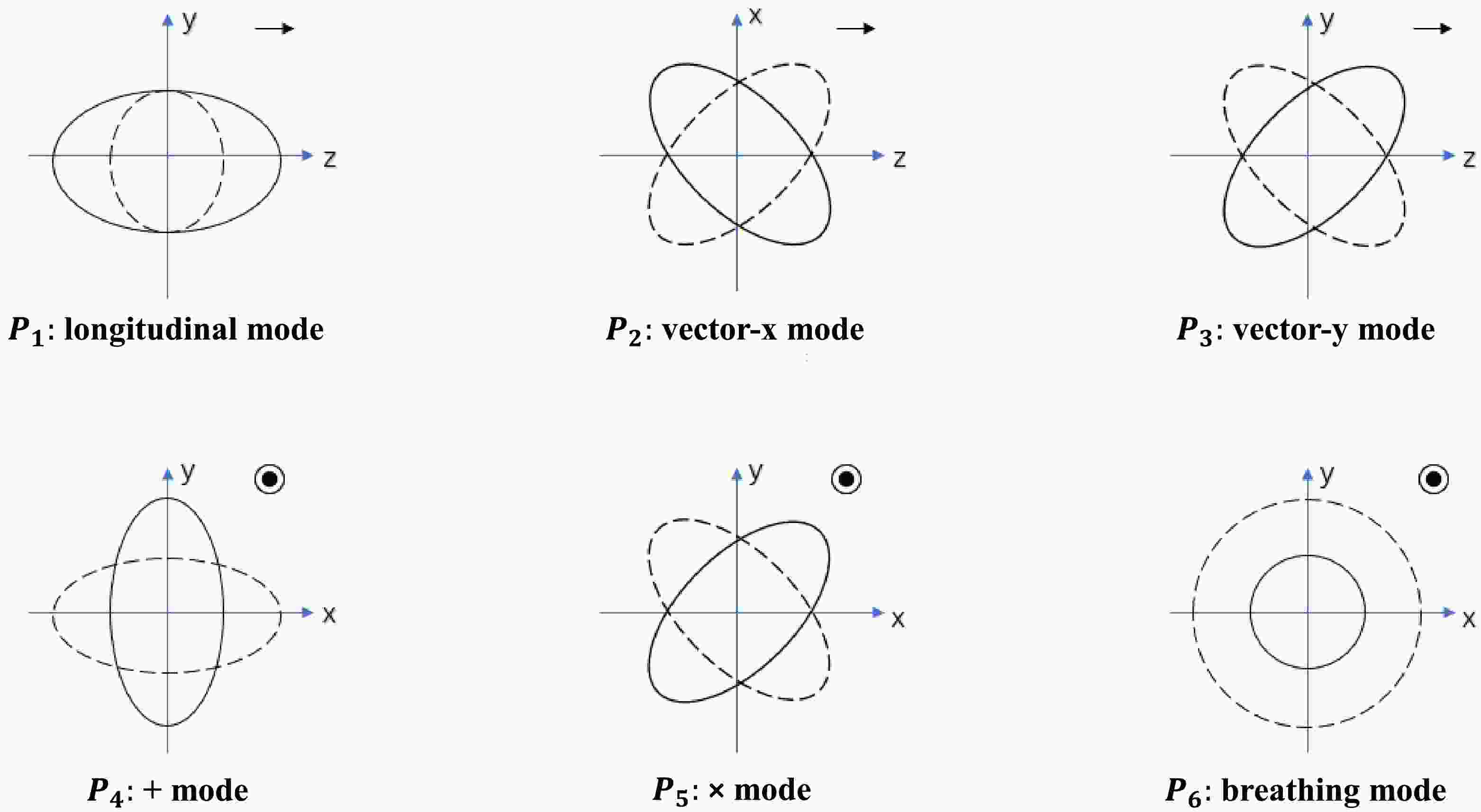
$ P_{1},..., P_{6} $ define six independent polarization modes of gravitational waves, and the corresponding relative motion of test particles in these modes is illustrated in Fig. 1. Figure 1 also labels the names corresponding to these six modes. The six modes are related to gauge-invariant perturbations as follows: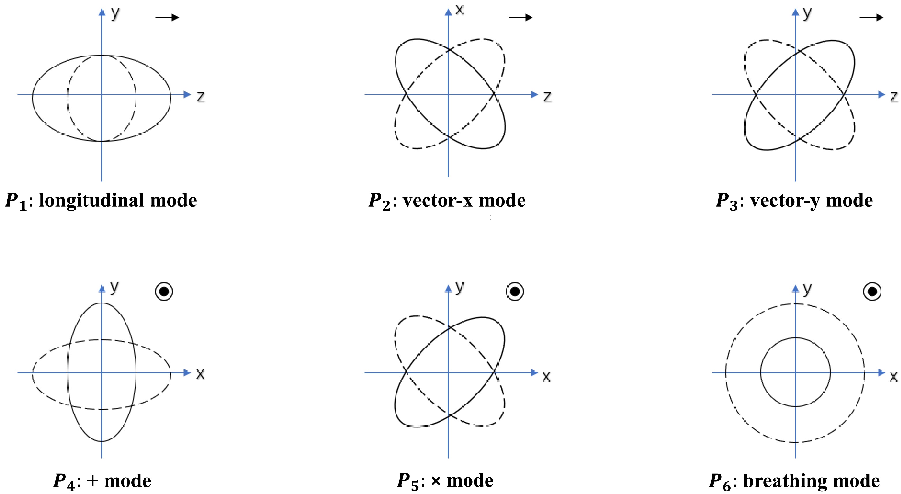
Figure 1. (color online) Six polarization modes of gravitational waves [28]. Here, the gravitational wave propagates in the
$ +z $ direction. We have labeled the names of the six polarization modes in the figure. Based on the relationship between different polarization modes and gauge-invariant perturbations, the$ + $ and × modes are referred to as tensor modes, the vector-x and vector-y modes are referred to as vector modes, and the breathing and longitudinal modes are referred to as scalar modes.$ \begin{aligned}[b] P_{1}=&\partial_{3}\partial_{3}\phi-\frac{1}{2}\partial_{0}\partial_{0}\Theta, \quad\quad P_{2}=\frac{1}{2}\partial_{0}\partial_{3}\Xi_{1},\\ P_{3}=&\frac{1}{2}\partial_{0}\partial_{3}\Xi_{2}, \qquad\quad\quad\quad P_{4}=-\frac{1}{2}\partial_{0}\partial_{0}h^{TT}_{11}, \\ P_{5}=&-\frac{1}{2}\partial_{0}\partial_{0}h^{TT}_{12}, \quad\qquad\;\;\; P_{6}=-\frac{1}{2}\partial_{0}\partial_{0}\Theta. \end{aligned} $
(29) In the presence of hypermomentum, we adopt the convective ansatz for test particles as in Refs. [58, 29]. Under this ansatz, the equation of relative motion for the test particles is given by
$ \begin{aligned}[b] & \frac{{\rm d}^2 \eta^{i}}{{\rm d}t^2} = -A^{i}_{\; j}\eta^{j} := -\widehat{R}^{i}_{\; 0j0}\eta^{j}-\partial_{j}N^{i}_{\; 00}\eta^{j}. \end{aligned} $
(30) Here,
$ \begin{aligned}[b] & N^{\lambda}_{\; \mu\nu}:= \Gamma^{\lambda}_{\; \mu\nu}-\widehat{\Gamma}^{\lambda}_{\; \mu\nu}. \end{aligned} $
(31) In this case,
$ A_{ij} $ is not symmetric in the indices$ (i, j) $ , which leads to two new polarization modes of gravitational waves$ P_{7}, P_{8} $ :$ \begin{aligned}[b] A_{ij}=\begin{pmatrix} P_{4}+P_{6} & P_{5} & P_{2}+P_{7}\\ P_{5} & -P_{4}+P_{6} & P_{3}+P_{8}\\ P_{2} & P_{3} & P_{1} \end{pmatrix}. \end{aligned} $
(32) It is thus evident that, when particles carry hypermomentum, the relative motion of test particles in the geodesic deviation equation is modified, increasing the number of possible independent motion modes from six to eight. The two new polarization modes,
$ P_{7} $ and$ P_{8} $ , are referred to as shear modes [29]. The relative motion of test particles in these two modes is illustrated in Fig. 2. The relationship between the polarization modes and gauge-invariant perturbations in this case is given by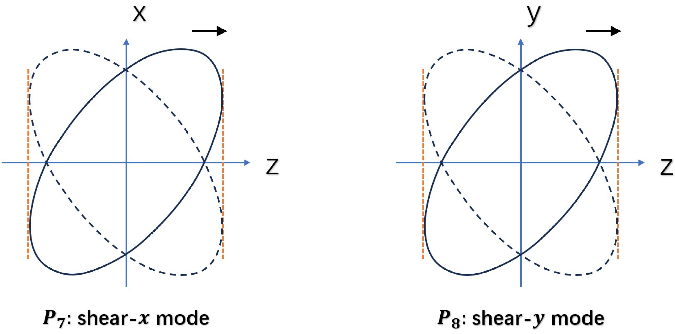
Figure 2. (color online) The two new shear modes [29].
$ \begin{aligned}[b] &P_{1}=\partial_{0}\partial_{0}\Theta -\partial_{3}\partial_{3}\Pi-\partial_{0}\partial_{3}\partial_{3}\bar{\Pi} -\frac{1}{2}\partial_{0}\partial_{0}L,\; P_{6}=-\frac{1}{2}\partial_{0}\partial_{0}\Theta, \\ &P_{2}=\frac{1}{2}\partial_{0}\partial_{3}\Xi_{1},\quad P_{3}=\frac{1}{2}\partial_{0}\partial_{3}\Xi_{2}, \\ &P_{4}=-\frac{1}{2}\partial_{0}\partial_{0}h^{TT}_{11}, \quad P_{5}=-\frac{1}{2}\partial_{0}\partial_{0}h^{TT}_{12}, \\ &P_{7}=\partial_{3}\Omega_{1} -\partial_{0}\partial_{3}K_{1},\quad P_{8}=\partial_{3}\Omega_{2} -\partial_{0}\partial_{3}K_{2}. \end{aligned} $
(33) Equation (30) does not describe the relative motion of a generic test particle carrying hypermomentum. Rather, our analysis is restricted to a specific class of test particles satisfying the convective ansatz. After introducing a quantity called the canonical energy–momentum tensor
$ \Sigma^{\mu}_{\; \lambda} $ ,$ \begin{aligned}[b] \Sigma^{\mu}_{\; \lambda} =T^{\mu}_{\; \lambda}+\frac{1}{2\sqrt{-g}}\nabla_{\nu}\left(\sqrt{-g}{\cal{H}}_{\lambda}^{\; \mu\nu}\right), \end{aligned} $
(34) the convective ansatz of Ref. [58] can be expressed as the following assumption:
$ \begin{aligned}[b] T^{\mu\nu}\left(t,{\bf{x}}\right) =& \frac{1}{\sqrt{-g}}\frac{mu^{\mu}u^{\nu}}{u^{0}}\delta^{3}\left({\bf{x}}-{\bf{X}}\left(t\right)\right), \end{aligned} $
(35) $ \begin{aligned}[b] {\cal{H}}_{\lambda}^{\; \mu\nu}\left(t,{\bf{x}}\right) =& \frac{1}{\sqrt{-g}}\frac{H_{\lambda}^{\; \mu}u^{\nu}}{u^{0}}\delta^{3}\left({\bf{x}}-{\bf{X}}\left(t\right)\right), \end{aligned} $
(36) $ \begin{aligned}[b] \Sigma^{\mu}_{\; \nu}\left(t,{\bf{x}}\right) =& \frac{1}{\sqrt{-g}}\frac{P_{\nu}u^{\mu}}{u^{0}}\delta^{3}\left({\bf{x}}-{\bf{X}}\left(t\right)\right). \end{aligned} $
(37) This ansatz corresponds to adopting the monopole approximation for
$ T^{\mu\nu}, {\cal{H}}_{\lambda}^{\; \mu\nu} $ , and$ \Sigma^{\mu}_{\; \nu} $ in deriving the test particle equations of motion from the conservation laws that follow from the diffeomorphism invariance of the matter action via a multipole expansion. However, for a general test particle carrying hypermomentum, there is no justification for assuming that the above approximation holds in all cases. Under the convective ansatz, the equation of motion for the test particles exhibits properties independent of the mass of the particle and the magnitude of its hypermomentum. However, different types of hypermomentum-carrying particles could lead to distinct equations of motion, potentially resulting in qualitatively different gravitational wave polarization structures.An additional intriguing question is whether a Lagrangian for the test particles can be found that satisfies the convective ansatz. To address this, we cite the results from a recent study [59], which investigates the Lagrangian mechanics of a class of test particles with the internal structure in the context of metric-affine geometry. In this framework, the internal structure of the test particles is described by a material frame (a tetrad) field
$ e^{a}_{\mu} $ , where$ (a=0,1,2,3) $ . In the presence of a gravitational field, the Lagrangian considered in Ref. [59] takes the following form:$ S_{m}=\int L \left[ v^{\mu}, e^{a}_{\mu}, \dot{e^{a}_{\mu}}, g_{\mu\nu} \right] {\rm d}\lambda. $
(38) Here, λ is used to parameterize the worldline of the test particle, with
$v^{\mu} := {\rm d}x^{\mu}/{\rm d}\lambda$ and$ \dot{e^{a}_{\mu}} := v^{\nu}\nabla_{\nu}e^{a}_{\mu} $ . Clearly, the coupling between the connection and the matter field occurs solely through$ \dot{e^{a}_{\mu}} $ . By varying the above Lagrangian, the authors of Ref. [59] obtained a set of equations describing the motion of the test particles, which are consistent with the results derived from the conservation laws via the multipole expansion method. We find that the following special case of the above Lagrangian,$ \begin{aligned}[b] S_{m}= -m\int\sqrt{-g_{\mu\nu}v^{\mu}v^{\nu}} {\rm d}\lambda + \int L_1 \left[ v^{\mu}, e^{a}_{\mu}, \dot{e^{a}_{\mu}}, \right] {\rm d}\lambda, \end{aligned} $
(39) with
$ \dot{e^{a}_{\mu}} $ in$ L_1 $ coupling only to$ v^{\mu} $ , yields field equations that coincide with those considered in our analysis. In particular, Eq. (30) can be directly derived from the equation obtained by varying with respect to$ e^{a}_{\mu} $ . Interestingly, if the matter action satisfies Eq. (39), the equation of relative motion for test particles remains Eq. (30), even in the presence of torsion.Finally, it should be emphasized that we have introduced a kinematical definition of gravitational wave polarization modes based on the independent relative motion modes of test particles, which provides the maximal set of possible independent polarization modes in the most general case. However, for a given specific gravitational theory, not all of these modes are necessarily excited. To determine the modes that are allowed, one must first solve the linearized perturbation equations to identify the structure of propagating degrees of freedom in that theory. Subsequently, by analyzing how each propagating degree of freedom affects the relative motion of test particles, one can determine the polarization modes allowed by the theory. Since the relative motion of test particles is observable, these polarization modes correspond to measurable physical quantities rather than gauge artifacts. It should be further clarified that the gravitational-wave polarization modes defined here and the propagating (or intrinsic dynamical) degrees of freedom of gravitational waves are conceptually distinct. The propagating degrees of freedom are determined by the number of independent solutions to the linearized perturbation equations and thus represent an intrinsic property of the gravitational theory itself, independent of the specific characteristics of test particles (e.g., whether they carry hypermomentum). In contrast, gravitational-wave polarization modes are defined via the response of test particles and therefore depend on the properties of the probing matter, including whether the test particles carry hypermomentum.
-
To study the polarization modes of gravitational waves, we need to solve the linearized field equations of the theory. Before doing so, we first introduce the basic concepts of gauge-invariant perturbations and gravitational wave polarization modes in this section.
The gauge-invariant perturbation method can significantly simplify the linearized field equations. This approach allows us to reformulate the variables in the linearized field equations in terms of a set of gauge-invariant tensors, vectors, and scalars (in the sense of spatial rotations). Furthermore, by decoupling the linearized field equations, we obtain a series of tensor, vector, and scalar equations, each of which depends solely on the corresponding gauge-invariant tensor, vector, or scalar. This method has been elaborated in detail in Refs. [29, 39, 45, 53−55]; here, we only summarize the necessary results.
It is well known that perturbations can be uniquely decomposed into scalar, vector, and tensor components, following the standard scalar–vector–tensor decomposition [29, 53−57]
$ \begin{aligned}[b] h_{00}=&h_{00}, \qquad h_{0i}=\partial_{i}\gamma+\beta_{i},\\ h_{ij}=&h^{TT}_{ij}+\partial_{i}\epsilon_{j}+\partial_{j}\epsilon_{i} +\frac{1}{3}\delta_{ij}H+\left(\partial_{i}\partial_{j}-\frac{1}{3}\delta_{ij}\Delta\right)\zeta, \end{aligned} $
$ \begin{aligned}[b] \Sigma^{0}_{\; 00}=&\Sigma^{0}_{\; 00}, \\ \Sigma^{i}_{\; 00}=&\partial_{i}F+G_{i}, \\ \Sigma^{0}_{\; 0i}=&\partial_{i}M+N_{i}, \\ \Sigma^{0}_{\; ij}=&S_{ij}+\partial_{i}C_{j}+\partial_{j}C_{i}+\partial_{i}\partial_{j}B+\delta_{ij}A, \\ \Sigma^{i}_{\; 0j}=&U_{ij}+V_{ij}+\partial_{i}\bar{C}_{j}+\partial_{j}\bar{D}_{i}+\partial_{i}\partial_{j}\bar{B}+\delta_{ij}\bar{A}, \\ \Sigma^{i}_{\; jk}=&B^{i}_{\; jk}+\partial_{i}C_{jk}+\partial_{j}D_{ik}+\partial_{k}D_{ij}+\partial_{j}E_{ik}+\partial_{k}E_{ij} \\ &+\partial_{i}\partial_{j}f_{k}+\partial_{i}\partial_{k}f_{j}+\partial_{j}\partial_{k}g_{i}+\delta_{jk}h_{i}+\delta_{ij}q_{k}+\delta_{ik}q_{j}\\ &+\partial_{i}\partial_{j}\partial_{k}l+\delta_{jk}\partial_{i}m+\delta_{ij}\partial_{k}n+\delta_{ik}\partial_{j}n, \end{aligned} $
(18) where some constraints have been imposed:
$ \begin{aligned}[b] \partial_{i}\beta^{i}=&\partial_{i}\epsilon^{i}=\partial_{i}G^i=\partial_{i}N^i=\partial_{i}C^i=\partial_{i}{\bar{C}}^i=\partial_{i}{\bar{D}}^i\\ =&\partial_{i}f^i=\partial_{i}g^i=\partial_{i}h^i=\partial_{i}q^i=0, \\ h^{TTi}_{\; \; \; \; i}=&S^{i}_{\; i}=U^{i}_{\; i}=V^{i}_{\; i}=C^{i}_{\; i}=D^{i}_{\; i}=E^{i}_{\; i}=0, \\ \partial_{i}h^{TTi}_{\; \; \; \; j}=&\partial_{i}S^{i}_{\; j}=\partial_{i}U^{i}_{\; j}=\partial_{i}V^{i}_{\; j}=\partial_{i}C^{i}_{\; j}=\partial_{i}D^{i}_{\; j}=\partial_{i}E^{i}_{\; j}=0, \\ h^{TT}_{ij}=&h^{TT}_{ji},\; S_{ij}=S_{ji},\; U_{ij}=U_{ji},\; C_{ij}=C_{ji}, \\ D_{ij}=&D_{ji},\; V_{ij}=-V_{ji},\; E_{ij}=-E_{ji}, \\ B^{i}_{\; jk}=& B^{i}_{\; kj},\; B^{i}_{\; ik}=B^{i}_{\; jk}\delta^{jk}=0,\; \partial_{i}B^{i}_{\; jk}=\partial^{j}B^{i}_{\; jk}=0. \end{aligned} $
(19) Here, each variable on the right-hand side of the equations corresponds to the scalar, vector, or tensor component obtained from this decomposition. These components are determined by solving the corresponding Poisson-type equations. Spatial indices are raised and lowered by
$ \delta_{ij} $ , and thus, there is no need to distinguish between upper and lower spatial indices. Considering that, under a gauge transformation (infinitesimal coordinate transformation),$ x^\mu \rightarrow x^\mu+\xi^{\mu}(x) $ , where$ \xi^{\mu} $ denotes an arbitrary vector function, we have$ \begin{aligned}[b] h_{\mu\nu} \rightarrow h_{\mu\nu}-\partial_{\mu}\xi_{\nu}-\partial_{\nu}\xi_{\mu}, \quad \Sigma^{\lambda}_{\; \mu\nu} \rightarrow \Sigma^{\lambda}_{\; \mu\nu}+\partial_{\mu}\partial_{\nu}\xi^{\lambda}. \end{aligned} $
(20) Then, we can construct the following gauge-invariant perturbations [29]:
● Transverse traceless third-order spatial tensor:
$ \begin{aligned}[b] B^{i}_{\; jk}. \end{aligned} $
(21) ● Transverse traceless second-order spatial tensors:
$ \begin{aligned}[b] h^{TT}_{ij},\; S_{ij},\; U_{ij},\; V_{ij},\; C_{ij},\; D_{ij},\; E_{ij}. \end{aligned} $
(22) ● Transverse spatial vectors:
$ \begin{aligned}[b] &N_{i},\; C_{i},\; \bar{C}_{i},\; f_{i},\; h_{i},\; q_{i}, \\ &\Xi_{i}:= \beta_{i}-\partial_{0}\epsilon_{i}, \\ &\Omega_{i}:= G_{i}-\partial_{0}\bar{D}_{i},\; \bar{\Omega}_{i}:= \bar{D}_{i}-\partial_{0}g_{i},\; K_{i}:=\beta_{i}+\bar{D}_{i}. \end{aligned} $
(23) ● Spatial scalars:
$ \begin{aligned}[b] &A,\; \bar{A},\; m,\; n, \\ &\Theta:= \frac{1}{3}\left(H-\Delta\zeta\right),\; \phi:= -\frac{1}{2}h_{00}+\partial_{0}\gamma-\frac{1}{2}\partial_{0}^{2}\zeta, \\ &\Psi:= \Sigma^{0}_{\; 00}-\partial_{0}M,\; \bar{\Psi}:= M-\partial_{0}B, \\ &\Pi:= F-\partial_{0}\bar{B},\; \bar{\Pi}:= \bar{B}-\partial_{0}{l}, \\ &K := -h_{00}+2M,\; L := H+2\Delta l. \end{aligned} $
(24) This concludes all the necessary background on gauge-invariant perturbations. Now, we turn to the fundamental concepts of gravitational wave polarization modes. The polarization modes of gravitational waves are defined through the independent relative motion modes of test particles. For the case without hypermomentum, the equation of relative motion between two test particles is the well-known one:
$ \frac{{\rm d}^2 \eta^{i}}{{\rm d}t^2} = -\widehat{R}^{i}_{\; 0j0}\eta^{j}. $
(25) Here,
$ \eta^{i} $ denotes the relative displacement between two test particles. It is always possible, without loss of generality, to consider the case where gravitational waves propagate along the$ +z $ direction. Therefore, all gravitational waves discussed in this paper are set to propagate in the$ +z $ direction. Under this assumption, the monochromatic plane wave leads to$ \widehat{R}_{i0j0}=A_{0} E_{ij} {\rm e}^{{\rm i}kx}. $
(26) Here,
$ k^{\mu} $ is the four-wavevector,$ A_{0} $ represents the wave intensity, and$ E_{ij} $ is a$ 3 \times 3 $ matrix encapsulating all polarization information of this plane wave, which satisfies$ E_{ij}E^{ij}=1. $
(27) Due to the symmetry of the
$ (i, j) $ indices in$ \widehat{R}_{i0j0} $ , there can be at most six independent gravitational wave polarization modes in this case:$ \begin{aligned}[b] \widehat{R}_{i0j0}=\begin{pmatrix} P_{4}+P_{6} & P_{5} & P_{2}\\ P_{5} & -P_{4}+P_{6} & P_{3}\\ P_{2} & P_{3} & P_{1} \end{pmatrix}. \end{aligned} $
(28) Here,
$ P_{1},..., P_{6} $ define six independent polarization modes of gravitational waves, and the corresponding relative motion of test particles in these modes is illustrated in Fig. 1. Figure 1 also labels the names corresponding to these six modes. The six modes are related to gauge-invariant perturbations as follows:
Figure 1. (color online) Six polarization modes of gravitational waves [28]. Here, the gravitational wave propagates in the
$ +z $ direction. We have labeled the names of the six polarization modes in the figure. Based on the relationship between different polarization modes and gauge-invariant perturbations, the$ + $ and × modes are referred to as tensor modes, the vector-x and vector-y modes are referred to as vector modes, and the breathing and longitudinal modes are referred to as scalar modes.$ \begin{aligned}[b] P_{1}=&\partial_{3}\partial_{3}\phi-\frac{1}{2}\partial_{0}\partial_{0}\Theta, \quad\quad P_{2}=\frac{1}{2}\partial_{0}\partial_{3}\Xi_{1},\\ P_{3}=&\frac{1}{2}\partial_{0}\partial_{3}\Xi_{2}, \qquad\quad\quad\quad P_{4}=-\frac{1}{2}\partial_{0}\partial_{0}h^{TT}_{11}, \\ P_{5}=&-\frac{1}{2}\partial_{0}\partial_{0}h^{TT}_{12}, \quad\qquad\;\;\; P_{6}=-\frac{1}{2}\partial_{0}\partial_{0}\Theta. \end{aligned} $
(29) In the presence of hypermomentum, we adopt the convective ansatz for test particles as in Refs. [58, 29]. Under this ansatz, the equation of relative motion for the test particles is given by
$ \begin{aligned}[b] & \frac{{\rm d}^2 \eta^{i}}{{\rm d}t^2} = -A^{i}_{\; j}\eta^{j} := -\widehat{R}^{i}_{\; 0j0}\eta^{j}-\partial_{j}N^{i}_{\; 00}\eta^{j}. \end{aligned} $
(30) Here,
$ \begin{aligned}[b] & N^{\lambda}_{\; \mu\nu}:= \Gamma^{\lambda}_{\; \mu\nu}-\widehat{\Gamma}^{\lambda}_{\; \mu\nu}. \end{aligned} $
(31) In this case,
$ A_{ij} $ is not symmetric in the indices$ (i, j) $ , which leads to two new polarization modes of gravitational waves$ P_{7}, P_{8} $ :$ \begin{aligned}[b] A_{ij}=\begin{pmatrix} P_{4}+P_{6} & P_{5} & P_{2}+P_{7}\\ P_{5} & -P_{4}+P_{6} & P_{3}+P_{8}\\ P_{2} & P_{3} & P_{1} \end{pmatrix}. \end{aligned} $
(32) It is thus evident that, when particles carry hypermomentum, the relative motion of test particles in the geodesic deviation equation is modified, increasing the number of possible independent motion modes from six to eight. The two new polarization modes,
$ P_{7} $ and$ P_{8} $ , are referred to as shear modes [29]. The relative motion of test particles in these two modes is illustrated in Fig. 2. The relationship between the polarization modes and gauge-invariant perturbations in this case is given by
Figure 2. (color online) The two new shear modes [29].
$ \begin{aligned}[b] &P_{1}=\partial_{0}\partial_{0}\Theta -\partial_{3}\partial_{3}\Pi-\partial_{0}\partial_{3}\partial_{3}\bar{\Pi} -\frac{1}{2}\partial_{0}\partial_{0}L,\; P_{6}=-\frac{1}{2}\partial_{0}\partial_{0}\Theta, \\ &P_{2}=\frac{1}{2}\partial_{0}\partial_{3}\Xi_{1},\quad P_{3}=\frac{1}{2}\partial_{0}\partial_{3}\Xi_{2}, \\ &P_{4}=-\frac{1}{2}\partial_{0}\partial_{0}h^{TT}_{11}, \quad P_{5}=-\frac{1}{2}\partial_{0}\partial_{0}h^{TT}_{12}, \\ &P_{7}=\partial_{3}\Omega_{1} -\partial_{0}\partial_{3}K_{1},\quad P_{8}=\partial_{3}\Omega_{2} -\partial_{0}\partial_{3}K_{2}. \end{aligned} $
(33) Equation (30) does not describe the relative motion of a generic test particle carrying hypermomentum. Rather, our analysis is restricted to a specific class of test particles satisfying the convective ansatz. After introducing a quantity called the canonical energy–momentum tensor
$ \Sigma^{\mu}_{\; \lambda} $ ,$ \begin{aligned}[b] \Sigma^{\mu}_{\; \lambda} =T^{\mu}_{\; \lambda}+\frac{1}{2\sqrt{-g}}\nabla_{\nu}\left(\sqrt{-g}{\cal{H}}_{\lambda}^{\; \mu\nu}\right), \end{aligned} $
(34) the convective ansatz of Ref. [58] can be expressed as the following assumption:
$ \begin{aligned}[b] T^{\mu\nu}\left(t,{\bf{x}}\right) =& \frac{1}{\sqrt{-g}}\frac{mu^{\mu}u^{\nu}}{u^{0}}\delta^{3}\left({\bf{x}}-{\bf{X}}\left(t\right)\right), \end{aligned} $
(35) $ \begin{aligned}[b] {\cal{H}}_{\lambda}^{\; \mu\nu}\left(t,{\bf{x}}\right) =& \frac{1}{\sqrt{-g}}\frac{H_{\lambda}^{\; \mu}u^{\nu}}{u^{0}}\delta^{3}\left({\bf{x}}-{\bf{X}}\left(t\right)\right), \end{aligned} $
(36) $ \begin{aligned}[b] \Sigma^{\mu}_{\; \nu}\left(t,{\bf{x}}\right) =& \frac{1}{\sqrt{-g}}\frac{P_{\nu}u^{\mu}}{u^{0}}\delta^{3}\left({\bf{x}}-{\bf{X}}\left(t\right)\right). \end{aligned} $
(37) This ansatz corresponds to adopting the monopole approximation for
$ T^{\mu\nu}, {\cal{H}}_{\lambda}^{\; \mu\nu} $ , and$ \Sigma^{\mu}_{\; \nu} $ in deriving the test particle equations of motion from the conservation laws that follow from the diffeomorphism invariance of the matter action via a multipole expansion. However, for a general test particle carrying hypermomentum, there is no justification for assuming that the above approximation holds in all cases. Under the convective ansatz, the equation of motion for the test particles exhibits properties independent of the mass of the particle and the magnitude of its hypermomentum. However, different types of hypermomentum-carrying particles could lead to distinct equations of motion, potentially resulting in qualitatively different gravitational wave polarization structures.An additional intriguing question is whether a Lagrangian for the test particles can be found that satisfies the convective ansatz. To address this, we cite the results from a recent study [59], which investigates the Lagrangian mechanics of a class of test particles with the internal structure in the context of metric-affine geometry. In this framework, the internal structure of the test particles is described by a material frame (a tetrad) field
$ e^{a}_{\mu} $ , where$ (a=0,1,2,3) $ . In the presence of a gravitational field, the Lagrangian considered in Ref. [59] takes the following form:$ S_{m}=\int L \left[ v^{\mu}, e^{a}_{\mu}, \dot{e^{a}_{\mu}}, g_{\mu\nu} \right] {\rm d}\lambda. $
(38) Here, λ is used to parameterize the worldline of the test particle, with
$v^{\mu} := {\rm d}x^{\mu}/{\rm d}\lambda$ and$ \dot{e^{a}_{\mu}} := v^{\nu}\nabla_{\nu}e^{a}_{\mu} $ . Clearly, the coupling between the connection and the matter field occurs solely through$ \dot{e^{a}_{\mu}} $ . By varying the above Lagrangian, the authors of Ref. [59] obtained a set of equations describing the motion of the test particles, which are consistent with the results derived from the conservation laws via the multipole expansion method. We find that the following special case of the above Lagrangian,$ \begin{aligned}[b] S_{m}= -m\int\sqrt{-g_{\mu\nu}v^{\mu}v^{\nu}} {\rm d}\lambda + \int L_1 \left[ v^{\mu}, e^{a}_{\mu}, \dot{e^{a}_{\mu}}, \right] {\rm d}\lambda, \end{aligned} $
(39) with
$ \dot{e^{a}_{\mu}} $ in$ L_1 $ coupling only to$ v^{\mu} $ , yields field equations that coincide with those considered in our analysis. In particular, Eq. (30) can be directly derived from the equation obtained by varying with respect to$ e^{a}_{\mu} $ . Interestingly, if the matter action satisfies Eq. (39), the equation of relative motion for test particles remains Eq. (30), even in the presence of torsion.Finally, it should be emphasized that we have introduced a kinematical definition of gravitational wave polarization modes based on the independent relative motion modes of test particles, which provides the maximal set of possible independent polarization modes in the most general case. However, for a given specific gravitational theory, not all of these modes are necessarily excited. To determine the modes that are allowed, one must first solve the linearized perturbation equations to identify the structure of propagating degrees of freedom in that theory. Subsequently, by analyzing how each propagating degree of freedom affects the relative motion of test particles, one can determine the polarization modes allowed by the theory. Since the relative motion of test particles is observable, these polarization modes correspond to measurable physical quantities rather than gauge artifacts. It should be further clarified that the gravitational-wave polarization modes defined here and the propagating (or intrinsic dynamical) degrees of freedom of gravitational waves are conceptually distinct. The propagating degrees of freedom are determined by the number of independent solutions to the linearized perturbation equations and thus represent an intrinsic property of the gravitational theory itself, independent of the specific characteristics of test particles (e.g., whether they carry hypermomentum). In contrast, gravitational-wave polarization modes are defined via the response of test particles and therefore depend on the properties of the probing matter, including whether the test particles carry hypermomentum.
-
In this section, we analyze the gravitational wave polarization modes in general symmetric teleparallel gravity, which can yield second-order field equations. We need to solve Eqs. (11)−(13), where the explicit expressions for
$ {\cal{F}}_{\mu\nu} $ and$ {\cal{G}}_{\lambda}^{\; \mu\nu} $ are obtained from the variation of action (14).We first examine Eq. (13), which requires the curvature to be zero. When rewriting this equation in terms of the gauge-invariant perturbations from the previous section, we obtain
$ \begin{aligned}[b] B^{i}_{ jk}&=0,\; S_{ij}=U_{ij}=V_{ij}=C_{ij}=D_{ij}=E_{ij}=0, \\ N_{i}&=C_{i}=\bar{C}_{i}=\Omega_{i}=\bar{\Omega}_{i}=f_{i}=h_{i}=q_{i}=0, \\ \Psi&=\bar{\Psi}=A=\bar{A}=\Pi=\bar{\Pi}=m=n=0. \end{aligned} $
(40) It can be seen that, for gauge-invariant tensor perturbations, only
$ h^{TT}_{ij} $ may propagate. Similarly, for vector perturbations, only$ \Xi_{i} $ and$ K_{i} $ may propagate, and for scalar perturbations, only Θ, Φ, K, and L may propagate. Equation (40) requires that all gauge-invariant perturbations composed solely of connection perturbations vanish, which is consistent with the fact that, in symmetric teleparallel gravity, one can always choose the coincident gauge:$ \Gamma^{\lambda}_{\; \mu\nu}=0 $ [6].Now, we consider the remaining Eqs. (11) and (12) by separately analyzing the tensor, vector, and scalar equations.
-
In this section, we analyze the gravitational wave polarization modes in general symmetric teleparallel gravity, which can yield second-order field equations. We need to solve Eqs. (11)−(13), where the explicit expressions for
$ {\cal{F}}_{\mu\nu} $ and$ {\cal{G}}_{\lambda}^{\; \mu\nu} $ are obtained from the variation of action (14).We first examine Eq. (13), which requires the curvature to be zero. When rewriting this equation in terms of the gauge-invariant perturbations from the previous section, we obtain
$ \begin{aligned}[b] B^{i}_{ jk}&=0,\; S_{ij}=U_{ij}=V_{ij}=C_{ij}=D_{ij}=E_{ij}=0, \\ N_{i}&=C_{i}=\bar{C}_{i}=\Omega_{i}=\bar{\Omega}_{i}=f_{i}=h_{i}=q_{i}=0, \\ \Psi&=\bar{\Psi}=A=\bar{A}=\Pi=\bar{\Pi}=m=n=0. \end{aligned} $
(40) It can be seen that, for gauge-invariant tensor perturbations, only
$ h^{TT}_{ij} $ may propagate. Similarly, for vector perturbations, only$ \Xi_{i} $ and$ K_{i} $ may propagate, and for scalar perturbations, only Θ, Φ, K, and L may propagate. Equation (40) requires that all gauge-invariant perturbations composed solely of connection perturbations vanish, which is consistent with the fact that, in symmetric teleparallel gravity, one can always choose the coincident gauge:$ \Gamma^{\lambda}_{\; \mu\nu}=0 $ [6].Now, we consider the remaining Eqs. (11) and (12) by separately analyzing the tensor, vector, and scalar equations.
-
The equation for the tensor perturbation is given by
$ \begin{aligned}[b] & A_{(2)}\Box h^{TT}_{ij}=0. \end{aligned} $
(41) Combining Eqs. (29) and (33), this implies that symmetric teleparallel gravity necessarily requires
$ A_{(2)} \neq 0 $ , and there must exist$ + $ and × modes propagating at the speed of light, regardless of whether the test particles carry hypermomentum charge. -
The equation for the tensor perturbation is given by
$ \begin{aligned}[b] & A_{(2)}\Box h^{TT}_{ij}=0. \end{aligned} $
(41) Combining Eqs. (29) and (33), this implies that symmetric teleparallel gravity necessarily requires
$ A_{(2)} \neq 0 $ , and there must exist$ + $ and × modes propagating at the speed of light, regardless of whether the test particles carry hypermomentum charge. -
There are three vector equations:
$ \begin{aligned}[b] 4A_{(2)}\Delta\Xi_{i} +\left(C_{(1)}+E_{(1)}\right) \left[\partial_{0}^{2}K_{i} +\Delta\left(\Xi_{i}-K_{i}\right)\right] =& 0, \end{aligned} $
(42) $ \begin{aligned}[b] 4A_{(2)}\partial_{0}^{2}\Xi_{i} +\left(C_{(1)}+E_{(1)}\right) \left[ \partial_{0}^{2}K_{i} +\Delta\left(\Xi_{i}-K_{i}\right) \right] =& 0, \end{aligned} $
(43) $ \begin{aligned}[b] \left(C_{(1)}+E_{(1)}\right)\Box \left[\partial_{0}^{2}K_{i} +\Delta\left(\Xi_{i}-K_{i}\right)\right] =& 0. \end{aligned} $
(44) Since these equations are linear, they can be transformed into an algebraic system by rewriting them in momentum space form to facilitate solving [29, 46]. The results show that, when
$ 4A_{(2)}+C_{(1)}+E_{(1)}=0 $ ,$ \Xi_{i} $ propagates at the speed of light. According to Eqs. (29) and (33), this implies the existence of vector-x and vector-y modes that propagate at the speed of light. For any other parameters,$ \Xi_{i}=0 $ , and vector-x and vector-y modes do not exist. In particular, when the test particles do not carry hypermomentum charge, vector mode gravitational waves emerge solely within a specific parameter space, as dictated by Eq. (29).We find that, when
$ C_{(1)}+E_{(1)} \neq 0 $ , there exists a solution for the perturbation$ K_{i} $ and it propagates at the speed of light. However, when$ C_{(1)}+E_{(1)}=0 $ ,$ K_{i} $ is not constrained by any equation. This indicates that the variable$ K_{i} $ does not appear in the linear perturbation equations, implying that its dynamical information is entirely encoded at nonlinear order. In other words, the linear perturbation theory breaks down in this case, and its dynamics can only be determined by including higher-order terms in the perturbative expansion, where nonlinear interactions become essential. This feature further suggests that, when$ C_{(1)}+E_{(1)}=0 $ , the quadratic action does not provide a standard kinetic structure for$ K_{i} $ , and its behavior may be governed predominantly by nonlinear terms. Consequently, the standard perturbative expansion around the Minkowski background (5) may require a more careful treatment beyond linear order. Such features have been observed in various symmetric teleparallel gravity models [60−62]. -
There are three vector equations:
$ \begin{aligned}[b] 4A_{(2)}\Delta\Xi_{i} +\left(C_{(1)}+E_{(1)}\right) \left[\partial_{0}^{2}K_{i} +\Delta\left(\Xi_{i}-K_{i}\right)\right] =& 0, \end{aligned} $
(42) $ \begin{aligned}[b] 4A_{(2)}\partial_{0}^{2}\Xi_{i} +\left(C_{(1)}+E_{(1)}\right) \left[ \partial_{0}^{2}K_{i} +\Delta\left(\Xi_{i}-K_{i}\right) \right] =& 0, \end{aligned} $
(43) $ \begin{aligned}[b] \left(C_{(1)}+E_{(1)}\right)\Box \left[\partial_{0}^{2}K_{i} +\Delta\left(\Xi_{i}-K_{i}\right)\right] =& 0. \end{aligned} $
(44) Since these equations are linear, they can be transformed into an algebraic system by rewriting them in momentum space form to facilitate solving [29, 46]. The results show that, when
$ 4A_{(2)}+C_{(1)}+E_{(1)}=0 $ ,$ \Xi_{i} $ propagates at the speed of light. According to Eqs. (29) and (33), this implies the existence of vector-x and vector-y modes that propagate at the speed of light. For any other parameters,$ \Xi_{i}=0 $ , and vector-x and vector-y modes do not exist. In particular, when the test particles do not carry hypermomentum charge, vector mode gravitational waves emerge solely within a specific parameter space, as dictated by Eq. (29).We find that, when
$ C_{(1)}+E_{(1)} \neq 0 $ , there exists a solution for the perturbation$ K_{i} $ and it propagates at the speed of light. However, when$ C_{(1)}+E_{(1)}=0 $ ,$ K_{i} $ is not constrained by any equation. This indicates that the variable$ K_{i} $ does not appear in the linear perturbation equations, implying that its dynamical information is entirely encoded at nonlinear order. In other words, the linear perturbation theory breaks down in this case, and its dynamics can only be determined by including higher-order terms in the perturbative expansion, where nonlinear interactions become essential. This feature further suggests that, when$ C_{(1)}+E_{(1)}=0 $ , the quadratic action does not provide a standard kinetic structure for$ K_{i} $ , and its behavior may be governed predominantly by nonlinear terms. Consequently, the standard perturbative expansion around the Minkowski background (5) may require a more careful treatment beyond linear order. Such features have been observed in various symmetric teleparallel gravity models [60−62]. -
There are six scalar equations, which are relatively complex; therefore, we present the detailed forms of these equations in Appendix A. The properties of these scalar polarization modes depend on the parameter space, and their general analysis is very complex and tedious. However, two universal conclusions can still be drawn. The first one is that there always exists the following plane wave solution propagating at the speed of light:
$ L+K=0, \phi=\Theta=0 $ . Therefore, according to Eq. (33), in the case where the test particles have hypermomentum, there always exists a longitudinal mode propagating at the speed of light. The second one is that, owing to the homogeneity of the field equations and their formal Lorentz symmetry, all possible scalar modes must propagate at the speed of light. -
There are six scalar equations, which are relatively complex; therefore, we present the detailed forms of these equations in Appendix A. The properties of these scalar polarization modes depend on the parameter space, and their general analysis is very complex and tedious. However, two universal conclusions can still be drawn. The first one is that there always exists the following plane wave solution propagating at the speed of light:
$ L+K=0, \phi=\Theta=0 $ . Therefore, according to Eq. (33), in the case where the test particles have hypermomentum, there always exists a longitudinal mode propagating at the speed of light. The second one is that, owing to the homogeneity of the field equations and their formal Lorentz symmetry, all possible scalar modes must propagate at the speed of light. -
In this section, we describe the gravitational wave polarization modes in two typical symmetric teleparallel gravity theories:
$ f(Q) $ gravity and quadratic non-metricity gravity. -
In this section, we describe the gravitational wave polarization modes in two typical symmetric teleparallel gravity theories:
$ f(Q) $ gravity and quadratic non-metricity gravity. -
The action of
$ f(Q) $ gravity is given by$ \begin{aligned}[b] & {S_{g}} =\int {\rm d}^{4}x \sqrt{-g} f(Q), \end{aligned} $
(45) where
$ \begin{aligned}[b] & Q := \frac{1}{4}Q_{\alpha\mu\nu}Q^{\alpha\mu\nu} -\frac{1}{2}Q_{\alpha\mu\nu}Q^{\mu\alpha\nu} -\frac{1}{4}Q_{\alpha\lambda}^{\; \; \lambda}Q^{\alpha\rho}_{\; \; \rho} +\frac{1}{2}Q_{\alpha\lambda}^{\; \; \lambda}Q^{\rho\; \alpha}_{\; \rho}. \end{aligned} $
(46) Here,
$ f(Q) $ is an analytic function dependent on Q, and it can be expanded as$ \begin{aligned}[b] & f(Q)=\alpha Q+\beta Q^{2}+..., \end{aligned} $
(47) where α and β are theoretical parameters. By using the correspondence provided in Appendix F of Ref. [29], which relates the parameters in action (14) to combinations of the curvature tensor
$ R^{\mu}_{\; \nu\lambda\rho} $ and non-metricity$ Q_{\lambda\mu\nu} $ , one can directly observe that the parameters corresponding to the$ f(Q) $ theory are$ \begin{aligned}[b] & A_{(1)}=-\alpha,\; B_{(1)}=\frac{1}{2}\alpha,\; D_{(1)}=-\frac{1}{2}\alpha,\; A_{(2)}=-\frac{1}{4}\alpha, \end{aligned} $
(48) with all other parameters being zero.
By solving the linear perturbation equations, we find that this requires
$ \begin{aligned}[b] & \Xi_{i}=\Theta=\phi=0. \end{aligned} $
(49) Therefore, in the case where test particles do not have hypermomentum,
$ f(Q) $ theory only has tensor modes ($ + $ and × modes) propagating at the speed of light, without additional vector or scalar modes, which is consistent with the conclusion obtained in Ref. [44]. In the case with hypermomentum charge, at the level of linear perturbations, according to Eq. (33), we find that, in addition to the tensor modes propagating at the speed of light, the theory always has unconstrained shear modes and the unconstrained longitudinal mode. In$ f(Q) $ theory, the condition$ C_{(1)}+E_{(1)}=0 $ signals a potential strong-coupling problem. In fact, the presence of such a problem in$ f(Q) $ gravity has already been noted in Refs. [60, 61] -
The action of
$ f(Q) $ gravity is given by$ \begin{aligned}[b] & {S_{g}} =\int {\rm d}^{4}x \sqrt{-g} f(Q), \end{aligned} $
(45) where
$ \begin{aligned}[b] & Q := \frac{1}{4}Q_{\alpha\mu\nu}Q^{\alpha\mu\nu} -\frac{1}{2}Q_{\alpha\mu\nu}Q^{\mu\alpha\nu} -\frac{1}{4}Q_{\alpha\lambda}^{\; \; \lambda}Q^{\alpha\rho}_{\; \; \rho} +\frac{1}{2}Q_{\alpha\lambda}^{\; \; \lambda}Q^{\rho\; \alpha}_{\; \rho}. \end{aligned} $
(46) Here,
$ f(Q) $ is an analytic function dependent on Q, and it can be expanded as$ \begin{aligned}[b] & f(Q)=\alpha Q+\beta Q^{2}+..., \end{aligned} $
(47) where α and β are theoretical parameters. By using the correspondence provided in Appendix F of Ref. [29], which relates the parameters in action (14) to combinations of the curvature tensor
$ R^{\mu}_{\; \nu\lambda\rho} $ and non-metricity$ Q_{\lambda\mu\nu} $ , one can directly observe that the parameters corresponding to the$ f(Q) $ theory are$ \begin{aligned}[b] & A_{(1)}=-\alpha,\; B_{(1)}=\frac{1}{2}\alpha,\; D_{(1)}=-\frac{1}{2}\alpha,\; A_{(2)}=-\frac{1}{4}\alpha, \end{aligned} $
(48) with all other parameters being zero.
By solving the linear perturbation equations, we find that this requires
$ \begin{aligned}[b] & \Xi_{i}=\Theta=\phi=0. \end{aligned} $
(49) Therefore, in the case where test particles do not have hypermomentum,
$ f(Q) $ theory only has tensor modes ($ + $ and × modes) propagating at the speed of light, without additional vector or scalar modes, which is consistent with the conclusion obtained in Ref. [44]. In the case with hypermomentum charge, at the level of linear perturbations, according to Eq. (33), we find that, in addition to the tensor modes propagating at the speed of light, the theory always has unconstrained shear modes and the unconstrained longitudinal mode. In$ f(Q) $ theory, the condition$ C_{(1)}+E_{(1)}=0 $ signals a potential strong-coupling problem. In fact, the presence of such a problem in$ f(Q) $ gravity has already been noted in Refs. [60, 61] -
Another typical theory is quadratic non-metricity gravity, whose action includes all possible quadratic terms of
$ Q_{\lambda\mu\nu} $ :$ \begin{aligned}[b] & {S_{g}}=\int {\rm d}^{4}x \sqrt{-g}\; {\cal{L}}, \end{aligned} $
(50) where
$ \begin{aligned}[b] {\cal{L}}=& c_{1}Q_{\alpha\mu\nu}Q^{\alpha\mu\nu} +c_{2}Q_{\mu\alpha\nu}Q^{\alpha\mu\nu} +c_{3}Q_{\mu\lambda}^{\; \; \lambda}Q^{\mu\rho}_{\; \; \rho} \\ &+c_{4}Q^{\lambda}_{\; \lambda\mu}Q_{\rho}^{\; \rho\mu} +c_{5}Q_{\mu\lambda}^{\; \; \lambda}Q_{\rho}^{\; \rho\mu}. \end{aligned} $
(51) Here,
$ c_{1}, ..., c_{5} $ are theoretical parameters. References [49, 50] have already reported a certain level of investigation into the gravitational wave polarization modes of this theory in the absence of hypermomentum. Similarly, based on Appendix F of Ref. [29], the parameters corresponding to this theory are given as follows:$ \begin{aligned}[b] A_{(1)}=&2c_{2},\; B_{(1)}=c_{5},\; C_{(1)}=4c_{1}+2c_{2},\; \\ D_{(1)}=&4c_{3}+c_{5},\; E_{(1)}=2c_{4},\; A_{(2)}=-c_{1}, \end{aligned} $
(52) and all other parameters are zero. In this case, scalar polarization modes of gravitational waves still depend on the parameter space.
In the literature on quadratic non-metricity gravity, the following two conditions for these parameters are frequently mentioned [2, 6, 52]:
condition (a)
$ \begin{aligned}[b] & c_2+c_4=-2c_1,\; c_3=-c_1,\; c_5=2c_1; \end{aligned} $
(53) condition (b)
$ \begin{aligned}[b] & c_2+c_4=-2c_1,\; c_3=-\frac{3}{8}c_1,\; c_5=2c_1. \end{aligned} $
(54) By imposing the coincident gauge
$ \Sigma^{\lambda}_{\; \mu\nu}=0 $ at the level of the second-order perturbation action while retaining only the variable$ h_{\mu\nu} $ , the above two conditions endow the second-order perturbation action, in form, with gauge symmetry and Weyl transverse diffeomorphism symmetry [2, 6, 52], respectively. We now analyze the polarization modes of gravitational waves under these two conditions.For condition (a), in the absence of hypermomentum, the theory does not admit any vector-mode gravitational waves. For scalar modes, it gives the solution
$ \phi=\Theta=0 $ , while imposing no constraints on K and L. Therefore, in the absence of hypermomentum, scalar-mode gravitational waves do not exist. In conclusion, the theory only includes$ + $ and × modes that propagate at the speed of light. In the presence of hypermomentum, the linear perturbation analysis indicates that the theory additionally admits unconstrained shear modes and a longitudinal mode. However, since$ C_{(1)}+E_{(1)}=4c_1+2c_2+2c_4=0 $ , condition (a) may suffer from the potential strong-coupling problem. For condition (b), the analysis leads to the same conclusion as condition (a). For these two regions of the parameter space, Ref. [62] also indicates that the theory may suffer from the strong-coupling problem for such parameter choices.Ref. [52] indicates that, for linearized quadratic non-metricity gravity, the theory contains no vector modes only when the transverse diffeomorphism symmetry is restored, i.e., under the condition
$ 2c_1+ c_2+c_4=0 $ . To clarify this within the framework of our analysis, it is sufficient to observe that this condition is equivalent to$ C_{(1)}+E_{(1)}=0 $ . In this scenario, the condition for the existence of the vector-x and vector-y modes reduces to$ A_{(2)}=0 $ , corresponding to the absence of tensor modes. This scenario is not considered a priori in Ref. [52]. As for the shear mode,$ C_{(1)}+E_{(1)}=0 $ corresponds to the case where this mode is unconstrained by the linearized field equations. In the absence of hypermomentum, matter couples only to the metric, and in this case,$ K_{i} $ does not affect the geodesic deviation equation. Consequently, within the linearized theory considered,$ K_{i} $ has no physical impact and can be regarded as a pure gauge mode, which explains why vector modes are typically considered absent in such scenarios. Interestingly, in the presence of hypermomentum,$ K_{i} $ generates relative motion between test particles, making it impossible to interpret it as a gauge mode. In other words, the coupling between the matter fields and the connection in our framework explicitly breaks the original gauge symmetry. -
Another typical theory is quadratic non-metricity gravity, whose action includes all possible quadratic terms of
$ Q_{\lambda\mu\nu} $ :$ \begin{aligned}[b] & {S_{g}}=\int {\rm d}^{4}x \sqrt{-g}\; {\cal{L}}, \end{aligned} $
(50) where
$ \begin{aligned}[b] {\cal{L}}=& c_{1}Q_{\alpha\mu\nu}Q^{\alpha\mu\nu} +c_{2}Q_{\mu\alpha\nu}Q^{\alpha\mu\nu} +c_{3}Q_{\mu\lambda}^{\; \; \lambda}Q^{\mu\rho}_{\; \; \rho} \\ &+c_{4}Q^{\lambda}_{\; \lambda\mu}Q_{\rho}^{\; \rho\mu} +c_{5}Q_{\mu\lambda}^{\; \; \lambda}Q_{\rho}^{\; \rho\mu}. \end{aligned} $
(51) Here,
$ c_{1}, ..., c_{5} $ are theoretical parameters. References [49, 50] have already reported a certain level of investigation into the gravitational wave polarization modes of this theory in the absence of hypermomentum. Similarly, based on Appendix F of Ref. [29], the parameters corresponding to this theory are given as follows:$ \begin{aligned}[b] A_{(1)}=&2c_{2},\; B_{(1)}=c_{5},\; C_{(1)}=4c_{1}+2c_{2},\; \\ D_{(1)}=&4c_{3}+c_{5},\; E_{(1)}=2c_{4},\; A_{(2)}=-c_{1}, \end{aligned} $
(52) and all other parameters are zero. In this case, scalar polarization modes of gravitational waves still depend on the parameter space.
In the literature on quadratic non-metricity gravity, the following two conditions for these parameters are frequently mentioned [2, 6, 52]:
condition (a)
$ \begin{aligned}[b] & c_2+c_4=-2c_1,\; c_3=-c_1,\; c_5=2c_1; \end{aligned} $
(53) condition (b)
$ \begin{aligned}[b] & c_2+c_4=-2c_1,\; c_3=-\frac{3}{8}c_1,\; c_5=2c_1. \end{aligned} $
(54) By imposing the coincident gauge
$ \Sigma^{\lambda}_{\; \mu\nu}=0 $ at the level of the second-order perturbation action while retaining only the variable$ h_{\mu\nu} $ , the above two conditions endow the second-order perturbation action, in form, with gauge symmetry and Weyl transverse diffeomorphism symmetry [2, 6, 52], respectively. We now analyze the polarization modes of gravitational waves under these two conditions.For condition (a), in the absence of hypermomentum, the theory does not admit any vector-mode gravitational waves. For scalar modes, it gives the solution
$ \phi=\Theta=0 $ , while imposing no constraints on K and L. Therefore, in the absence of hypermomentum, scalar-mode gravitational waves do not exist. In conclusion, the theory only includes$ + $ and × modes that propagate at the speed of light. In the presence of hypermomentum, the linear perturbation analysis indicates that the theory additionally admits unconstrained shear modes and a longitudinal mode. However, since$ C_{(1)}+E_{(1)}=4c_1+2c_2+2c_4=0 $ , condition (a) may suffer from the potential strong-coupling problem. For condition (b), the analysis leads to the same conclusion as condition (a). For these two regions of the parameter space, Ref. [62] also indicates that the theory may suffer from the strong-coupling problem for such parameter choices.Ref. [52] indicates that, for linearized quadratic non-metricity gravity, the theory contains no vector modes only when the transverse diffeomorphism symmetry is restored, i.e., under the condition
$ 2c_1+ c_2+c_4=0 $ . To clarify this within the framework of our analysis, it is sufficient to observe that this condition is equivalent to$ C_{(1)}+E_{(1)}=0 $ . In this scenario, the condition for the existence of the vector-x and vector-y modes reduces to$ A_{(2)}=0 $ , corresponding to the absence of tensor modes. This scenario is not considered a priori in Ref. [52]. As for the shear mode,$ C_{(1)}+E_{(1)}=0 $ corresponds to the case where this mode is unconstrained by the linearized field equations. In the absence of hypermomentum, matter couples only to the metric, and in this case,$ K_{i} $ does not affect the geodesic deviation equation. Consequently, within the linearized theory considered,$ K_{i} $ has no physical impact and can be regarded as a pure gauge mode, which explains why vector modes are typically considered absent in such scenarios. Interestingly, in the presence of hypermomentum,$ K_{i} $ generates relative motion between test particles, making it impossible to interpret it as a gauge mode. In other words, the coupling between the matter fields and the connection in our framework explicitly breaks the original gauge symmetry. -
In this study, we investigated the polarization modes of gravitational waves in the most general symmetric teleparallel gravity, where second-order field equations can be derived, both with and without hypermomentum. Within the symmetric teleparallel gravity framework considered here, the matter action may in principle couple to the affine connection. For an (effective) test particle, this implies that, when its internal microscopic structure couples to the connection, hypermomentum naturally arises according to Eq. (4). When the test particles carry hypermomentum, additional shear modes may appear in their relative motion. These modes cannot be represented within the standard six polarization basis and are therefore independent of the conventional six polarization states. They should be interpreted as additional response channels of test particles induced by the coupling between matter and the affine connection.
We found that, in the case without hypermomentum, the theory always contains two tensor polarization modes of gravitational waves, the
$ + $ and × modes, propagating at the speed of light. Except under the extremely special parameter condition$ 4A_{(2)}+C_{(1)}+E_{(1)}=0 $ , the theory generally does not have vector modes. The existence of scalar modes depends on the choice of parameters; however, the possible scalar gravitational waves can only propagate at the speed of light. In the case with hypermomentum, there are always two tensor modes propagating at the speed of light. For vector modes, there always exist shear-mode solutions propagating at the speed of light. The vector-x and vector-y modes are only permissible under the specific parameter constraint$ 4A_{(2)}+C_{(1)}+E_{(1)}=0 $ . Scalar modes similarly depend on system parameters; however, there always exists a longitudinal mode that propagates at the speed of light regardless of parameter values. Our analysis reveals that, in the presence of hypermomentum, the additional shear modes and the longitudinal mode are universally present. This distinctive characteristic provides an important criterion for distinguishing symmetric teleparallel gravity from other gravitational theories. Moreover, when$ C_{(1)}+E_{(1)}=0 $ , we found that the perturbation$ K_{i} $ is not constrained by the linearized field equations, which signals that this parameter choice may be plagued by a potential strong-coupling problem.We also specifically considered two typical symmetric teleparallel gravity theories:
$ f(Q) $ gravity and quadratic non-metricity gravity. For$ f(Q) $ gravity, the analysis of gravitational wave polarization modes yields results consistent with those of Ref. [44]. In addition, our analysis indicates that the theory may suffer from the strong-coupling problem, as indicated in Refs. [60, 61]. For quadratic non-metricity gravity, we performed a detailed analysis of its gravitational wave polarization modes under two specific parameter conditions. We found that, under these two parameter conditions, the theory may suffer from the strong-coupling problem, as indicated in Ref. [62].We also present additional discussion on Lorentz symmetry and quantum gravity. It has been suggested that non-metricity may modify the inner product of vectors during parallel transport, potentially causing the wave vector of light to shift from null to non-null as it propagates. Such a shift would disrupt the light cone structure and thereby lead to the violation of Lorentz symmetry. However, this conclusion assumes that light rays satisfy the parallel transport equation for the wave vector, an assumption that does not generally hold in modified gravity theories. In fact, the exact form of the light propagation equation is determined by the specific coupling between the electromagnetic field and the gravitational sector in the action. It must be obtained through geometric approximations applied to the electromagnetic field equations in curved spacetime. Therefore, the presence of non-metricity does not necessarily imply a breakdown of the light cone structure. In contrast, because we assume vanishing background non-metricity in Eq. (5), no preferred direction is introduced into the background spacetime. Hence, the theory under consideration preserves Lorentz symmetry. Concerning quantum gravity, although teleparallel gravity involves dimensionful coupling constants, it can still be treated as a low-energy effective theory, much like general relativity. Within this framework, the potential deviations in gravitational wave polarization modes that we discuss remain testable at low energies, thus providing observationally relevant avenues to test gravitational theories.
It should be noted that, in deriving the equation of motion for test particles in the presence of hypermomentum, we have imposed the convective ansatz. Consequently, this equation applies only to a specific class of test particles possessing this particular internal structure. In fact, other types of test particles may obey different equations of motion, such as those arising from the more general Lagrangians considered in Ref. [59]. A recent study [63] has even shown that, in a torsionless spacetime with non-metricity, autoparallel curves can be derived from an action principle. It is therefore evident that test particles satisfying different assumptions may lead to distinct equations of motion, potentially resulting in qualitatively different gravitational wave polarization patterns. This interesting question is left for future investigation.
Finally, it is worth noting that the six standard polarization modes have a well-established observational status within the framework of current and planned gravitational-wave detectors, such as LIGO–Virgo–KAGRA, and future space-based missions such as LISA, Taiji, and TianQin. In contrast, the absence of any experimental evidence for deviations from standard geodesic motion of test particles suggests, to some extent, that ordinary macroscopic matter may not carry net hypermomentum. Consequently, the shear polarization modes of gravitational waves induced by hypermomentum are unlikely to be detectable with current conventional gravitational-wave interferometers. Prospective observational access to such modes may therefore rely on more sensitive probes of microscopic degrees of freedom or systems with explicit sensitivity to internal structure at the quantum or substructure level. In addition, in cosmological or high-energy astrophysical environments where extreme conditions could, in principle, excite nontrivial microscopic internal structure and thereby generate an effective macroscopic net hypermomentum, the associated effects might be indirectly amplified and leave imprints at the level of effective macroscopic descriptions. However, these possibilities remain highly speculative at present and require further development of concrete models as well as a more systematic identification of observable signatures for substantiation.
-
In this study, we investigated the polarization modes of gravitational waves in the most general symmetric teleparallel gravity, where second-order field equations can be derived, both with and without hypermomentum. Within the symmetric teleparallel gravity framework considered here, the matter action may in principle couple to the affine connection. For an (effective) test particle, this implies that, when its internal microscopic structure couples to the connection, hypermomentum naturally arises according to Eq. (4). When the test particles carry hypermomentum, additional shear modes may appear in their relative motion. These modes cannot be represented within the standard six polarization basis and are therefore independent of the conventional six polarization states. They should be interpreted as additional response channels of test particles induced by the coupling between matter and the affine connection.
We found that, in the case without hypermomentum, the theory always contains two tensor polarization modes of gravitational waves, the
$ + $ and × modes, propagating at the speed of light. Except under the extremely special parameter condition$ 4A_{(2)}+C_{(1)}+E_{(1)}=0 $ , the theory generally does not have vector modes. The existence of scalar modes depends on the choice of parameters; however, the possible scalar gravitational waves can only propagate at the speed of light. In the case with hypermomentum, there are always two tensor modes propagating at the speed of light. For vector modes, there always exist shear-mode solutions propagating at the speed of light. The vector-x and vector-y modes are only permissible under the specific parameter constraint$ 4A_{(2)}+C_{(1)}+E_{(1)}=0 $ . Scalar modes similarly depend on system parameters; however, there always exists a longitudinal mode that propagates at the speed of light regardless of parameter values. Our analysis reveals that, in the presence of hypermomentum, the additional shear modes and the longitudinal mode are universally present. This distinctive characteristic provides an important criterion for distinguishing symmetric teleparallel gravity from other gravitational theories. Moreover, when$ C_{(1)}+E_{(1)}=0 $ , we found that the perturbation$ K_{i} $ is not constrained by the linearized field equations, which signals that this parameter choice may be plagued by a potential strong-coupling problem.We also specifically considered two typical symmetric teleparallel gravity theories:
$ f(Q) $ gravity and quadratic non-metricity gravity. For$ f(Q) $ gravity, the analysis of gravitational wave polarization modes yields results consistent with those of Ref. [44]. In addition, our analysis indicates that the theory may suffer from the strong-coupling problem, as indicated in Refs. [60, 61]. For quadratic non-metricity gravity, we performed a detailed analysis of its gravitational wave polarization modes under two specific parameter conditions. We found that, under these two parameter conditions, the theory may suffer from the strong-coupling problem, as indicated in Ref. [62].We also present additional discussion on Lorentz symmetry and quantum gravity. It has been suggested that non-metricity may modify the inner product of vectors during parallel transport, potentially causing the wave vector of light to shift from null to non-null as it propagates. Such a shift would disrupt the light cone structure and thereby lead to the violation of Lorentz symmetry. However, this conclusion assumes that light rays satisfy the parallel transport equation for the wave vector, an assumption that does not generally hold in modified gravity theories. In fact, the exact form of the light propagation equation is determined by the specific coupling between the electromagnetic field and the gravitational sector in the action. It must be obtained through geometric approximations applied to the electromagnetic field equations in curved spacetime. Therefore, the presence of non-metricity does not necessarily imply a breakdown of the light cone structure. In contrast, because we assume vanishing background non-metricity in Eq. (5), no preferred direction is introduced into the background spacetime. Hence, the theory under consideration preserves Lorentz symmetry. Concerning quantum gravity, although teleparallel gravity involves dimensionful coupling constants, it can still be treated as a low-energy effective theory, much like general relativity. Within this framework, the potential deviations in gravitational wave polarization modes that we discuss remain testable at low energies, thus providing observationally relevant avenues to test gravitational theories.
It should be noted that, in deriving the equation of motion for test particles in the presence of hypermomentum, we have imposed the convective ansatz. Consequently, this equation applies only to a specific class of test particles possessing this particular internal structure. In fact, other types of test particles may obey different equations of motion, such as those arising from the more general Lagrangians considered in Ref. [59]. A recent study [63] has even shown that, in a torsionless spacetime with non-metricity, autoparallel curves can be derived from an action principle. It is therefore evident that test particles satisfying different assumptions may lead to distinct equations of motion, potentially resulting in qualitatively different gravitational wave polarization patterns. This interesting question is left for future investigation.
Finally, it is worth noting that the six standard polarization modes have a well-established observational status within the framework of current and planned gravitational-wave detectors, such as LIGO–Virgo–KAGRA, and future space-based missions such as LISA, Taiji, and TianQin. In contrast, the absence of any experimental evidence for deviations from standard geodesic motion of test particles suggests, to some extent, that ordinary macroscopic matter may not carry net hypermomentum. Consequently, the shear polarization modes of gravitational waves induced by hypermomentum are unlikely to be detectable with current conventional gravitational-wave interferometers. Prospective observational access to such modes may therefore rely on more sensitive probes of microscopic degrees of freedom or systems with explicit sensitivity to internal structure at the quantum or substructure level. In addition, in cosmological or high-energy astrophysical environments where extreme conditions could, in principle, excite nontrivial microscopic internal structure and thereby generate an effective macroscopic net hypermomentum, the associated effects might be indirectly amplified and leave imprints at the level of effective macroscopic descriptions. However, these possibilities remain highly speculative at present and require further development of concrete models as well as a more systematic identification of observable signatures for substantiation.
-
$ \begin{split} &\left(-\frac{1}{2}A_{(1)}-\frac{3}{2}B_{(1)}-\frac{1}{2}C_{(1)}-\frac{1}{2}D_{(1)}-E_{(1)}\right)\partial_{0}^{2}K\\ &+\left(\frac{1}{2}B_{(1)}+\frac{1}{2}C_{(1)}+\frac{1}{2}D_{(1)}+\frac{1}{2}E_{(1)}\right)\Delta K \end{split} $
$ \begin{aligned}[b] &+\left(-A_{(1)}-2B_{(1)}-E_{(1)}\right)\Delta \phi \\ &+\left(-\frac{1}{2}A_{(1)}-\frac{3}{2}B_{(1)}-\frac{1}{2}D_{(1)}-\frac{1}{2}E_{(1)}\right)\partial_{0}^{2}L \\ &+\left(\frac{1}{2}B_{(1)}+\frac{1}{2}D_{(1)}\right)\Delta L \\ &+\left(\frac{3}{2}A_{(1)}+3B_{(1)}+\frac{3}{2}E_{(1)}\right)\partial_{0}^{2}\Theta \\ &+\left(4A_{(2)}+C_{(1)}-A_{(1)}-2B_{(1)}\right)\Delta \Theta=0, \end{aligned} $
(A1) $ \begin{aligned}[b] &\left(-\frac{1}{2}A_{(1)}-\frac{1}{4}C_{(1)}-\frac{3}{4}E_{(1)}-B_{(1)}\right)\partial_{0}K +\left(\frac{1}{4}C_{(1)}+\frac{1}{4}E_{(1)}\right)\frac{\Delta}{\partial_{0}}K \\ &+\left(\frac{1}{2}C_{(1)}+\frac{1}{2}E_{(1)}\right)\partial_{0}\phi +\left(-\frac{1}{2}C_{(1)}-\frac{1}{2}E_{(1)}\right)\frac{\Delta}{\partial_{0}}\phi \\ &+\left(\frac{1}{4}C_{(1)}+\frac{1}{4}E_{(1)}\right)\frac{\partial_{0}^{3}}{\Delta}L +\left(-\frac{1}{2}A_{(1)}-\frac{1}{4}C_{(1)}-B_{(1)}-\frac{3}{4}E_{(1)}\right)\partial_{0}L \\ &-\left(\frac{3}{4}C_{(1)}+\frac{3}{4}E_{(1)}\right)\frac{\partial_{0}^{3}}{\Delta}\Theta +\left(4A_{(2)}+\frac{7}{4}C_{(1)}+\frac{7}{4}E_{(1)}\right)\partial_{0}\Theta=0, \end{aligned} $
(A2) $ \begin{aligned}[b] &\left(-\frac{1}{2}A_{(1)}-B_{(1)}-\frac{1}{2}E_{(1)}\right)K \\ &+\left(\frac{1}{2}C_{(1)}+\frac{1}{2}E_{(1)}\right)\frac{\partial_{0}^{2}}{\Delta}L +\left(-\frac{1}{2}A_{(1)}-\frac{1}{2}C_{(1)}-E_{(1)}-B_{(1)}\right)L \\ &+\left(-\frac{3}{2}C_{(1)}-\frac{3}{2}E_{(1)}\right)\frac{\partial_{0}^{2}}{\Delta}\Theta +\left(2A_{(2)}+2C_{(1)}+2E_{(1)}\right)\Theta=0, \end{aligned} $
(A3) $ \begin{aligned}[b] &\left(\frac{1}{2}B_{(1)}+\frac{1}{2}D_{(1)}\right)\partial_{0}^{2}K +\left(-\frac{1}{2}B_{(1)}-\frac{1}{2}D_{(1)}\right)\Delta K \\ &+\left(-4A_{(2)}-C_{(1)}+A_{(1)}+2B_{(1)}\right)\Delta\phi \\ &+\left(\frac{1}{2}B_{(1)}+\frac{1}{2}D_{(1)}\right)\partial_{0}^{2}L +\left(-\frac{1}{2}B_{(1)}-\frac{1}{2}D_{(1)}\right)\Delta L \\ &+\left(4A_{(2)}+\frac{3}{2}C_{(1)}-\frac{3}{2}A_{(1)}-3B_{(1)}\right)\partial_{0}^{2}\Theta \\ &+\left(-2A_{(2)}-C_{(1)}+A_{(1)}+2B_{(1)}\right)\Delta\Theta =0, \end{aligned} $
(A4) $ \begin{aligned}[b] &\partial_{0}^{2} \left[ \left( -3B_{(1)}-2E_{(1)}-D_{(1)}-C_{(1)}-A_{(1)} \right)\partial_{0}K \right. \\&+\left(B_{(1)}+E_{(1)}\right)\frac{\Delta}{\partial_{0}}K -\left(2B_{(1)}+2E_{(1)}\right)\frac{\Delta}{\partial_{0}}\phi \\&\left.+\left(3B_{(1)}+3E_{(1)}\right)\partial_{0}\Theta +\left(-2B_{(1)}-E_{(1)}-D_{(1)}\right)\partial_{0}L \right] \\ & +2\partial_{0}\Delta\left[ \left( \frac{B_{(1)}}{2}+\frac{D_{(1)}}{2}+\frac{E_{(1)}}{4}+\frac{3C_{(1)}}{4}+\frac{A_{(1)}}{2} \right)K \right. \\&+\left(-B_{(1)}-\frac{E_{(1)}}{2}-\frac{C_{(1)}}{2}-A_{(1)}\right)\phi \\ & -\left( \frac{B_{(1)}}{2}+\frac{E_{(1)}}{4}+\frac{A_{(1)}}{2}+\frac{C_{(1)}}{4} \right)\frac{\partial_{0}^{2}}{\Delta}L +\left( B_{(1)}+\frac{D_{(1)}}{2}+\frac{E_{(1)}}{2} \right)L \\& +\left. \left( \frac{3B_{(1)}}{2}+\frac{3E_{(1)}}{4}+\frac{3A_{(1)}}{2}+\frac{3C_{(1)}}{4}\right)\frac{\partial_{0}^{2}}{\Delta}\Theta -\left(2B_{(1)}+E_{(1)}\right)\Theta \right] \end{aligned} $
$ \begin{aligned}[b] & +\Delta^{2}\left[ -\frac{1}{2}C_{(1)}\frac{1}{\partial_{0}}K +C_{(1)}\frac{1}{\partial_{0}}\phi +\left(A_{(1)}+\frac{C_{(1)}}{2}\right)\frac{\partial_{0}}{\Delta}L \right.\\ &+\left.\left(-3A_{(1)}-\frac{3C_{(1)}}{2}\right)\frac{\partial_{0}}{\Delta}\Theta \right] \\ &+\Delta\left[ \left(B_{(1)}+E_{(1)}\right)\partial_{0}K -\frac{E_{(1)}}{2}\frac{\Delta}{\partial_{0}}K +E_{(1)}\frac{\Delta}{\partial_{0}}\phi \right. \\ &+\left.\left(B_{(1)}+\frac{E_{(1)}}{2}\right)\partial_{0}L +\left(A_{(1)}-\frac{3E_{(1)}}{2}\right)\partial_{0}\Theta \right] =0, \end{aligned} $
(A5) $ \begin{aligned}[b] &\partial_{0}^{2}\left[ \left(-A_{(1)}-B_{(1)}-\frac{C_{(1)}}{2}-\frac{E_{(1)}}{2}\right)K +\left(C_{(1)}+E_{(1)}\right)\phi \right. \\& \left. +\frac{1}{2}\left(C_{(1)}+E_{(1)}\right)\frac{\partial_{0}^{2}}{\Delta}L -\left(B_{(1)}+E_{(1)}\right)L +2E_{(1)}\Theta \right. \\& \left. -\frac{3}{2}\left(C_{(1)}+E_{(1)}\right)\frac{\partial_{0}^{2}}{\Delta}\Theta \right] +2\partial_{0}\left[ \left(-B_{(1)}-\frac{E_{(1)}}{2}-\frac{D_{(1)}}{2}\right)\partial_{0}K \right. \\& \left.+\left(\frac{B_{(1)}}{2}+\frac{E_{(1)}}{4}\right)\frac{\Delta}{\partial_{0}}K -\left(B_{(1)}+\frac{E_{(1)}}{2}\right)\frac{\Delta}{\partial_{0}}\phi \right. \left. \right. \\& \left.-\left(\frac{B_{(1)}}{2}+\frac{D_{(1)}}{2}+\frac{E_{(1)}}{4}\right)\partial_{0}L +\left(\frac{3B_{(1)}}{2}+\frac{3E_{(1)}}{4}-\frac{C_{(1)}}{2}\right)\partial_{0}\Theta \right] \end{aligned} $
$ \begin{aligned}[b] & +\Delta\left[ \left({A_{{1}}}+\frac{C_{(1)}}{2}\right){K} -\left(2A_{(1)}+{C_{(1)}}\right){\phi} -\left({A_{(1)}}+\frac{3C_{(1)}}{2}\right)\frac{\partial_{0}^{2}}{\Delta}L \right. \\& \left.+\left({3A_{(1)}}+\frac{9C_{(1)}}{2}\right)\frac{\partial_{0}^{2}}{\Delta}\Theta \right] \\& +\Delta\left[ \left(A_{(1)}+C_{(1)}\right){L} -3\left(A_{(1)}+C_{(1)}\right){\Theta} \right] \\& +\Delta\left[ \left(B_{(1)}+\frac{E_{(1)}}{2}\right)K -E_{(1)}\phi -\frac{E_{(1)}}{2}\frac{\partial_{0}^{2}}{\Delta}L +\left(B_{(1)}+E_{(1)}\right)L \right. \\& \left.+\frac{3E_{(1)}}{2}\frac{\partial_{0}^{2}}{\Delta}\Theta +\left(A_{(1)}-2E_{(1)}\right)\Theta \right] \\& +2\Delta\left[ \left(\frac{B_{(1)}}{2}+\frac{D_{(1)}}{2}+\frac{E_{(1)}}{4}\right)K -\left(B_{(1)}+\frac{E_{(1)}}{2}\right)\phi \right. \\& \left.-\left(\frac{B_{(1)}}{2}+\frac{E_{(1)}}{4}\right)\frac{\partial_{0}^{2}}{\Delta}L \right. \\& \left. +\left(B_{(1)}+\frac{E_{(1)}}{2}+\frac{D_{(1)}}{2}\right)L +\left(\frac{3B_{(1)}}{2}+\frac{3E_{(1)}}{4}\right)\frac{\partial_{0}^{2}}{\Delta}\Theta \right. \\& \left.+\left(-2B_{(1)}-E_{(1)}+\frac{C_{(1)}}{2}\right)\Theta \right] =0. \end{aligned} $
(A6) -
$ \begin{split} &\left(-\frac{1}{2}A_{(1)}-\frac{3}{2}B_{(1)}-\frac{1}{2}C_{(1)}-\frac{1}{2}D_{(1)}-E_{(1)}\right)\partial_{0}^{2}K\\ &+\left(\frac{1}{2}B_{(1)}+\frac{1}{2}C_{(1)}+\frac{1}{2}D_{(1)}+\frac{1}{2}E_{(1)}\right)\Delta K \end{split} $
$ \begin{aligned}[b] &+\left(-A_{(1)}-2B_{(1)}-E_{(1)}\right)\Delta \phi \\ &+\left(-\frac{1}{2}A_{(1)}-\frac{3}{2}B_{(1)}-\frac{1}{2}D_{(1)}-\frac{1}{2}E_{(1)}\right)\partial_{0}^{2}L \\ &+\left(\frac{1}{2}B_{(1)}+\frac{1}{2}D_{(1)}\right)\Delta L \\ &+\left(\frac{3}{2}A_{(1)}+3B_{(1)}+\frac{3}{2}E_{(1)}\right)\partial_{0}^{2}\Theta \\ &+\left(4A_{(2)}+C_{(1)}-A_{(1)}-2B_{(1)}\right)\Delta \Theta=0, \end{aligned} $
(A1) $ \begin{aligned}[b] &\left(-\frac{1}{2}A_{(1)}-\frac{1}{4}C_{(1)}-\frac{3}{4}E_{(1)}-B_{(1)}\right)\partial_{0}K +\left(\frac{1}{4}C_{(1)}+\frac{1}{4}E_{(1)}\right)\frac{\Delta}{\partial_{0}}K \\ &+\left(\frac{1}{2}C_{(1)}+\frac{1}{2}E_{(1)}\right)\partial_{0}\phi +\left(-\frac{1}{2}C_{(1)}-\frac{1}{2}E_{(1)}\right)\frac{\Delta}{\partial_{0}}\phi \\ &+\left(\frac{1}{4}C_{(1)}+\frac{1}{4}E_{(1)}\right)\frac{\partial_{0}^{3}}{\Delta}L +\left(-\frac{1}{2}A_{(1)}-\frac{1}{4}C_{(1)}-B_{(1)}-\frac{3}{4}E_{(1)}\right)\partial_{0}L \\ &-\left(\frac{3}{4}C_{(1)}+\frac{3}{4}E_{(1)}\right)\frac{\partial_{0}^{3}}{\Delta}\Theta +\left(4A_{(2)}+\frac{7}{4}C_{(1)}+\frac{7}{4}E_{(1)}\right)\partial_{0}\Theta=0, \end{aligned} $
(A2) $ \begin{aligned}[b] &\left(-\frac{1}{2}A_{(1)}-B_{(1)}-\frac{1}{2}E_{(1)}\right)K \\ &+\left(\frac{1}{2}C_{(1)}+\frac{1}{2}E_{(1)}\right)\frac{\partial_{0}^{2}}{\Delta}L +\left(-\frac{1}{2}A_{(1)}-\frac{1}{2}C_{(1)}-E_{(1)}-B_{(1)}\right)L \\ &+\left(-\frac{3}{2}C_{(1)}-\frac{3}{2}E_{(1)}\right)\frac{\partial_{0}^{2}}{\Delta}\Theta +\left(2A_{(2)}+2C_{(1)}+2E_{(1)}\right)\Theta=0, \end{aligned} $
(A3) $ \begin{aligned}[b] &\left(\frac{1}{2}B_{(1)}+\frac{1}{2}D_{(1)}\right)\partial_{0}^{2}K +\left(-\frac{1}{2}B_{(1)}-\frac{1}{2}D_{(1)}\right)\Delta K \\ &+\left(-4A_{(2)}-C_{(1)}+A_{(1)}+2B_{(1)}\right)\Delta\phi \\ &+\left(\frac{1}{2}B_{(1)}+\frac{1}{2}D_{(1)}\right)\partial_{0}^{2}L +\left(-\frac{1}{2}B_{(1)}-\frac{1}{2}D_{(1)}\right)\Delta L \\ &+\left(4A_{(2)}+\frac{3}{2}C_{(1)}-\frac{3}{2}A_{(1)}-3B_{(1)}\right)\partial_{0}^{2}\Theta \\ &+\left(-2A_{(2)}-C_{(1)}+A_{(1)}+2B_{(1)}\right)\Delta\Theta =0, \end{aligned} $
(A4) $ \begin{aligned}[b] &\partial_{0}^{2} \left[ \left( -3B_{(1)}-2E_{(1)}-D_{(1)}-C_{(1)}-A_{(1)} \right)\partial_{0}K \right. \\&+\left(B_{(1)}+E_{(1)}\right)\frac{\Delta}{\partial_{0}}K -\left(2B_{(1)}+2E_{(1)}\right)\frac{\Delta}{\partial_{0}}\phi \\&\left.+\left(3B_{(1)}+3E_{(1)}\right)\partial_{0}\Theta +\left(-2B_{(1)}-E_{(1)}-D_{(1)}\right)\partial_{0}L \right] \\ & +2\partial_{0}\Delta\left[ \left( \frac{B_{(1)}}{2}+\frac{D_{(1)}}{2}+\frac{E_{(1)}}{4}+\frac{3C_{(1)}}{4}+\frac{A_{(1)}}{2} \right)K \right. \\&+\left(-B_{(1)}-\frac{E_{(1)}}{2}-\frac{C_{(1)}}{2}-A_{(1)}\right)\phi \\ & -\left( \frac{B_{(1)}}{2}+\frac{E_{(1)}}{4}+\frac{A_{(1)}}{2}+\frac{C_{(1)}}{4} \right)\frac{\partial_{0}^{2}}{\Delta}L +\left( B_{(1)}+\frac{D_{(1)}}{2}+\frac{E_{(1)}}{2} \right)L \\& +\left. \left( \frac{3B_{(1)}}{2}+\frac{3E_{(1)}}{4}+\frac{3A_{(1)}}{2}+\frac{3C_{(1)}}{4}\right)\frac{\partial_{0}^{2}}{\Delta}\Theta -\left(2B_{(1)}+E_{(1)}\right)\Theta \right] \end{aligned} $
$ \begin{aligned}[b] & +\Delta^{2}\left[ -\frac{1}{2}C_{(1)}\frac{1}{\partial_{0}}K +C_{(1)}\frac{1}{\partial_{0}}\phi +\left(A_{(1)}+\frac{C_{(1)}}{2}\right)\frac{\partial_{0}}{\Delta}L \right.\\ &+\left.\left(-3A_{(1)}-\frac{3C_{(1)}}{2}\right)\frac{\partial_{0}}{\Delta}\Theta \right] \\ &+\Delta\left[ \left(B_{(1)}+E_{(1)}\right)\partial_{0}K -\frac{E_{(1)}}{2}\frac{\Delta}{\partial_{0}}K +E_{(1)}\frac{\Delta}{\partial_{0}}\phi \right. \\ &+\left.\left(B_{(1)}+\frac{E_{(1)}}{2}\right)\partial_{0}L +\left(A_{(1)}-\frac{3E_{(1)}}{2}\right)\partial_{0}\Theta \right] =0, \end{aligned} $
(A5) $ \begin{aligned}[b] &\partial_{0}^{2}\left[ \left(-A_{(1)}-B_{(1)}-\frac{C_{(1)}}{2}-\frac{E_{(1)}}{2}\right)K +\left(C_{(1)}+E_{(1)}\right)\phi \right. \\& \left. +\frac{1}{2}\left(C_{(1)}+E_{(1)}\right)\frac{\partial_{0}^{2}}{\Delta}L -\left(B_{(1)}+E_{(1)}\right)L +2E_{(1)}\Theta \right. \\& \left. -\frac{3}{2}\left(C_{(1)}+E_{(1)}\right)\frac{\partial_{0}^{2}}{\Delta}\Theta \right] +2\partial_{0}\left[ \left(-B_{(1)}-\frac{E_{(1)}}{2}-\frac{D_{(1)}}{2}\right)\partial_{0}K \right. \\& \left.+\left(\frac{B_{(1)}}{2}+\frac{E_{(1)}}{4}\right)\frac{\Delta}{\partial_{0}}K -\left(B_{(1)}+\frac{E_{(1)}}{2}\right)\frac{\Delta}{\partial_{0}}\phi \right. \left. \right. \\& \left.-\left(\frac{B_{(1)}}{2}+\frac{D_{(1)}}{2}+\frac{E_{(1)}}{4}\right)\partial_{0}L +\left(\frac{3B_{(1)}}{2}+\frac{3E_{(1)}}{4}-\frac{C_{(1)}}{2}\right)\partial_{0}\Theta \right] \end{aligned} $
$ \begin{aligned}[b] & +\Delta\left[ \left({A_{{1}}}+\frac{C_{(1)}}{2}\right){K} -\left(2A_{(1)}+{C_{(1)}}\right){\phi} -\left({A_{(1)}}+\frac{3C_{(1)}}{2}\right)\frac{\partial_{0}^{2}}{\Delta}L \right. \\& \left.+\left({3A_{(1)}}+\frac{9C_{(1)}}{2}\right)\frac{\partial_{0}^{2}}{\Delta}\Theta \right] \\& +\Delta\left[ \left(A_{(1)}+C_{(1)}\right){L} -3\left(A_{(1)}+C_{(1)}\right){\Theta} \right] \\& +\Delta\left[ \left(B_{(1)}+\frac{E_{(1)}}{2}\right)K -E_{(1)}\phi -\frac{E_{(1)}}{2}\frac{\partial_{0}^{2}}{\Delta}L +\left(B_{(1)}+E_{(1)}\right)L \right. \\& \left.+\frac{3E_{(1)}}{2}\frac{\partial_{0}^{2}}{\Delta}\Theta +\left(A_{(1)}-2E_{(1)}\right)\Theta \right] \\& +2\Delta\left[ \left(\frac{B_{(1)}}{2}+\frac{D_{(1)}}{2}+\frac{E_{(1)}}{4}\right)K -\left(B_{(1)}+\frac{E_{(1)}}{2}\right)\phi \right. \\& \left.-\left(\frac{B_{(1)}}{2}+\frac{E_{(1)}}{4}\right)\frac{\partial_{0}^{2}}{\Delta}L \right. \\& \left. +\left(B_{(1)}+\frac{E_{(1)}}{2}+\frac{D_{(1)}}{2}\right)L +\left(\frac{3B_{(1)}}{2}+\frac{3E_{(1)}}{4}\right)\frac{\partial_{0}^{2}}{\Delta}\Theta \right. \\& \left.+\left(-2B_{(1)}-E_{(1)}+\frac{C_{(1)}}{2}\right)\Theta \right] =0. \end{aligned} $
(A6)
Polarization modes of gravitational waves in general symmetric teleparallel gravity
- Received Date: 2026-05-25
- Available Online: 2026-11-15
Abstract: This study investigates the polarization modes of gravitational waves within the most general symmetric teleparallel gravity theory that allows for second-order field equations. We consider scenarios where test particles either carry or do not carry a hypermomentum charge. Our findings reveal the existence of tensor, vector, and scalar modes of gravitational waves. First, the theory supports the + and × tensor modes propagating at the speed of light. Second, in the case where particles do not carry hypermomentum, vector modes propagating at the speed of light exist only within a very specific parameter space. However, when particles do carry hypermomentum, there are two shear modes that propagate at the speed of light, while the vector-x and vector-y modes emerge only under very specific conditions. Third, in the presence of hypermomentum, there is always a longitudinal mode propagating at the speed of light. The universal existence of the shear modes and the longitudinal mode in the presence of hypermomentum is a key feature of symmetric teleparallel gravity, distinguishing it from the Riemannian framework through gravitational wave polarization detection. We also analyze the polarization modes in two widely studied special theories: f(Q) theory and quadratic non-metricity theory.



 DownLoad: